Generalized parton distributions of the pion
in chiral quark models and their QCD evolutionSupported by Polish Ministry of Science and Higher Education, grants 2P03B 02828 and N202 034 32/0918, Spanish DGI and FEDER funds with grant FIS2005-00810, Junta de Andalucía grant FQM225-05, and EU Integrated Infrastructure Initiative Hadron Physics Project contract RII3-CT-2004-506078.

Wojciech Broniowski Email: Wojciech.Broniowski@ifj.edu.pl Affiliation: The H. Niewodniczański Institute of Nuclear Physics, PL-31342 Kraków, Poland Affiliation: Institute of Physics, Świȩtokrzyska Academy, ul. Świȩtokrzyska 15, PL-25406 Kielce, Poland Enrique Ruiz Arriola Email: earriola@ugr.es Affiliation: Departamento de Física Atómica, Molecular y Nuclear, Universidad de Granada, E-18071 Granada, Spain Krzysztof Golec-Biernat Email: golec@ifj.edu.pl Affiliation: The H. Niewodniczański Institute of Nuclear Physics, PL-31342 Kraków, Poland Affiliation: Institute of Physics, Rzeszòw University, PL-35959 Rzeszów, Poland

6 December 2007

Abstract

We evaluate Generalized Parton Distributions of the pion in two chiral quark models: the Spectral Quark Model and the Nambu–Jona-Lasinio model with a Pauli-Villars regularization. We proceed by the evaluation of double distributions through the use of a manifestly covariant calculation based on the $\alpha$ representation of propagators. As a result polynomiality is incorporated automatically and calculations become simple. In addition, positivity and normalization constraints, sum rules and soft pion theorems are fulfilled. We obtain explicit formulas, holding at the low-energy quark-model scale. The expressions exhibit no factorization in the $t$ -dependence. The QCD evolution of those parton distributions is carried out to experimentally or lattice accessible scales. We argue for the need of evolution by comparing the Parton Distribution Function and the Parton Distribution Amplitude of the pion to the available experimental and lattice data, and confirm that the quark-model scale is low, about 320 MeV.

Keywords:

generalized parton distributions, double distributions, light-cone QCD, exclusive processes, chiral quark models

pacs

12.38.Lg, 11.30, 12.38.-t

I Introduction

Generalized Parton Distributions (GPD’s) encode detailed dynamical information on the internal structure of hadrons and have thus become in recent times a major theoretical and experimental endeavor (for extensive reviews see e.g. Ji 1998; Radyushkin 2000; Goeke et al. 2001; Diehl 2003; Ji 2004; Belitsky and Radyushkin 2005; Feldmann 2007; Boffi and Pasquini 2007 and references therein). They represent a natural interpolation between form factors and quark distribution functions. Actually, while form factors and distribution functions provide in a separate way the spatial and momentum quark distributions in a hadron respectively, GPD’s provide a simultaneous phase-space description of the quark hadron content as far as the position-momentum uncertainty relations allow Belitsky et al. 2004; Ji 2004. Experimentally, GPD’s show up in hard exclusive processes such as Deeply Virtual Compton Scattering (DVCS) or hard electroproduction of mesons. Factorization for hard exclusive electroproduction of mesons in QCD was proved in Ref. Collins et al. 1997. Effects of the Regge exchanges to exclusive processes were investigated in Ref. Szczepaniak et al. 2007.

In the present paper we are interested in GPD’s for the pion. Although there are little chances of measuring them directly in experiment, the pion GPD’s are amenable to indirect experimental determination as well as studies both on transverse Burkardt and Dalley 2002 as well as Euclidean Hagler 2007 lattices (for a combination of experimental and lattice-based reconstruction in the proton case see, e.g., Ref. Ahmad et al. 2007). In addition, there are many theoretical advantages for studying this quark-antiquark bound state. In the first place, in the chiral limit where the current quark masses vanish, the spontaneous breakdown of chiral symmetry of the QCD vacuum generates pions as the zero modes. Their properties are expected to be dominated by the broken chiral symmetry while confinement effects are expected not to be crucial. Actually, finite mass corrections to GPD’s of the pion have been treated in the standard Diehl et al. 2005 and partially-quenched Chen et al. 2007 chiral perturbation theory, while the breakdown of the expansion for small $x\sim m_{\pi}^{2}/(4\pi f)^{2}$ has been pointed out in Ref. Kivel and Polyakov 2007. Besides, compared to the nucleon there are no spin complications for the pion case, and thus the study reduces to two single scalar GPD function, one for each isospin combination. Finally, the pion provides a useful framework to learn on the interplay between the chiral symmetry and the light cone features, since we are studying the behavior of the would-be Goldstone boson in the infinite momentum frame.

Despite the intrinsic complexity of the GPD’s, there is a number of simple conditions which ultimately are consequences of the Poincaré and electromagnetic gauge invariance and provide a priori tests on the validity of theoretical calculations. Proper support and polynomiality restrictions on the GPD moments Ji 1998 are manifestations of the Lorentz invariance. We note that polynomiality is not satisfied in light-front calculations. Double distributions do not suffer from this problem Radyushkin 1999a (using the double distributions is a way of projecting the Lorentz-violating term onto the right space) although they require the so-called $D$ -terms Polyakov and Weiss 1999a to comply with the most general polynomial allowed by the dimensional analysis. Normalization conditions and sum rules are a manifestation of the gauge invariance, which at the quark level requires the correct implementation of the electromagnetic Ward-Takahashi identities. The positivity bound Pire et al. 1999; Pobylitsa 2002 underlines the Hilbert-space quantum-mechanical probabilistic nature of pion light-cone wave functions, and may impose relevant constraints on admissible regularizations based mainly on subtractions of ultraviolet divergences. Soft pion theorems based on PCAC relate GPD’s to Parton Distribution Amplitudes (PDA’s) Polyakov 1999. On a theoretical level, the amazing aspect of GPD’s is that the constraints that ought to be fulfilled a priori are so demanding and intricate that it is extremely difficult to provide ansätze fulfilling all of them simultaneously. This is why dynamical calculations going beyond reasonable but admittedly ad hoc parameterizations are particularly interesting and instructive. On the other hand, dynamical models providing GPD’s are also generating mutually consistent parton distribution functions, parton distribution amplitudes, and form factors. Although this may appear a rather trivial statement, it imposes demanding and tight constraints on details of the calculation, and more specifically on the proper handling of ultraviolet divergences based on the correct implementation of electromagnetic and chiral Ward-Takahashi identities. Even in the case of a simple hadron such as the pion in the chiral limit, the above mentioned necessary conditions provide powerful limitations and in some cases clash with well established prejudices about the meaning and realization of a relativistic bound-state wave functions in quantum field theory Davidson and Ruiz Arriola 1995; Weigel et al. 1999; Van Dyck et al. 2007.

In the present work we determine GPD’s incorporating all the desirable properties required by the symmetries in two chiral quark models, the Nambu–Jona-Lasinio (NJL) (for reviews see e.g. Christov et al. 1996; Ruiz Arriola 2002 and references therein) and the Spectral Quark model (SQM) Ruiz Arriola 2001; Ruiz Arriola and Broniowski 2003, which essentially is a way of introducing regularization in such a way that the vector-meson dominance is built in. These field theoretical models incorporate the spontaneous breaking of chiral symmetry. Chiral quark models use the large- $N_{c}$ expansion at leading order, where the observables are obtained with one-loop quark diagrams. The present calculation extends previous calculations of PDF’s Davidson and Ruiz Arriola 1995; Ruiz Arriola 2001; Davidson and Ruiz Arriola 2002 and PDA’s Ruiz Arriola and Broniowski 2002; Ruiz Arriola 2002. Diagonal GPD in impact parameter space in these models were considered Broniowski and Ruiz Arriola 2003. Our present GPD result reproduces consistently all these particular cases. Recently, the Transition Distribution Amplitude (TDA) Pire and Szymanowski 2005a; Pire and Szymanowski 2005b has also been evaluated in SQM Broniowski and Arriola 2007.

There has been a number of calculations of GPD’s and related quantities of the pion within the framework incorporating chiral symmetry. Early calculations of pion GPD’s were done in an instanton-inspired model characterized by a momentum dependent mass function of a dipole form Polyakov and Weiss 1999a; Anikin et al. 2000a; Anikin et al. 2000b, while PDF’s were evaluated in the same model in Dorokhov and Tomio 1998; Dorokhov and Tomio 2000. The crossing-related $2\pi$ GPA was also evaluated in Ref. Polyakov and Weiss 1999b in the same instanton model disregarding the momentum dependence of the quark mass, a valid assumption in the limit of small instantons. In that limit, end point discontinuities arise. A full consideration of poles in the complex plane in a non-local version of the NJL model was described in Ref. Praszalowicz and Rostworowski 2003. Generally, the nonlocality of the quark mass function generated incorrect normalization, since as noted later, PCAC should be properly incorporated Bzdak and Praszalowicz 2003, an issue also emphasized more recently in Ref. Noguera and Vento 2006. A rather interesting feature of Ref. Bzdak and Praszalowicz 2003 is that end-point discontinuities reappear after PCAC is incorporated, even for momentum-dependent quark mass functions, against the widely spread prejudice that they only arise for momentum-independent masses. The OPE and duality aspects of GPD’s have been discussed in Ref. Bakulev et al. 2000. Light-front calculations have been undertaken in Ref. Choi et al. 2001; Choi et al. 2002 for point couplings with subsequent insertion of Gaussian wave functions, however the approach violates polynomiality. Power-law wave functions and GPD’s of the pion proposed in Ref. Mukherjee et al. 2003 satisfy polynomiality but violate positivity (see Tiburzi and Miller 2003a). Studies paying particular attention to polynomiality were first made by Tiburzi and Miller Tiburzi and Miller 2003a; Tiburzi and Miller 2003b who proceeded via double distributions Radyushkin 1999b. However, regularization in these works was done by introducing momentum dependent form factors, which makes them difficult to reconcile with the gauge invariance. The model of Ref. Bissey et al. 2004 based on a pseudoscalar pion-quark coupling does not incorporate chiral symmetry and does not fulfill the momentum sum rule. Noguera, Theußl, and Vento carried out a calculation in the NJL model based on the light-front coordinates, where the fulfillment of polynomiality for non-vanishing momentum transfer is not apparent analytically Theussl et al. 2004, and in fact numerical integration was required to establish this property. Our NJL results agree with that work, with the important methodological difference that the double distributions, where polynomiality is manifest, are used throughout. Moreover, our regularization is somewhat different than in the model of Ref. Theussl et al. 2004, we also use the non-linear rather than linear realization of the chiral field.

Despite the numerous model calculations of the GPD’s, it remains to date unclear what is their significance or impact on the interpretation of actual experiments and/or lattice data. This is, perhaps, why most calculations of the GPD’s based on dynamical quark models and going beyond just phenomenological parameterizations do not address this issue. However, while experimental or lattice results generate scale-dependent GPD’s, embodying the well established logarithmic scaling violations in QCD, it is notorious that models generally produce scale independent functions. Thus, quark models represent those distributions at a given low energy scale. It is noteworthy that scaling violations can only be computed in the twist expansion order by order. For instance, for the structure functions $F(x,Q)$ with the Bjorken $x$ and momentum $Q$ one has for the quark model

\displaystyle F(x,Q)=F_{0}(x)+\frac{F_{2}(x)}{Q^{2}}+\dots,

(1)

while for QCD

\displaystyle F(x,Q)=F_{0}(x,\alpha(Q^{2}))+\frac{F_{2}(x,\alpha(Q^{2}))}{Q^{2}}+\dots,

(2)

where $F_{n}(x,\alpha(Q^{2}))$ are low energy matrix elements with computable anomalous dimensions and depending logarithmically on the scale through the running coupling constant

	$\displaystyle\alpha(Q^{2})=\frac{4\pi}{\beta_{0}\log(Q^{2}/\Lambda^{2}_{QCD})}$		(3)
	$\displaystyle\beta_{0}=\frac{11}{3}N_{c}-\frac{2}{3}N_{f}.$		(4)

In this work we take

\displaystyle\Lambda_{\rm QCD}=226~{\rm MeV}

(5)

and $N_{c}=N_{f}=3$ . The matching conditions are taking at a given scale $Q_{0}$ order by order in the twist expansion

\displaystyle F_{n}(x)|_{\rm Model}=F_{n}(x,\alpha(Q_{0}^{2}))|_{\rm QCD}.

(6)

A quite different issue is the operational definition of the low-energy reference scale $Q_{0}$ . Here we will use along the lines of previous works Davidson and Ruiz Arriola 1995; Davidson and Ruiz Arriola 2002; Ruiz Arriola and Broniowski 2002; Ruiz Arriola 2002 the momentum fraction carried by the valence quarks. It turns out that in order to describe the available pion phenomenology the initial scale $Q_{0}$ from the quark model must be very low, around $320~{\rm MeV}$ . At such low scale the perturbative expansion parameter in the evolution equations is large, ${\alpha(Q^{2}_{0})}/{2\pi}=0.34$ , which makes the evolution very fast for scales close to the initial value $Q_{0}$ .

None of the previous chiral-quark-model studies of the genuine GPD’s (off-forward non-diagonal) carried out the QCD evolution, starting from the initial condition provided by the models. The evolution is a major element of this work. As already mentioned, it is also a crucial element if one wishes to compare the model prediction to the data from experiments or lattice simulations. At the moment these data are available only for the forward diagonal parton distribution function of the pion (PDF), or the PDA.

We have taken an effort to separate formal aspects of the calculation from the model-dependent technicalities of the regularization. That way we simply achieve the desired features on general grounds, such as the sum rules or the polynomiality conditions Ji 1998. We stress this is achieved without a factorized form in the $t$ variable. In one of the considered models (the Spectral Quark Model) the final results for the GPD’s can be written in terms of rather simple but non-trivial analytic formulas, which allows for more insight into their properties. We also show that our GPD’s satisfy the positivity bounds. In essence, all the known consistency conditions and constraints are indeed satisfied in our calculation.

The outline of the paper is as follows: In Sect. II we list the definitions and properties of the GPD’s. We introduce both the asymmetric and symmetric kinematics, as well as define the isospin projections. We give the generic quark-model expressions in terms of the two- and three-point functions. Sections III and IV contain the results of the Spectral Quark Model and the NJL model, respectively. We discuss the general need for the QCD evolution of chiral quark models in Section V, where we define the matching condition in the light of phenomenological analyses, as well as Euclidean and transverse lattice calculations. In particular, we show the evolved forward diagonal PDF of the pion and confront it with the results of the E615 experiment at Fermilab Conway et al. 1989. This agreement is quite remarkable, but sets the quark model momentum scale to very low values, $Q_{0}\simeq 320$ MeV. Likewise we also discuss the evolved PDA as compared to the E791 measurement Aitala et al. 2001 of the pion light-cone wave function and to the lattice data. We show how the QCD evolution leads to vanishing of the PDF at $x=1$ and of PDA at $x=0,1$ , which is the desired end-point behavior. The LO QCD evolution of our genuine GPD’s, based on the standard ERBL-DGLAP equations, is carried out in Sect. VI, where the obtained quark-model initial conditions are evolved to higher momentum scales. Finally, in Section VII we draw our main conclusions. The Appendices contain the technique of analyzing the GPD’s through the use of the $\alpha$ representation for the propagators. This method, first introduced in the context of structure functions in Refs. Dorokhov and Tomio 1998; Dorokhov and Tomio 2000, allows for a manifestly covariant calculation and leads to simple formal expressions for the basic two- and three-point functions emerging in the analysis. The appearance of $D$ -terms is manifest and natural in this treatment, based solely on the Feynman diagrams in a conventional way. We also list explicitly the basic two- and three-point functions of the two considered model. We proceed via the double distributions, which leads to a simple proof of polynomiality Radyushkin 2000.

II Definitions and quark-model expressions

II.1 Formalism for pion GPD

The kinematics of the process and the assignment of momenta (in the asymmetric way) is displayed in Figs. 1 and 2. For the pions on the mass shell we have, adopting the standard notation

	$\displaystyle p^{2}=m_{\pi}^{2},\;\;q^{2}=-2p\cdot q=t,$
	$\displaystyle n^{2}=0,\;\;p\cdot n=1,\;\;q\cdot n=-\zeta.$		(7)

Note the sign convention for $t$ , positive in the physical region.

The leading-twist off-forward ( $t\neq 0$ ) non-diagonal ( $\zeta\neq 0$ ) generalized parton distribution (GPD) of the pion is defined as

	$\displaystyle{\cal H}^{ab}(x,\zeta,t)=\int\frac{dz^{-}}{4\pi}e^{ixp^{+}z^{-}}\times$		(8)
	$\displaystyle\;\;\;\left.\langle\pi^{b}(p+q)\|\bar{\psi}(0)\gamma\cdot n\,T\,\psi(z)\|\pi^{a}(p)\rangle\right\|_{z^{+}=0,z^{\perp}=0},$

where $0\leq\zeta$ and the $x$ variable, $-1+\zeta\leq x\leq 1$ , is defined in the asymmetric notation (cf. Fig. 1), $a$ and $b$ are isospin indices for the pion, $T$ is the isospin matrix equal $1$ for the isoscalar and $\tau_{3}$ for the isovector cases, finally $\psi$ is the quark field and $z$ is the light-cone coordinate. Explicitly, the two isospin projections are equal to

	$\displaystyle\delta_{ab}\,{\cal H}^{I=0}(x,\zeta,t)=\int\frac{dz^{-}}{4\pi}e^{ixp^{+}z^{-}}\times$		(9)
	$\displaystyle\;\;\;\left.\langle\pi^{b}(p+q)\|\bar{\psi}(0)\gamma\cdot n\psi(z)\|\pi^{a}(p)\rangle\right\|_{z^{+}=0,z^{\perp}=0},$
	$\displaystyle i\epsilon_{3ab}\,{\cal H}^{I=1}(x,\zeta,t)=\int\frac{dz^{-}}{4\pi}e^{ixp^{+}z^{-}}\times$		(10)
	$\displaystyle\;\;\;\left.\langle\pi^{b}(p+q)\|\bar{\psi}(0)\gamma\cdot n\psi(z)\,\tau_{3}\|\pi^{a}(p)\rangle\right\|_{z^{+}=0,z^{\perp}=0}.$

One can form the combinations termed the quark and antiquark GPD’s of the pion,

	$\displaystyle\!\!\!\!{\cal H}_{q}(x,\zeta,t)$	$\displaystyle=$	$\displaystyle\frac{1}{2}\left({\cal H}_{I=0}(x,\zeta,t)+{\cal H}_{I=1}(x,\zeta,t)\right),$
	$\displaystyle\!\!\!\!{\cal H}_{\bar{q}}(x,\zeta,t)$	$\displaystyle=$	$\displaystyle\frac{1}{2}\left({\cal H}_{I=0}(x,\zeta,t)-{\cal H}_{I=1}(x,\zeta,t)\right).$		(11)

From the general formulation it follows that ${\cal H}_{q}(x,\zeta,t)$ has the support $x\in[0,1]$ , whereas ${\cal H}_{\bar{q}}(x,\zeta,t)$ the support $x\in[-1+\zeta,\zeta]$ . The range $x\in[0,\zeta]$ is called the ERBL region, while $x\in[-1+\zeta,0]$ and $x\in[\zeta,1]$ are the DGLAP regions, where the nomenclature refers to the QCD evolution, see Sect. VI.

In the symmetric notation, somewhat more convenient in certain applications¹¹ 1 In this paper we switch back and forth between the two conventions, since explicit expressions are shorter in the asymmetric notation, while some formal features are simpler to state in the symmetric notation., one introduces

\displaystyle\xi=\frac{\zeta}{2-\zeta},\;\;\;\;X=\frac{x-\zeta/2}{1-\zeta/2},

(12)

where $0\leq\xi\leq 1$ and $-1\leq X\leq 1$ . Then

\displaystyle H^{I=0,1}(X,\xi,t)={\cal H}^{I=0,1}\left(\frac{\xi+X}{\xi+1},\frac{2\xi}{\xi+1},t\right).

(13)

with the symmetry properties about the $X=0$ point,

	$\displaystyle H^{I=0}(X,\xi,t)$	$\displaystyle=$	$\displaystyle-H^{I=0}(-X,\xi,t),$
	$\displaystyle H^{I=1}(X,\xi,t)$	$\displaystyle=$	$\displaystyle H^{I=1}(-X,\xi,t).$		(14)

The following sum rules hold:

	$\displaystyle\int_{-1}^{1}\!\!\!\!\!dX\,{H}^{I=1}(X,\xi,t)=2F_{V}(t),$		(15)
	$\displaystyle\int_{-1}^{1}\!\!\!\!\!dX\,X\,{H}^{I=0}(X,\xi,t)=\theta_{2}(t)-\xi^{2}\theta_{1}(t),$		(16)

where $F_{V}(t)$ is the electromagnetic form factor, while $\theta_{1}(t)$ and $\theta_{2}(t)$ are the gravitational form factors of the pion (see Appendix D) which satisfy the low energy theorem $\theta_{1}(0)=\theta_{2}(0)$ in the chiral limit Donoghue and Leutwyler 1991. Sum rule (15) expresses the electric charge conservation, while (16) is responsible for the momentum sum rule in deep inelastic scattering. Finally, for $X\geq 0$

\displaystyle{\cal H}^{I=0,1}(X,0,0)=q(X),

relating the distributions to the the pion’s forward diagonal parton distribution function (PDF), $q(X)$ .

The polynomiality conditions Ji 1998; Radyushkin 2000 state that

	$\displaystyle\int_{-1}^{1}\!\!\!\!\!dX\,X^{2j}\,{H}^{I=1}(X,\xi,t)=\sum_{i=0}^{j}A^{(j)}_{i}(t)\xi^{2i},$
	$\displaystyle\int_{-1}^{1}\!\!\!\!\!dX\,X^{2j+1}\,{H}^{I=0}(X,\xi,t)=\sum_{i=0}^{j+1}B^{(j)}_{i}(t)\xi^{2i},$		(17)

where $A^{(j)}_{i}(t)$ and $B^{(j)}_{i}(t)$ are the coefficient functions (form factors) depending on $j$ and $i$ . The polynomiality conditions follow from basic field-theoretic assumptions such as the Lorentz invariance, time reversal, and hermiticity, hence are automatically satisfied in approaches that obey these requirements. Conditions (17) supply important tests of consistency. In our approach the polynomiality will be demonstrated straightforwardly in an analytic way through the use of double distributions, see Appendix A.

Another constraint for the GPD’s, the positivity bound Pobylitsa 2002, is derived with the help of the Schwartz inequality and the momentum representation of the pion light-cone wave functions. In the simplest form the constraint states that (for $t\leq 0$ )

\displaystyle|H_{q}(X,\xi,t)|\leq\sqrt{q(x_{\rm in})q(x_{\rm out})},\;\;\;\;\;\xi\leq X\leq 1.

(18)

where $x_{\rm in}=(x+\xi)/(1+\xi)$ , $x_{\rm out}=(x-\xi)/(1-\xi)$ .

The off-forward ( $\bf{\Delta_{\perp}}\neq 0$ ) diagonal ( $\xi=0$ ) GPD of the pion (we take $\pi^{+}$ ) can be written as

\displaystyle H(x,\xi=0,-{\bf{\Delta}}_{\perp}^{2})=\int d^{2}{\bf b}\,e^{i{\bf{\Delta}}_{\perp}\cdot{\bf{b}}}\,q(x,{\bf b}).

(19)

We use here

			$\displaystyle q(x,{\bf b})=\int\frac{dz^{-}}{4\pi}e^{ixp^{+}z^{-}}$		(20)
		$\displaystyle\times$	$\displaystyle\langle\pi^{+}(p^{\prime})\|\bar{q}(0,-\frac{z^{-}}{2},{\bf{b}})\gamma^{+}q(0,\frac{z^{-}}{2},{\bf{b}})\|\pi^{+}(p)\rangle,$		(20)

where $x$ is the Bjorken $x$ , $\Delta_{\perp}=p^{\prime}-p$ lies in the transverse plane, and $b$ is an impact parameter. The model-independent relation found in Ref. Miller 2007 reads in the pion case

\displaystyle\int_{0}^{1}dxq(x,{\bf b})=\int\frac{d^{2}{\bf q}_{\perp}}{(2\pi)^{2}}e^{i{\bf q}_{\perp}\cdot{\bf b}}F_{V}(-{\bf q}_{\perp}^{2})

(21)

By crossing, the process related to the Deeply Virtual Compton Scattering (DVCS) off the pion, i.e., two pion production in $\gamma^{*}\gamma$ collisions, can be measured at low invariant masses Diehl et al. 1998. The relevant matrix element reads

	$\displaystyle\Phi^{ab}(u,\zeta,W^{2})=\int\frac{dz^{-}}{4\pi}e^{ixp^{+}z^{-}}\times$		(22)
	$\displaystyle\;\;\;\left.\langle\pi^{a}(p_{1})\pi^{b}(p_{2})\|\bar{\psi}(0)\gamma\cdot n\,T\,\psi(z)\|0\rangle\right\|_{z^{+}=0,z^{\perp}=0},$

where $W^{2}=(p_{1}+p_{2})^{2}$ , $\zeta=p_{1}\cdot n/P\cdot n$ and $u=(p_{1}-p_{2})^{2}$ . By comparing, we have

\displaystyle\Phi^{ab}(u,\zeta,W^{2})={\cal H}^{ab}(x,\zeta,t)

(23)

One has the soft pion theorem Polyakov 1999,

\displaystyle\Phi^{I=1}(u,1,0)=H^{I=1}(2u-1,1,0)=\phi(u),

(24)

where $\phi(u)$ represents the Pion Distribution Amplitude (PDA) defined as

	$\displaystyle\langle\pi^{a}(p)\|\bar{\psi}(z)\gamma^{\mu}\gamma_{5}\frac{1}{2}\tau^{b}\psi(0)\|0\rangle\|_{z^{+}=0,z^{\perp}=0}$
	$\displaystyle=ifp^{\mu}\delta^{ab}\int_{0}^{1}dxe^{ixp\cdot z}\phi(x).$		(25)

Note that result (24) is based on PCAC and hence is a consequence of the chiral symmetry. One of the reasons to prefer GPD’s rather than 2 $\pi$ PDA is the absence of final state interactions, which are suppressed in the large $N_{c}$ limit²² 2 The simplest example illustrating this feature is provided by the pion electromagnetic form factor. The radius reads $\langle r^{2}\rangle_{\pi}=\frac{6}{M_{V}^{2}}\left[1-\frac{1}{4N_{c}}\log\left(\frac{m_{\pi}^{2}}{M_{V}^{2}}\right)\right],$ the first contribution stemming from the quark loop and the second contribution an estimate from pion loops Ruiz Arriola 1991..

II.2 Formal results for chiral quark models

The reduction formulas applied to the definition (10) result in the amputated three-point Green function with the constrained quark momentum integration, $k^{+}=xp^{+}$ . Large- $N_{c}$ treatment leads to one-quark-loop diagrams, with massive quarks due to spontaneous chiral symmetry breaking. In nonlinear chiral quark models the quark-pion interaction is described by the term $-\bar{\psi}\omega U^{5}\psi$ in the effective action, where the pion field matrix is

\displaystyle U^{5}=\exp(i\gamma_{5}\tau\cdot\phi/f),

(26)

where $f$ denotes the pion decay constant. The resulting Feynman rules and the definition (8) lead to the Feynman diagrams of Figs. 1 and 2³³ 3 The similar calculation of Ref. Theussl et al. 2004 uses the linear realization of the chiral symmetry, with the $\sigma$ field present.. The presence of the contact term is crucial for the preservation of the chiral symmetry Polyakov and Weiss 1999a. The evaluation of the diagrams is straightforward, giving the following result for the isosinglet and isovector parts:

	$\displaystyle{\cal H}_{I=0}(x,\zeta,t)$	$\displaystyle=$	$\displaystyle{\cal H}_{a}(x,\zeta,t)+{\cal H}_{b}(x,\zeta,t)+{\cal H}_{c}(x,\zeta,t),$
	$\displaystyle{\cal H}_{I=1}(x,\zeta,t)$	$\displaystyle=$	$\displaystyle{\cal H}_{a}(x,\zeta,t)-{\cal H}_{b}(x,\zeta,t).$		(27)

Refer to caption — Figure 1: The direct (a) and crossed (b) Feynman diagrams for the quark-model evaluation of the GPD of the pion.

The explicit contributions of the subsequent diagrams to the GPD’s of Eq. (27) are

	$\displaystyle\!\!\!\!\!\!\!{\cal H}_{a}(x,\zeta,t)=\frac{iN_{c}\omega^{2}}{4\pi^{2}f^{2}}\int d^{4}k\delta(k\cdot n-x)\times$
	$\displaystyle\!\!\!\!\!\!\frac{\omega^{2}\!-\!k^{2}\!-\!\zeta\left(\omega^{2}\!-\!k^{2}\!+\!k\cdot p\right)\!+\!x\left(\omega^{2}\!-\!\frac{t}{2}\!-\!k^{2}\!+\!2k\cdot p\right)\!-\!k\cdot q}{D_{k}D_{k+q}D_{k-p}},$
	$\displaystyle\!\!\!\!\!\!\!{\cal H}_{b}(x,\zeta,t)=\frac{iN_{c}\omega^{2}}{4\pi^{2}}f^{2}\int d^{4}k\delta(k\cdot n-x)\times$
	$\displaystyle\!\!\!\!\!\!\frac{\!-\!\omega^{2}\!+\!k^{2}\!+\!\zeta k\cdot p\!+\!x\left(\omega^{2}\!-\!\frac{t}{2}\!-\!k^{2}\!-\!2k\cdot p\!-\!2k\cdot q\right)\!+\!k\cdot q}{D_{k}D_{k+q}D_{k+p+q}},$
	$\displaystyle\!\!\!\!\!\!\!{\cal H}_{c}(x,\zeta,t)=\frac{iN_{c}\omega^{2}}{4\pi^{2}f^{2}}\int d^{4}k\delta(k\cdot n-x)\frac{2x-\zeta}{D_{k}D_{k+q}}.$		(28)

The denominator of the proparator of quark of mass $\omega$ and momentum $l$ is denoted as

\displaystyle{D_{l}}={l^{2}-\omega^{2}+i0}.

(29)

The powers of the momentum $k$ in the numerators may be eliminated with the following reduction formulas:

$\displaystyle k^{2}$	$\displaystyle=$	$\displaystyle D_{k}+\omega^{2},$
$\displaystyle k\cdot q$	$\displaystyle=$	$\displaystyle\frac{1}{2}(D_{k+q}-t-D_{k}),$
$\displaystyle k\cdot p$	$\displaystyle=$	$\displaystyle-\frac{1}{2}(D_{k-p}-m_{\pi}^{2}-D_{k}),$
$\displaystyle k\cdot p$	$\displaystyle=$	$\displaystyle\frac{1}{2}(D_{k+p+q}-m_{\pi}^{2}-D_{k+q}+t).$	(30)

Then the GPD’s become

	$\displaystyle\!\!\!\!\!\!\!{\cal H}_{I=0,1}(x,\zeta,t)=\frac{-iN_{c}\omega^{2}}{8\pi^{2}f^{2}}\int d^{4}k\delta(k\cdot n-x)\times$		(31)
	$\displaystyle\!\!\!\!\!\!\!\left(\frac{1}{D_{k}D_{k-p}}+\frac{1-\zeta}{D_{k+q}D_{k-p}}\mp\frac{1}{D_{k+q}D_{k+p+q}}\mp\frac{1-\zeta}{D_{k}D_{k+p+q}}\right.$
	$\displaystyle\!\!\!\!\!\!\!\left.+\frac{(\zeta-2x)m_{\pi}^{2}+t(x-1)}{D_{k}D_{k+q}D_{k-p}}\mp\frac{(\zeta-2x)m_{\pi}^{2}+t(x-\zeta+1)}{D_{k}D_{k+q}D_{k+p+q}}\right),$

with the upper (lower) signs corresponding to the case of $I=0$ ( $I=1$ ). Note that the piece with $1/(D_{k}D_{k+q})$ cancels out due to the presence of contact diagram (c). The contribution of the diagram (c), having the support for $x\in[0,\zeta]$ , is the $D$ -term Polyakov and Weiss 1999a.

From the above form it is clear that we need to consider two generic types of two- and three-point integrals:

	$\displaystyle I(x,l\cdot n,l^{\prime}\cdot n,(l-l^{\prime})^{2})=\frac{-iN_{c}\omega^{2}}{4\pi^{2}f^{2}}\int d^{4}k\frac{\delta(k\cdot n-x)}{D_{k-l}D_{k-l^{\prime}}},$
	$\displaystyle J(x,l\cdot n,l^{\prime}\cdot n,l^{2},l^{\prime 2},l\cdot l^{\prime})=$
	$\displaystyle\;\;\;\;\;\;\;\;\frac{iN_{c}\omega^{2}}{4\pi^{2}f^{2}}\int d^{4}k\frac{\delta(k\cdot n-x)}{D_{k}D_{k-l}D_{k-l^{\prime}}}.$		(32)

These are analyzed in detail Appendices A.1 and A.2. The two-point function $I$ is logarithmically divergent, hence the analysis needs regularization. This is where different quark models depart from one another. We may separate the issues of regularization from formal expressions, which is convenient for theoretical aspects and the demonstration of the consistency conditions. Written in terms of the basic two- and three-point functions Eq. (31) become

	$\displaystyle\!\!\!\!\!\!\!{\cal H}_{I=0,1}(x,\zeta,t)=\frac{1}{2}\left[I(x,0,1,m_{\pi}^{2})+(1-\zeta)I(x,\zeta,1,m_{\pi}^{2})\right.$
	$\displaystyle\!\!\!\!\!\left.\mp I(x,-1+\zeta,\zeta,m_{\pi}^{2})\mp(1-\zeta)I(x,-1+\zeta,0,m_{\pi}^{2})\right.$
	$\displaystyle\!\!\!\!\!\!\!\left.-[(\zeta-2x)m_{\pi}^{2}+t(x-1)]J[x,\zeta,1,t,m_{\pi}^{2},-\frac{t}{2}]\right.$		(33)
	$\displaystyle\!\!\!\!\!\left.\pm[(\zeta-2x)m_{\pi}^{2}+t(x-\zeta+1)]J[\zeta-x,\zeta,1,t,m_{\pi}^{2},-\frac{t}{2}]\right].$

This equation may be considered as the generic non-linear local chiral quark-model result for the isospin-projected GPD’s of the pion. Model details, such as regularization, affect the specific form of the two- and three-point functions, but leave the structure of Eq. (33) unchanged. The nontrivial features of the regularization will utterly be responsible for the fulfillment of the general properties of GPD’s described in Section II.1.

III Results of the Spectral Quark Model

Now we come to the evaluation of GPD in specific models. From now on we work for simplicity in the chiral limit,

\displaystyle m_{\pi}=0.

(34)

The first model we consider is the Spectral Quark Model (SQM) of Ref. Ruiz Arriola and Broniowski 2003, where all the necessary details of the model can be found. The one-quark-loop action of this model is

\displaystyle\Gamma=-iN_{c}\int_{C}d\omega\rho(\omega){\rm Tr}\log\left(i\hbox to0.0pt{\hbox to5.30904pt{\hfil/\hfil}\hss}\partial-\omega U^{5}\right),

(35)

where $\rho(\omega)$ is the quark generalized spectral function, and $U^{5}$ is given in Eq. (26). In the calculations of this paper we only need the vector part of the spectral function, which in the meson-dominance SQM Ruiz Arriola and Broniowski 2003 has the form

\displaystyle\rho_{V}(\omega)

\displaystyle=

\displaystyle\frac{1}{2\pi i}\frac{1}{\omega}\frac{1}{(1-4\omega^{2}/M_{V}^{2})^{5/2}},

(36)

exhibiting the pole at the origin and cuts starting at $\pm M_{V}/2$ , where $M_{V}$ is the mass of the vector meson, $M_{V}=m_{\rho}=770$ MeV. The contour $C$ for the integration in (35) is shown in Fig. 3. Despite the rather unusual appearance of the spectral function, the model leads to conventional phenomenology Ruiz Arriola and Broniowski 2003; Arriola et al. 2007. Importantly, it implements the vector-meson dominance, yielding the pion electromagnetic form factor of the monopole form

\displaystyle F_{V}^{\rm SQM}(t)=\frac{M_{V}^{2}}{M_{V}^{2}-t}.

(37)

For the gravitational form factor we find

	$\displaystyle\theta_{1}^{\rm SQM}(t)=\theta^{\rm SQM}_{2}(t)=\frac{M_{V}^{2}}{t}\log\left(\frac{M_{V}^{2}}{M_{V}^{2}-t}\right)\equiv F_{S}^{\rm SQM}(t).$
			(38)

Both the electromagnetic and gravitational form factors for SQM are plotted in Fig. 4 with solid lines.

With the help of Eq. (106,) it is straightforward to obtain the formulas for the GPD’s in SQM. The expressions are simple in the chiral limit, and shortest in the asymmetric notation. For the quark and antiquark GPD’s we obtain

	$\displaystyle 2{\cal H}_{q}(x,\zeta,t)=\theta((1-x)x)+\theta((1-x)(x-\zeta))+t(1-x)\left[\frac{2(x-1)\left(t(x-1)^{2}+3(\zeta-1)M_{V}^{2}\right)\theta(1-x)\theta(x-\zeta)}{\left(t(x-1)^{2}+(\zeta-1)M_{V}^{2}\right)^{2}}\right.$
	$\displaystyle\left.+\left(\frac{(x-1)\left(t(x-1)^{2}+3(\zeta-1)M_{V}^{2}\right)}{\left(t(x-1)^{2}+(\zeta-1)M_{V}^{2}\right)^{2}}+\frac{(x(\zeta-2)+\zeta)\left(3(\zeta-1)\zeta^{2}M_{V}^{2}+t\left(\left(\zeta^{2}+8\zeta-8\right)x^{2}+2(4-5\zeta)\zeta x+\zeta^{2}\right)\right)}{\left(\zeta^{2}+\frac{4tx(x-\zeta)}{M_{V}^{2}}\right)^{3/2}\left(t(x-1)^{2}+(\zeta-1)M_{V}^{2}\right)^{2}}\right)\right.$
	$\displaystyle\;\;\;\;\;\;\;\times\left.\theta(x)\theta(\zeta-x)\right],$

	$\displaystyle{\cal H}_{\bar{q}}(x,\zeta,t)={\cal H}_{q}(\zeta-x,\zeta,t).$		(39)

From these, the isospin combinations are trivial to get. The formulas satisfy the consistency relations (14,15,16). In particular, upon passing to the symmetric notation and using the above formulas we verify

	$\displaystyle\int_{-1}^{1}dX\,{H}^{I=1}(X,\xi,t)=2F_{V}^{\rm SQM}(t),$
	$\displaystyle\int_{-1}^{0}dX\,X\,{H}^{I=0}(X,\xi,t)=(1-\xi^{2})F_{S}^{\rm SQM}(t).$		(40)

The isovector norm is decomposed as follows between the ERBL and DGLAP regions:

	$\displaystyle\!\!\!\!\!\!\!\!\int_{0}^{\zeta}\!\!dx\,{\cal H}_{q}(x,\zeta,t)=\frac{2-\zeta}{2}\frac{M_{V}^{2}}{M_{V}^{2}-t}\frac{\zeta\left(M_{V}^{2}+t(1-\zeta)\right)}{(2-\zeta)\left(M_{V}^{2}-t(1-\zeta)\right)},$
	$\displaystyle\!\!\!\!\!\!\!\!\int_{\zeta}^{1}\!\!dx\,{\cal H}_{q}(x,\zeta,t)=\frac{2-\zeta}{2}\frac{M_{V}^{2}}{M_{V}^{2}-t}\frac{2(1-\zeta)\left(M_{V}^{2}-t\right)}{(2-\zeta)\left(M_{V}^{2}-t(1-\zeta)\right)}.$

Some special values of the GPD’s in SQM are:

	$\displaystyle{\cal H}^{I=1}(1,\zeta,t)={\cal H}^{I=0}(1,\xi,t)=1,$		(42)
	$\displaystyle{\cal H}^{I=1}(\zeta,\zeta,t)=\frac{M_{V}^{2}\left(M_{V}^{2}+t(1-\zeta)\right)}{\left(M_{V}^{2}-t(1-\zeta)\right)^{2}},$
	$\displaystyle\lim_{x\to\zeta^{+}}{\cal H}^{I=0}(x,\zeta,t)=\frac{M_{V}^{2}\left(M_{V}^{2}+t(1-\zeta)\right)}{\left(M_{V}^{2}-t(1-\zeta)\right)^{2}},$
	$\displaystyle\lim_{x\to\zeta^{-}}{\cal H}^{I=0}(x,\zeta,t)=\frac{t\left(3M_{V}^{2}-t(1-\zeta)\right)(1-\zeta)}{\left(M_{V}^{2}-t(1-\zeta)\right)^{2}}.$

The values at $x=-1+\zeta$ and $x=0$ follow from the symmetry relations ${\cal H}^{I=1,0}(x,\zeta,t)=\pm{\cal H}^{I=1,0}(\zeta-x,\zeta,t)$ . We note that the discontinuities at the end points $x=\pm 1$ and for the $I=0$ part at $x=0$ and $x=\zeta$ are a typical feature of quark-model calculations. The QCD evolution immediately washes out these discontinuities, see Sect. VI. The derivative of ${\cal H}^{I=1}(x,\zeta,t)$ with respect to $x$ is continuous at the point $x=\zeta$ , where

\displaystyle\frac{d}{dx}{\cal H}^{I=1}(x,\zeta,t)\mid_{x=\zeta}=-\frac{2M_{V}^{2}t\left(3M_{V}^{2}+t(1-\zeta)\right)}{\left(M_{V}^{2}-t(1-\zeta)\right)^{3}}.

On general grounds, Eqs. (39) also satisfy the polynomiality conditions (17), which can be seen from the derivation through the double distributions shown in Appendix A. Also note that the obtained formulas are certainly not of the form where the $t$ -dependence is factorized, i.e.

\displaystyle H^{I=0,1}(X,\xi,t)\neq F(t)G(X,\xi).

(44)

For the case of $t=0$ the formulas (39) simplify to the well-know Polyakov and Weiss 1999a; Theussl et al. 2004 step-function results

	$\displaystyle\!\!\!\!\!\!\!{\cal H}_{I=0}(x,\zeta,0)=\theta[(1-x)(x-\zeta)]-\theta[-x(x+1-\zeta)],$
	$\displaystyle\!\!\!\!\!\!\!{\cal H}_{I=1}(x,\zeta,0)=\theta[(1-x)(x+1-\zeta)].$		(45)

Another simple case is for $\zeta=0$ and any value of $t$ ,

\displaystyle{\cal H}_{q}(x,0,t)=\frac{M_{V}^{2}\left(M_{V}^{2}+t(x-1)^{2}\right)}{\left(M_{V}^{2}-t(x-1)^{2}\right)^{2}},

(46)

which agrees with the result reported in Broniowski and Ruiz Arriola 2003. The corresponding impact parameter representation obtained there is given by the formula⁴⁴ 4 Note an overall sign missing in Ref. Broniowski and Ruiz Arriola 2003.

	$\displaystyle q(x,{\bf b})$	$\displaystyle=$	$\displaystyle\frac{M_{V}^{2}}{2\pi(1-x)^{2}}\times$		(47)
			$\displaystyle\left[\frac{bM_{V}}{1-x}K_{1}\left(\frac{bM_{V}}{1-x}\right)-K_{0}\left(\frac{bM_{V}}{1-x}\right)\right].$		(47)

From this expression one obtains

\displaystyle\int_{0}^{1}dx\,q(x,{\bf b})=\frac{M_{V}^{2}K_{0}(bM_{V})}{2\pi}.

(48)

This complies to the model-independent relation (21) when the vector-dominance form factor (37) is used, since, explicitly,

\displaystyle\int\frac{d^{2}q}{2\pi}\frac{e^{i{\bf q}\cdot{\bf b}}}{M_{V}^{2}+{\bf q}^{2}}=K_{0}(bM_{V}).

(49)

The case of Eq. (39) for $\zeta=0.5$ and several values of $t$ is shown in Fig. 5. Results for other values of $\zeta$ are qualitatively similar. Figure 6 shows the isospin 0 and 1 combinations, ${H}_{I=0,1}$ . We note that the $I=1$ GPD and its first derivative with respect to $x$ is continuous at $x=0$ and $x=\zeta$ , while the $I=0$ combination is discontinuous at these points.

At $t=0$ we have the above-mentioned step-function results

	$\displaystyle{H}_{I=1}=\theta(1-X^{2}),$		(50)
	$\displaystyle{H}_{I=0}=\theta((1-X)(X-\xi))-\theta((1+X)(-X-\xi)).$

As $-t$ increases, the strength moves to the vicinity of the $X=\pm 1$ points. The limit of $-t(1-x)\to\infty$ in Eqs. (39) yield the asymptotic forms

	$\displaystyle{\cal H}^{I=1,0}(1,\zeta,t)=1,$		(51)
	$\displaystyle{\cal H}^{I=1}(x,\zeta,t)\simeq\frac{M_{V}^{2}(1-\zeta)}{t(1-x)^{2}},\;\;\;x\in[0,1),$
	$\displaystyle{\cal H}^{I=0}(x,\zeta,t)\simeq\frac{M_{V}^{2}(1-\zeta)}{t(1-x)^{2}},\;\;\;x\in(\zeta,1),$
	$\displaystyle\lim_{x\to\zeta^{-}}{\cal H}^{I=0}(x,\zeta,t)=-1+\frac{M_{V}^{2}}{(1-\zeta)t},$
	$\displaystyle{\cal H}^{I=0}(x,\zeta,t)\simeq\frac{M_{V}^{2}(2x-\zeta)\left(\zeta^{2}-3\zeta+2\right)}{2(x-1)^{2}(x-\zeta+1)^{2}t},\;\;\;x\in(0,\zeta).$

In the DGLAP region the absolute value of the $I=0,1$ functions are bounded by unity. Note that at large $-t$ the GPD’s continue to be equal to 1 at $x=1$ , however very quickly drop to zero in the DGLAP region. In the ERBL region the $I=1$ part drops, while the $I=0$ part tends to $-1$ as $x\to\zeta^{-}$ , and drops to 0 elsewhere.

Since in our quark model the parton distribution function is unity, $q(x)=1$ , the positivity bound (18) states that (for $t\leq 0$ )

\displaystyle|H^{\rm SQM}_{q}(X,\xi,t)|\leq 1,\;\;\;\;\;\xi\leq X\leq 1.

(52)

It is a priori not obvious that the bound should hold in chiral quark models where finiteness of observables results from regularization involving subtractions. Nevertheless, we have checked with Eqs. (39) that condition (52) is actually satisfied in the DGLAP region for all values of $\xi$ and all negative $t$ . This is also manifest in Fig. 5, as well as in Eq. (51). The bound is saturated at the end points $X=\pm 1$ . Thus the positivity bound is satisfied in SQM.

IV Results of the Nambu–Jona-Lasinio model

We use the non-linear NJL model with Pauli-Villars (PV) regularization in the twice-subtracted version of Ref. Ruiz Arriola 2002. The prescription for regularizing an observable ${\cal O}$ in this model is

\displaystyle{\cal O}_{\rm reg}={\cal O}(0)-{\cal O}(\Lambda^{2})+\Lambda^{2}\frac{d{\cal O}(\Lambda^{2})}{d\Lambda^{2}},

(53)

where $\Lambda$ are the PV regulator. Note that Eq. (53) is different from the prescription used in Theussl et al. 2004, where a variant of the PV regularization with two distinct cut-offs is applied. We also use the non-linear rather than linear realization of the chiral field. In what follows we take $M=280$ MeV for the quark mass and $\Lambda=871$ MeV, which yields $f=93.3$ MeV Ruiz Arriola 2002 according the the formula

\displaystyle f^{2}=-\frac{3M^{2}}{4\pi^{2}}\left(\log(\Lambda^{2}+M^{2})\right)_{\rm reg}.

(54)

The pion electromagnetic form factor in the NJL model is

	$\displaystyle F_{V}^{\rm NJL}(t)=1+\frac{N_{c}M^{2}}{8\pi^{2}f^{2}}\times$		(55)
	$\displaystyle\left(\frac{2\sqrt{4\left(M^{2}+\Lambda^{2}\right)-t}\log\left(\frac{\sqrt{4\left(M^{2}+\Lambda^{2}\right)-t}-\sqrt{-t}}{\sqrt{4\left(M^{2}+\Lambda^{2}\right)-t}+\sqrt{-t}}\right)}{\sqrt{-t}}\right)_{\rm reg},$

The property $\lim_{t\to-\infty}F_{\rm NJL}(t)=0$ follows from Eq. (54). The isovector form factors arising in both considered models are compared in Fig. 4. The formula for the gravitational form factor in the NJL is lengthy, hence we only give the numerical results in Fig. 4. In this model also the two gravitational form factors are equal to each other, $\theta_{1}^{\rm NJL}(t)=\theta_{2}^{\rm NJL}(t)$ . We note that although the form factors in both models are qualitatively similar, they are quantitatively somewhat different, which is partly due to the choice of parameters in the NJL model, as well as follows from different analytic structure of the corresponding formulas, in particular at large values of $-t$ .

The application of the formulas derived in Appendix C leads to expressions similar to those of Theussl et al. 2004. The analogs of Eq. (42,51) in the NJL model are more complicated, hence we do not give them here. More details may be found in Ref. Theussl et al. 2004. For the special case of $t=0$ Eq. (III) holds. As in SQM, the conditions (15,16,14) are satisfied in the considered NJL model with the PV regularization.

The numerical results for the NJL model are displayed in Fig. 7. When comparing Figs. 6 and 7 we note a striking similarity between the two considered quark models. The slight differences stem mainly from different form factors in the two considered models, cf. Fig. 4. Our results are also qualitatively similar to the case of the chiral limit in Fig. 6 of Ref. Theussl et al. 2004. As pointed out in Appendix C, polynomiality follows from the derivation proceeding via the double distributions. We have checked that the similarly to SQM, the positivity bound (18) is also satisfied in the NJL model at any $\xi$ and all negative values of $t$ .

V QCD evolution of quark models

V.1 The need for evolution

A key question, not only for our model but for any non-perturbative calculation, is what is the scale at which our model result for the GPD’s holds. Ultimately, this boils down to the issue on how the model predictions for the GPD’s might be confronted to experimental or lattice data. In QCD, the GPD’s are scale dependent, while in models they correspond to functions defined at a given scale. This is so because low energy models hold at a scale above which scaling should set in. Perturbative QCD and the corresponding scaling violations bring in the issue of evolution equations for GPD’s which will be treated in detail in Sec. VI. In this section we discuss and update the procedure already used in previous works Davidson and Ruiz Arriola 1995; Davidson and Ruiz Arriola 2002; Ruiz Arriola and Broniowski 2002; Ruiz Arriola 2002 for the evolution of PDF and PDA and extract its consequences as compared to available experimental data or lattice results.

From the point of view of perturbative QCD where both quarks and gluons contribute as explicit degrees of freedom, the role of the low-energy chiral quark models is to provide initial conditions for the QCD evolution equations order by order in the twist expansion. Clearly, chiral quark models contain non-perturbative QCD features, particularly the spontaneous chiral symmetry breaking. On the other hand, chiral quark models do not contain the QCD degrees of freedom, i.e., the current quarks and explicit gluons. So one expects typical high-energy perturbative QCD features, such as radiative corrections, to be absent in the model. This is precisely the pattern of logarithmic scaling violations which the models lack but which have traditionally been computed in the perturbation theory in QCD.

The procedure applied in this paper takes the quark-model distributions at some low quark-model scale $Q_{0}$ and evolves them to higher scales, where (for some observables) the experimental or lattice data are available. In the following we use the leading-order ERBL-DGLAP evolution equations with three flavors. This strategy reflects the present state of the art, which can be validated by comparing our predictions both to experiment as well as available lattice data. It should be noted, however, that to date there is no rigorous relation between the QCD quarks and the constituent quarks of the chiral models, and a more fundamental description of the transition from the hard to the soft would be very helpful.

V.2 Momentum fraction and the matching condition

For definiteness, we consider $\pi^{+}$ , and denote $q(x)$ and $\bar{q}(x)$ the single-flavor distributions of quarks and antiquarks. The valence (or non-singlet) quark distribution is

\displaystyle V=u_{\pi}-\bar{u}_{\pi}+\bar{d}_{\pi}-d_{\pi},

(56)

while the non-singlet quark distribution is

\displaystyle S=u_{\pi}+\bar{u}_{\pi}+d_{\pi}+\bar{d}_{\pi}+s_{\pi}+\bar{s}_{\pi}.

(57)

The sea quark distribution is defined as

\displaystyle s=S-V=2(\bar{u}_{\pi}+d_{\pi})+s_{\pi}+\bar{s}_{\pi}.

(58)

Isospin and crossing symmetries implies the property

\displaystyle u_{\pi^{+}}(x)=\bar{d}_{\pi^{+}}(1-x).

(59)

The energy-momentum tensor $\Theta^{\alpha\beta}$ is a conserved quantity in any relativistic theory and hence renormalization invariant, due to the Poincaré invariance. Its diagonal matrix element between the pion state of momentum $p$ is

\displaystyle\langle\pi(p)\,|\Theta^{\alpha\beta}|\pi(p)\,\rangle=2p^{\alpha}p^{\beta}.

(60)

For the QCD Lagrangian the energy-momentum tensor can be separated into several contributions in a gauge-invariant but scale- and hence scheme-dependent manner Ji 1995. Although we will be considering the LO evolution, for our purposes we may have the standard $\overline{\rm MS}$ scheme in mind and write

\displaystyle\Theta^{\alpha\beta}=\Theta_{g}^{\alpha\beta}+\Theta_{s}^{\alpha\beta}+\Theta_{v}^{\alpha\beta}

(61)

where $\Theta_{g}^{\alpha\beta}$ , $\Theta_{s}$ , and $\Theta_{v}^{\alpha\beta}$ are the gluon, sea-quark, and valence-quark contributions, respectively. They are equal to

$\displaystyle\langle\pi\|\Theta^{\alpha\beta}_{g}\|\pi\rangle\|_{\mu}$	$\displaystyle=$	$\displaystyle 2p^{\alpha}p^{\beta}\langle x\,\rangle_{g}(\mu)$
$\displaystyle\langle\pi\|\Theta^{\alpha\beta}_{s}\|\pi\rangle\|_{\mu}$	$\displaystyle=$	$\displaystyle 2p^{\alpha}p^{\beta}\langle x\,\rangle_{s}(\mu)$
$\displaystyle\langle\pi\|\Theta^{\alpha\beta}_{v}\|\pi\rangle\|_{\mu}$	$\displaystyle=$	$\displaystyle 2p^{\alpha}p^{\beta}\langle x\,\rangle_{v}(\mu)$

where $\langle x\,\rangle_{g}(\mu)$ , $\langle x\,\rangle_{s}(\mu)$ and $\langle x\,\rangle_{v}(\mu)$ , are the gluon, sea quark, and valence quark momentum fractions of the pion at the scale $\mu$ , respectively. In deep inelastic scattering (DIS) it can be shown Altarelli and Parisi 1977 that if $q(x,\mu)$ , $\bar{q}(x,\mu)$ and $G(x,\mu)$ represent the probability density of finding a quark, antiquark, and gluon, respectively, with the momentum fraction $x$ at the scale $\mu$ (typically, we identify $\mu^{2}$ with $Q^{2}$ in DIS), then

$\displaystyle\langle x\,\rangle_{g}(\mu)$	$\displaystyle=$	$\displaystyle\int_{0}^{1}dx\,x\,G(x,\mu)$	(63)
$\displaystyle\langle x\,\rangle_{s}(\mu)$	$\displaystyle=$	$\displaystyle\int_{0}^{1}dx\,x\,s(x,\mu)$	(64)
$\displaystyle\langle x\,\rangle_{v}(\mu)$	$\displaystyle=$	$\displaystyle\int_{0}^{1}dx\,x\,V(x,\mu).$	(65)

where, due to the crossing symmetry (59) for a single flavor one has $\langle x\rangle_{q}=\langle x\rangle_{u}=\langle x\rangle_{\bar{d}}=\langle x\rangle_{v}/2$ . The scale-dependent momentum fractions fulfill the momentum sum rule

\displaystyle\langle x\,\rangle_{g}(\mu)+\langle x\,\rangle_{s}(\mu)+\langle x\,\rangle_{v}(\mu)=1,

(66)

which is a consequence of the energy-momentum tensor conservation. In perturbation theory due to radiative corrections $\langle x\,\rangle_{g}(\mu)$ and $\langle x\,\rangle_{s}(\mu)$ decrease as the scale $\mu$ goes down. On the contrary, the valence contribution to the energy momentum tensor evolves as

\displaystyle\frac{\langle x\,\rangle_{v}(Q)}{\langle x\,\rangle_{v}(Q_{0})}=\left(\frac{\alpha(Q)}{\alpha(Q_{0})}\right)^{\gamma_{1}^{\rm(0)}/(2\beta_{0})}\quad,\qquad

(67)

where $\gamma_{1}^{\rm(0)}/(2\beta_{0})=32/81$ for $N_{F}=N_{c}=3$ . Downward LO QCD evolution would yield that for some given reference scale, $\mu_{0}\equiv Q_{0}$ ,

\displaystyle\langle x\,\rangle_{v}\,(Q_{0})=1\qquad\langle x\,\rangle_{s}\,(Q_{0})+\langle x\,\rangle_{g}\,(Q_{0})=0.

(68)

The scale $Q_{0}$ defined with the above condition is called the quark model scale for obvious reasons, as only valence quarks contribute. This may represent the matching condition between QCD and the chiral quark models, schematically written as Eq. (6).

There exists a wealth of information on the momentum fraction carried by valence quarks in the pion at scales $Q\sim 2~{\rm GeV}$ , coming from several sources. Phenomenological analyses require these high scales to neglect higher twist corrections. The Durham group Sutton et al. 1992, based mainly on the E615 Drell-Yan data Conway et al. 1989 and the model assumption that sea quarks carry $10-20\%$ of the momentum fraction, determines $\langle x\rangle_{q}=0.235(10)$ at the scale $Q=2~{\rm GeV}$ . The analysis of Ref. Gluck et al. 1999, based on the assumption that the momentum fraction carried by valence quarks in the pion coindides with that of the nucleon, yields $\langle x\rangle_{q}=0.2$ at $Q=2~{\rm GeV}$ .

Other determinations, comprising lattice calculations, may access directly the leading-twist contribution in a non-perturbative manner. However, the transition from the intrinsically non-perturbative lattice regularization to the perturbative $\overline{\rm MS}$ regularization scheme requires high-energy matching scales. Early Euclidean lattice simulations provided $\langle x\rangle_{q}=0.32(5)$ at the scale $Q^{2}\approx 4.84\pm 2.2~{\rm GeV}^{2}$ Martinelli and Sachrajda 1988. More recently, lattice calculations linearly extrapolated to the chiral limit Best et al. 1997, yielding $\langle x\rangle_{q}=0.28(1)$ at the scale $Q^{2}\approx 5.8~{\rm GeV^{2}}$ , a somewhat larger value than suggested by phenomenology Sutton et al. 1992; Gluck et al. 1999 and expected from the quenched approximation. Still, in the quenched approximation, in Ref. Capitani et al. 2006 $\langle x\rangle_{q}=0.243(21)$ at $Q=2~{\rm GeV}$ for light pions, which is in a closer agreement to the Durham Sutton et al. 1992 than to the Dortmund Gluck et al. 1999 results. This value squares with the gluon content of the pion $\langle x\rangle_{g}=0.37\pm 0.08_{\rm stat}\pm 0.12_{\rm sys}$ at a similar scale but with $m_{\pi}\sim 900~{\rm MeV}$ , as extracted recently in Ref. Meyer and Negele 2007.

Finally, there exist transverse lattice calculations, where full $x$ -dependent parton properties can be determined non-perturbatively at low scales Burkardt and Dalley 2002. The calculation of Ref. Dalley 2001 gives $\langle x\rangle_{q}=0.43(1)$ at $Q^{2}\sim 1~{\rm GeV}^{2}$ , whereas Ref. Burkardt and Seal 2001 provides, still at very low scales $Q^{2}\sim 0.4~{\rm GeV}^{2}$ , the value $\langle x\rangle_{q}\approx 0.38$ .

For definiteness we adopt the values used in previous works Davidson and Ruiz Arriola 1995; Davidson and Ruiz Arriola 2002; Ruiz Arriola and Broniowski 2002; Ruiz Arriola 2002, namely that at $Q^{2}=4{\rm GeV}^{2}$ the valence quarks carry $47\%$ of the total momentum in the pion Sutton et al. 1992; Capitani et al. 2006, e.g., for $\pi^{+}$ ,

\displaystyle\langle x\rangle_{v}=0.47(2),

(69)

at $Q^{2}=4~{\rm GeV}^{2}$ . At LO the scale turns out to be

\displaystyle Q_{0}=313_{-10}^{+20}{\rm MeV},

(70)

where the value of $\Lambda_{\rm QCD}$ is provided in Eq. (5) and the error reflects the uncertainty in Eq. (69). At such low scale the perturbative expansion parameter in the evolution equations is large, ${\alpha(Q^{2}_{0})}/({2\pi})=0.34$ , which makes the evolution very fast for the scales close to the initial value. We return to this issue below.

V.3 Evolution of PDF

In Fig. 8 we display the forward diagonal PDF of the pion, in particular the quantity $xq(x)=xH^{I=1}_{q}(x,0,0)$ obtained with the LO QCD evolution up to $Q=4~{\rm GeV}$ from the quark-model initial condition, $q(x,Q_{0})=1$ Davidson and Ruiz Arriola 1995. At leading order the standard DGLAP evolution holds, which for the Mellin moments reads

\displaystyle\int_{0}^{1}\,dxx^{n}q(x,Q)=\frac{1}{n+1}\left(\frac{\alpha(Q)}{\alpha(Q_{0})}\right)^{\gamma_{n}^{(0)}/(2\beta_{0})}\,,

(71)

where the anomalous dimensions for the vector vertex are given by

\displaystyle\!\!\!\!\!\!\!\!\!\gamma_{n}^{(0)}

\displaystyle=

\displaystyle-2C_{F}\left[3+\frac{2}{(n+1)(n+2)}-4\sum_{k=1}^{n+1}\frac{1}{k}\right],

(72)

with $C_{F}=(N_{c}^{2}-1)/(2N_{c})$ . The evolution equations can be solved via the inverse Mellin transformation. In Fig. 8 we confront the result for $xq(x,Q)$ at the scale $Q=2$ GeV with the data at the same scale from the E615 Drell-Yan experiment Conway et al. 1989. The model results are represented with a band, which reflects the uncertainty in the determination of the scale $Q_{0}$ in Eq. (70). The quality of this comparison is impressive, which shows that despite the rather embarrassingly low value of the scale $Q_{0}$ , the quark-model initial condition leads to fair phenomenology. The NLO evolution leads to small changes as compared to the LO results Davidson and Ruiz Arriola 2002, in fact compatible with the experimental uncertainties. The dashed line in represents the recent reanalysis of the original E615 data made in Ref. Wijesooriya et al. 2005. We note that this result is also close to the band generated by our quark-model calculations.

Moments of PDF’s have been calculated on Euclidean lattices Best et al. 1997, yielding $\langle x\rangle_{v}=0.3(1)$ , $\langle x^{2}\rangle_{v}=0.10(5)$ and $\langle x^{3}\rangle_{v}=0.05(1)$ at $Q=2.4{\rm GeV}$ . In Ref. Capitani et al. 2006 $\langle x\rangle_{v}=0.243(21)$ at $Q=2{\rm GeV}$ .

The non-singlet PDF in the pion was also evaluated on the transverse lattice Dalley and van de Sande 2003 at the low renormalization scale $Q\sim 0.5~{\rm GeV}$ . In Fig 9 we show our PDF evolved to that scale (darker band) and to a lower scale of $0.35~{\rm GeV}$ (lighter band). We take the liberty of moving the scale, as its determination on the lattice is not very precise. As we see, the agreement is qualitatively good if one considers the uncertainties of the data, especially when the lower scale is used. We also show the GRV98 parameterization Gluck et al. 1998 (dashed line), which gives somewhat lower PDF (except low values of $x$ ) compared to the lattice data and our model results.

V.4 Evolution of PDA

PDA’s have been intensely studied in the past in several contexts (see e.g. Anikin et al. 2000c; Dorokhov 2003; Bakulev et al. 2004; Bakulev et al. 2006 and Ref. Bakulev et al. 2007 for a brief but comprehensive review). The PDA of the pion Ruiz Arriola and Broniowski 2002, which can be related to the isovector GPD through the soft pion theorem, Eq. (24), is $\phi(x;Q_{0})=1$ , which holds at the quark model scale $Q_{0}$ (70) Ruiz Arriola and Broniowski 2002. The evolved PDA can be expressed in terms of the Gegenbauer polynomials Lepage and Brodsky 1980; Mueller 1995

\displaystyle\!\!\!\!\!\!\!\phi(x,Q)

\displaystyle=

\displaystyle 6x(1-x){\sum_{n=0}^{\infty}}^{\prime}C_{n}^{3/2}(2x-1)a_{n}(Q),

(73)

where the prime indicates summation over even values of $n$ only. Our inial condition yields Ruiz Arriola and Broniowski 2002

\displaystyle\!\!\!\!\!\!\!\!a_{n}(Q)

\displaystyle=

\displaystyle\frac{2}{3}\frac{2n+3}{(n+1)(n+2)}\left(\frac{\alpha(Q)}{\alpha(Q_{0})}\right)^{\gamma_{n}^{(0)}/(2\beta_{0})},

(74)

where the anomalous dimension for the axial-vector vertex is the same as for the vector vertex, $\gamma_{n}^{(0)}$ , given in Eq. (72). The evolved PDA is shown in Fig. 10, where it is compared to the E791 di-jet measurement Aitala et al. 2001. The normalization of the di-jet data is used as a fit parameter. Besides this normalization the result is parameter free. As we see the agreement with the E791 data is rather reasonable with a $\chi^{2}/{\rm DOF}=1.45$ . Nonetheless, the asymptotic wave function generates a yet better $\chi^{2}/{\rm DOF}=0.45$ . Note that in our scheme such a extreme limit would correspond to taking $Q_{0}=\Lambda_{\rm QCD}$ .

The second Gegenbauer moment at the scale $Q=2.4~{\rm GeV}$ is $a_{2}=0.12$ to be compared with the value $a_{2}=0.12(3)$ based on the analysis of the CLEO data of Ref. Schmedding and Yakovlev 2000 where it was assumed that $a_{n}=0$ for $n>4$ .

Further, the leading-twist contribution to the pion transition form factor is, at the LO in the QCD evolution Lepage and Brodsky 1980, equal to

\displaystyle\frac{Q^{2}F_{\gamma^{*}\to\pi\gamma}(Q)}{2f}\Big|_{\rm twist-2}=\int_{0}^{1}dx\frac{\phi(x,Q)}{6x(1-x)}

(75)

The experimental value obtained in CLEO Gronberg et al. 1998 for the full form factor is $Q^{2}F_{\gamma^{*},\pi\gamma}(Q)/(2f)=0.83\pm 0.12$ at $Q^{2}={\rm(2.4GeV)}^{2}$ . Our value for the integral, $1.25\pm 0.10$ , overestimates the experimental result by about two standard deviations, but one should bare in mind that higher twist contributions as well as NLO perturbative corrections have been ignored.

The second $\xi$ -moment ( $\xi=2x-1$ ), defined as

\displaystyle\langle\xi^{2}\rangle_{Q}

\displaystyle=

\displaystyle\int_{0}^{1}dx\,\phi(x,Q)(2x-1)^{2},

(76)

has been computed on Euclidean lattices yielding $\langle\xi^{2}\rangle=0.286(49)$ Del Debbio et al. 2003, $\langle\xi^{2}\rangle=0.269(39)$ Braun et al. 2006, $\langle\xi^{2}\rangle=0.278(26)$ Donnellan et al. 2007 from recent Euclidean lattice calculations at the scale $Q=1/a\sim 2.6\pm 0.1{\rm GeV}$ , where $a$ is the lattice spacing. Note that the asymptotic PDA would yield $\langle\xi^{2}\rangle=1/5=0.20$ . We get from the quark model $\langle\xi^{2}\rangle=0.244(4)$ for that scale.

In Fig. 11 we compare our model prediction for the PDA (band) to the transverse lattice data Dalley and van de Sande 2003 at the scale $Q=0.5$ GeV. A good agreement is observed.

One of the most surprising aspects is that many of these results can be obtained from the integral relation between PDF’s and PDA’s at a given scale, established in Ref. Ruiz Arriola and Broniowski 2002. The relation allows to predict $\phi(x,Q)$ from $V(x,Q)$ as parameterized, e.g., by the Durham group Sutton et al. 1992. The method works for quark models, where $V(x,Q_{0})=\phi(x,Q_{0})=1$ at some scale $Q_{0}$ .

V.5 End-point behavior

The results at the quark-model scale exhibit discontinuity at $x=0,1$ , as $V(x,Q_{0})=\phi(x,Q_{0})=1$ . An important feature of the evolution is that it cures the end-point behavior of the PDF’s and PDA’s Ruiz Arriola and Broniowski 2002; Ruiz Arriola 2002; Ruiz Arriola and Broniowski 2004. Using the Mellin-moments formulation of the LO DGLAP evolution it can be shown that if $V(x,Q_{0})\sim c(1-x)^{p}$ near $x=1$ then

\displaystyle V(x,Q)\sim c(1-x)^{p+8r(Q_{0},Q)},\qquad x\to 1,

(77)

where we have introduced the short-hand notation

\displaystyle r(Q_{0},Q)=\frac{C_{F}}{2\beta_{0}}\log\frac{\alpha(Q_{0})}{\alpha(Q)}

(78)

and $c$ and $p$ are some constants. Specifically, in our quark-model case $c=1$ and $p=0$ . The prefactor can also be obtained, yielding the more accurate formula Ruiz Arriola and Broniowski 2004

\displaystyle V(x,Q)\sim\frac{e^{2(3-4\gamma)r(Q_{0},Q)}}{\Gamma(1+8r(Q_{0},Q))}(1-x)^{8r(Q_{0},Q)},

where $x\to 1$ , $\gamma$ denotes the Euler-Mascheroni constant, and $\Gamma$ is the Euler gamma function. At $Q>1{~\rm GeV}$ the exponent of $1-x$ is a function weakly dependent on $Q$ . The explicit forms for several values of $Q$ and $Q_{0}$ from Eq. (70) are

$\displaystyle V(x,0.5{~\rm GeV})$	$\displaystyle\sim$	$\displaystyle 1.23(1-x)^{0.53},$
$\displaystyle V(x,2.4{~\rm GeV})$	$\displaystyle\sim$	$\displaystyle 1.13(1-x)^{1.17},$
$\displaystyle V(x,10{~\rm GeV})$	$\displaystyle\sim$	$\displaystyle 1.00(1-x)^{1.45}.$	(80)

These are compared to the full result in the top panel of Fig. 12.

Similarly, for the PDA evolved with the help of the Gegenbauer polynomials (see Appendix E for the derivation), one can show that ⁵⁵ 5 The corresponding formula in Ref. Ruiz Arriola and Broniowski 2002 has a mistake.

	$\displaystyle\phi(x,Q)$	$\displaystyle\sim$	$\displaystyle-\frac{\Gamma(-4r(Q_{0},Q))}{\Gamma(4r(Q_{0},Q))}e^{2(3-4\gamma)r(Q_{0},Q)}\times$		(81)
			$\displaystyle x^{4r(Q_{0},Q)},\qquad x\to 0,$		(81)

and a symmetric expression when $x\to 1$ with $x$ replaced by $1-x$ . With several explicit values for $Q$ we have

$\displaystyle\phi(x,0.5{~\rm GeV})$	$\displaystyle\sim$	$\displaystyle 1.51\,x^{0.26},$
$\displaystyle\phi(x,2.4{~\rm GeV})$	$\displaystyle\sim$	$\displaystyle 2.95\,x^{0.59},$
$\displaystyle\phi(x,10{~\rm GeV})$	$\displaystyle\sim$	$\displaystyle 4.65\,x^{0.73},$	(82)

all for $Q_{0}$ from Eq. (70). These asymptotic forms are compared to the full result of the QCD evolution in the bottom panel of Fig. 12. We note that the range of validity of the approximation (81) shrinks closer and closer to the end point as $Q$ is increased. This must be so, as at $Q\to\infty$ the asymptotic form $6x(1-x)$ sets in in the whole range of $x$ , while the power $r(Q_{0},Q)$ increases indefinitely with $Q$ .

It should be noted that the behavior of Eqs. (77,81), exhibiting the desired continuity of the functions at the end-points, is achieved already at values of $Q$ infinitesimally larger than $Q_{0}$ . Thus the QCD evolution heals the end-point problem immediately, at any $Q>Q_{0}$ . Such a phenomenon is linked to the nonuniform convergence of the Mellin or Gegenbauer functional series near the end-points for the PDF and PDA, respectively.

V.6 Evolution of diagonal GPD in the impact-parameter space

The impact-parameter dependence quoted in Eq. (47) at the quark model point Broniowski and Ruiz Arriola 2003 not only satisfies the model independent relation (21) but after proper smearing over plaquettes and DGLAP evolution qualitatively reproduces both the Bjorken $x$ and impact parameter dependence when compared to transverse lattice results Dalley 2003; Dalley 2005 at the rather low scale $Q\sim 0.5{\rm GeV}$ . This is a remarkable finding, since the transverse lattice at such low scales should incorporate non-perturbative evolution effects if they happened to be important. Details can be found in Ref. Broniowski and Ruiz Arriola 2003.

V.7 Discussion

To sumarize this Section, the low value of the renormalization scale $Q_{0}$ deduced from the LO perturbative evolution of the momentum fraction, complies surprisingly well with a wealth of fragmentary information for the non-singlet partonic distributions both on the experimental side as well as compared to Euclidean lattices at $Q\sim 2{\rm GeV}$ and transverse lattices at $Q\sim 0.5{\rm GeV}$ . This provides some confidence on applying a similar strategy to the evolution of non-singlet GPD’s as we do in the next section. Of course, it would be of great help to have Euclidean lattices at small renormalization scales, such that some of the non-perturbative evolution could be explicitly seen. Unfortunately, the transition from the intrinsically non-perturbative lattice regularization to the perturbative $\overline{\rm MS}$ regularization scheme requires high scales, so such a calculation seems hardly viable. Transverse lattices do not suffer from this drawback, as these are non-perturbative calculations at low scales Burkardt and Dalley 2002. We are in qualitative agreement also with these lattice calculations, which probe the evolution in a region where it might potentially be highly non-perturbative. Our analysis agrees within uncertainties with a picture where the main non-perturbative feature of the valence quark contribution is provided by the initial condition. In any case, as shown in the LO and NLO analysis of Ref. Davidson and Ruiz Arriola 2002, the sea-quark and gluon PDF’s from chiral quark models are less properly reproduced. This might be improved if some non-singlet either sea or gluonic model contributions could be provided at the model scale, $Q_{0}$ . Despite the efforts all over the years the problem of determining the non-perturbative gluon content in a hadron at low scales has remained unresolved. These provisos should be taken in mind when evolving the singlet GPD’s in our scenario.

VI The QCD evolution of GPD’s

The explicit form of the LO QCD evolution equations for the GPD’s can be found in Mueller et al. 1994; Ji 1997; Radyushkin 1997; Blumlein et al. 1997; Golec-Biernat and Martin 1999; Kivel and Mankiewicz 1999a; Kivel and Mankiewicz 1999b. In this paper we solve them with the numerical method developed in Golec-Biernat and Martin 1999, based on the Chebyshev polynomial expansion.

As extensively discussed in the previous section, perturbative QCD brings in the issue of evolution equations for the GPD’s. Similarly to the more familiar case of the PDF, the QCD interactions of massless partons lead to collinear divergences which are factored out and absorbed into the GPD’s. As a result, the GPD’s become dependent on a factorization (renormalization) scale $\mu$ , usually identified with the hard scale, $\mu=Q$ . Thus, in general, the GPD’s are functions of four variables, $H=H(X,\xi,t,Q^{2})$ , with the kinematic constraints $|X|\leq 1$ and $0\leq\xi\leq 1$ . The renormalization group equations which govern the dependence of GPD’s on $Q^{2}$ are described in detail e.g. in Ref. Golec-Biernat and Martin 1999. The form of these equations depends on the asymmetry parameter $\xi$ , which defines two regions: the Efremov-Radyushkin-Brodsky-Lepage (ERBL) region for $|X|\leq\xi$ , and the Dokshitzer-Gribov-Lipatov-Altarelli-Parisi (DGLAP) region for $|X|\geq\xi$ .

An important feature of the GPD evolution, which makes it more complicated than in the case of PDF or PDA, is that the evolution equations in the ERBL region depend on the values of GPD’s in the DGLAP region. The converse is not true, the evolution in the DGLAP region is not influenced by the the ERBL region.

Asymptotically, for $Q^{2}\to\infty$ , the GPD’s tend to the asymptotic forms which are concentrated in the ERBL region only. In particular, for $|X|<\xi$ we have

	$\displaystyle H^{I=1}=\frac{3}{2\xi}\left(1-\frac{X^{2}}{\xi^{2}}\right)F_{V}(t)$		(83)
	$\displaystyle H^{I=0}=(1-\xi^{2})\frac{15}{4\xi^{2}}\frac{N_{f}}{4C_{F}+N_{f}}\frac{X}{\xi}\left(1-\frac{X^{2}}{\xi^{2}}\right)\theta(t)$
	$\displaystyle XH_{g}=(1-\xi^{2})\frac{15}{16\xi}\frac{4C_{F}}{4C_{F}+N_{f}}\left(1-\frac{X^{2}}{\xi^{2}}\right)^{2}\theta(t)$

while the GPD’s vanish for $|X|\geq\xi$ . The proportionality constants reflect the normalization of the GPD’s at the initial scale $Q_{0}$ , as the following charge- and momentum-conservation sum rules are preserved by the evolution

	$\displaystyle\int_{-1}^{1}dX\,H^{I=1}(X,\xi,t,Q^{2})=2F_{V}(t),$		(84)
	$\displaystyle\int_{-1}^{1}dX\,\left(XH^{I=0}(X,\xi,t,Q^{2})+XH_{g}(X,\xi,t,Q^{2})\right)$
	$\displaystyle=(1-\xi^{2})F_{S}(t),$

in accordance to Eq. (15,16).

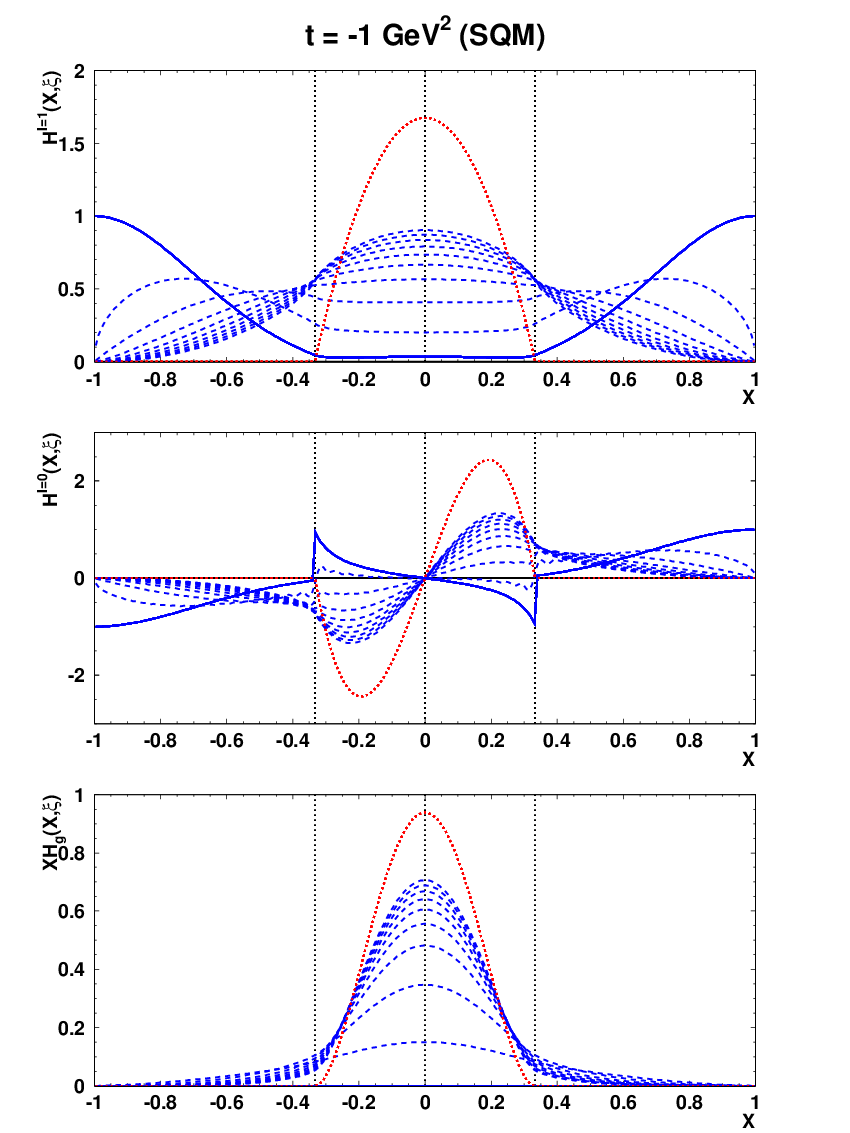
The results of the LO evolution from the SQM initial condition at the scale $Q_{0}$ up to $Q=4~{\rm GeV}$ and $\xi=1/3$ are shown in Figs. 13. In each set of the four plots, corresponding to a different value of $t$ , we show the quark non-singlet $H^{I=1}$ (top) and singlet (middle) $H^{I=0}$ distributions together with the gluon $H_{g}$ (bottom), conventionally multiplied by $X$ . We have chosen the sample value $\xi=1/3$ , since the results are qualitatively similar for other values of $\xi$ . The solid lines show the initial condition at the quark-model scale $Q_{0}$ of Eq. (70), the dashed lines show the result of the LO QCD evolution to the scale $Q=4~{\rm GeV}$ , and the dotted lines show the asymptotic forms at $Q\to\infty$ given in Eq. (83). As the value of $-t$ is increased, the magnitudes of the curves becomes lower, conforming to the sum rules (15,16). We note that the evolution smooths out the original distributions, in particular, the discontinuities at the end-points, $X=\pm 1$ , and at the ERBL-DGLAP matching points $X=\pm\xi$ disappear for the isosinglet GPD.

The results for the NJL model are very similar to the case of SQM. In Fig. 14 we show them for $t=-1~{\rm GeV}^{2}$ and $\xi=1/3$ . This similarity between the models is a sheer reflection of the numerical similarity in the initial condition, cf. Fig. 13 for $t=-1~{\rm GeV}^{2}$ and Fig. 14.

In Fig. 15 it is shown how slow the evolution is in reaching the asymptotic forms of the GPDF’s. The evolution is fastest at low values of $Q$ , where the coupling constant is large, and it immediately pulls down the end-point values to zero. Then, the strength gradually drifts from the DGLAP regions to the ERBL region. Yet, the approach to the asymptotic form is very slow, with the tails in the DGLAP region present. The highest $Q^{2}$ displayed in the figure is $10^{8}$ GeV² and the asymptotic form is reached at “cosmologically” large values of $Q$ , which are never achieved experimentally. Thus, the only way to approach the asymptotics would be to start from initial conditions which are already close to it. We also observe that a larger $-t$ more strength of the quark GPDs resides in the DGLAP region. This feature reflects the shape of the initial condition, which inhibits the strength in the ERBL region. Evolution up to $Q=2$ GeV retains this behavior, which gradually disappears as $Q\to\infty$ where all the strength settles in the ERBL region.

We note that the desired vanishing of the GPD’s at the end-points $X=\pm 1$ is achieved due to the QCD evolution, similarly to the results presented in Sec. V.5. Also, evolution leads to continuity at the DGLAP-ERBL boundary, $X=\pm\xi$ . These features are achieved at scales $Q$ infinitesimally above $Q_{0}$ .

VII Conclusions

We summarize our main points. In the present paper we have dealt with the determination of the leading twist GPD’s of the pion in field theoretic chiral quark models. We have done so with the help of an efficient method using the $\alpha$ -representation of the quark propagators and an extensive use of double distributions. Our calculation incorporates the necessary $D$ -terms required by polynomiality and dimensional analysis. In the chiral limit, we have been able to determine explicit analytic formulas for the pion GPD’s. All a priori properties which ought to be satisfied on general principles, namely polynomiality, positivity, proper support, soft-pion theorems, sum rules and normalization are indeed fulfilled explicitly by our model calculation. Although one might superficially think that these properties should be trivially satisfied, the fact that one deals with regularization or momentum dependence makes the fulfillment of those properties less obvious, and in fact many calculations violate some property. A key ingredient in our approach has been a scrupulous treatment of regularization in conjunction with electromagnetic and chiral Ward-Takahashi identities. Our results for the pionic GPD’s in the NJL model agree with Ref. Theussl et al. 2004.

In the two chiral quark models considered, NJL and SQM, we have found results looking alike since the models are mainly fixed by the pion charge form factor which in both cases looks very similar. In addition, we have determined the pion gravitational form factor entering the momentum-conservation sum rule. The outcoming GPD’s are not $t$ -factorizable, an assumption which is being extensively used in phenomenological approaches, not based on consistent dynamical calculations.

However, with all those desirable properties fulfilled, one must undertake the ERBL-DGLAP QCD evolution in order to relate the model results to experimental high-energy data where higher-twist contributions to the GPD’s can be disregarded. Likewise, a comparison to lattice results of the twist-2 GPD’s requires specification of a running scale. This aspect of the calculation is most frequently ignored in dynamical model calculations, and particularly in chiral quark models. A practical comparison to either experiment or lattice can be be achieved by matching the momentum fraction of the QCD evolved quark model to the experimental or lattice-extracted result. In practice, the LO perturbative evolution is used with the result that the low-energy quark-model scale is very low. Nevertheless, once this is fixed the GPD’s are uniquely determined. We have confronted our predictions with all available information extracted either from experiment or lattice both transverse or Euclidean. The experimental data include the Fermilab E615 and E791 measurements of PDF and PDA of the pion, respectively, and CLEO measuraments on the pion transition form factor. The reasonable overall agreement to all these data corresponding to quite different kinematical situations should be stressed. This fact provides some confidence on our predictions of the non-singlet leading twist GPD’s. This also applies to the pion-photon Transition Distribution Amplitude, determined recently in quark models Broniowski and Arriola 2007.

Acknowledgements.

We warmly thank Sasha Bakulev and Simon Dalley for providing us with the experimental and transverse lattice data, respectively.

Appendix A The $\alpha$ -representation evaluation of the two- and three-point functions

In studies based on quark models the simplest way to obtain the GPD’s and the double distributions is through the use of the $\alpha$ -representation for the scalar propagators. The advantage of this representation over other popular Feynman parameterizations of one-loop functions relies in the fact that the $\delta(k\cdot n-x)$ function constraining the loop integration is also naturally written in terms of an integral of an exponential. This allows for maintaining the explicit Lorentz covariance throughout the calculation. In our scheme one does not have to start with the somewhat cumbersome moments in $k\cdot n$ , and then “invert” the result, as is frequently done. The method used in this paper leads to well-defined and very simple algebra and reproduces the double distributions in chiral quark models from the literature. Also, in our approach the otherwise subtle effect of the emergence of the $D$ -terms follows in a clear way just from the Feynman diagrams.

Below we derive basic integrals appearing later on in the evaluation of the GPD’s. Calculations of this Appendix are made in the Euclidean space. We denote the Euclidean scalar propagators of particles of mass $\omega$ as

\displaystyle S_{k}=\frac{1}{D_{k}}=\frac{1}{k^{2}+\omega^{2}}=\int_{0}^{\infty}d\alpha e^{-\alpha(k^{2}+\omega^{2})},

(85)

where the RHS displays the $\alpha$ -representation.

A.1 Two-point functions

Let us first consider the function $I(x,l\cdot n,0,l^{2})$ corresponding to the definition (32) with the choice $l^{\prime}=0$ . This two-point function with the constrained $k\cdot n$ integration can be written as

$\displaystyle I(x,\kappa,0,l^{2})$	$\displaystyle=$	$\displaystyle\frac{4N_{c}w^{2}}{f^{2}}\int\frac{d^{4}k}{(2\pi)^{4}}\delta(k\cdot n-x)S_{k}S_{k-l}=\frac{4N_{c}w^{2}}{f^{2}}\int\frac{d^{4}k}{(2\pi)^{4}}\int\frac{d\lambda}{2\pi}e^{i\lambda(k\cdot n-x)}\!\int_{0}^{\infty}\!\!\!\!\!da\int_{0}^{\infty}\!\!\!\!\!\!dbe^{-a(k^{2}+\omega^{2})-b((k-l)^{2}+\omega^{2})}$	(86)
	$\displaystyle=$	$\displaystyle\frac{4N_{c}w^{2}}{f^{2}}\int\frac{d^{4}k^{\prime}}{(2\pi)^{4}}\int_{0}^{\infty}\!\!\!\!\!da\int_{0}^{\infty}\!\!\!\!\!db\int\frac{d\lambda^{\prime}}{2\pi}(a+b)e^{-(a+b)(k^{\prime 2}+\omega^{2})-\frac{ab}{a+b}l^{2}+i\lambda^{\prime}(b\kappa-(a+b)x)}$
	$\displaystyle=$	$\displaystyle\frac{4N_{c}w^{2}}{f^{2}}\int\frac{d^{4}k^{\prime}}{(2\pi)^{4}}\int_{0}^{\infty}\!\!\!\!\!da\int_{0}^{\infty}\!\!\!\!\!db\delta[b\kappa-(a+b)x](a+b)e^{-(a+b)(k^{\prime 2}+\omega^{2})-\frac{ab}{a+b}l^{2}},$

where for brevity $\kappa=n\cdot l$ , the shifted integration momentum is $k^{\prime}=k+\frac{b}{a+b}l+\frac{i}{2}\lambda^{\prime}n$ , and $\lambda^{\prime}=\lambda/(a+b)$ . The $\delta[b\kappa-(a+b)x]$ function gives the constraint

\displaystyle x=\frac{b\kappa}{a+b}.

(87)

Since the integration variables are positive, $a,b\geq 0$ , it follows immediately that $x\in[0,\kappa]$ for $\kappa\geq 0$ and $x\in[-\kappa,0)$ for $\kappa<0$ . This provides the proper support for $I(x,\kappa,0,l^{2})$ , which can be written generally as $\theta[x(\kappa-x)]$ .

One can decompose the $k^{\prime}$ integration into two parts,

\displaystyle dk^{\prime 0}dk^{\prime 3}=\pi dK^{2},\;\;\;dk^{\prime 1}dk^{\prime 2}=\pi du,

(88)

with $K^{2}=(k^{\prime 0})^{2}+(k^{\prime 3})^{2}$ and the “transverse” momentum $u=(k^{\prime 1})^{2}+(k^{\prime 2})^{2}$ . Then

	$\displaystyle I(x,\kappa,0,l^{2})$	$\displaystyle=$	$\displaystyle\frac{N_{c}\omega^{2}\theta[x(\kappa-x)]}{4\pi^{2}f^{2}}\int_{0}^{\infty}\!\!\!\!du\int_{0}^{\infty}\!\!\!\!da\int_{0}^{\infty}\!\!\!\!db\,\delta[b\kappa-(a+b)x]e^{-(a+b)(u+\omega^{2})-\frac{ab}{a+b}l^{2}}$		(89)
		$\displaystyle=$	$\displaystyle\frac{N_{c}\omega^{2}\theta[x(\kappa-x)]}{4\pi^{2}f^{2}\|\kappa\|}\int_{0}^{\infty}\!\!\!\!\!du\int_{0}^{\infty}db^{\prime}e^{-b^{\prime}\left[u+w^{2}+\frac{x}{\kappa}\left(1-\frac{x}{\kappa}\right)\right]}=\frac{N_{c}\omega^{2}\theta[x(\kappa-x)]}{4\pi^{2}f^{2}\|\kappa\|}\int_{0}^{\infty}\!\!\!\!du\frac{1}{u+w^{2}+\frac{x}{\kappa}\left(1-\frac{x}{\kappa}\right)l^{2}},$		(89)

where $b^{\prime}=b\kappa/x$ . The integral over $u$ is logarithmically divergent, hence needs regularization, as expected.

The general function $I(x,\kappa,\kappa^{\prime},(l-l^{\prime})^{2})$ , where $\kappa^{\prime}=n\cdot l^{\prime}$ , involves no extra work, as it can be obtained from the $l^{\prime}=0$ case with the replacement

\displaystyle k\to k-l^{\prime},\;\;l\to l-l^{\prime},\;\;x\to x-\kappa^{\prime},\;\;\kappa\to\kappa-\kappa^{\prime}.

(90)

This yields

	$\displaystyle I(x,\kappa,\kappa^{\prime},(l-l^{\prime})^{2})=\frac{N_{c}\omega^{2}\theta[(x-\kappa^{\prime})(\kappa-x)]}{4\pi^{2}f^{2}\|\kappa-\kappa^{\prime}\|}\times$
	$\displaystyle\;\;\;\;\int_{0}^{\infty}\!\!\!\!du\frac{1}{u+w^{2}+\frac{x-\kappa^{\prime}}{\kappa-\kappa^{\prime}}\left(1-\frac{x-\kappa^{\prime}}{\kappa-\kappa^{\prime}}\right)(l-l^{\prime})^{2}}.$		(91)

An important consequence of Lorentz invariance is polynomiality Ji 1998. We verify it by introducing the variable $\nu=(x-\kappa^{\prime})/(\kappa-\kappa^{\prime})$ , when $I(x,\kappa,\kappa^{\prime},(l-l^{\prime})^{2})$ becomes a function of $\nu$ devided by $|\kappa-\kappa^{\prime}|$ . We obtain (assuming for definiteness $\kappa>\kappa^{\prime}$ )

	$\displaystyle\int_{-1}^{1}dxI(x,\kappa,\kappa^{\prime},(l-l^{\prime})^{2})x^{n}=$
	$\displaystyle\;\;\;\;\;\int_{0}^{1}d\nu f(\nu)[\kappa^{\prime}+\nu(\kappa-\kappa^{\prime})]^{n},$		(92)

which results in a polynomial in $\kappa$ and $\kappa^{\prime}$ of the order at most $n$ . The first few moments have the explicit form

	$\displaystyle\int_{-1}^{1}dxI(x,\kappa,\kappa^{\prime},\tau)=\frac{N_{c}\omega^{2}\tau}{4\pi^{2}f^{2}}\int_{0}^{\infty}du\frac{2\log\left(\frac{\sqrt{4A+1}-1}{\sqrt{4A+1}+1}\right)}{\sqrt{4A+1}},$
	$\displaystyle\int_{-1}^{1}dxI(x,\kappa,\kappa^{\prime},\tau)\,x=\frac{N_{c}\omega^{2}\tau}{4\pi^{2}f^{2}}\int_{0}^{\infty}du\frac{(\kappa+\kappa^{\prime})\log\left(\frac{\sqrt{4A+1}-1}{\sqrt{4A+1}+1}\right)}{\sqrt{4A+1}},$
	$\displaystyle\int_{-1}^{1}dxI(x,\kappa,\kappa^{\prime},\tau)\,x^{2}=\frac{N_{c}\omega^{2}\tau}{4\pi^{2}f^{2}}\int_{0}^{\infty}du\times$
	$\displaystyle\;\;\;\frac{(4A+1)\left(\kappa-\kappa^{\prime}\right)^{2}-\sqrt{4A+1}\log\left(\frac{\sqrt{4A+1}+1}{\sqrt{4A+1}-1}\right)\left((2A+1)\kappa^{2}-4A\kappa^{\prime}\kappa+(2A+1)\left(\kappa^{\prime}\right)^{2}\right)}{4A+1},$		(93)

where $A=(u+\omega^{2})/\tau$ and $\tau=(l-l^{\prime})^{2}$ .

In the literature the $D$ -term is by definition the two-point function in the $t$ -channel Polyakov and Weiss 1999a. It originates from the diagram with the contact pion-quark term as well as from the reduced three-point diagram, where by “reduction” one means the replacement of $k^{2}$ and $k\cdot l$ pieces appearing in the numerator from the trace factor, in terms of the inverse scalar propagators. The two-point functions in the $s$ -channel (resulting from the reduction of the three-point function) are traditionally treated as singular parts of the double distributions.

A.2 Three-point functions

For the three-point functions we proceed analogously, now with three scalar propagators. We need to take into account the kinematics of the direct and crossed diagrams of Fig. 1. We first analyze in detail the the three-point function resulting from the direct diagram (a), since the case of the crossed diagram is obtained via a simple kinematic transformation. We have

	$\displaystyle J(x,q\cdot n,p\cdot n,q^{2},p^{2},p\cdot q)$	$\displaystyle=$	$\displaystyle\frac{4N_{c}\omega^{2}}{f^{2}}\!\int\frac{d^{4}k}{(2\pi)^{4}}\delta(k\cdot n-x)S_{k}S_{k+q}S_{bk-p}$		(94)
		$\displaystyle=$	$\displaystyle{4N_{c}\omega^{2}}{f^{2}}\!\int\frac{d^{4}k}{(2\pi)^{4}}\int\frac{d\lambda}{2\pi}e^{i\lambda(k\cdot n-x)}\int_{0}^{\infty}\!\!\!\!\!da\int_{0}^{\infty}\!\!\!\!\!db\int_{0}^{\infty}\!\!\!\!\!dce^{-a(k^{2}+\omega^{2})-b((k+q)^{2}+\omega^{2})-c((k-p)^{2}+\omega^{2})}.$		(94)

Shifting the integration variable, $k^{\prime}=k+(\beta q-\gamma p-i\lambda n/2)/(\alpha+\beta+\gamma)$ , and carrying over the $d^{4}k^{\prime}$ integration yields

\displaystyle\!\!\!\!J

\displaystyle=

\displaystyle\frac{N_{c}\omega^{2}}{4\pi^{2}f^{2}}\int_{0}^{\infty}\!\!\!\!\!da\int_{0}^{\infty}\!\!\!\!\!db\int_{0}^{\infty}\!\!\!\!\!dc\,\frac{1}{(a+b+c)^{2}}\delta\left(x-\frac{cp\cdot n-bq\cdot n}{a+b+c}\right)e^{-(a+b+c)\omega^{2}-\frac{b(a+c)}{a+b+c}q^{2}-\frac{c(a+b)}{a+b+c}p^{2}-\frac{2bc}{a+b+c}p\cdot q}.

(95)

Next, we change the variables into

\displaystyle s=a+b+c,\;\;y=\frac{b}{s},\;\;z=\frac{c}{s}.

(96)

Note that since $a,b,c\geq 0$ , we get $0\leq y,z\leq 1$ and also $y+z\leq 1$ . The substitution and integration over $s$ yields

	$\displaystyle J$	$\displaystyle=$	$\displaystyle\frac{N_{c}\omega^{2}}{4\pi^{2}f^{2}}\times$		(97)
			$\displaystyle\int_{0}^{1}\!\!dy\int_{0}^{1}\!\!dz\frac{\theta(1-y-z)\delta\left(x-zp\cdot n+yq\cdot n\right)}{\omega^{2}+y(1-y)q^{2}+z(1-z)p^{2}+2yzp\cdot q}.$		(97)

We note that polynomiality is obvious from this form, as multiplication by the power $x^{n}$ is equivalent to the multiplication by the factor $(zp\cdot n-yq\cdot n)^{n}$ . In the chiral limit of $m_{\pi}=0$ the first few moments are relatively simple:

	$\displaystyle\int_{0}^{1}\!\!\!\!dx\,J=\frac{N_{c}\omega^{2}}{4\pi^{2}f^{2}t}2\left[\arctan\left(\frac{\sqrt{t}}{\sqrt{4w^{2}-t}}\right)\right]^{2},$		(98)
	$\displaystyle\int_{0}^{1}\!\!\!\!dx\,J\,x=\frac{N_{c}\omega^{2}}{4\pi^{2}f^{2}t^{3/2}}2\left(\sqrt{t}\left[\arctan\left(\frac{\sqrt{t}}{\sqrt{4w^{2}-t}}\right)\right]^{2}-\sqrt{4w^{2}-t}(\zeta-2)\arctan\left(\frac{\sqrt{t}}{\sqrt{4w^{2}-t}}\right)+\sqrt{t}(\zeta-2)\right),$
	$\displaystyle\int_{0}^{1}\!\!\!\!dx\,J\,x^{2}=\frac{N_{c}\omega^{2}}{4\pi^{2}f^{2}t^{2}}\left[t(\zeta(\zeta+3)-7)+\right.$
	$\displaystyle\;\;\;\;\;\left.\arctan\left(\frac{\sqrt{t}}{\sqrt{4w^{2}-t}}\right)\left(\sqrt{t}\sqrt{4w^{2}-t}(6-\zeta(\zeta+2))+2\left(t-2w^{2}(\zeta-1)\right)\arctan\left(\frac{\sqrt{t}}{\sqrt{4w^{2}-t}}\right)\right)\right].$

We can rewrite Eq. (97) as

	$\displaystyle{\cal F}(z,y)$	$\displaystyle=$	$\displaystyle\frac{N_{c}\omega^{2}}{4\pi^{2}f^{2}}\frac{\theta(1-y-z)}{\omega^{2}-y(1-y-z)t-z(1-z)m_{\pi}^{2}},$
	$\displaystyle J(x)$	$\displaystyle=$	$\displaystyle\int_{0}^{1}\!\!dy\int_{0}^{1}\!\!dz\delta\left(x-z-y\zeta\right){\cal F}(z,y),$

where we have used the kinematics (7). The curly ${\cal F}$ denotes the double distribution.

Let us denote

\displaystyle\!\!\!\!\!\!\!\!{\cal D}={\omega^{2}-y(1-y-z)t-z(1-z)m_{\pi}^{2}}.

(100)

For the GPD of the pion, due to the crossing symmetry, one may assume $0\leq\zeta\leq 1$ . Next, we perform the $z$ integration, which sets

\displaystyle z=x-y\zeta.

(101)

The distributions in Eq. (97) give the following limits for the $y$ integration:

	$\displaystyle\!\!\!\!\!\!\!J=\frac{N_{c}\omega^{2}}{4\pi^{2}f^{2}}\left(\theta[x(\zeta-x)]\!\!\int_{0}^{\frac{x}{\zeta}}\!\!+\theta[(x-\zeta)(1-x)]\!\!\int_{0}^{\frac{1-x}{1-\zeta}}\right)\frac{dy}{\cal D},$
			(102)

with the first term having the support $x\in[0,\zeta]$ , and the second $x\in[\zeta,1]$ . The function $F(x)$ is continuous, but the derivative $dF(x)/dx$ is discontinuous at the points $x=0,\zeta,1$ . The double distribution is München-symmetric Mankiewicz et al. 1998, i.e. ${\cal F}(z,y)={\cal F}(z,1-y-z)$ . This feature is related to the crossing symmetry, holding for identical particles.

The result for the crossed diagram (see Fig. 1 is obtained from the above result for the direct diagram with the replacement $p\to-p-q$ . Replacing correspondingly $x\to\zeta-x$ and performing the München transformation Mankiewicz et al. 1998

\displaystyle z\to z,\;\;\;y\to 1-y-z,

(103)

we find that ${\cal D}$ is invariant under this joint transformation. The function $\delta(x-z-y\zeta)$ is also invariant under these combined two trasformations. Finally, the support is invariant, since

	$\displaystyle\theta(1-y-z)\theta[y(1-y)]\theta[z(1-z)]\to$
	$\displaystyle\;\;\;\;\theta(y)\theta[(1-y-z)(y+z)]\theta[z(1-z)]$
	$\displaystyle\;\;\;\;=\theta(1-y-z)\theta[y(1-y]\theta[z(1-z)],$		(104)

where the equality in the above formula is an algebraic identity. Therefore the crossed diagram is related to the direct diagram as follows:

\displaystyle J^{\rm crossed}(x,\zeta)=J^{\rm direct}(\zeta-x,\zeta).

(105)

The support of the crossed diagram reflects the support of the direct diagram, i.e., $x\in[-1+\zeta,\zeta]$ .

Appendix B The two- and three-point functions in the Spectral Quark Model

According to the general rule, in SQM one append the formulas with the spectral integration $\int_{C}d\omega\omega^{2}\rho(\omega)$ . The results below are for the meson-dominance model.

B.1 The two-point function

We assume $\kappa^{\prime}\leq\kappa$ . The spectral integration yields

	$\displaystyle I_{\rm SQM}(x,\kappa,\kappa^{\prime},l^{2})=\int_{C}d\omega\omega^{2}\rho(\omega)I(x,\kappa,\kappa^{\prime},l^{2})$
	$\displaystyle=\frac{\theta[(x-\kappa^{\prime})(\kappa-x)]}{(\kappa-\kappa^{\prime})\left[1+4\frac{x-\kappa^{\prime}}{\kappa-\kappa^{\prime}}\left(1-\frac{x-\kappa^{\prime}}{\kappa-\kappa^{\prime}}\right)\frac{l^{2}}{M_{V}^{2}}\right]^{3/2}},$		(106)

where we have used the relation

\displaystyle M_{V}^{2}=24\pi^{2}f^{2}/N_{c}.

(107)

The integration over $x$ yields the form factor

\displaystyle\int dxI_{\rm SQM}(x,\kappa,\kappa^{\prime},l^{2})=\frac{M_{V}^{2}}{M_{V}^{2}+l^{2}}.

(108)

In agreement with polynomiality, this form factor is independent of the value of $\kappa$ or $\kappa^{\prime}$ . Note that the vector-meson dominance is readily obtained. Similarly,

\displaystyle\int dxI_{\rm SQM}(x,\kappa,\kappa^{\prime},l^{2})\,x=\frac{M_{V}^{2}}{M_{V}^{2}+l^{2}}\frac{\kappa+\kappa^{\prime}}{2}.

(109)

B.2 The three-point function

For simplicity in this Appendix we work in the chiral limit. In this case the double distribution becomes

\displaystyle{\cal F}_{\omega}(z,y;t)

\displaystyle=

\displaystyle\frac{N_{c}\omega^{2}}{4\pi^{2}f^{2}}\frac{\theta(1-y-z)}{\omega^{2}-y(1-y-z)t},

(110)

and the subsequent spectral integration yields (again we only multiply by $\omega^{2}$ and leave out other factors)

	$\displaystyle{\cal F}_{\rm SQM}(z,y;t)$	$\displaystyle=$	$\displaystyle\int_{C}d\omega\rho(\omega){\cal F}_{\omega}(z,y;t)$		(111)
		$\displaystyle=$	$\displaystyle\frac{N_{c}}{4\pi^{2}f^{2}}\frac{\theta(1-y-z)}{\left(1-\frac{4y(1-y-z)t}{M_{V}^{2}}\right)^{5/2}}.$		(111)

Let us introduce the short-hand notation

	$\displaystyle\chi_{2}$	$\displaystyle=$	$\displaystyle\frac{2(x-1)\left[3(\zeta-1)M_{V}^{2}+t(x-1)^{2}\right]}{\left[(\zeta-1)M_{V}^{2}+t(x-1)^{2}\right]^{2}},$
	$\displaystyle\chi_{1}$	$\displaystyle=$	$\displaystyle\frac{(x(\zeta-2)+\zeta)\left(3M_{V}^{2}(\zeta-1)\zeta^{2}+t\left(\left(\zeta^{2}+8\zeta-8\right)x^{2}+2(4-5\zeta)\zeta x+\zeta^{2}\right)\right)}{\left((\zeta-1)M_{V}^{2}+t(x-1)^{2}\right)^{2}\left({\zeta^{2}+\frac{4tx(x-\zeta)}{M_{V}^{2}}}\right)^{3/2}}+\frac{1}{2}\chi_{2}.$		(112)

Then, for the case $\zeta\geq 0$ ,

\displaystyle J_{\rm SQM}(x,\zeta;t)

\displaystyle=

\displaystyle\left(\theta[x(\zeta-x)]\chi_{1}+\theta[(1-x)(x-\zeta)]\chi_{2}\right).

The function satisties $J_{\rm SQM}(0,\zeta;t)=J_{\rm SQM}(1,\zeta;t)=0$ . The value at the matching point $x=\zeta$ is

\displaystyle J_{\rm SQM}(\zeta,\zeta;t)=\frac{2\left(3M_{V}^{2}+t(\zeta-1)\right)}{\left(M_{V}^{2}+t(\zeta-1)\right)^{2}}.

(114)

The integration over $x$ produces a $\zeta$ -independent (as required by polynomiality) form factor,

\displaystyle\int_{0}^{1}\!\!dxJ_{\rm SQM}(x,\zeta;t)=\frac{2}{M_{V}^{2}-t}-\frac{\log\left(1-\frac{t}{M_{V}^{2}}\right)}{t}.

(115)

Similarly,

\displaystyle\int_{0}^{1}\!\!dxJ_{\rm SQM}(x,\zeta;t)\,x=\frac{\zeta}{M_{V}^{2}-t}-\frac{\log\left(1-\frac{t}{M_{V}^{2}}\right)}{t}.

(116)

For the special case of $t=0$ Eq. () reduces to the very simple expression

	$\displaystyle J_{\rm SQM}(x,\zeta;0)$	$\displaystyle=$	$\displaystyle\frac{6}{M_{V}^{2}}\left(\theta[x(\zeta-x)]\frac{x}{\zeta}\right.$
		$\displaystyle+$	$\displaystyle\left.\theta[(1-x)(x-\zeta)]\frac{x-1}{\zeta-1}\right),$

which is a triangle of area $3/M_{V}^{2}=N_{c}/(8\pi^{2}f^{2})$ .

For the case $\zeta=0$ we have

\displaystyle J_{\rm SQM}(x,0;t)

\displaystyle=

\displaystyle\frac{\left(3M_{V}^{2}-t(1-x)^{2}\right)(1-x)}{\left(M_{V}^{2}-t(1-x)^{2}\right)^{2}}.

(118)

Appendix C The two- and three-point functions in the NJL model

Operationally, the calculation in the NJL model with the regularization (53) amounts to taking the generic expressions (91) and (102), replacing $\omega^{2}\to M^{2}+\Lambda^{2}$ in the denominators, carry out the integrations, and finally applying (53). We work in the chiral limit.

C.1 The two-point function

Through the use of Eq. (54) we arrive immediately at the formula (for $\kappa\geq\kappa^{\prime}$ )

\displaystyle I_{\rm NJL}(x,\kappa,\kappa^{\prime},0)=\frac{\theta[(x-\kappa^{\prime})(\kappa-x)]}{\kappa-\kappa^{\prime}}.

(119)

C.2 The three-point function

We find

	$\displaystyle J_{\rm NJL}(x,\zeta;m_{\pi}=0;\Lambda)=-\frac{N_{c}M^{2}}{8\pi^{2}f^{2}}\left[\frac{2\log\left(\frac{\sqrt{-t}(x-1)+\sqrt{-t(x-1)^{2}-4(\zeta-1)\left(M^{2}+\Lambda^{2}\right)}}{\sqrt{-t(x-1)^{2}-4(\zeta-1)\left(M^{2}+\lambda^{2}\right)}-\sqrt{-t}(x-1)}\right)\theta((1-x)(x-\zeta))}{\sqrt{-t}\sqrt{-t(x-1)^{2}-4(\zeta-1)\left(M^{2}+\lambda^{2}\right)}}+\right.$		(120)
	$\displaystyle\left.\frac{\left(\log\left(\frac{\sqrt{-t}(x-1)+\sqrt{-t(x-1)^{2}-4(\zeta-1)\left(M^{2}+\lambda^{2}\right)}}{\sqrt{-t(x-1)^{2}-4(\zeta-1)\left(M^{2}+\lambda^{2}\right)}-\sqrt{-t}(x-1)}\right)+\log\left(\frac{\sqrt{-t(x-1)^{2}-4(\zeta-1)\left(M^{2}+\lambda^{2}\right)}\zeta+\sqrt{-t}(x(\zeta-2)+\zeta)}{\zeta\sqrt{-t(x-1)^{2}-4(\zeta-1)\left(M^{2}+\lambda^{2}\right)}-\sqrt{-t}(x(\zeta-2)+\zeta)}\right)\right)\theta(x(\zeta-x))}{\sqrt{-t}\sqrt{-t(x-1)^{2}-4(\zeta-1)\left(M^{2}+\lambda^{2}\right)}}\right],$

and

\displaystyle J_{\rm NJL}(x,\zeta;m_{\pi}=0)=\left.J_{\rm NJL}(x,\zeta;m_{\pi}=0;\Lambda)\right|_{\rm reg}.

(121)

Polynomiality follows from the fact that the expressions are derived from the double distributions () and the distributive nature of the regularization prescription (53). By distributive we mean that it is a sum over quark masses or the integral over $\omega$ of the formal expressions for $I$ and $J$ .

Appendix D The gravitational form factors

The gravitational form factors of the pion Donoghue and Leutwyler 1991 are defined through the matrix element of the energy-momentum tensor,

	$\displaystyle\!\!\!\!\!\!\langle\pi^{b}(p+q)\mid\theta^{\mu\nu}(0)\mid\pi^{a}(p)\rangle=$		(122)
	$\displaystyle\!\!\!\!\!\!\!\frac{\delta^{ab}}{2}\left(g^{\mu\nu}q^{2}-(q^{\mu}q^{\nu})\theta_{1}(q^{2})+(2p+q)^{\mu}(2p+q)^{\nu}\theta_{2}(q^{2})\right).$

They satisfy the low energy theorem $\theta_{1}(0)-\theta_{2}(0)={\cal O}(m_{\pi}^{2})$ Donoghue and Leutwyler 1991. The leading- $N_{c}$ quark-model evaluation amounts to computing the diagrams of Figs. 1 and 2 with the pion gravitational vertex

	$\displaystyle\theta^{\mu\nu}(k+q,k)=\frac{1}{4}\left((2k+q)^{\mu}\gamma^{\nu}+(2k+q)^{\nu}\gamma^{\mu}\right)$
	$\displaystyle-\frac{1}{2}g^{\mu\nu}\left(2\hbox to0.0pt{\hbox to5.52084pt{\hfil/\hfil}\hss}k+\hbox to0.0pt{\hbox to5.00002pt{\hfil$q$\hfil}\hss}/-\omega\right).$		(123)

The results of the calculation in SQM is Eq. (38). Equation (16) follows from considering the matrix element of $n_{\mu}\theta^{\mu\nu}n_{\nu}$ . Then

	$\displaystyle\langle\pi^{b}(p+q)\mid n_{\mu}\theta^{\mu\nu}(0)n_{\nu}\mid\pi^{a}(p)\rangle=$		(124)
	$\displaystyle\delta^{ab}\frac{1}{2}\left[\zeta^{2}\theta_{1}(q^{2})+(2-\zeta)^{2}\theta_{2}(q^{2})\right].$

The vertex becomes

\displaystyle n_{\mu}\theta^{\mu\nu}(k+q,k)n_{\nu}=(x-\zeta/2)\gamma\cdot n.

(125)

We notice it is the same vertex as in the evaluation of the GPD’s multiplied by $(x-\zeta/2)$ . Upon passing to the symmetric notation Eq. 16 follows.

Appendix E End-point analysis for the PDA

Here we derive the formulas used in the main text of Sect. V.5 for the PDA and correct a mistake in expressions of our previous work Ruiz Arriola and Broniowski 2002; Ruiz Arriola 2002. Right at the end-points, $x=0,1$ , the series (73) diverges since $C_{2k}^{3/2}(\pm 1)=\frac{1}{2}(2k+1)(2k+2)$ , meaning a non-uniform convergence as $x\to 0$ or $x\to 1$ as well as the large- $n$ dominance of the end-point behavior. In this limit we have Ruiz Arriola and Broniowski 2004

\displaystyle\left(\frac{\alpha(Q)}{\alpha(Q_{0})}\right)^{\gamma_{n}^{(0)}/(2\beta_{0})}\sim n^{-8r(Q_{0},Q)}e^{2(3-4\gamma)r(Q_{0},Q)}.

Only even- $n$ terms contribute in Eq. (73), hence we impose this condition for integer $n$ and then extend $n$ to real values. The summation in Eq. (73) is then replaced with an integral,

\displaystyle\phi(x,Q)

\displaystyle\sim

\displaystyle\frac{1}{2}8xe^{(3/4-\gamma)a}\int_{0}^{\infty}\!\!\!\!\!dn\,C_{n}^{\frac{3}{2}}(2x-1)n^{-a-1}\,,

where the factor of $1/2$ comes from the summation over even $n$ only, and

\displaystyle a=8r(Q_{0},Q).

(128)

The Gegenbauer polynomials $C_{n}^{\frac{3}{2}}(\xi)$ in the variable $\xi=2x-1$ satisfy the differential equation Abramowitz and Stegun 1964

\displaystyle(1-\xi^{2})y^{\prime\prime}(\xi)-4\xi y^{\prime}(\xi)+n(n+3)y(\xi)=0\,,

(129)

which upon the substitution

\displaystyle y(\xi)=\frac{u(\xi)}{1-\xi^{2}}\,,

(130)

transforms into a Schrödinger-like equation at zero energy,

\displaystyle u^{\prime\prime}(\xi)+\frac{n^{2}+3n+2}{1-\xi^{2}}u(\xi)=0\,.

(131)

Here the interval of interest, $-1\leq\xi\leq 1$ , corresponds to the classically allowed region and the potential is attractive. In the large- $n$ limit the solution oscillates rapidly and a semiclassical WKB approximation Galindo and Pascual 1991 might be used. Here in order to analyze the limit $x\to 0$ we consider the differential equation, Eq. (131), which in the limit $x\to 0$ and $n\gg 1$ transforms into a zero-energy Coulomb-like problem. Its solution can be generally written in terms of the Bessel functions,

\displaystyle C_{n}^{\frac{3}{2}}(2x-1)=\frac{c_{1}J_{1}(2n\sqrt{x})+c_{2}Y_{1}(2n\sqrt{x})}{\sqrt{x}}.

(132)

where actually $c_{2}=0$ , since the Gegenbauer polynomials are regular at the end-point $x=0$ . The undetermined constant $c_{1}$ may be obtained by matching the small argument expansion $J_{1}(z)=z/2+\dots$ to the value $C_{n}^{3/2}(1)\sim\frac{n^{2}}{2}$ , yielding for $n\gg 1$ and $x\to 0$ the formula

\displaystyle C_{n}^{\frac{3}{2}}(2x-1)\sim\frac{n}{2\sqrt{x}}J_{1}(2n\sqrt{x})\,.

(133)

As we see in the low- $x$ and large- $n$ limit there is a scaling behavior of the Gegenbauer polynomials,

\displaystyle C_{n}^{\frac{3}{2}}(x)\sim nF(n\sqrt{x})/\sqrt{x}\,.

(134)

From Eq. () it is now clear that this translates into the low- $x$ scaling behavior

\displaystyle\phi(x,Q)

\displaystyle\sim

\displaystyle x^{a/2}e^{(3/4-\gamma)a}\int_{0}^{\infty}\,dt\,F(t)t^{-a}\,.

(135)

Evaluation of the integral and collecting the factors yields Eq. (81).

References

Ji (1998) X.-D. Ji, J. Phys. G24, 1181 (1998), eprint hep-ph/9807358.
Radyushkin (2000) A. V. Radyushkin (2000), eprint hep-ph/0101225.
Goeke et al. (2001) K. Goeke, M. V. Polyakov, and M. Vanderhaeghen, Prog. Part. Nucl. Phys. 47, 401 (2001), eprint hep-ph/0106012.
Diehl (2003) M. Diehl, Phys. Rept. 388, 41 (2003), eprint hep-ph/0307382.
Ji (2004) X. Ji, Ann. Rev. Nucl. Part. Sci. 54, 413 (2004).
Belitsky and Radyushkin (2005) A. V. Belitsky and A. V. Radyushkin, Phys. Rept. 418, 1 (2005), eprint hep-ph/0504030.
Feldmann (2007) T. Feldmann, Eur. Phys. J. Special Topics 140, 135 (2007).
Boffi and Pasquini (2007) S. Boffi and B. Pasquini (2007), eprint arXiv:0711.2625 [hep-ph].
Belitsky et al. (2004) A. V. Belitsky, X.-d. Ji, and F. Yuan, Phys. Rev. D69, 074014 (2004), eprint hep-ph/0307383.
Collins et al. (1997) J. C. Collins, L. Frankfurt, and M. Strikman, Phys. Rev. D56, 2982 (1997), eprint hep-ph/9611433.
Szczepaniak et al. (2007) A. P. Szczepaniak, J. T. Londergan, and F. J. Llanes-Estrada (2007), eprint arXiv:0707.1239 [hep-ph].
Burkardt and Dalley (2002) M. Burkardt and S. Dalley, Prog. Part. Nucl. Phys. 48, 317 (2002), eprint hep-ph/0112007.
Hagler (2007) P. Hagler (2007), eprint arXiv:0711.0819 [hep-lat].
Ahmad et al. (2007) S. Ahmad, H. Honkanen, S. Liuti, and S. K. Taneja (2007), eprint arXiv:0708.0268 [hep-ph].
Diehl et al. (2005) M. Diehl, A. Manashov, and A. Schafer, Phys. Lett. B622, 69 (2005), eprint hep-ph/0505269.
Chen et al. (2007) J.-W. Chen, W. Detmold, and B. Smigielski, Phys. Rev. D75, 074003 (2007), eprint hep-lat/0612027.
Kivel and Polyakov (2007) N. Kivel and M. V. Polyakov (2007), eprint arXiv:0707.2208 [hep-ph].
Radyushkin (1999a) A. V. Radyushkin, Phys. Rev. D59, 014030 (1999a), eprint hep-ph/9805342.
Polyakov and Weiss (1999a) M. V. Polyakov and C. Weiss, Phys. Rev. D60, 114017 (1999a), eprint hep-ph/9902451.
Pire et al. (1999) B. Pire, J. Soffer, and O. Teryaev, Eur. Phys. J. C8, 103 (1999), eprint hep-ph/9804284.
Pobylitsa (2002) P. V. Pobylitsa, Phys. Rev. D65, 077504 (2002), eprint hep-ph/0112322.
Polyakov (1999) M. V. Polyakov, Nucl. Phys. B555, 231 (1999), eprint hep-ph/9809483.
Davidson and Ruiz Arriola (1995) R. M. Davidson and E. Ruiz Arriola, Phys. Lett. B348, 163 (1995).
Weigel et al. (1999) H. Weigel, E. Ruiz Arriola, and L. P. Gamberg, Nucl. Phys. B560, 383 (1999), eprint hep-ph/9905329.
Van Dyck et al. (2007) A. Van Dyck, T. Van Cauteren, and J. Ryckebusch (2007), eprint arXiv:0710.2271 [hep-ph].
Christov et al. (1996) C. V. Christov et al., Prog. Part. Nucl. Phys. 37, 91 (1996), eprint hep-ph/9604441.
Ruiz Arriola (2002) E. Ruiz Arriola, Acta Phys. Polon. B33, 4443 (2002), eprint hep-ph/0210007.
Ruiz Arriola (2001) E. Ruiz Arriola (2001), eprint hep-ph/0107087.
Ruiz Arriola and Broniowski (2003) E. Ruiz Arriola and W. Broniowski, Phys. Rev. D67, 074021 (2003), eprint hep-ph/0301202.
Davidson and Ruiz Arriola (2002) R. M. Davidson and E. Ruiz Arriola, Acta Phys. Polon. B33, 1791 (2002), eprint hep-ph/0110291.
Ruiz Arriola and Broniowski (2002) E. Ruiz Arriola and W. Broniowski, Phys. Rev. D66, 094016 (2002), eprint hep-ph/0207266.
Broniowski and Ruiz Arriola (2003) W. Broniowski and E. Ruiz Arriola, Phys. Lett. B574, 57 (2003), eprint hep-ph/0307198.
Pire and Szymanowski (2005a) B. Pire and L. Szymanowski, Phys. Rev. D71, 111501 (2005a), eprint hep-ph/0411387.
Pire and Szymanowski (2005b) B. Pire and L. Szymanowski, Phys. Lett. B622, 83 (2005b), eprint hep-ph/0504255.
Broniowski and Arriola (2007) W. Broniowski and E. R. Arriola, Phys. Lett. B649, 49 (2007), eprint hep-ph/0701243.
Anikin et al. (2000a) I. V. Anikin, A. E. Dorokhov, A. E. Maksimov, L. Tomio, and V. Vento, Nucl. Phys. A678, 175 (2000a).
Anikin et al. (2000b) I. V. Anikin, A. E. Dorokhov, A. E. Maksimov, and L. Tomio, Phys. Atom. Nucl. 63, 489 (2000b).
Dorokhov and Tomio (1998) A. E. Dorokhov and L. Tomio (1998), eprint hep-ph/9803329.
Dorokhov and Tomio (2000) A. E. Dorokhov and L. Tomio, Phys. Rev. D62, 014016 (2000).
Polyakov and Weiss (1999b) M. V. Polyakov and C. Weiss, Phys. Rev. D59, 091502 (1999b), eprint hep-ph/9806390.
Praszalowicz and Rostworowski (2003) M. Praszalowicz and A. Rostworowski, Acta Phys. Polon. B34, 2699 (2003), eprint hep-ph/0302269.
Bzdak and Praszalowicz (2003) A. Bzdak and M. Praszalowicz, Acta Phys. Polon. B34, 3401 (2003), eprint hep-ph/0305217.
Noguera and Vento (2006) S. Noguera and V. Vento, Eur. Phys. J. A28, 227 (2006), eprint hep-ph/0505102.
Bakulev et al. (2000) A. P. Bakulev, R. Ruskov, K. Goeke, and N. G. Stefanis, Phys. Rev. D62, 054018 (2000), eprint hep-ph/0004111.
Choi et al. (2001) H.-M. Choi, C.-R. Ji, and L. S. Kisslinger, Phys. Rev. D64, 093006 (2001), eprint hep-ph/0104117.
Choi et al. (2002) H.-M. Choi, C.-R. Ji, and L. S. Kisslinger, Phys. Rev. D66, 053011 (2002), eprint hep-ph/0204321.
Mukherjee et al. (2003) A. Mukherjee, I. V. Musatov, H. C. Pauli, and A. V. Radyushkin, Phys. Rev. D67, 073014 (2003), eprint hep-ph/0205315.
Tiburzi and Miller (2003a) B. C. Tiburzi and G. A. Miller, Phys. Rev. D67, 013010 (2003a), eprint hep-ph/0209178.
Tiburzi and Miller (2003b) B. C. Tiburzi and G. A. Miller, Phys. Rev. D67, 113004 (2003b), eprint hep-ph/0212238.
Radyushkin (1999b) A. V. Radyushkin, Phys. Lett. B449, 81 (1999b), eprint hep-ph/9810466.
Bissey et al. (2004) F. Bissey, J. R. Cudell, J. Cugnon, J. P. Lansberg, and P. Stassart, Phys. Lett. B587, 189 (2004), eprint hep-ph/0310184.
Theussl et al. (2004) L. Theussl, S. Noguera, and V. Vento, Eur. Phys. J. A20, 483 (2004), eprint nucl-th/0211036.
Conway et al. (1989) J. S. Conway et al., Phys. Rev. D39, 92 (1989).
Aitala et al. (2001) E. M. Aitala et al. (E791), Phys. Rev. Lett. 86, 4768 (2001), eprint hep-ex/0010043.
Donoghue and Leutwyler (1991) J. F. Donoghue and H. Leutwyler, Z. Phys. C52, 343 (1991).
Miller (2007) G. A. Miller, Phys. Rev. Lett. 99, 112001 (2007), eprint arXiv:0705.2409 [nucl-th].
Diehl et al. (1998) M. Diehl, T. Gousset, B. Pire, and O. Teryaev, Phys. Rev. Lett. 81, 1782 (1998), eprint hep-ph/9805380.
Ruiz Arriola (1991) E. Ruiz Arriola, Phys. Lett. B264, 178 (1991).
Arriola et al. (2007) E. R. Arriola, W. Broniowski, and B. Golli, Phys. Rev. D76, 014008 (2007), eprint hep-ph/0610289.
Ji (1995) X.-D. Ji, Phys. Rev. D52, 271 (1995), eprint hep-ph/9502213.
Altarelli and Parisi (1977) G. Altarelli and G. Parisi, Nucl. Phys. B126, 298 (1977).
Sutton et al. (1992) P. J. Sutton, A. D. Martin, R. G. Roberts, and W. J. Stirling, Phys. Rev. D45, 2349 (1992).
Gluck et al. (1999) M. Gluck, E. Reya, and I. Schienbein, Eur. Phys. J. C10, 313 (1999), eprint hep-ph/9903288.
Martinelli and Sachrajda (1988) G. Martinelli and C. T. Sachrajda, Nucl. Phys. B306, 865 (1988).
Best et al. (1997) C. Best et al., Phys. Rev. D56, 2743 (1997), eprint hep-lat/9703014.
Capitani et al. (2006) S. Capitani et al., Phys. Lett. B639, 520 (2006), eprint hep-lat/0511013.
Meyer and Negele (2007) H. B. Meyer and J. W. Negele (2007), eprint arXiv:0707.3225 [hep-lat].
Dalley (2001) S. Dalley, Phys. Rev. D64, 036006 (2001), eprint hep-ph/0101318.
Burkardt and Seal (2001) M. Burkardt and S. K. Seal, Phys. Rev. D64, 111501 (2001), eprint hep-ph/0105109.
Wijesooriya et al. (2005) K. Wijesooriya, P. E. Reimer, and R. J. Holt, Phys. Rev. C72, 065203 (2005), eprint nucl-ex/0509012.
Dalley and van de Sande (2003) S. Dalley and B. van de Sande, Phys. Rev. D67, 114507 (2003), eprint hep-ph/0212086.
Gluck et al. (1998) M. Gluck, E. Reya, and A. Vogt, Eur. Phys. J. C5, 461 (1998), eprint hep-ph/9806404.
Anikin et al. (2000c) I. V. Anikin, A. E. Dorokhov, and L. Tomio, Phys. Lett. B475, 361 (2000c), eprint hep-ph/9909368.
Dorokhov (2003) A. E. Dorokhov, JETP Lett. 77, 63 (2003), eprint hep-ph/0212156.
Bakulev et al. (2004) A. P. Bakulev, S. V. Mikhailov, and N. G. Stefanis, Phys. Lett. B578, 91 (2004), eprint hep-ph/0303039.
Bakulev et al. (2006) A. P. Bakulev, S. V. Mikhailov, and N. G. Stefanis, Phys. Rev. D73, 056002 (2006), eprint hep-ph/0512119.
Bakulev et al. (2007) A. P. Bakulev, S. V. Mikhailov, A. V. Pimikov, and N. G. Stefanis (2007), eprint arXiv:0710.2275 [hep-ph].
Lepage and Brodsky (1980) G. P. Lepage and S. J. Brodsky, Phys. Rev. D22, 2157 (1980).
Mueller (1995) D. Mueller, Phys. Rev. D51, 3855 (1995), eprint hep-ph/9411338.
Schmedding and Yakovlev (2000) A. Schmedding and O. I. Yakovlev, Phys. Rev. D62, 116002 (2000), eprint hep-ph/9905392.
Gronberg et al. (1998) J. Gronberg et al. (CLEO), Phys. Rev. D57, 33 (1998), eprint hep-ex/9707031.
Del Debbio et al. (2003) L. Del Debbio, M. Di Pierro, and A. Dougall, Nucl. Phys. Proc. Suppl. 119, 416 (2003), eprint hep-lat/0211037.
Braun et al. (2006) V. M. Braun et al., Phys. Rev. D74, 074501 (2006), eprint hep-lat/0606012.
Donnellan et al. (2007) M. A. Donnellan et al. (2007), eprint arXiv:0710.0869 [hep-lat].
Ruiz Arriola and Broniowski (2004) E. Ruiz Arriola and W. Broniowski, Phys. Rev. D70, 034012 (2004), eprint hep-ph/0404008.
Dalley (2003) S. Dalley, Phys. Lett. B570, 191 (2003), eprint hep-ph/0306121.
Dalley (2005) S. Dalley, Few Body Syst. 36, 69 (2005), eprint hep-ph/0409139.
Mueller et al. (1994) D. Mueller, D. Robaschik, B. Geyer, F. M. Dittes, and J. Horejsi, Fortschr. Phys. 42, 101 (1994), eprint hep-ph/9812448.
Ji (1997) X.-D. Ji, Phys. Rev. D55, 7114 (1997), eprint hep-ph/9609381.
Radyushkin (1997) A. V. Radyushkin, Phys. Rev. D56, 5524 (1997), eprint hep-ph/9704207.
Blumlein et al. (1997) J. Blumlein, B. Geyer, and D. Robaschik, Phys. Lett. B406, 161 (1997), eprint hep-ph/9705264.
Golec-Biernat and Martin (1999) K. J. Golec-Biernat and A. D. Martin, Phys. Rev. D59, 014029 (1999), eprint hep-ph/9807497.
Kivel and Mankiewicz (1999a) N. Kivel and L. Mankiewicz, Nucl. Phys. B557, 271 (1999a), eprint hep-ph/9903531.
Kivel and Mankiewicz (1999b) N. Kivel and L. Mankiewicz, Phys. Lett. B458, 338 (1999b), eprint hep-ph/9905342.
Mankiewicz et al. (1998) L. Mankiewicz, G. Piller, and T. Weigl, Eur. Phys. J. C5, 119 (1998), eprint hep-ph/9711227.
Abramowitz and Stegun (1964) M. Abramowitz and I. A. Stegun, Handbook of Mathematical Functions (Dover Publications, 1964).
Galindo and Pascual (1991) A. Galindo and P. Pascual, Quantum Mechanics (Springer, 1991).