Estimating the total infrared luminosity of galaxies up to from mid- and far-infrared observations
Abstract
Aims. We present the observed correlations between rest-frame 8, 24, 70 and 160 m monochromatic luminosities and measured total infrared luminosities of galaxies detected by Spitzer.
Methods. Our sample consists of 372 star-forming galaxies with individual detections and flux measurements at 8, 24, 70 and 160 m. We have spectroscopic redshifts for 93% of these sources, and accurate photometric redshifts for the remainder. We also used a stacking analysis to measure the IR fluxes of fainter sources at higher redshifts.
Results. We show that the monochromatic mid and far-infrared luminosities are strongly correlated with the total infrared luminosity and our stacking analysis confirms that these correlations also hold at higher redshifts. We provide relations between monochromatic luminosities and total infrared luminosities that should be reliable up to () for ULIRGs (LIRGs). In particular, we can predict with accuracies of 37% and 54% from the 8 and 24 m fluxes, while the best tracer is the 70 m flux. Combining bands leads to slightly more accurate estimates. For example, combining the 8 and 24 m luminosities predicts with an accuracy of 34%. Our results are generally compatible with previous studies, and the small changes are probably due to differences in the sample selection criteria. We can rule out strong evolution in dust properties with redshift up to . Finally, we show that infrared and sub-millimeter observations are complementary means of building complete samples of star-forming galaxies, with the former being more sensitive for and the latter at higher .
Key Words.
Infrared: galaxies – Galaxies: Starburst – Galaxies: fundamental parameters – Galaxies: Evolution1 Introduction
Bright infrared galaxies play an important role in understanding the evolution of galaxies because a large fraction of the energy from star formation is reprocessed by dust and only visible in the infrared. This emission is dominated by the luminous infrared galaxies (LIRGs, defined by ) at (Le Floc’h et al. 2005, e.g.) and by ultra-luminous infrared galaxies (ULIRGs, defined by ) at (Caputi et al. 2007, e.g.). The LIRGs and ULIRGs are massive star-forming galaxies (Swinbank et al. 2004; Caputi et al. 2006) but some of the emission may also come from embedded AGN (Alonso-Herrero et al. 2006, e.g.). For systems dominated by star formation, the total infrared luminosity emitted between a few m and 1 mm is a good tracer of the star formation rate (Kennicutt 1998). Thus estimating the infrared luminosity of galaxies is important for quantifying star formation activity.
Measuring the spectral energy distribution (SED) of infrared galaxies also probes physical properties such as their dust temperature, or grain size and composition. Models of nearby objects using IRAS, ISO and Spitzer have shown that the typical infrared galaxy SED peaks between 60 and 150m, depending on the dust temperature (Kennicutt et al. 2003, e.g. the Spitzer Nearby Galaxy Survey, ).
The far-infrared bands on Spitzer (the MIPS 70 and 160m bands) and Akari (FIS11 1 Far-Infrared Surveyor) are well-suited to study this peak. Unfortunately, far-infrared detectors generally have less sensitivity and poorer resolution (given the fixed telescope aperture) than mid-infrared detectors, frequently leading to surveys that are either limited by confusion (Dole et al. 2004a; Dole et al. 2004b; Frayer et al. 2006) or noisier than their mid-IR counterparts.
Ground based sub-millimeter facilities, such as e.g. the SHARC-2 instrument at the CSO22 2 Caltech Submillimeter Observatory, SCUBA33 3 Submillimeter Common-User Bolometer Array mounted on the JCMT44 4 James Clerk Maxwell Telescope or APEX--2a and LABOCA55 5 Large Apex BOlometer CAmera recently installed on the Atacama Pathfinder EXperiment, have made a number of important first steps (Chapman et al. 2005, e.g.), exploiting the fact that the peak of the infrared emission is shifted into the sub-millimeter bands at high redshifts. However, sub-millimeter surveys have had difficulties in building large galaxy samples because of their limited sensitivity, and they are biased towards detecting objects with colder dust temperatures than the typical infrared selected ULIRG (Chapman et al. 2004; Pope et al. 2006, e.g.).
Chary & Elbaz 2001 and Takeuchi et al. 2005 have shown that mid-infrared monochromatic luminosities, by which we mean measurements through filters of modest widths, are sufficiently well-correlated with the total infrared luminosity to provide an estimate of . In both cases, the relations were calibrated on local samples and then extrapolated to higher redshifts. This extrapolation is potentially dangerous, because the dominant source populations are considerably different at higher redshifts (ULIRGs) and locally (non-LIRGs). Marcillac et al. 2006 studied these correlations at higher redshifts () with a small sample of 49 15 m-selected galaxies, but their estimates of were strongly model-dependent. Symeonidis et al. 2006 studied a similar sample of galaxies selected at 70 m, but did not examine how the far-infrared emission was correlated with the mid-infrared emission.
In this paper we determine the correlations between , , , and . We will calibrate the relations using a large sample of galaxies at moderate redshifts () and then test their validity at higher redshifts () using a stacking analysis. We define our samples in Section 2 and we explain our approach to estimating in Section 3. The correlations and their implications are discussed in Sections 4 and 5. We adopted an , , cosmology throughout this paper.
2 Data sample and processing
Our main imaging datasets come from the IRAC (Fazio et al. 2004) and MIPS (Rieke et al. 2004) instruments on board the Spitzer Space Telescope (Werner et al. 2004). We worked on three different fields: the Boötes field of the NOAO Deep Wide Field Survey (Jannuzi & Dey 1999, NDWFS;), the extragalactic First Look Survey (FLS), and the Chandra Deep Field–South (CDFS). Characteristics of the IRAC and MIPS observations in these fields are given by Eisenhardt et al. 2004; Lacy et al. 2004; Fazio et al. 2004 and Papovich et al. 2004; Papovich et al. 2006; Dole et al. 2004a; Frayer et al. 2006, respectively. We also used, for the stacking analysis, the ultra-deep data from the GOODS survey in the GOODS/CDFS and GOODS/HDFN fields and the galaxy sample of Caputi et al. 2007.
2.1 Optical spectra and photometry
2.1.1 Boötes and FLS
In the 8 deg2 Boötes field, we use redshifts from the first season of the AGN and Galaxy Evolution Survey (AGES, Kochanek et al. in preparation). Samples of galaxies were restricted to with well-defined sub-samples over a broad range of wavelengths. In particular, all galaxies with and were targeted. The R-band magnitude limit restricts this sample to . Papovich et al. 2006 conducted quite similar observations in the FLS field (4 deg2), but the infrared selection is deeper (). The redshift completenesses are for sources with and , and 35% for and sources. Both of these redshift surveys used the 300 fiber Hectospec instrument on the MMT (Fabricant et al. 2005).
After excluding stars and quasars, we have 846 (504) galaxies from the AGES (FLS) samples with spectroscopic redshifts and 24 m detections. All of them are in the common field of view at every infrared wavelength (from 3.6 through 160 m).
2.1.2 CDFS
The CDFS has been observed by many instruments covering a wide wavelength range (from X-rays to radio). Wolf et al. 2004 published a photometric redshifts catalog of 63501 sources brighter than over an area of 0.5 deg2 of the CDFS (COMBO-17). However, as pointed by Le Floc’h et al. 2005, only the subsample of sources with and can be securely used. From this catalog, we selected objects unambiguously identified as galaxies with . The redshifts of these sources go up to and are accurate to 2%. Following Wolf et al. 2004 suggestion, we excluded from our sample 7 surprisingly bright objects with and . The final CDFS sample is composed of 1747 optical galaxies with accurate photometric redshift determinations. Note that this sample is a complete optical flux-limited sample without the joint optical/24 m criteria used for the Boötes and FLS samples.
| Field | Initial | Initial | 3.6m | 4.5m | 5.8m | 8.0m | 24m | 70m | 160m | Final |
|---|---|---|---|---|---|---|---|---|---|---|
| selection | sample size | sample size | ||||||||
| Boötes | Opt. + 24m | 846 | 846 | 846 | 834 | 841 | 8211 | 428 | 236 | 185 |
| FLS | Opt. + 24m | 504 | 504 | 504 | 495 | 503 | 4941 | 378 | 187 | 162 |
| CDFS | Opt. | 1767 | 1731 | 1688 | 1055 | 707 | 4382 | 543 | 383 | 25 |
| Total | 372 |
1 Extended sources are not detected with the PSF fitting photometry method and are thus excluded from our sample.
2 Only sources first detected at 8m are analyzed because of the high number of sources in the initial sample. This avoids false cross-identifications of sources.
3 Only sources first detected at 24m are analyzed because of the high number of sources in the initial sample. This avoids false cross-identifications of sources.
2.2 Spitzer Photometry
We measured infrared fluxes from 3.6 through 160 m for all the galaxies in the Boötes, FLS and CDFS samples using the following procedures.
For each IRAC channel, we constructed a mosaic and its error maps from the post-BCD images using the MOPEX package66 6 http://ssc.spitzer.caltech.edu/postbcd/index.html. After a fine re-centering on the IR sources, we measure the flux in an aperture 15 in radius. We measured the background in a 2″ wide annulus. We optimized the radius of the annulus over the range from 7″ to 27″ in steps of 1″ by finding the annulus with the minimum where and are the skewness and dispersion of its pixels. After subtracting the background, we corrected the source flux for the finite aperture size relative to the PSF by factors of 1.74, 1.83, 2.18 and 2.44 at 3.6, 4.5, 5.8 and 8.0 m, respectively. Both extraction errors and photon noise were taken into account in the estimation of uncertainties. Sources are considered as securely detected if their signal to noise ratio is greater that 3. The fluxes were calibrated using calibration factors of 36.04, 34.80, 36.52 and 37.20 Jy/(MJy/sr) at 3.6, 4.5, 5.8 and 8.0 m, and the uncertainties in these factors are less than 3% (IRAC Handbook77 7 http://ssc.spitzer.caltech.edu/IRAC/dh/).
The MIPS observations were done using the scan map mode and were then reduced with the DAT (Gordon et al. 2005). We measured the 24 m fluxes by fitting a PSF to the sources. A PSF model was build for each map using 10 bright, isolated sources. Our PSF fitting method is not designed to measure the flux of extended sources, so we excluded 35 nearby extended sources from the Boötes/FLS samples. At 70 and 160 m, we used aperture photometry. After a re-centering on the sources, we determined the flux within apertures of 18″ and 25″, backgrounds in annuli of [50″–70″] and [80″–110″], and applied aperture corrections of and for 70 and 160 m, respectively. We used flux calibration factors of 0.0447 MJy/sr/, 702 MJy/sr/, and 44.6 MJy/sr/ for the three bands (Gordon 2006) where the are the standard units of the MIPS maps and the calibrations are uncertain by 4, 7 and 13%. We estimated our 3- detection limits of 23, 14 and 11 mJy at 70 m and 92, 79 and 59 mJy at 160 m in the Boötes, FLS and CDFS fields respectively by measuring the scatter in the fluxes measured at random positions on each map after rejecting outliers to the distributions. This procedure should account for both instrumental and confusion noise. A source is considered as detected if its flux exceeds , and Tab. 1 summarizes the detection rates for each MIPS band.
It may appear strange that several sources detected at 160 m are not detected at 70 m (Tab. 1). Two reasons can be invoked to explain this situation. First, sources can be intrinsically brighter at 160 m, and this can compensate for the sensitivity difference. If and are the detection limits, then a source detected at 160 m but missed at 70 m must satisfy
| (1) |
corresponding to minimum ratios of 1.7, 2.4, 2.4 in the Boötes, FLS and CDFS respectively. Such rest-frame 160/70 colors are not extreme and are observed in our sample (see Fig. 9). It becomes easier to satisfy such a criterion at higher redshifts because the observed-frame 70 m flux will tend to be smaller than the rest-frame frame flux, while the observed-frame 160 m flux will tend to be larger than the rest-frame flux. Second, at both 70 and 160 m, we are detecting sources below the completeness level (Dole et al. 2004a; Frayer et al. 2006), so not all the 160 m sources are detected at 70 m because they are below the completeness limit at this wavelength.
Our final sample consists of 372 galaxies that are detected at 8, 24, 70 and 160 m. In the CDFS, the final sample is very small compared to its initial size (see Tab. 1) because we started with an optically-selected sample rather than a joint optical/24m-selected sample as we used for the Boötes and FLS fields.
2.3 Stacking analysis
| bin | Redshift bin | |||||
|---|---|---|---|---|---|---|
| (mJy) | (mJy) | (mJy) | (mJy) | (mJy) | ||
| 191 | ||||||
| 113 | ||||||
| 17 | ||||||
| 148 | ||||||
| 65 | ||||||
| 10 | ||||||
| 39 | ||||||
| 11 | ||||||
| 3 |
| Redshift bin | ||||||
|---|---|---|---|---|---|---|
| (mJy) | (mJy) | (mJy) | (mJy) | |||
| 0.20 | 78 | |||||
| 0.46 | 193 | |||||
| 0.73 | 283 | |||||
| 1.02 | 306 | |||||
| 1.68 | 274 |
Table 1 shows that only a fraction of the initial sample is detected in the far-IR. To overcome this low detection rate, we can use a stacking method (Dole et al. 2006, e.g.) to improve our detection threshold. We start from a catalog of 24 m sources divided into bins of redshift and flux and then stack the corresponding 70 and 160 m images for the sources without direct detections at these wavelengths. While this yields only the average flux of the sources, it is very powerful approach if the underlying source selection at the shorter wavelength is well controlled (e.g. when sources belong to small ranges of flux and redshift).
For the Boötes field we selected galaxies detected at 24 m but not detected at 160 m. We used redshift bins of , , and 24 m flux bins of and , , mJy. We also used the 291 arcmin2 GOODS/CDFS and GOODS/HDFN fields to extend the analysis to higher redshifts based on the 24 m sample described by Caputi et al. 2007. This sample consists of 24 m selected star-forming galaxies where AGN have been excluded using both X-ray and near-infrared (power-law) criteria (Caputi et al. 2007, see discussion in ). For the GOODS sample we used redshift bins of , , , and and produced stacked images at 8 m, 70 m and 160 m for all sources with . We used the photometry methods and calibrations from Sect. 2.2 to measure the fluxes of stacked sources. By design, we can measure the fluxes in all redshift, flux and wavelength bins as summarized in Tab. 2 for the Boötes field and Tab. 3 for the GOODS fields.
As well as estimating the flux errors as in § 2.2, we also estimated the uncertainties using a jackknife analysis. Given a sample of sources, we measure the standard deviation of the fluxes found by stacking many combinations of sources. The standard deviation of this distribution divided by the square root of the number of stacked sources gives the jackknife error bar. In general, the jackknife uncertainties will be larger than the photometric uncertainties because they also include the intrinsic scatter in the fluxes of the stacked population. Thus, the low “signal-to-noise” ratios implied by the jackknife uncertainties reported in Tab. 2 and Tab. 3 are indicative of significant scatter in the population rather than low significance in detecting the stacked sources.
Finally, we also compare to the composite SEDs from Zheng et al. 2007, who analyzed a sample of 579 optical galaxies () in the CDFS with and a stellar mass based on a combination of spectroscopic (VVDS (Le Fèvre et al. 2005) and GOODS (Vanzella et al. 2005; Vanzella et al. 2006) surveys) and photometric (COMBO-17 (Wolf et al. 2004)) redshifts. Zheng et al. 2007 divided the galaxies with 24 m detections into two bins with equal total 24 m luminosities (the 58 brightest sources in one bin, and the remaining 160 detections in the second), and then put the remaining 361 galaxies without 24 m detections into a third bin. They then measured the mean SEDs for the three samples, measuring the 24, 70 and 160 m fluxes by stacking where there were no direct detections.
We will use these stacked “composite” sources to confirm that our low redshift results apply to sources with higher redshifts and lower infrared luminosities.
2.4 Summary
To summarize, our full set of samples consists of:
First, we have 372 galaxies individually detected at 8 m, 24 m, 70 m and 160 m. These sources all have accurate redshifts, based on spectroscopy for AGES and FLS (93% of the sources) and COMBO-17 photometric redshifts for the CDFS (7% of the sources). While there are some variations in the selection criteria for each field, we can view these as far-infrared 160 m flux-limited samples. Figure 1 compares the differential number counts at 160 m for our sample to those from Dole et al. 2004a and Frayer et al. 2006 to show that the completeness of this subsample is 50% and that the sampling is fairly uniform over a broad range of 160 m fluxes.
Second, we have 13 stacked points constructed from a sample of 1700 star-forming galaxies and extending to redshift and 24 m fluxes of that will allow us to probe higher redshifts and lower infrared luminosities. These galaxies are typical of mid-infrared selected galaxies because they were drawn from a complete sample selected at 24 m.
Third, we have 3 stacked points from Zheng et al. 2007 at redshift that were built from a sample of optically-selected galaxies.

Thus our combined sample covers a wide range of 24 m fluxes and redshifts, and is homogeneous over a wide range of 160 m fluxes. As it is representative of both mid- and far-infrared selected sources, it is well-suited for a general statistical study of infrared galaxies, with no obvious biases towards either cool or warm infrared galaxies.
QSOs have been removed from our sample based on an optical spectroscopic diagnostic (emission lines). Obviously, not all AGNs have such signatures, so it is likely that our sample contains some un-identified AGN (Le Floc’h et al. 2007, e.g.). Several criteria based on IRAC colors are proposed in the literature to select AGNs (Lacy et al. 2004; Stern et al. 2005; Richards et al. 2006, e.g.), and we note that only (10/372) of our sources lie in the Stern et al. 2005 AGN-selection region. Moreover, Caputi et al. 2007 and Fiore et al. 2007 have shown that AGN are a minority of sources (less than 10% or 5%, respectively) at . Thus, the presence of a few unidentified AGNs will not affect our lower redshift results (). However, contamination from AGN may not be negligible at higher redshifts (Daddi et al. 2007; Fiore et al. 2007; Papovich et al. 2007, e.g.) and the mid-infrared spectra of galaxies may be significantly contaminated by an embedded AGN. We believe our stacking results are little affected by AGNs, since the sample was restricted to star-forming galaxies based on many well-defined criteria (Caputi et al. 2007).
3 Getting the infrared and monochromatic luminosities
3.1 A model-independent estimate of the infrared luminosity
We define the infrared luminosity as
| (2) |
where and are given in W/Hz and W, respectively. This differs from the definition of as the infrared luminosity between 8 and 1000 m introduced by Sanders & Mirabel 1996 in order to include the PAH emission in the 5 to 8 m range and to put the wavelength boundary at a more physical frontier between stellar and dust emission. For the Lagache et al. 2004 templates for infrared galaxies, we find that the differences between the two definitions are .
We estimated the infrared luminosity from the redshift and the four observed luminosities at 8, 24, 70 and 160 m without fitting model templates to the data in order to avoid any biases in the models such as contamination from AGN or limited ranges of grain temperatures. Our method simply consists of estimating the total infrared flux by adding the luminosities within the 5 regions shown in Fig. 2. Regions 2, 3 and 4 are rectangles centered at observed-frame 24, 70 and 160 m (i.e. 24/(1+), 70/(1+) and 160/(1+) m rest-frame). Their widths are determined by forcing them to be contiguous. Region 1 is a rectangle extending from 5 m to the beginning of Region 2. The luminosity at the center of Region 1 is calculated by linearly interpolating the values for the observed 8 m and 24 m points. For , the width of this first region is equal to zero and the observed 8 m flux is no longer used in the estimate of the infrared luminosity. Lastly, Region 5 is a triangle (on a logarithmic scale) with a slope of defined so that the extrapolation of the edge passes through the observed 160 m point. This slope models the modified black-body emission of big grains with a spectral index and a dust temperature (Sajina et al. 2006) or and (Taylor et al. 2005) well because the slope between 200 m and 1 mm of these two modified black-body spectra is close to . The slope between 200 m and 1 mm measured on different templates (Lagache et al. 2004; Dale & Helou 2002; Chary & Elbaz 2001) varies between and , but varying the slope from or has little () effect on the estimate of . The rest-frame luminosity and the observed luminosity are then related by
| (3) |
where is the redshift of the source. The statistical uncertainties in are easily computed from the uncertainties in the 8, 24, 70 and 160 m fluxes since is simply a linear combination of the four bands.


We tested the method using templates from the Lagache et al. 2004 library. We simulated observations at 8, 24, 70 and 160 m as a function of redshift and compared the infrared luminosity obtained with our method to the one obtained by a proper integration of the template between 5 m and 1 mm with the results shown in Fig. 3. For , the errors are less than 15%. For redshifts higher than 1, we systematically underestimate the infrared luminosity and the errors are larger (between 5 and 30%) because the peak of the rest-frame FIR emission is leaving the 160 m bandpass as the galaxy redshift increases (Fig. 2). Submillimeter data are needed to better constrain the FIR SED of sources. If we restrict the comparison to templates that are more representative of the typical luminosities and redshifts of our sources, the errors are smaller. For example, if we restrict ourselves to models with , where is the characteristic luminosity of the infrared luminosity function from Le Floc’h et al. 2005 (for ) or Caputi et al. 2007 (for ), then the errors are less than 15% (see the dark area in Fig. 3). Although we could try to correct the infrared luminosities for these systematic errors, we decided not do so in order to avoid introducing model-dependent correction factors. In any case, the consequences of this bias are minor and we do not include them in our error estimates for . We discuss systematic uncertainties further in Sect. 4.3.
3.2 K-correction
We have to apply K-corrections to compute rest-frame luminosities . We chose to use the Dale & Helou 2002 model, which is a physical model based on an incident heating intensity and a particle size distribution. Unlike other popular, but more empirical, models (Chary & Elbaz 2001; Lagache et al. 2004, e.g.) developed for fitting galaxy properties and statistics (like correlations in monochromatic luminosities, luminosity functions, deep number counts), the Dale & Helou 2002 physical model covers a wide range of dust properties. For each galaxy, we search for the template that best fits the four data points (, , and ) and then use it to compute the K-corrections. At higher redshifts, where observed-frame bands overlap with different rest-frame band, we use the overlapping bands to compute the K-correction in order to minimize the dependence on the templates. For example, at we used the observed 24 m luminosity to compute the rest-frame 8 m luminosity. We use the average redshift and fluxes of the stacked sources to compute their K-corrections. In Appendix A we show that this approximation is reasonable and that we do not need to apply K-corrections weighted by the redshift distribution. The sources that are most affected by the model for the K-corrections are those at intermediate redshifts ().


As a consistency check, we also fit the data with the template models from (Chary & Elbaz 2001; Lagache et al. 2004). For the Lagache et al. 2004 library, we fit two models, one with only the starburst component and one which was a linear combination a cold and a starburst component. In most cases, we find that the Dale & Helou 2002 library produces better fits, as illustrated in Fig. 4. The medians of the distributions are 0.052, 0.063, 0.155, 0.128, when using the DH, CE, LDP and 2-component LDP models, respectively. Using a Kolmogorov-Smirnov test, we checked whether the distributions are drawn from the same parent distribution. At more than 99% confidence, the CE, the single LDP and the 2-component LDP distributions are identical, at 94% confidence the CE distribution is compatible with DH, and the DH distribution differs from the single and 2-component LDP models at 54% and 76% confidence, respectively. Since the Lagache et al. 2004 templates were constructed to model galaxy evolution rather than to fit individual spectra, finding larger values when using this library is not very surprising. We find small variations in the monochromatic rest-frame luminosities when using different model families to compute the K-correction. These variations are smaller than 15%, 25%, 20% and 20% at 8 m, 24 m, 70 m and 160 m for the full range of templates and luminosities, and they are smaller than 10% for galaxies with . While we discuss these questions further in Sect. 4.3, such variations have little effect on the correlations we will be exploring.
3.3 Characteristics of our sample
Figure 5 shows the infrared luminosity as a function of redshift for the 372 individual galaxies in our sample as well as for the 16 points from the stacking analysis. Our sample mostly contains galaxies with infrared luminosities between and , which corresponds to normal star-forming galaxies and LIRGs. With the stacking results, LIRGs are well sampled up to . We directly detect a few ULIRGs up to , and then the stacking analysis adds two points at and . Thus, the redshift–infrared luminosity plane is reasonably well covered by our data.
4 Correlations between and at low and high redshift
We first present the correlations we obtained for the individually detected galaxies, and then compare them to the correlations obtained after adding the stacking points. These correlations then provide useful conversions between band and total luminosities.
4.1 Correlations at low redshift

We focus on the correlations between the rest-frame monochromatic luminosities and the total infrared luminosities, as shown in Fig. 6. To first order, the correlations are simply a scaling effect – stronger infrared emission implies stronger emission at all wavelengths. When we fit the relationships between and at the different wavelengths using linear least-squares fits to the logarithms of the luminosities and including the uncertainties in both quantities, we find that
| (4) |
We now see that the logarithmic slopes can differ from unity, which means that the shapes of the galaxy SEDs depend on luminosity. For example, the 24 m rest-frame luminosity makes a smaller contribution to the total infrared luminosity in faint galaxies than in brighter ones. These relations are illustrated in Fig. 6.
We also computed the 1- scatter of the measurements around the best fitting relations (Eq. 4). These are defined to be the relative uncertainties in estimated from
| (5) |
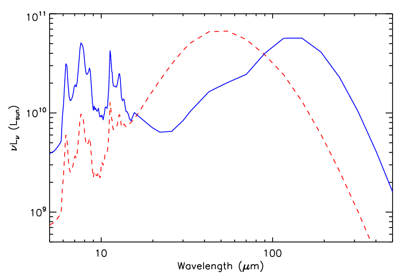
We see that the rest-frame 70 m luminosity is the best tracer of the total infrared luminosity. This means that, for a given infrared luminosity, the scatter of is the smallest. This can easily be understood by considering the two extreme templates shown in Fig. 12. The two templates are normalized to have the same total infrared luminosity, and we see that the rest-frame 70 m luminosity minimizes the scatter because it is close to the intersection of the two templates (between 80 and 90 m). The same argument also explains why the 8 and the 24 m luminosities are the worst tracers of
These correlations were derived based on a far-infrared (160 m) selected sample of galaxies, which will introduce some biases. For general use, we recommend the more general relations developed in the next section, even if the differences are small.
4.2 Validation with higher redshift sources
The sample from which we derived the correlations Eq. (4) is dominated by moderate redshift galaxies (93% lie at ) with direct far-infrared detections. In order to probe higher redshifts for a given infrared luminosity, we make use of the measurements from our stacking analysis (Fig. 5). For example, galaxies with are directly detected up to , but the stacking points probe . Fig. 7 shows the luminosity correlations including both the individually detected galaxies and the stacking analysis data. While the general agreement is good, there are small systematic shifts between the two samples. This is probably explained by selection effects. For example, at a given 24 m rest-frame luminosity, the stacking method allows us to detect galaxies with lower 160 m luminosities than the direct detections, and thus includes sources with lower infrared luminosities. Equivalently, galaxies selected at 24 m are warmer than galaxies selected at 160 m. This hypothesis is confirmed by the simulations presented in Appendix B.

If we recompute the correlations including the stacking data, giving each stacking point an additional weight equal to the square root of the number of stacked sources, we find that
| (6) |
These correlations, plotted using solid lines in Fig. 7, show small changes from the results for 160 m-selected galaxies in Eq. (4). These new relations are representative of the total infrared galaxy population, as the full sample includes all types of galaxies (i.e. warm and cold, corresponding to mid- and far-infrared selection, respectively) over a broad range of redshifts. In particular, they are reliable up to for LIRGs and for ULIRGs.
Note that the scatter in the relations at 24 m increased by far more than the scatter at the other wavelengths. We are uncertain as to the cause. While we think AGN contamination in the sample is small, it could cause part of the increase. It may also be due to extra systematic scatter in the K-corrections for sources at when the PAH features start to enter the 24 m band.
4.3 Uncertainties from the integration of the SED and the K-correction
The systematic uncertainties in these relations arise from uncertainties in our estimate of and any errors in the K-corrections.
We showed in Fig. 3 that the errors in the estimate of can be quite large at high redshift (for example 30% at redshift ). But these large errors are only found for the coldest (i.e. less luminous) templates of the Lagache et al. 2004 library and these quiescent galaxies do not seem to be representative of the distant universe. More realistic templates, with a typical luminosity of from observed luminosity functions (Le Floc’h et al. 2005; Caputi et al. 2007) at these redshifts show much smaller errors (about 15%, see the dark area on Fig. 3). Thus, we estimate that the systematic uncertainties in are less than 15% for redshifts and less than 20% for redshifts up to . As most of the galaxies in our sample lie at , such small uncertainties will have little effect on the estimated correlations.
| 8 m | 24 m | 70 m | 160 m | |
|---|---|---|---|---|
To obtain the rest-frame luminosities for each band, we have to compute and apply a K-correction, which is derived from template fits to the data. The choice of the model was already seen in §3.2 to have little effect (less than 25% for and less than 10% for ). Tab. 4 shows the luminosity-dependent changes in the correlations if we use the Chary & Elbaz 2001 models instead of the Dale & Helou 2002 models to compute the K-correction. Systematic uncertainties found for typical starbursts, LIRGs and ULIRGs are generally less than 10% at 24, 70 and 160 m and modestly larger (15%) at 8 m.
4.4 Useful relations to estimate
In the last few sections we have shown that the knowledge of one infrared flux between 8 and 160 m can provide a very reasonable estimate of the total infrared luminosity and hence of the star formation rate. In this section we explore whether combining several monochromatic luminosities can significantly improve the estimates. We fit the infrared luminosity as a sum of power-law relations for each wavelength,
| (7) |
where the coefficients and slopes are free parameters. We fit the data, including the stacking results, using combinations of two wavelengths, three wavelengths or all four wavelengths, as summarized in Tab. 5.
| Number of bands | 1- | ||||||||
| 1 band | 377.9 | 0.83 | 37 % | ||||||
| 6856 | 0.71 | 54 % | |||||||
| 7.90 | 0.94 | 19 % | |||||||
| 4.24 | 0.98 | 31 % | |||||||
| 2 bands | 5607 | 0.71 | 1.50 | 34 % | |||||
| 1.27 | 12.62 | 0.92 | 20 % | ||||||
| 3.87 | 0.96 | 1.58 | 0.95 | 11 % | |||||
| 3 bands | 0.0071 | 1.11 | 1.28 | 12.8 | 0.92 | 19 % | |||
| 1.62 | 0.99 | 1.59 | 0.98 | 3.78 | 0.94 | 7 % | |||
| 4 bands | 8.86 | 0.81 | 1.28 | 1.00 | 1.45 | 0.98 | 3.92 | 0.94 | 6 % |
Obviously, when we use more than one monochromatic luminosity, we get a more accurate estimate of . For example, estimating the infrared luminosity from the 8 and 24 m luminosities leads to a scatter about the resulting correlation of only 34% instead of the 37% and 54% found for the individual luminosities. Using the three far-infrared bands or all four bands give very accurate results, scatters of 7% and 6% respectively, both because the infrared emission is dominated by emission from large grains that peaks between 80 and 150 m and becuase these linear combinations can closely approximate our method for constructing from the data. Once the scatter is significantly smaller than , the uncertainties are dominated by systematic errors.
Such empirical relations may be very useful in practice for measuring the total infrared luminosity of infrared star-forming galaxies from limited data. In particular, mid-infrared fluxes (8 and 24 m) are particularly easy to obtain for large numbers of sources and are well-suited for estimating and conducting statistical studies of star formation in LIRGs and ULIRGs. Moreover, the estimates are nearly independent of the choice of a model, so it is easy to obtain relatively precise estimates for the infrared luminosity of starburst galaxies (30% 1-) without any strong assumptions.
4.5 Comparison with previous studies

Figure 8 compares our correlation (Eq. 6) between the 24 m luminosity and to earlier results from Sajina et al. 2006 and Takeuchi et al. 2005. The Sajina et al. 2006 sample consists of ISO FIRBACK sources selected at 170 m and the Takeuchi et al. 2005 sample was mainly selected at 100 m because they required sources to be detected in all four IRAS bands (12, 25, 60 and 100 m). As suggested by Sajina et al. 2006, the difference between these two results can be attributed to selection effect, with IRAS-selected sources being warmer than ISO sources. This effect is similar to the one we discussed in Sect. 4.2 and provide details for in Appendix B. Our correlation is roughly bounded by the relations from Takeuchi et al. 2005 and Sajina et al. 2006 – the warmest galaxies in our sample (the stacking points) agree well with the relation of Takeuchi et al. 2005, while the coldest points are in better agreement with the prediction of Sajina et al. 2006. We are sampling a wider range of temperature than these previous studies because of our broader selection criteria. Finally, Dale & Helou 2002 also tried to estimate the total infrared luminosity based on a linear combination of the three MIPS monochromatic luminosities. If we estimate using their relations we find good agreement, with a systematic shift of only 6% and an rms scatter of 6%.
5 Evolution of galaxies and application to the High-Redshift Universe

5.1 Application to the High-Redshift Universe
Perfect measurements of the infrared luminosity of high redshift galaxies requires well-sampled, rest-frame infrared SEDs. Unfortunately, obtaining such data is very observing-time consuming because of the relatively low sensitivity of far-infrared data. Moreover, at high redshift, the maximum of the infrared emission which is due to emission by big grains is redshifted to submillimeter wavelengths. In order to study star formation at high redshift, we need to estimate the total infrared luminosity with as few parameters as possible. Our study shows that the total infrared luminosity can be well constrained from the 8 or 24 m rest-frame luminosities (with uncertainties of 37 and 54% respectively) and that combining these two luminosities gives a modestly better estimate (uncertainties of 34%). Caputi et al. 2007 used our conversion between the rest-frame 8 m luminosity and the to determine the bolometric infrared luminosity function at . They show that 90% of the infrared energy density due to star-forming systems is produced equally by LIRGs and ULIRGs, while LIRGS dominate the emission at . A more accurate estimate of can be obtained given the 70 m luminosity, with a scatter of only (1-). It will be very interesting to test whether these relations hold for the individually detected, faint far-IR sources that will be found in ongoing ultra-deep 70 m surveys (Frayer et al. 2006, e.g.).
5.2 Evolution of SEDs?
As our galaxies span a wide range of infrared luminosities and redshifts, it is interesting to investigate whether we observe any evolution within our sample.

Figure 9 compares the rest-frame 24/8 and 160/70 infrared colors of our low redshift, directly detected galaxies to those of the stacked galaxies at higher redshifts. The color traces the balance between PAHs and Very Small Grains (VSGs), while the color is set by the temperature of the big grains. In this rest-frame color-color diagram, all the high redshift points are compatible with the lowest redshift sources, which suggests that there is little evolution in the dust content of infrared galaxies between (which is the median redshift of our sample of directly detected galaxies) and . If we compare the data to the predictions of several SED models (Lagache et al. 2004; Dale & Helou 2002; Chary & Elbaz 2001), we find the templates of Dale & Helou 2002 show the best agreement with the data. The Lagache et al. 2004 starburst model underestimates both colors, probably because it over estimates the dust temperature, and the Chary & Elbaz 2001 model gives intermediate results. These differences are related to the discussions of these templates in Sect. 3.2 and Fig. 4. The differences are not a consequence of our template choice – computing the K-corrections using the other templates produces similar rest frame colors for the data and similar levels of agreement between the models and the data (see Appendix C).
5.3 Far-infrared vs Submillimeter galaxies


Figure 9 also shows that the 160/70 color decreases with increasing galaxy luminosity, which means that the brightest galaxies are the warmest. This well known property of infrared galaxies (Soifer et al. 1987, e.g.) is also reproduced by the models.
In Fig. 10 we examine the evolution of the relationship between dust temperature and with redshift. We have, effectively, three redshift bins: a low redshift sample made up of the 372 directly detected galaxies, an intermediate redshift sample corresponding to the 8 stacking points from the Boötes field (red squares) and the high redshift sample consisting of the 5 stacking points from the CDFS and HDFN (purple stars). Figure 10 shows that there is no significant evolution in the relationship between and the dust temperature with redshift. All the data lie in the same region, even if we observe some small differences between the stacking points and the directly detected galaxies. At low luminosity (), the stacking points are warmer than the sources directly detected in all bands, while the reverse is seen at higher luminosities. This should be interpreted as a selection effect, as we confirm with the simulations presented in Appendix B.
We can also compare the relation between dust temperature and total infrared luminosity with other published samples of SMGs and AGNs (Fig. 11). Radio and submillimeter data probe the coldest dust component. In order to compare our results with longer wavelength surveys, we have to estimate the temperature of the cold dust component. We used the Dale & Helou 2002 library to convert the far-infrared colors (100/60 and 160/70) into estimates of by fitting a modified blackbody to the templates between 100 and 500 m. We find typical temperatures in the range of 18-30 K. Yang et al. 2007 and Yang & Phillips 2007 found higher dust temperatures for the same range of infrared luminosities for sources with . Their dust temperatures were determined by fitting modified black-body spectra to at least three photometric points between 60 and 850 m. We suspect they find higher temperatures because for their 60 m fluxes will be contaminated by VSG emission that biases the temperature upwards. As shown in Yang et al. 2007, the difference can also be attributed to different spatial scales of the star formation process, where higher temperatures could indicate that the star formation occurs in more concentrated regions. Figure 11 shows the relation between our estimates for and . We also include the data from Chapman et al. 2003 for local IRAS sources, where we used the same method to convert the 100/60 colors into cold dust temperatures. Their results are in good agreement with our own. We also included data from Sajina et al. 2006 (FIRBACK 170 m sources), Kovács et al. 2006 (SMGs), and Benford et al. 1999; Beelen et al. 2006 (dusty quasars).
Sub-millimeter surveys do not detect warm or low luminosity sources (Chapman et al. 2005), so the infrared and sub-millimeter analyses seem to be complementary, and by comparing the two approaches we can study whether the SMGs are a dominant or marginal population for galaxy evolution. From the previous samples we selected sub-samples consisting of the infrared galaxies in SMGs with and . These sub-samples are shown in separate panels of Fig. 11. At , we see that the two SMGs are colder than our infrared sources and that we do not detect a large population of such cold galaxies in the infrared. A small fraction of cold sources could exist and would be folded into our stacking points. At , our stacking point is in good agreement with the lowest luminosity SMGs. Unfortunately, the GOODS fields we used to build our sample are too small to include any of the higher luminosity galaxies. However, the good agreement with SMGs where they do overlap suggests that high-redshift SMGs are similar to infrared star-forming galaxies. This suggests that infrared and submillimeter/radio surveys are exploring the same source population but the methods compliment each other because the infrared is well suited for sources, while the submillimeter is better for high-redshift sources because of the advantageous K-corrections in this wavelength range.
6 Conclusions
In this paper, we have presented correlations between rest-frame 8 m, 24 m, 70 m and 160 m luminosities and an estimate for the total infrared luminosity derived without making any assumption on the shape of the SED that might bias the results. For a sample of 372 far-infrared (160 m)-selected galaxies with we found that the infrared monochromatic luminosities are strongly correlated with the total infrared luminosity and we derived relations to estimate from the monochromatic luminosities. In order to validate this result at higher redshifts, we used a stacking analysis to extend the data to fainter and higher redshift galaxies. For galaxies selected at 24 m the new data agrees well with the local sample up to a small systematic shift that we attribute to the differences in the selection criteria – on average, galaxies selected in the mid-infrared are warmer than those selected in the far-infrared. The revised correlations including both samples are probably better for general use. As expected we find that combining several monochromatic infrared luminosities yields a more precise estimate of the total infrared luminosity than using a single luminosity. Since the correlations were derived from a large number of galaxies with a wide range of luminosities and temperatures and extending to , they should hold for most star-forming galaxies. In particular, they are applicable for LIRGs up to and for ULIRGs up to . Extrapolations to higher redshifts, although not tested here, should give reasonable results. It is important to remember that all known QSOs were removed from our sample. While a similar study of AGN sample would be very interesting, we have only 7 QSOs detected in all four bads (8, 24, 70, 160 m) and cannot carry out the analysis. Our correlations should not be used for AGNs unless further tests demonstrate their validity.
Dale et al. 2005 claim that it is dangerous to use the 8 m luminosity as a tracer of the total infrared luminosity because they observed strong variations (about a factor 10) of this ratio for their sample of nearby galaxies (SINGS). However, their sample contains many different objects with very different dust properties and they examined different regions inside galaxies in detail. Our study shows that at higher redshift and on larger scales, the integrated galaxy and dust properties of star-forming galaxies are more homogeneous, and that using the 8 or 24 m luminosities to estimate the total infrared luminosity has uncertainties of between 40–50% that are much smaller than those given by Dale et al. 2005. We also compared our results at 24 m to previous studies and found good agreement. The differences we observed can be explained by differences in the sample selection criteria.
For the sample as a whole, we find no evidence for significant evolution in the far-infrared SED properties of infrared galaxies with redshift. Both the infrared colors and the relationship between dust temperature and of high redshift galaxies from the stacking analysis are compatible with the galaxies in the low redshift sample. A small evolution amount is not detectable because we used different selection criteria at low (far-infrared) and high (mid-infrared) redshifts. Finally, we compared our sample to submillimeter data and found that the cold SMGs observed at are a marginal population that is not representative of infrared star-forming galaxies. The infrared is the most powerful wavelength range to study the evolution of star-forming galaxies at because submillimeter surveys only select the coldest galaxies. However, submillimeter and radio wavelengths are more powerful for higher redshift, dusty galaxies, because they better probe the dust emission peak. Thus the two approaches complement each other for studies of galaxy dust properties over cosmic time.
Acknowledgements.
We are grateful to the anonymous referee for a careful reading of the manuscript. We also thank David Elbaz, Alexandre Beelen and Delphine Marcillac for fruitful discussions. This work is based on observations made with the Spitzer Space Telescope, which is operated by the Jet Propulsion Laboratory, California Institute of Technology under a contract with NASA.References
- Alonso-Herrero et al. (2006) Alonso-Herrero, A., Perez-Gonzalez, P. G., Alexander, D. M., et al. 2006, ApJ, 640, 167
- Beelen et al. (2006) Beelen, A., Cox, P., Benford, D. J., et al. 2006, ApJ, 642, 694
- Benford et al. (1999) Benford, D. J., Cox, P., Omont, A., Phillips, T. G., & McMahon, R. G. 1999, ApJ, 518, L65
- Caputi et al. (2006) Caputi, K. I., Dole, H., Lagache, G., et al. 2006, A&A, 454, 143
- Caputi et al. (2007) Caputi, K. I., Lagache, G., Yan, L., et al. 2007, ApJ, 660, 97
- Chapman et al. (2005) Chapman, S. C., Blain, A. W., Smail, I., & Ivison, R. J. 2005, ApJ, 622, 772
- Chapman et al. (2003) Chapman, S. C., Helou, G., Lewis, G. F., & Dale, D. A. 2003, ApJ, 588, 186
- Chapman et al. (2004) Chapman, S. C., Smail, I., Blain, A. W., & Ivison, R. J. 2004, ApJ, 614, 671
- Chary & Elbaz (2001) Chary, R. & Elbaz, D. 2001, ApJ, 556, 562
- Daddi et al. (2007) Daddi, E., Alexander, D. M., Dickinson, M., et al. 2007, Multiwavelength study of massive galaxies at z2. II. Widespread Compton thick AGN and the concurrent growth of black holes and bulges, astro-ph/0705.2832
- Dale et al. (2005) Dale, D. A., Bendo, G. J., Engelbracht, C. W., et al. 2005, ApJ, 633, 857
- Dale & Helou (2002) Dale, D. A. & Helou, G. 2002, ApJ, 576, 159
- Dole et al. (2006) Dole, H., Lagache, G., Puget, J. L., et al. 2006, A&A, 451, 417
- Dole et al. (2004a) Dole, H., Le Floc’h, E., Pérez-González, P. G., et al. 2004a, ApJS, 154, 87
- Dole et al. (2004b) Dole, H., Rieke, G. H., Lagache, G., et al. 2004b, ApJS, 154, 93
- Eisenhardt et al. (2004) Eisenhardt, P. R., Stern, D., Brodwin, M., et al. 2004, ApJS, 154, 48
- Fabricant et al. (2005) Fabricant, D., Fata, R., Roll, J., et al. 2005, PASP, 117, 1411
- Fazio et al. (2004) Fazio, G. G., Ashby, M. L. N., Barmby, P., et al. 2004, ApJS, 154, 39
- Fiore et al. (2007) Fiore, F., Grazian, A., Santini, P., et al. 2007, Unveiling obscured accretion in the Chandra Deep Field South, astro-ph/0705.2864
- Frayer et al. (2006) Frayer, D. T., Fadda, D., Yan, L., et al. 2006, AJ, 131, 250
- Gordon (2006) Gordon, K. D. 2006, in prep.
- Gordon et al. (2005) Gordon, K. D., Rieke, G. H., Engelbracht, C. W., et al. 2005, PASP, 117, 503
- Jannuzi & Dey (1999) Jannuzi, B. T. & Dey, A. 1999, in ASP Conf. Ser. 191, Photometric Redshifts and High-Redshift Galaxies, ed. R. Weymann, L. Storrie-Lombardi, M. Sawicki, & R. Brunner (San Francisco: ASP), 111
- Kennicutt (1998) Kennicutt, R. C. 1998, ApJ, 498, 541
- Kennicutt et al. (2003) Kennicutt, R. C., Armus, L., Bendo, G., et al. 2003, PASP, 115, 928
- Kovács et al. (2006) Kovács, A., Chapman, S. C., Dowell, C. D., et al. 2006, ApJ, 650, 592
- Lacy et al. (2004) Lacy, M., Storrie-Lombardi, L. J., Sajina, A., et al. 2004, ApJS, 154, 166
- Lagache et al. (2004) Lagache, G., Dole, H., Puget, J. L., et al. 2004, ApJS, 154, 112
- Le Fèvre et al. (2005) Le Fèvre, O., Vettolani, G., Garilli, B., et al. 2005, A&A, 439, 845
- Le Floc’h et al. (2005) Le Floc’h, E., Papovich, C., Dole, H., et al. 2005, ApJ, 632, 169
- Le Floc’h et al. (2007) Le Floc’h, E., Willmer, C. N. A., Noeske, K., et al. 2007, ApJ, 660, L65
- Marcillac et al. (2006) Marcillac, D., Elbaz, D., Chary, R. R., et al. 2006, A&A, 451, 57
- Papovich et al. (2006) Papovich, C., Cool, R., Eisenstein, D., et al. 2006, AJ, 132, 231
- Papovich et al. (2004) Papovich, C., Dole, H., Egami, E., et al. 2004, ApJS, 154, 70
- Papovich et al. (2007) Papovich, C., Rudnick, G., Le Floc’H, E., et al. 2007, ApJ, 668, 45
- Pope et al. (2006) Pope, A., Scott, D., Dickinson, M., et al. 2006, MNRAS, 370, 1185
- Richards et al. (2006) Richards, G. T., Lacy, M., Storrie-Lombardi, L. J., et al. 2006, ApJS, 166, 470
- Rieke et al. (2004) Rieke, G. H., Young, E. T., Engelbracht, C. W., et al. 2004, ApJS, 154, 25
- Sajina et al. (2006) Sajina, A., Scott, D., Dennefeld, M., et al. 2006, MNRAS, 369, 939
- Sanders & Mirabel (1996) Sanders, D. B. & Mirabel, I. F. 1996, ARA&A, 34, 749
- Soifer et al. (1987) Soifer, B. T., Sanders, D. B., Madore, B. F., et al. 1987, ApJ, 320, 238
- Stern et al. (2005) Stern, D., Eisenhardt, P., Gorjian, V., et al. 2005, ApJ, 631, 163
- Swinbank et al. (2004) Swinbank, A. M., Smail, I., Chapman, S. C., et al. 2004, ApJ, 617, 64
- Symeonidis et al. (2006) Symeonidis, M., Rigopoulou, D., Huang, J.-S., & Davis, M. 2006, ApJ
- Takeuchi et al. (2005) Takeuchi, T. T., Buat, V., Iglesias-Páramo, J., Boselli, A., & Burgarella, D. 2005, A&A, 432, 423
- Taylor et al. (2005) Taylor, E. L., Mann, R. G., Efstathiou, A. N., et al. 2005, MNRAS, 361, 1352
- Vanzella et al. (2005) Vanzella, E., Cristiani, S., Dickinson, M., et al. 2005, A&A, 434, 53
- Vanzella et al. (2006) Vanzella, E., Cristiani, S., Dickinson, M., et al. 2006, A&A, 454, 423
- Werner et al. (2004) Werner, M. W., Roellig, T. L., Low, F. J., et al. 2004, ApJS, 154, 1
- Wolf et al. (2004) Wolf, C., Meisenheimer, K., Kleinheinrich, M., et al. 2004, A&A, 421, 913
- Yang et al. (2007) Yang, M., Greve, T. R., Dowell, C. D., & Borys, C. 2007, ApJ, 660, 1198
- Yang & Phillips (2007) Yang, M. & Phillips, T. 2007, ApJ, 662, 284
- Zheng et al. (2007) Zheng, X. Z., Dole, H., Bell, E. F., et al. 2007, Infrared Spectral Energy Distributions of z0.7 Star-Forming Galaxies, astro-ph/0706.0003
Appendix A The K-corrections for the stacking points
| bin (mJy) | Redshift bin | 8 m | 24 m | 70 m | 160 m |
|---|---|---|---|---|---|
| 5.4% | 1.2% | 0.7% | 1.3% | ||
| 3.5% | 1.5% | 1.1% | 1.3% | ||
| 8.0% | 1.5% | 0.8% | 0.6% | ||
| 4.8% | 0.8% | 0.6% | 1.0% | ||
| 4.0% | 1.0% | 0.9% | 1.0% | ||
| 10.6% | 3.1% | 2.3% | 1.5% | ||
| 5.1% | 1.0% | 0.9% | 1.2% | ||
| 2.8% | 0.8% | 0.7% | 0.5% | ||
In Sect. 3.2 we K-corrected the stacking points using the mean redshift of the sources rather than averaging over the redshift distribution of the bin. We used simulations to test whether this simplification significantly affects our results.
For each template in the Dale & Helou 2002 library we built a mock sample with the redshift and flux distributions of our Boötes sub-samples (see Tab. 2), computing both the rest-frame and observed-frame 8, 24, 70 and 160 m fluxes for each source. We then compared the true, averaged rest-frame fluxes to the values found by averaging the observed-frame fluxes and K-correcting to the rest frame using the average redshift as we do in the stacking analysis. The results are given in Tab. 6. The differences are negligible at 24, 70 and 160 m. At 8 m, the K-corrections vary strongly with redshift because of the PAH features. As a result, the errors are larger and reach 10% for the two bins. However, these two points have such large uncertainties in our data (see Tab. 2), that even 10% correction would not significantly change our results. We conclude that using the K-correction corresponding to the mean bin redshift is sufficiently accurate for our purposes.
Appendix B Effect of the selection on the correlations
We used a simulation to understand and quantify the effects of selection criteria on the correlations presented in this paper.
We used two templates characterized by their parameter from the Dale & Helou 2002 library to model the galaxies. Dale et al. 2005 found that most galaxies have SEDs in the range so we use the two extremes of a warm template with and a cold template with . These two templates are shown in Fig. 12.
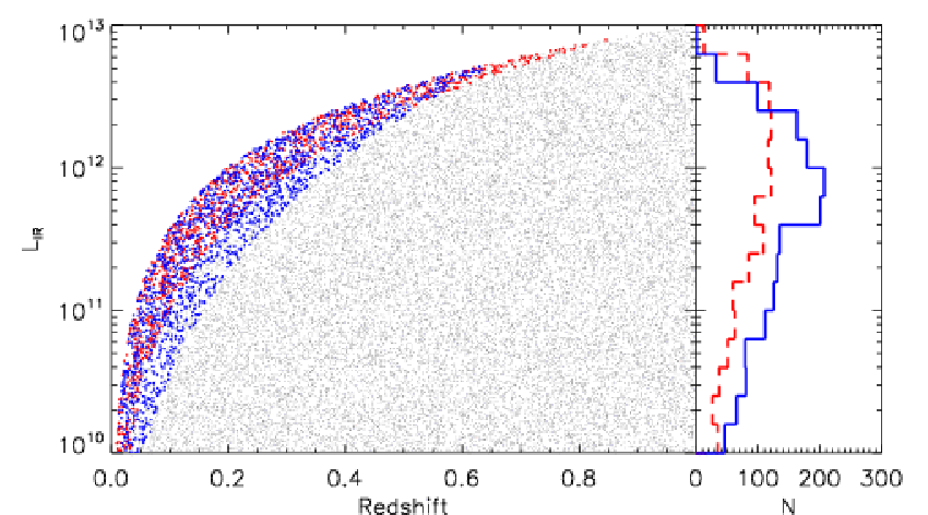
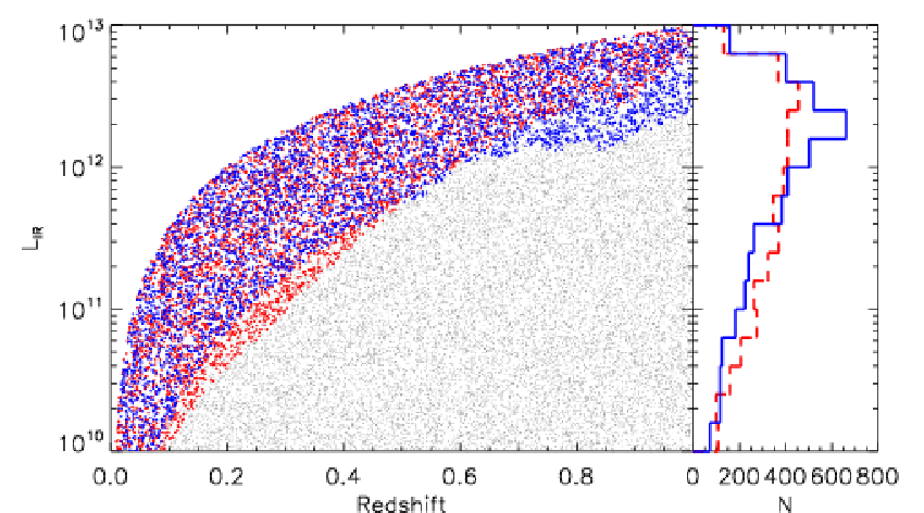
We randomly and uniformly distributed 20000 galaxies in the plane over the range , , and . The upper limit on the luminosity was determined empirically from our sample of 372 directly detected galaxies. We randomly assigned half of the galaxies to be warm and the other half to be cold and then computed the 8, 24, 70 and 160 m fluxes of each galaxy. Given a set of detection limits, we can now explore which kind of galaxies will be detectable.
In the Boötes field, the difference is between the directly detected sources and the stacked sources. The directly detected sources had to exceed flux limits of [0.006, 1, 23, 92] (mJy) at 8, 24, 70 and 160 m, respectively. The stacked sources had to be detected at 24 m (and effectively at 8 m) but for a stack of 100 sources they could be 10 times fainter in the longer wavelength bands. Thus, the stacked sources had to exceed flux limits of [0.006, 1, 2.3, 9.2] (mJy). Figure 13 illustrates the consequences of these two selection criteria on the balance between the warm and cold sources as a function of luminosity. For normal galaxies with , directly detected galaxies tend to be cold while stacked galaxies tend to be warm. For high luminosities (), we see the reverse. We probe colder sources with the stacking analysis than with direct detection. Both effects are a consequence of the warm galaxies having a higher and lower than the cold galaxies (see Fig. 12). Thus, by stacking the undetected far-infrared galaxies, we are preferentially adding warm galaxies at low luminosities and cold galaxies at high luminosities, and this explains the differences observed in Fig. 7.
Appendix C Influence of the library choice on the K-corrections

While the infrared colors of our sample are in better agreement with the predictions of the Dale & Helou 2002 model (Fig. 9), one might argue that this is a consequence of using these templates to compute the K-corrections. However, we have verified that using the Lagache et al. 2004; Chary & Elbaz 2001 libraries for the K-corrections has no effect on our conclusion. Figure 14 shows the median rest-frame colors computed with three different SED models (Dale & Helou 2002; Chary & Elbaz 2001; Lagache et al. 2004) for the 372 galaxies directly detected at all wavelengths. We clearly see that for all three K-correction models the resulting rest-frame colors of the sample are in better agreement with the Dale & Helou 2002 model predictions.