Modeling the pressure Hessian and viscous Laplacian in Turbulence: comparisons with DNS and implications on velocity gradient dynamics
Abstract
Modeling the velocity gradient tensor along Lagrangian trajectories in turbulent flow requires closures for the pressure Hessian and viscous Laplacian of A. Based on an Eulerian-Lagrangian change of variables and the so-called Recent Fluid Deformation closure, such models were proposed recently (Chevillard & Meneveau, Phys. Rev. Lett. 97, 174501 (2006)). The resulting stochastic model was shown to reproduce many geometric and anomalous scaling properties of turbulence. In this work, direct comparisons between model predictions and Direct Numerical Simulation (DNS) data are presented. First, statistical properties of A are described using conditional averages of strain skewness, enstrophy production, energy transfer and vorticity alignments, conditioned upon invariants of the velocity gradient. These conditionally averaged quantities are found to be described accurately by the stochastic model. More detailed comparisons that focus directly on the terms being modeled in the closures are also presented. Specifically, conditional statistics associated with the pressure Hessian and the viscous Laplacian are measured from the model and are compared with DNS. Good agreement is found in strain-dominated regions. However, some features of the pressure Hessian linked to rotation dominated regions are not reproduced accurately by the model. Geometric properties such as vorticity alignment with respect to principal axes of the pressure Hessian are mostly predicted well. In particular, the model predicts that an eigenvector of the rate-of-strain will be also an eigenvector of the pressure Hessian, in accord with basic properties of the Euler equations. The analysis identifies under what conditions the Eulerian-Lagrangian change of variables with the Recent Fluid Deformation closure works well, and in which flow regimes it requires further improvements.
pacs
02.50.Fz, 47.53.+n, 47.27.GsI Introduction
Fundamental understanding of universal features of the small-scale structure of turbulence has been a long-standing challenge in turbulence research K41; TenLum72; Kra74; MonYag75; Fri95; Pop00; TsinoBook. While considerable phenomenological understanding has been accumulated in recent decades, the challenge of relating observed phenomena and statistical properties to the dynamical equations (Navier-Stokes) remains unmet. The velocity gradient tensor (where u denotes the velocity vector) provides a rich characterization of the topological and statistical properties of the fine-scale structures in turbulence. Having a spectral peak at around the Kolmogorov wavelength ( is the Kolmogorov dissipative length scale), is a quantity dominated by motions in the viscous range. The antisymmetric part of the tensor is the vorticity representing small-scale rotation of fluid elements, while its symmetric part, the strain-rate tensor, represents fluid deformation rate. The Lagrangian evolution of this tensor can be described by an evolution equation that is obtained from taking the gradient of the Navier-Stokes equations. The resulting system is unclosed since it contains the anisotropic part of the pressure Hessian and the viscous term. When both of these are neglected, the system is closed (called Restricted Euler - RE- dynamics) LeoPhD; Vieille1; Vieille2; Cant1. The RE equations already predict several known geometric turbulence phenomena associated with Cant2; Ash87; Lun94; ooimar99; BosTao02; TaoKat02; Zef03; TsinoLag; GibHol07, such as preferential alignments of vorticity with strain-rate eigenvectors and preponderance of axisymmetric expansion and positiveness of the intermediate eigenvalue of the strain-rate. Neverteless, RE produces singularities in a relatively short, finite time (see Ref. TsinoBook for a review).
Phenomenologically, other phenomena such as small-scale intermittency may also be probed, by studying the probability distribution functions (PDF) of individual velocity gradient elements. For instance, it is known that the PDFs of longitudinal and transverse gradients, e.g. and in particular directions, respectively, can be described by elongated stretched exponential tails Fri95; CasGag90; KaiSre; CheCas06 or by superposition of stretched exponential bifprl. Also the moments of these gradients scale in non-trivial (anomalous) ways with the Reynolds number Nel90; sreene. Understanding such anomalous scaling behavior of turbulence is another open challenge. Therefore, the wealth of geometric, dynamical and statistical turbulence phenomena that can be described by the velocity gradient tensor, coupled with the fact that a dynamical equation (even though unclosed) is available from the gradient of the Navier-Stokes equations, makes a tensor variable of considerable interest for further study. The role of pressure in the intermittent nature of velocity gradients was also pointed out by Kraichnan in early works Kra90; Kra91.
Based on prior works Vieille2; Cant1; GirPop90; ChePum99; JeoGir03; LiMen05; LiMen06, a stochastic dynamical model for the time evolution of has been proposed CheMen06; CheMen07CRAS. The model includes a closure for the pressure Hessian, i.e. , and the viscous term, i.e. in terms of the local value of the velocity gradient tensor. The approach, reviewed in detail in §II, consists in a change of variables from Eulerian positions to Lagrangian labels before assuming isotropy in the associated gradient tensors to be modeled. The Eulerian-Lagrangian transformation involves a Jacobian matrix that is modeled using the local value of the velocity gradient tensor by using the “Recent Fluid Deformation” closure. The model system is forced using a Gaussian white-in-time random force. The resulting stochastic model consists of eight independent coupled stochastic differential equations (SDEs) that aim to describe the time evolution of each of the tensor elements of , following a fluid particle in a turbulent flow.
The results of Ref. CheMen06 show that the finite-time divergence exhibited by the Restricted Euler system is regularized with the inclusion of the proposed models for pressure Hessian and viscous term. And, with the random forcing, stationary statistics of the velocity gradient tensor are obtained, with realistic statistical properties such as preferential alignment of vorticity and the preferential state of axisymmetric expansion. The shape of probability distribution function of longitudinal and transverse gradients is quite realistic and even some well-known properties of anomalous scaling in turbulence are reproduced CheMen06; CheMen07CRAS. A limitation of the model is that at high Reynolds numbers the resulting distribution functions became increasingly unrealistic. One approach to remedy this problem has been explored BifChe07 by constructing a multi-scale version of the model, i.e. a matrix shell model that describes the velocity gradient tensors in various shells at different scales. The closure for the inter-scale interaction terms is based on the criterion that the total kinetic energy must be preserved by the modeled quadratic inter-scale interaction terms. The introduction of non-local (in scale) interactions leads to a structure of the model that is more difficult to analyze theoretically, but it provides an interesting connection between the gradients’ evolution at various scales and the energy cascade mechanism. While the matrix shell model successfully eliminates the problems at high Reynolds numbers, it does not make an explicit connection with the physics of the pressure Hessian. At this stage, then, it is of interest to further improve our understanding of the fundamental properties of the closures proposed in CheMen06, developed from the expression of pressure Hessian and viscous term as given from the Navier-Stokes equations, within the range of Reynolds numbers in which the model of CheMen06 works well.
In §III various model predictions of statistical and geometric properties of A beyond those already studied in CheMen06 are compared with Direct Numerical Simulation (DNS) at a moderate Reynolds number (). The model is evaluated using statistical measures already studied in ChePum99 in the context of the “tetrad model”. These measures include conditional averages of the “dissipation” (, where S is the symmetric part of A) and of the “enstrophy” (i.e. , where is the antisymmetric part of A). Then, a similar analysis is performed with the enstrophy production and the strain skewness. The conditional averages are expressed in terms of the two principal invariants of A, namely and . Different regions in the “-plane” have distinct physical interpretations Cant1; Cant2; ChoPer90; ooimar99 and the behavior of the computed conditional averages in these different regions thus provide useful and statistically meaningful insights into the performance of the model in dynamically very different regions of the flow.
In order to quantify and understand the average local evolution of the turbulence dynamics in the -plane, the probability current of the joint probability density is also studied in §IV. These statistics depend explicitly on both pressure Hessian and viscous Laplacian, and thus the effect of the proposed closures for these terms may be compared with the real effects obtained from the DNS.
In §V the preferential alignement of vorticity with eigendirections of both pressure Hessian and the symmetric part of the viscous Laplacian are studied in detail. Connections with theoretical results pertaining to the Euler equations are also made. Finally, in §VI the results are summarized and conclusions are presented.
II Theoretical background
II.1 Lagrangian description of the velocity gradient tensor
A description of small-scale structure of turbulence based on the velocity gradient tensor begins by taking the gradient of the Navier-Stokes equation. One then obtains the system:
| (1) |
where stands for the Lagrangian material derivative (i.e. ), the pressure divided by the density of the fluid and the kinematic viscosity. Because of incompressibility, A must remain trace-free, i.e. . Equation 1 is not closed in terms of A at the position x and time . This can be easily seen noting that the pressure field is the solution of the Poisson equation which shows that pressure is highly non-local. And the viscous term requires the Laplacian of A which is not known simply in terms of A.
As already mentioned in §I, neglecting pressure Hessian anisotropy and viscous effects leads to finite time singularities because of the strong and unopposed effects of the self-streching term . One can find in the literature several efforts at regularizing this finite time divergence, while keeping the exact self-streching term. Firstly, Girimaji and Pope GirPop90 succeded to do so by constructing a stochastic model with an imposed constraint. This constraint is imposed by modifying the non-linear term so that the pseudo-dissipation PopChe90 is lognormal with a prescribed mean and variance. Intermittency trends are put in explicitly, by prescribing a known variance of as function of the Reynolds number.
More recently, two groups proposed the idea that the local geometry of the accumulated fluid deformation, i.e. formally the Cauchy-Green tensor, may represent the missing information which allows to regularize the RE divergence. Accumulated fluid deformation thus has been used to model the pressure Hessian in the so-called “tetrad model” of Chertkov, Pumir and Shraiman ChePum99; NasPum05; NasPum07. A similar idea from Jeong and Girimaji JeoGir03 has been used to model the viscous part of Eq. (1), explicitly using the Cauchy-Green tensor. Whether or not the finite time divergence is regularized, the direct use of the Cauchy-Green tensor is limited by the fact that this tensor is fundamentaly non-stationary, i.e. as time evolves it maintains memory of the initial condition. Hence the resultant models for pressure Hessian and viscous term are intrinsically non-stationary and depend on the initial condition chosen to initialize the material deformation tracking. In the following sections, we discuss these issues in more detail and also review the simplified model of CheMen06 that avoids these problems of non-stationarity.
We also point out an alternative approach cantwell01 that renormalizes the time variable in RE dynamics so as to relegate the finite time singularities to infinite time.
II.2 Lagrangian mapping and Cauchy-Green Tensor
Following Refs. MonYag75; Con01; MajBer02, one may define a mapping between Eulerian and Lagrangian coordinates:
| (2) |
where denotes the position at a time of a fluid particle which was at the position at the initial time . Given the initial position of a fluid particle, this mapping (Eq. (2)) is fully defined at any time by
| (3) |
A quantity of much interest in continuous mechanics is the deformation gradient tensor D, defined as , which relates the variation of the position of a particle when one slightly changes the initial position. Differentiating Eq. (3) with respect to , one gets the time evolution of D, i.e.
| (4) |
and one can show MonYag75; MajBer02 that the Jacobian of the mapping , i.e. , is equal to unity at any time by virtue of incompressibility, stating that this mapping is always invertible. Eq. (4) can be exactly solved using the product integral DolFri79 or alternatively, the time-ordered exponential ItzZub80; FalGaw01
| (5) |
The Cauchy-Green tensor, , is defined as the symmetric tensor and its eigenvalue and eigenvector system describes the rotation and deformation of initially isotropic-shaped fluid volumes into various shapes as time goes on. The transport equation of the Cauchy-Green tensor can be obtained in straightforward fashion TruNol92 from Eq. (4):
| (6) |
Based on the properties of C, studies of isotropic and homogeneous turbulence in both numerical GirPop90Num and laboratory TsinoLag; TsinoBook flows have shown that cigar (one large and two small eigenvalues of C) and pancake (two large and one small eigenvalue) shapes are the most common shapes of fluid deformation.
II.3 Fluid deformation, and pressure Hessian models
Let us first remark that the pressure Hessian is not among the most studied objects in the turbulence literature (although, see Ref. NomPos98). One reason perhaps is that it cannot be described naturally from a standard transport equation along a Lagrangian trajectory. Instead, the pressure Hessian is related to the spatial distribution of the velocity gradient using singular integral operators Ohk93; OhkKis95; MajBer02:
| (7) |
where the integral is understood as a Cauchy principal value (P.V.) and is the Hessian of the Laplacian’s Greens function, namely
| (8) |
One can see from Eq. (7) that only the isotropic part of the pressure Hessian is purely local (the first term of the RHS of Eq. (7)). All the nonlocal effects of pressure Hessian enter through the anisotropic part (or deviatoric part corresponding to the second term of the RHS of Eq. (7)). Hence, in this view, the RE approximation can be understood as the neglect of all the nonlocal effects implied by the incompressiblity condition: the corresponding Lagrangian particle evolves with the flow completely independent from its neighbors. As far as we know, the tetrad model ChePum99 is the first model to have been proposed for the anisotropic (i.e. nonlocal) part of the pressure Hessian. While the authors introduced the model using the language of multipoint dispersion of particles that define an evolving tetrad shape, a simple interpretation of the model can also be given in terms of the deformation and Cauchy-Green tensors.
To begin, one can re-express various Eulerian quantities such as the pressure Hessian and the viscous term in terms of Lagrangian coordinates, i.e. in terms of the fluid particle’s position at some initial time , X. For the Hessian tensor of the pressure at the current point and time one may write
| (9) |
The second term entering in the RHS of Eq. (9) requires the knowledge of the spatial distribution of the (inverse) deformation gradient, through its spatial derivative. As will be seen later, the adopted approach neglects short-time variations in the velocity gradient and in the context of the proposed Lagrangian model, it is natural to neglect spatial fluctuations of the deformation gradient, i.e. . Next, we discuss the remaining term of the RHS of Eq. (9). The fourth-order tensor can be solved along its trajectory using the dynamical evolution for the deformation tensors (Eq. (4)). For the remaining factor, the Lagrangian pressure Hessian , we choose the simplest assumption, namely the isotropic assumption:
| (10) |
Physically, this assumption states that as time progresses, one looses memory about the relative orientations of the initial locations X as far as the present value of pressure is concerned. The contraction between and then connects the model to the Cauchy-Green tensor introduced in the preceding section.
So far the pressure Hessian can then be rewritten, using Eq. (10), according to
| (11) |
II.4 Fluid deformation and modeling the viscous Laplacian
In a similar fashion, following Ref. JeoGir03, this procedure can be applied to the viscous Laplacian entering in the gradient of the Navier-Stokes equation (Eq. (1)), i.e.
| (13) |
The resulting Lagrangian Hessian of A entering in Eq. (13) will be considered as (i) isotropic, i.e. and (ii), its trace will be modeled by a friction term, i.e. . The characteristic length scale reflects the typical length in the Lagrangian frame over which A is correlated. To estimate this length-scale, we note that the typical decorrelation time of A along its Lagrangian trajectory is known to be on the order of , the Kolmogorov time-scale (where is the dissipation rate) TenLum72. During that time, a fluid particle is advected by the turbulence over a distance of the order of , where is the root mean square velocity (chosen as advective velocity scale) and the Taylor microscale. Finally, recognizing that , where is the integral time scale, one then obtains the following model for the viscous term:
| (14) |
This model is similar to the one obtained by Jeong and Girimaji JeoGir03 but using a different, more physically motivated time scale.
II.5 Stochastic model based on the Recent Fluid Deformation (RFD) closure
The various terms entering in the rhs. of Eqs. (12) and (14) include the tensor C. If this tensor is obtained from its transport equation (Eq. (6)) subject to the natural initial condition , then the closures for pressure Hessian and viscous term depend strongly on the initial time , or equivalently, on the initial position X. Due to the dispersive nature of turbulent flow, C continues to evolve with exponentially growing and decreasing eigenvalues. Instead of solving for C from its transport equation and having to deal with the problems associated with non-stationarity, in CheMen06 a simple closure was proposed. It consists of a sort of ‘Markovianization’ of the dynamics of C in that it is assumed that C evolves in a frozen velocity gradient tensor field during a characteristic (short) time . The value of A during that time is taken as the most recent value (i.e. the current, local, value). And the time-scale chosen is the typical de-correlation time-scale of A during its Lagrangian evolution, which is known to be of the order of the Kolmogorov time-scale, . Thus, the initial time is taken to be at , which allows to write in a simple way the time ordered exponential entering in Eq. (5). We thus replace the true Cauchy-Green tensor by a new tensor, called the “recent Cauchy-Green tensor’ that can be expressed in terms of simple matrix exponentials:
| (15) |
This leads to an explicit A-dependent model for the full pressure Hessian:
| (16) |
and for the viscous Laplacian
| (17) |
Inserting Eqs. (16) and (14) into Eq. (1) and writing the equation in the Itô’s language of stochastic differential equations KloPla92 the full model for the time evolution of the velocity gradient reads
| (18) |
The stochastic time evolution of the velocity gradient tensor A (Eq. 18), as proposed in Refs. CheMen06; CheMen07CRAS, relates the joint deterministic action of the self-streching term , the pressure Hessian (Eq. 16) and the viscous term (Eq. 17). Moreover, the system is forced with a stochastic Gaussian noise. The deterministic part provides two time scales: a small time scale and a large one . The latter arises in modeling the viscous diffusion term when combining the viscosity with the Taylor-microscale, which in turn is related to the large-scale velocity rms. Hence, the deterministic part gives the dependence on the Reynolds number to the model through the ratio , according to classical Kolmogorov dimensional arguments Fri95. Dependence on the Reynolds number of higher order moments of velocity derivatives (i.e. anomalous scalings and the intermittency phenomenon) have been studied and quantified in Ref. CheMen07CRAS. The purpose of this article is to focus on a single Reynolds number and to compare it with a DNS flow (see next paragraph).
The term W is a tensorial delta-correlated noise term that has been added in order to represent possible forcing effects, e.g. from neighboring eddies CheMen06; CheMen07CRAS. In Appendix A, we describe this noise extensively, and propose a way to simulate it.
II.6 DNS data and comparisons with the model
In the following, we will make extensive use of a standard direct numerical simulation (DNS) of the Navier-Stokes equation for a Taylor based Reynolds number of order . Pseudo-spectral simulations are performed, of an isotropic turbulent flow in a box using nodes. Fourier modes in shells with are forced by a term added to the Navier-Stokes equations, which provides constant energy injection rate . The viscosity of the fluid is . The time step is chosen adaptively to ensure the Courant number , where is the maximum velocity and is the grid size. In order to make comparisons between DNS data and the model, one has to specify a value for the parameter of the model . At , it has been estimated by Yeung et al. YeuPop06JoT that the ratio of the Kolmogorov scale and the integral (i.e. velocity correlation time scale) time scale is . Thus, in the following, DNS data will be compared to the model run with . Without loss of generality, the integral time scale will be set to unity. It corresponds to set time as units of . The model as written out as in Eq. (18) is solved numerically, with the parameter , using a second order predictor-corrector method (see Ref. KloPla92) with a time step of . One obtains time-series of all of the components of the tensor A that display temporally stationary statistics. In this article, we have worked with a time-series of length in units of the integral time scale . These can then be directly compared to DNS results. Furthermore the model provides statistically stationary time-series for both pressure Hessian and viscous Laplacian that can be also directly compared to DNS data.
III Conditional statistics of the velocity gradient tensor

We are interested here in studying various properties of the velocity gradient tensor conditioned upon the value of its two invariants and defined earlier. The joint probability density of (the -plane) has been studied in the past ChoPer90; Vieille2; Cant1; Cant2; ooimar99 and can be used to characterize the frequency of occurrence of the various local topologies of the flow.
For instance, in a simple way, the second invariant
| (19) |
can be understood as the competition between enstrophy ( denotes vorticity) and dissipation (per unit viscosity). Then, positive represents rotation-dominated regions and negative dissipation-dominated regions. Analogously, the third invariant
| (20) |
represents competition between enstrophy production, entering in the enstrophy evolution TsinoBook; RosMen06, i.e.
| (21) |
and the dissipation production (or Strain skewness ChePum99) entering in the dissipation evolution , i.e.
| (22) |
Let us remark that one may interpret the RQ plane in a different way, based on the eigenvalues of A (two of them can be the complex conjugate) and the zero-discriminant line (i.e. the “Vieillefosse” line, namely ). See for instance ChoPer90; Cant1; Cant2.
III.1 The joint PDF in the RQ-plane

We show in Fig. 1 the joint PDF of and , or equivalently the joint PDF of the non-dimensionalized invariants and , for both DNS and the model (Eq. (18)). In order to compute various conditional averages, a range of values of the two non-dimensionalized invariants and of A is discretized in 25 equally spaced bins. For the DNS, one observes the predominance of the Enstrophy-Enstrophy production quadrant ( and ) and the Dissipation-Dissipation production quadrant ( and ). The predominance of these two quadrants has been observed before in the literature Cant2. The model reproduces these basic trends fairly accurately, with the characteristic “tear-shape” elongation along the “Vieillefosse tail” in the Dissipation-Dissipation production quadrant. But one also observes that the model overestimates the total probability in the Enstrophy-Dissipation production region (i.e. and ) and underestimates the Dissipation-Enstrophy production region (i.e. and ). It will be shown later that this is caused by limitations in how the pressure Hessian is closed and modeled.
Next, we check whether or not dissipation (resp. enstrophy) is dominantly associated with the and (resp. and ) quadrants. Following the approach already used in ChePum99 we present in Fig. 2 the conditional averages of dissipation, i.e. and enstrophy on and . Averages are weighted by the joint density to ensure that the sum over all possible values of and gives the averages of respectively dissipation and enstrophy. We clearly see that the quadrants ; (or ; ) are dominated by dissipation (or enstrophy, respectively). The model reproduces these conditional averages quite accurately.
III.2 Enstrophy production, Strain Skewness and Energy transfer

A similar study is performed with the various quantities entering in the definition of the third invariant (Eq. (20)), namely the enstrophy production and the strain skewness ChePum99. In Fig. 3 (a) to (d) these various quantities are shown, together with the predictions from the stochastic model. In all cases, it is apparent that model predictions are quite accurate. We see also that enstrophy production is clearly dominant in the and quadrant. Let us mention that in the enstrophy-dissipation production dominated region ( and ), entrophy production becomes weakly negative, stating that in this region, enstrophy decreases with time (see Eq. (21)). Also, in Fig. 3 (a-b), we see that strain skewness is dominating in the bottom-right quadrant, but remains very important in the top-left quadrant. This is mainly linked to the fact that the evolution of dissipation not only depends on the strain skewness (or dissipation production), but also on enstrophy production, and a term linked to the pressure Hessian (see Eq. (22)).
A related quantity of interest is
| (23) |
which describes the time evolution of the pseudodissipation in the RE approximation. This quantity is sometimes called “energy transfer” Eyink95; BorOrz98; ChePum99 when A is defined by filtering in the inertial range in the context of large eddy simulations (see MenKatRev). While here A is not filtered and therefore no such direct physical interpretation is available, this quantity is still presented as additional documentation of the properties of A. Results are displayed in Fig. 3(e-f). Once again, the model reproduces well the trends observed in DNS, including negative regions in the top-right quadrant.
III.3 Geometric alignments of vorticity with strain-rate eigenvectors
An important universal feature of fully developed turbulent flows is the preferential alignment of vorticity along the eigendirection of the intermediate eigenvalue of the strain-rate tensor S (see TsinoBook and references therein). To study the alignment properties of vorticity conditioned on various values of and the plane is divided into four regions related to the eigenvalue structure of A. Instead of the line to separate high and low rotation regions as was done in the qualitative discussions of the previous sections, we now use the quantitatively more precise classification, in which the plane is divided into high and low rotation regions by the zero-discriminant line, i.e. .

Fig. 4 shows the PDF of the cosine of the angle between vorticity and eigendirections with the most negative (a-b), intermediate (c-d) and most positive (e-f) eigenvalue of the stress, for both DNS and the model. The different symbols denote the results obtained in separate quadrants as separated by the Vieillefosse (i.e. zero discriminant) and the lines. In Fig. 4(g-h) is displayed the unconditional PDF independent on the quadrant, i.e. as obtained in all regions. As already observed in CheMen06, the model predicts accurately the preferential alignment with the intermediate eigendirection (solid line), a trend of being orthogonal to the most contracting direction (dashed line), and an almost entirely decorrelated trend with the most extensive eigendirection (dash-dotted line). The agreement between DNS and the model is excellent in all cases, even when conditioning on the separate quadrants. It is interesting to note that in (a) and (b), as well as in (e) and (f), the alignment PDF is essentially the same in three quadrants but very different in the and quadrant. In Fig. 4(a) and (b) we observe that while the vorticity is mostly perpendicular to the most contracting eigendirection, in the top-right quadrant the vorticity is in fact not orthogonal to the contracting eigen-direction. This is the “vortex contracting” quadrant with an unstable focus and one contracting direction. This would suggest that the vorticity is aligned with the contracting direction. There is instead no strong preferred alignment but there is an almost zero probability that the vorticity is perpendicular to the contracting eigendirection. But, on average, when taking into account all the possible values for and , (Fig. 4(g-h)), vorticity remains weakly orthogonal to this eigendirection. In terms of the alignments with the intermediate eigendirection, one may have expected the preferential alignments to come mainly from the bottom-right quadrant as predicted by the asymptotic diverging state of the RE equations Vieille2; Cant1. Nevertheless, in Fig. 4(c) and (d) we observe instead that the alignment with the intermediate eigendirection occurs quite independently of the characteristic values in the plane. In Fig. 4(e) and (f) we observe that the alignment with the most extensive strain-rate eigendirection is random in all quadrant except, again, in the top-right quadrant where and . Vortex “contraction”, when it happens, appears to occur because it is mostly orthogonal to the extensive direction and also ‘not orthogonal’ to the contracting direction, rather than being preferentially aligned with the contracting direction. The stochastic model predicts these non-trivial statistical geometric behaviors quite well.
IV Pressure Hessian and Viscous term
Let us now focus directly on the terms requiring closure, namely the pressure Hessian and the viscous term, instead of the statistics of the velocity gradient tensor considered in the previous section. One option could be to compare individual realizations of the model terms with the corresponding DNS values along Lagrangian trajectories. However, since these terms fluctuate greatly in the DNS, a statistically more robust comparison is performed using conditional averages, conditioned on and .
IV.1 Probability current and conditional averages

The approach used in Ref. BosTao02 is followed, based on a Fokker-Planck equation for the dynamics of and . To summarize the approach, we notice that along a Lagrangian trajectory, appropriately contracting (1) with A and , using the Cayley-Hamilton theorem Cant1, one can show that the time evolution of the invariants and are given by
| (24) |
| (25) |
where is the strain variance and the non-dimensional time. Also, stands for (minus) the deviatoric part of the pressure Hessian, i.e.
| (26) |
and is the viscous term (recall that in the RE approximation, ). The Fokker-Planck equation describing the time evolution of the joint density may be written as Ris84:
| (27) |
where the divergence of the probability current controls time variations of the joint probability density . The probability current can be written in terms of conditional averages as
| (28) |
It can be decomposed into , with
| (29) |
which describes the deterministic (closed) part of the evolution of the two invariants,
| (30) |
describing the pressure Hessian effects on the evolution of and and finally,
| (31) |
describing the effects of the viscous term. An additional current might be considered in this description, linked to an additional forcing term that has been neglected in the Navier-Stokes equations (Eq. (1)). This forcing is indeed negligible in front of the other terms of the rhs. of Eq. (1) since it can be written as the (small-scale) gradient of the large-scale forcing of the velocity, and thus, we will neglect its associated probability current.
Conversely, in the Fokker-Planck equation (Eq. (27)) for the joint probability distribution of and obtained from the model (Eq. (18)), one has to take into account another term which comes from the delta-correlated Gaussian forcing. Appendix B provides the required background needed to compute the probability flux resulting from the stochastic forcing term in our model, i.e. the diffusion terms entering in Eqs. (24) and (25). It is shown that the currents associated to the deterministic and random parts of the joint stochastic evolution of and predicted by the model (see Eq. (44)) are of the same order of magnitude.
IV.2 Results
In Fig. 5 the vector plots and associated streamlines corresponding to the various probability flux terms are presented. Both results obtained from DNS and from the model are shown.
First, as reference we present in Fig. 5(a-b) the closed RE current (Eq. (29)). As is well-known Vieille2; Cant1, the deterministic probability current pushes probabilities towards the right tail of the Vieillefosse line. Since the model predicts acurately the joint probability , agreement between DNS and the model predictions (length of vectors) is quite good because the self-streching term is taken into account exactly in the model (Eq. 18) .
The action of the pressure Hessian, given by the probability current and shown in Fig. 5(c-d), is quite interesting. From the DNS data, two main pressure Hessian effects can be observed. First, the pressure Hessian counteracts the effects induced by the RE terms since the flux goes towards the center of the RQ plane along the right tail Vieillefosse line. This feature is well reproduced by the model, with vector magnitudes of the same order. Another important effect of the pressure Hessian is that in the left half-plane, the probability current leads the probability towards the left tail of the Vieillefosse line, namely towards dissipation-enstrophy production dominated region (in lower-left direction). This feature is not reproduced by the model, which instead appears to act exclusively in vertical direction, upward in the plane, and downward in the side. This explains perhaps why the model leads to an underestimation (see Fig. 1) of the probability of dissipation-enstrophy production events (i.e. the bottom-left quadrant). At the same time, the absence of “left-ward” flux out of the enstrophy-dissipation production region (i.e. top-right quadrant) may explain why the model overpredicts the probability of events in that quadrant. A very marked feature of the DNS results is that the magnitudes of the vectors are essentially negligible in the entire vortex contraction quadrant above the right Vieillefosse line ( and ), leading to some uncertainty in the computed streamlines there.
Another main difference between DNS and model predictions is the fact that for the model, vanishes at vanishing , but not for the DNS. A general feature of the pressure Hessian model is that its deviatoric part is directly proportionnal to (see Eq. (16)). Incidentally, the same occurs in further generalizations that have been proposed by Gibbon and Holm GibHol07 (see their Eq. (5.8)), namely
| (32) |
where the scalars are undertermined and are any non-singular symmetric tensors. Once again, we can see that the deviatoric part of the pressure Hessian is still proportional to . For the sake of completeness, let us remark that at least formally, this issue does not arise in the matrix shell model of BifChe07. This is because the non-local closure terms in the matrix shell model BifChe07 are not directly proportional to since the connection to pressure Hessian and Poisson equation for pressure is not included in that approach. It would be very interesting to check if the comparison with DNS for the equivalent probability current in the matrix shell model, i.e. based on relevant portions of the quadratic nonlinear interaction terms, is better or not. Such studies are left for future work.
To more clearly isolate the behavior of the pressure Hessian near line, we study the magnitude of the anisotropic (i.e. deviatoric) part of the pressure Hessian, conditioned on the local value of . Fig. 6 shows the conditional average of the norm (square) of the deviatoric part of the pressure Hessian, i.e. , where , as a function of the local value of the invariant , for both the DNS and the model. For vanishing , the conditional average from the DNS does not vanish. As discussed before this property is not reproduced by the existing models for the pressure Hessian, namely the tetrad model (Eq. (12)), the CM06 model (Eq. (16)) and the generalized tetrad model (Eq. (32)) because all of them predict a pressure Hessian proportional to . Secondly, one can see that for the range of under consideration (i.e. ( stands for the standard deviation of ), the conditional average of behaves as (up to a positive additive constant) whereas the model predicts it to be proportional to . The fact that the model predicts a quadratic behavior can be understood from a Taylor’s development, namely leading to since . The small asymmetry in the quadratic behavior seen in Fig. 6 is caused by higher order terms entering in the expansion for the model.

In terms of the viscous term, one observes in Fig. 5(e-f) that the model reproduces the probability flux reasonably well. Consistent with the observations already made in BosTao02 the viscous effect is to push the probabilities towards vanishing and , not only along the Vieillefosse line, but everywhere. We notice that the model overpredicts the magnitudes, i.e. at this Reynolds number the model provides too strong damping but is qualitatively correct.
In Fig. 5(g-h) is shown the sum of all these terms, namely the total probability current . For the model case, another term coming from the Gaussian delta-correlated forcing (see Appendix B and Eq. (49)) has been added. The circular motion around the origin of the RQ plane has already been reported in Refs. ooimar99; ChePum99. At this point, from Fig. 5 one can observe that all the terms (self-stretching, pressure Hessian and viscous Laplacian) entering in the Navier-Stokes equations (Eq. (1)) are of the same order of magnitude (viscous Laplacian is a little bit smaller than the two other terms, but not by much). Similar conclusions can be drawn for the deterministic terms entering in the model (Eq. (18) and figs. 5(b-d-f)), although, as shown in appendix B, the amplitude of the forcing is not negligible either. Focusing on the total probability current 5(g-h), we reach the conclusion that the fact that the modeled pressure Hessian (fig. 5(d)) is not able to reproduce the probability flux towards regions as it is observed in DNS (fig. 5(c)), explains why the model over predicts regions and under predicts regions, as observed in Fig. 1. We also remark that streamlines shown in the left part of Fig. 5(h) are not significant because of the very low values of the joint probability .

V Vorticity alignments with pressure Hessian and viscous Laplacian eigendirections
V.1 Pressure Hessian
Here we focus on vorticity alignment properties along the eigendirections of the pressure Hessian. It has been derived, in the inviscid limit (Euler equations) Ohk93; GalGib97; GibHol06 that vorticity tends to be simultaneously an eigenvector of the rate of strain tensor S and the pressure Hessian. When (see Eq. (21)),
| (33) |
and taking another time derivative and using the time evolution of S (see Eq. (22)), we get
| (34) |
Following Ref. Ohk93, we then notice that if vorticity of a fluid particle continues to be an eigenvector of the rate-of-strain tensor, then it is also an eigenvector of the pressure Hessian. To see if such a trend is observed in a finite viscosity turbulent flow we will quantify the aligments of vorticity with the eigendirections of the pressure Hessian. Such an analysis based on DNS has been already performed TsinoNice; Kal06, but here the purpose is to compare results with predictions of the model.
Let us focus on alignment properties of vorticity with respect to the eigendirections of the deviatoric part of the pressure Hessian (i.e. defined in Eq. (26)). Alignment PDFs are shown in Fig. 7, presented in a similar fashion as in Fig. 4. We can see in Fig. 7(a) that vorticity is preferentially orthogonal to the eigendirection of the smallest eigenvalue, except in the top-left quadrant (i.e. and ) where the local topology is dominated by one direction of streching and a stable focus. Also in this quadrant, vorticity is preferentially aligned with the extending eigendirection. The model predicts a slightly different picture since vorticity is predicted to be also preferentially othogonal to the eigendirection except in the top-right quadrant (i.e. and ) for which local topology is dominated by one compressive direction and an unstable focus.
In Fig. 7(c-d), we focus on the pressure Hessian eigendirection of its intermediate eigenvalue. In a similar way as with eigendirections of the rate-of-strain, vorticity is preferentially aligned with this eigendirection in all the quadrants, and this is also very well predicted by the model. About the eigendirection of the largest eigenvalue, we can see that for the DNS (Fig. 7(e)) vorticity is weakly preferentially aligned with the eigendirection, except again in the top-left quadrant where vorticity is clearly preferentially orthogonal to this eigendirection. In Fig. 7(f), we can see that the model predicts most of the trends quite well in all the quadrants. For the average results over all quadrants, it can be seen in Figs. 7(g-h) that the model predicts with a fairly good accuracy the behavior of vorticity with the eigendirection of the intermediate eigenvalue (although it overpredicts the peak a little bit). In the other extremal eigendirections, the model reproduces the moderate peak at but misses the narrow peaks near alignment at .
The fact that the model reproduces very well the events for which vorticity happens to be an eigenvector of the rate-of-strain tensor can be understood phenomenologically in the following way. When vorticity is an eigenvector of the rate-of-strain, i.e. , then vorticity is also an eigenvector of the velocity gradient tensor itself, namely , since by definition . Let us notice that vorticity is also an eigenvector of with the same eigenvalue . It is then straightforward to show by induction that for any power , . For these very particular events in which vorticity is an eigenvector of the rate-of-strain, one notices than the matrix exponential entering the (inverse) recent Cauchy-Green tensor (in Eq. (15)) can be written as
| (35) |
From Eq. (35) it is easily seen that vorticity is also an eigenvector of both the recent Cauchy-Green tensor (Eq. (15)) and its inverse. For example, . Finally, since the pressure Hessian is modeled as proportional to (Eq. (16)), we can state here that the present model is such that when the vorticity is an eigenvector of the rate-of-strain, then it is also an eigenvector of the modeled pressure Hessian, the ordering of the associated eigenvalues being respected in absolute value. More precisely, if vorticity is an eigenvector of S with respective eigenvalue , then vorticity is also an eigenvector of the pressure Hessian with eigenvalue .

V.2 Viscous Term
Let us now focus on the geometrical properties of the viscous tensor, namely , appearing in Eq. (1). Let us begin with its symetric part . The present model (i.e. Eq. (18)) contains the closure for the viscous term pointed of Eq. (14) that stated that the Laplacian of A is proportionnal to A itself. In terms of eigendirections, it is assumed that both S and have the same eigendirections. Among others, alignment properties of vorticity and eigendirections of should be exactly the same as alignments of vorticity with eigendirections of S. To determine whether this is observed in DNS flows, we present in Fig. 8 PDFs of the cosine of the angle between vorticity and eigendirections of the viscous term, for both DNS (a) and the model (b). Fig. 8(b) is in fact the same as Fig. 4(h) and is reproduced here for convenience. We see clearly that the overall geometrical picture are really close between DNS and the model, and that there is preferential alignment of vorticity with the eigendirection associated to the intermediate eigenvalue of the Laplacian term as well.

Let us now focus on the antisymmetric part of the viscous term, namely . The vorticity vector is given by . The viscous term can also be written as a vector, i.e. . The model for the viscous term (Eq. (17)) implies that the angle between the vorticity and the vorticity Laplacian is fixed and equals , i.e. same direction but opposite orientation, since the model (Eq. (17)) is proportional to the velocity gradient tensor A with a negative coefficient. One may wonder if this is consistent with DNS data. We represent in Fig. 9 the PDF of estimated from the same DNS fields. Clearly we see that the two vectors share preferentially the same direction, but opposite orientation. The model is therefore consistent with the observed alignment trends of the full Laplacian of velocity gradient.
VI Conclusions
Extensive comparisons have been made between predictions of a new stochastic Lagrangian model for the velocity gradient tensor and results from DNS at a corresponding moderate Reynolds number. The model reproduces many inherent geometric and statistical properties of small-scale turbulence quite well. The statistics of alignment angles between vorticity and the principal axes of the rate-of-strain tensor are very well reproduced. The joint statistics of velocity gradient invariants and are also reproduced well. Specifically, the joint PDF’s elongation into the top-left and bottom-right quadrants observed in the DNS also occurs in the model. Some differences occur in the model in the top-right and bottom-left quadrants. In order to directly assess the action of the modeled pressure and viscous terms in a statistically robust fashion that takes into account the local topology of the flow, the probability current has been studied. The agreement between DNS and model predictions is good near the dominant Vieillefosse tail in the lower-right quadrant of the plane. However, in the dissipation-enstrophy production dominated region (bottom-left), the model does not reproduce the true dynamics and requires further developments. Finally, the alignment properties of vorticity with respect to the principal axes of the pressure Hessian tensor have been studied. The model reproduces quite well the preferential alignment of vorticity with the eigendirection associated to the intermediate eigenvalue. We elucidate the fact that in the model an eigenvector of the rate-of-strain is also an eigenvector of the pressure Hessian, and this is in fact consistent with known behavior of vorticity in the inviscid limit (i.e. the Euler equations).
This analysis has confirmed that the stochastic model is capable of predicting many non-trivial properties of small-scale turbulence as described by the geometric and statistical properties of the velocity gradient tensor. Nevertheless, there appear to be difficulties in specific regions of the flow, especially those in which the vorticity is being contracted such as in the top-right or bottom-left portion of the invariant plane. Whether these drawbacks of the model are also related to the difficulties observed when raising the Reynolds number of the flow also remains to be explored.
Acknowledgements: We thank S. Chen, R. Chétrite, G. Eyink, K. Gawedzki and Y. Li for useful discussions. L.C is supported by postdoctoral Fellowship from the Keck Fundation and C.M. by the National Science Foundation.
Appendix A Definition and implementation of tensor Gaussian forcing
In this appendix, the tensorial Gaussian forcing entering in the model (Eq. (18)) is described. It can be written as
| (36) |
where are the diffusion coefficients and is a tensorial isotropic Wiener process, whose components are such that
| (37) |
The coefficients are chosen such that the noise is consistent with a trace-free, homogeneous and isotropic tensor, of a given unit variance, namely with
| (38) |
As a consequency, longitudinal components of the noise are of variance , and for the transverse ones. Also, let us recall that the dimension of the diffusion coefficients is . If the tensor is assumed isotropic itself, then the unique solution of Eq. (38) is given by
| (39) |
with
| (40) |
Appendix B Stochastic differential equations
The basic tensorial stochastic differential equation (SDE) Eq. (18) can be written as
| (41) |
where is the drift coefficients representing the self-streching, pressure Hessian and viscous terms entering in Eq. (18) and is the forcing term described in Appendix A. The associated Fokker-Planck equation for the joint probability of the velocity gradients , of is given by
| (42) |
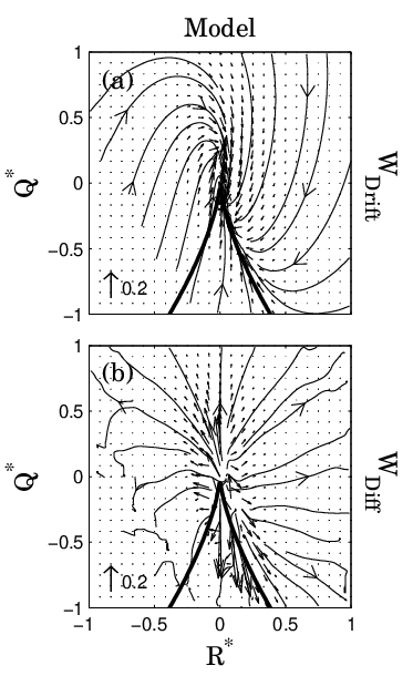
Here we are interested in the joint probability of two invariants of the velocity gradients, namely and (c.f. Eq. (27)). In Itô interpretation, both the stochastic equations governing the dynamics of and and the associated Fokker-Planck equation can be computed (c.f. GirPop90; Oks03; Ris84; KloPla92) from the evolution of A (Eq. (41)). To do so, one needs to know how a stochastic differential equation is written under a non-linear transformation since and are nonlinear functions of the components of A.
In general terms, let us call such a time dependent nonlinear transformation with components , . Starting from the SDE of A (Eq. (41)), general formula GirPop90; Oks03; Ris84; KloPla92 give the new stochastic differential equations that governes , namely
| (43) |
To compute the time evolution of the invariants and , we use Eq. (B) with the particular (time independent) nonlinear transformation and . We get
| (44) |
where, using former notations, we notice that and using the Cayley-Hamilton theorem, . Furthermore, the “spurious” drift terms coming from the delta-correlated Gaussian noise vanish, i.e. using Eq. (38) one can show that and . From a straightforward manner GirPop90; Oks03; Ris84; KloPla92, we get from Eq. (44) the corresponding Fokker-Planck equation for the joint probability
| (45) |
In Eq. (45), the new coefficients and can be easily obtained from Eq. (44), although, they are not known as functions of and . Therefore, we will use conditional averages to estimate them. Henceforth, we will write the Fokker-Planck equation with conditional averages and obtain
| (46) |
where the drift coefficients are given by
| (47) |
and the diffusion elements by
Finaly, using again the general transformation Eq. (B), the probability current of the joint probability of the non-dimensional invariants and , entering in the non-dimensional Fokker-Planck equation
| (48) |
is given by with (we recall that )
| (49) |
We see from Eq. (49) that one needs to add another term to the probability current when dealing with a SDE. This term does not exist when dealing with a deterministic equation (Eq. (28)), although, the gradient of the forcing entering in the Navier-Stokes equations for A (Eq. (1)) has been neglected. The total probability current (Eq. (49)) was displayed in Fig. 5(h). We would like now to display separately the probability current coming from the drift terms and the one generated by the diffusion coefficients . We represent in Fig. 10 the vector and streamline plots of the probability current for the model associated (a) to the drift coefficients and (b) to the diffusion coefficients (Eq. (49)). We recall that the total probability current is displayed in Fig. 5(h). We see first that and are of the same order of magnitude. The current associated to the deterministic part of the stochastic evolution (Eq. (44)) goes towards the origin in a rotating motion: the dynamics is decaying. To compensate for this decay, the current associated to the stochastic forcing part of the evolution (Eq. (44)) points outwards away from the origin. The sum of these two, the total current displayed in Fig.5(h), has a circular motion around the origin, consistent with a stationary process (i.e. ).
References
- (1) A.N. Kolmogorov, Dokl. Akad. Nauk SSSR 30, 301 (1941); also Proc. R. Soc. A 434, 9 (1991).
- (2) H. Tennekes and J.L. Lumley. A first course in turbulence. MIT Press, Cambridge, Massachusetts, 1972.
- (3) R.H. Kraichnan, On Kolmogorov’s Inertial-Range Theories, J.Fluid Mech. 62, 305 (1974).
- (4) A. S. Monin and A. M. Yaglom, Statitistical Fluid Mechanics (MIT Press, Cambridge, MA, 1975).
- (5) U. Frisch, Turbulence (Cambridge University Press, Cambridge, 1995).
- (6) S.B. Pope, Turbulent flows (CUP, Cambridge, 2000).
- (7) A. Tsinober, an informal introduction to Turbulence (Kluwer Academic Publishers, Dordrecht, 2001).
- (8) J. Léorat, Thèse de Doctorat, Université Paris-VII, 1975.
- (9) P. Vieillefosse, Local interaction between vorticity and shear in a perfect incompressible fluid, J. Phys. Paris 43, 837 (1982).
- (10) P. Vieillefosse, Internal motion of a small element of fluid in an inviscid flow, Physica A 125, 150 (1984).
- (11) B. J. Cantwell, Exact solution of a restricted Euler equation for the velocity gradient tensor, Phys. Fluids A 4, 782 (1992).
- (12) Wm. T. Ashurst, A. R. Kerstein, R. M. Kerr and C. H. Gibson, Alignment of vorticity and scalar gradient with strain rate in simulated NavierÐStokes turbulence, Phys. Fluids 30, 2343 (1987).
- (13) B. J. Cantwell, On the behavior of velocity gradient tensor invariants in direct numerical simulations of turbulence, Phys. Fluids A 5, 2008 (1993).
- (14) T. S. Lund and M. M. Rogers, An improved measure of strain state probability in turbulent flows, Phys. Fluids 6, 1838 (1994).
- (15) A. Ooi, J. Martin, J. Soria and M.S. Chong, A study of the evolution and characteristics of the invariants of the velocity-gradient tensor in isotropic turbulence, J. Fluid Mech. 381, 141 (1999).
- (16) F. van der Bos, B. Tao, C. Meneveau and J. Katz, Effects of small-scale turbulent motions on the filtered velocity gradient tensor as deduced from holographic PIV measurements, Phys. Fluids 14, 2457 (2002).
- (17) B. Tao, J. Katz and C. Meneveau, Statistical geometry of subgrid-scale stresses determined from holographic particle image velocimetry measurements, J. Fluid Mech. 467, 35 (2002).
- (18) B.W. Zeff, D.D. Lanterman, R. McAllister, R. Roy, E.J. Kostelich and D.P. Lathrop, Measuring intense rotation and dissipation in turbulent flows, Nature 421, 146 (2003).
- (19) B. Luthi, A. Tsinober and W. Kinzelbach, Lagrangian measurement of vorticity dynamics in turbulent flow, J. Fluid Mech. 528, 87 (2005).
- (20) J.D. Gibbon, D.D. Holm, Lagrangian particle paths and ortho-normal quaternion frames, Nonlinearity 20, 1745 (2007).
- (21) B. Castaing, Y. Gagne and E. Hopfinger, Velocity probability density functions of high Reynolds number turbulence, Physica D 46, 177 (1990).
- (22) P. Kailasnath, K. R. Sreenivasan and G. Stolovitzky, Probability density of velocity increments in turbulent flows, Phys. Rev. Lett. 68, 2766 (1992).
- (23) L. Chevillard, B. Castaing, E. Lévêque and A. Arneodo, Unified Multifractal Description of Velocity Increments Statistics in Turbulence: Intermittency and Skewness, Physica D 218, 77 (2006).
- (24) R. Benzi, L. Biferale, G. Paladin, A. Vulpiani and M. Vergassola, Multifractality in the statistics of the velocity gradients in turbulence. Phys. Rev. Lett. 67, 2299, (1991).
- (25) M. Nelkin, Multifractal scaling of velocity derivatives in turbulence, Phys. Rev. A 42 (1990), 7226.
- (26) K.R. Sreenivasan and R. Antonia, The phenomenology of small-scale turbulence, Annu. Rev. Fluid Mech. 29 435 (1997).
- (27) R.H. Kraichnan, Models of intermittency in hydrodynamic turbulence, Phys. Rev. Lett. 65, 575 (1990).
- (28) R.H. Kraichnan, Turbulent cascade and intermittency growth, Proc. R. Soc. Lond. A 434, 65 (1991).
- (29) S.S. Girimaji and S.B. Pope, A diffusion model for velocity gradients in turbulence, Phys. Fluids A 2, 242 (1990).
- (30) M. Chertkov, A. Pumir, and B. I. Shraiman, Lagrangian tetrad dynamics and the phenomenology of turbulence Phys. Fluids 11, 2394 (1999).
- (31) E. Jeong and S. S. Girimaji, Velocity-Gradient Dynamics in Turbulence: Effect of Viscosity and Forcing, Theor. Comput. Fluid Dyn. 16, 421 (2003).
- (32) Y. Li and C. Meneveau, Origin of Non-Gaussian Statistics in Hydrodynamic Turbulence, Phys. Rev. Lett. 95, 164502 (2005).
- (33) Y. Li and C. Meneveau, Intermittency trends and Lagrangian evolution of non-Gaussian statistics in turbulent flow and scalar transport, J. Fluid Mech. 558, 133 (2006).
- (34) L. Chevillard and C. Meneveau, Lagrangian dynamics and statistical geometric structure of turbulence, Phys. Rev. Lett. 97, 174501 (2006).
- (35) L. Chevillard and C. Meneveau, Intermittency and universality in a Lagrangian model of velocity gradients in three-dimensional turbulence., C.R. Mécanique 335, 187 (2007).
- (36) L. Biferale, L. Chevillard, C. Meneveau and F. Toschi, Multi-scale model of gradient evolution in turbulent flows, Phys. Rev. Lett. 98 214501 (2007).
- (37) M.S. Chong, A.E. Perry and B.J. Cantwell, A general classification of three-dimensional flow fields, Phys. Fluids A 2 765 (1990).
- (38) S.B. Pope and Y.L. Chen, The velocity-dissipation probability density function model for turbulent flows, Phys. Fluids A 2, 1437 (1990).
- (39) A. Naso and A. Pumir, Scale dependence of the coarse-grained velocity derivative tensor structure in turbulence, Phys. Rev. E 72, 056318 (2005).
- (40) A. Naso, A. Pumir and M. Chertkov, Statistical geometry in homogeneous and isotropic turbulence, J. Turbulence 8, 39 (2007).
- (41) B. Cantwell, A singularity-free model of the local velocity gradient and acceleration gradient structure of turbulent flow, in “Tubes, sheets and singularities in Fluid Dynamics”, Proc. IUTAM Symposium (2002), eds. K. Bajer & H.K. Moffatt, Kluwer Academic Publishers, Dordrecht, The Netherlands. held in Zakopane, Poland (Bajer & Moffat, editors) (2001).
- (42) P. Constantin, An Eulerian-Lagrangian Approach to the Navier-Stokes Equations, Comm. Math. Phys. 216, 663 (2001).
- (43) A. Majda and A. Bertozzi, Vorticity and Incompressible Flow (CUP, Cambridge, 2002).
- (44) J.D. Dollard and C.N. Friedman, Product Integration (Addison-Wesley, London, 1979).
- (45) C. Itzykson and J.-B. Zuber, Quantum Field Theory, McGraw-Hill, New York (1980).
- (46) G. Falkovich, K. Gawȩdzki and M. Vergassola, Particles and fields in fluid turbulence, Rev. Mod. Phys. 73, 913 (2001).
- (47) C. Truesdell and W. Noll, The Non-Linear Field Theories of Mechanics (Springer-Verlag, Berlin, 1992).
- (48) S.S. Girimaji and S.B. Pope, Material element deformation in isotropic turbulence, J. Fluid Mech. 220, 427 (1990).
- (49) K.K. Nomura and G.K. Post, The structure and dynamics of vorticity and rate of strain in incompressible homogeneous turbulence, J. Fluid Mech. 377, 65 (1998).
- (50) K. Ohkitani, Eigenvalue problems in three-dimensional Euler flows, Phys. Fluids A 5, 2570 (1993).
- (51) K. Ohkitani and S. Kishiba, Nonlocal nature of vortex stretching in an inviscid fluid, Phys. Fluids A 7, 411 (1995).
- (52) P.E. Kloeden, E. Platen, Numerical solution of Stochastic Differential Equations (Springer, Berlin, 1999).
- (53) P. K. Yeung, S.B. Pope and B.L. Sawford, Reynolds number dependence of Lagrangian statistics in large numerical simulations of isotropic turbulence, J. Turbulence 7, 58 (2006).
- (54) C. Rosales and C. Meneveau, A minimal multiscale Lagrangian map approach to synthesize non-Gaussian turbulent vector fields, Phys. Fluids 18, 075104 (2006).
- (55) G. Eyink, Local energy flux and the refined similarity hypothesis. J. Stat. Phys. 78, 335 (1995).
- (56) V. Borue and S. A. Orszag, Local energy flux and subgrid-scale statistics in three-dimensional turbulence, J. Fluid Mech. 366, 1 (1998).
- (57) C. Meneveau and J. Katz, Scale-Invariance and Turbulence Models for Large-Eddy Simulation, Annu. Rev. Fluid Mech. 32, 1 (2000).
- (58) H. Risken, the Fokker-Planck equation (Springer-Verlag, Berlin, 1984).
- (59) B. Galanti, J. D. Gibbon and M. Heritage, Vorticity alignment results for the three-dimensional Euler and Navier - Stokes equations, Nonlinearity 10, 1675 (1997).
- (60) J. D. Gibbon, D. D. Holm, R. M. Kerr and I. Roulstone, Quaternions and particle dynamics in the Euler fluid equations, Nonlinearity 19, 1969 (2006).
- (61) A. Tsinober, L. Shtilman, A. Sinyavskii and H. Vaisburd, Vortex Stretching and Enstrophy Generation in Numerical and Laboratory Turbulence, in Small-Scale Structures in Three-Dimensional Hydrodynamic and Magnetohydrodynamic Turbulence, Proceed. of a Workshop held at Nice, France, p. 9-16 (1995), eds. M. Meneguzzi, A. Pouquet & P.-L. Sulem, Springer, Berlin.
- (62) C. Kalelkar, Statistics of pressure fluctuations in decaying isotropic turbulence, Phys. Rev. E 73, 046301 (2006).
- (63) B. Øksendal, Stochastic Differential Equations (Springer-Verlag, Berlin, 2003).