![[Uncaptioned image]](0712.0802v2/uporto_pos_opaco.png)
High Energy Scattering in the
AdS/CFT Correspondence
João Miguel Augusto Penedones Fernandes
![[Uncaptioned image]](0712.0802v2/fc_logo.png)
Departamento de Física
Faculdade de Ciências da Universidade do Porto
July 2007
High Energy Scattering in the
AdS/CFT Correspondence
João Miguel Augusto Penedones Fernandes
PhD Thesis supervised by Prof. Miguel Sousa da Costa
Departamento de Física
Faculdade de Ciências da Universidade do Porto
July 2007
Abstract
This work explores the celebrated AdS/CFT correspondence [1] in the regime of high energy scattering in Anti–de Sitter (AdS) spacetime. In particular, we develop the eikonal approximation to high energy scattering in AdS and explore its consequences for the dual Conformal Field Theory (CFT).
Using position space Feynman rules, we rederive the eikonal approximation for high energy scattering in flat space. Following this intuitive position space perspective, we then generalize the eikonal approximation for high energy scattering in AdS and other spacetimes. Remarkably, we are able to resum, in terms of a generalized phase shift, ladder and cross ladder Witten diagrams associated to the exchange of an AdS spin field, to all orders in the coupling constant. In addition, we confirm our results with an alternative derivation of the eikonal approximation in AdS, based on gravitational shock waves.
By the AdS/CFT correspondence, the eikonal amplitude in AdS is related to the four point function of CFT primary operators in the regime of large ’t Hooft coupling , including all terms of the expansion. We then show that the eikonal amplitude determines the behavior of the CFT four point function for small values of the cross ratios in a Lorentzian regime and that this controls its high spin and dimension conformal partial wave decomposition. These results allow us to determine the anomalous dimension of high spin and dimension double trace primary operators, by relating it to the AdS eikonal phase shift. Finally we find that, at large energies and large impact parameters in AdS, the gravitational interaction dominates all other interactions, as in flat space. Therefore, the anomalous dimension of double trace operators, associated to graviton exchange in AdS, yields a universal prediction for CFT’s with AdS gravitational duals.
Resumo
Este trabalho explora a correspondência AdS/CFT [1] no regime de difusão a alta energia no espaço–tempo de Anti–de Sitter (AdS). Em particular, desenvolvemos a aproximação eikonal para difusão a alta energia em AdS e exploramos as suas consequências para a Teoria de Campo Conforme (CFT) dual.
Usando regras de Feynman no espaço das posições, rederivamos a aproximação eikonal para difusão a alta energia em espaço plano. De seguida, seguindo esta perspectiva intuitiva no espaço das posições, generalizamos a aproximação eikonal para difusão a alta energia em AdS e outros espaços–tempo. Desta forma, conseguimos somar, em termos de uma diferença de fase generalizada, os digramas de Witten do tipo escada e escada cruzada associados à troca de um campo com spin em AdS, incluindo todas as ordens na constante de acoplamento. Por fim, confirmamos os nossos resultados com uma derivação alternativa da aproximação eikonal em AdS, baseada em ondas de choque gravitacionais.
A correspondência AdS/CFT relaciona a amplitude eikonal em AdS com a função de correlação de quatro operadores primários da CFT dual calculada no regime de forte acoplamento de ’t Hooft, incluindo todos os termos da expansão em . Em primeiro lugar, mostramos que a amplitude eikonal determina o comportamento desta função de correlação a quatro pontos para pequenos valores dos cross ratios num regime Lorentziano. De seguida, mostramos que este comportamento da função de correlação controla a sua decomposição em ondas parciais conformes com spin e dimensão elevados. Estes resultados permitem–nos determinar as dimensões anómalas de operadores primários de duplo traço com spin e dimensão elevados, relacionando-as com a diferença de fase eikonal em AdS. Finalmente, concluimos que em processos de difusão a alta energia e grande parâmetro de impacto a interacção gravitational domina sobre todas as outras interacções,tal como em espaço plano. Desta forma, as dimensões anómalas de operadores de duplo traço, associadas à troca de gavitões em AdS, é uma previsão universal para CFT’s duais a teorias gravitacionais em AdS.
Résumé
Ce travail explore la correspondance AdS/CFT [1] dans le régime de diffusion à haute énergie dans l’espace–temps de Anti–de Sitter. En particulier, nous développons l’approximation eikonal pour la difusion a haute énergie dans AdS et explorons ses conséquences pour la Théorie des Champ Conforme (CFT) duale.
Employant les règles de Feynman dans le espace des positions, nous rederivons la approximation eikonal pour la diffusion aux hautes énergies dans l’espace plain. Après cette perspective intuitive de l’espace des positions, nous généralisons la approximation eikonal pour la diffusion à haute énergie dans AdS et dans d’autres espaces–temps. De cette fao̧n, nous pouvons somer, en termes d’une différence de phase généralisé, les diagrammes de Witten de échelle et d’ échelle croisé associés à l’échange de un champ avec spin en AdS, à tous les ordres dans la constante de couplage. Finalement, nous confirmons nos résultats avec une dérivation alternative de la approximation eikonal en AdS, basée sur les ondes de choc gravitationnelles.
Par la correspondance AdS/CFT, l’amplitude eikonale en AdS est liée à la fonction de correlacion des quatre opérateurs primaires de la théorie duale dans le régime du grand couplage de ’t Hooft, avec tous les termes de l’expansion en . Nous prouvons que l’amplitude eikonal détermine le comportement de cette fonction de corrélation pour des petites valeurs des cross ratios dans un régime Lorentzian. Ensuite, nous prouvons que ce comportement de la fonction de corrélation contrôle sa décomposition en ondes partielles conformes avec spin et dimension élevés. Ces résultats nous permettent de déterminer la dimension anomale des opérateurs primaires de double trace avec spin et dimension élevés, en la reliant à la déphasage eikonal en AdS. Enfin nous constatons que dans des processus de diffusion à haute energie et avec des grands paramètres d’impacte en AdS, l’interaction gravitationnelle domine toutes les autres interactions, pareil que dans l’espace plain. Par conséquent, la dimension anomale des opérateurs de double trace, associée à l’échange des gravitons dans AdS, est une prévision universelle pour des CFT’s duaux a theories gravitationnelles en AdS.
Acknowledgements
Fortunately, as usual in my life, I have many reasons to be grateful for the privileged experience that my PhD was. I am specially grateful to my advisor, Miguel Costa, for his constant support and generosity of time, during the last four years. His determination and high scientific standards were always a great inspiration for me. I am also very grateful to Lorenzo Cornalba for having taught me many of the subjects in this thesis. Collaborating with Miguel and Lorenzo was both an exceptional intellectual privilege as well as a genuine pleasure. I would like to thank my co–advisor, Costas Bachas, for pleasant discussions and for his hospitality at École Normale Supérieure of Paris, where I stayed for some nice and fruitful periods. I am also thankful to my collaborators and other colleagues for many stimulating discussions about String Theory and other subjects. They created the perfect environment for my scientific research and education.
For financial support, I thank Fundação para a Ciência e a Tecnologia for a research fellowship and Centro de Física do Porto for travel expenses. For that and for all my academic education, I am indebted to the Portuguese (and European) people.
I must also thank my numerous family and friends for their permanent support and friendship. Indeed, their presence makes me feel deeply fortunate and happy.
Finally, I thank my parents for always encouraging my curiosity.
Chapter 1 Introduction
Quantum Chromodynamics (QCD) is the fundamental theory ruling the hadronic world. QCD is a non–abelian gauge theory with two types of fundamental particles: quarks and gluons. The quarks are Dirac fermions transforming in the fundamental representation of the gauge group , they are the building blocks for hadrons. The gluons are massless vector bosons mediating the strong force that bounds the quarks inside hadrons.
Historically, the scientific triumph of QCD was supported by two main types of experimental results. The first was the group theoretical structure organizing the known hadrons into the eightfold way, which seeded the Quark model. The second relies on the peculiar property of asymptotic freedom that QCD enjoys. This property means that the quarks are weakly coupled at short distances, making it possible to accurately describe high energy phenomena using standard perturbative techniques. Dynamical predictions, such as Bjorken scaling (and deviations from it) in deep inelastic scattering and jet production in high energy scattering, have been spectacularly verified in several particle accelerators around the world, over the past four decades [2].
In spite of these great successes, there are still many features in the phenomenology of mesons and baryons that cannot be derived from QCD. The problem arises from the other side of asymptotic freedom, the low energy confinement of quarks inside colorless hadrons. In many aspects, the confined phase of QCD suggests an underlying string description. The intuitive idea is that the flux lines of the chromoelectric field do not spread in space as in electromagnetism. Instead, they organize in flux tubes due to the non–linear structure of non–abelian gauge theories. This picture immediately leads to a long range force between quark and anti–quark, given that the energy of the system grows linearly with the distance between them (figure 1.1).

String Theory was discovered forty years ago as an attempt to understand hadronic physics. By that time, QCD and String Theory competed as models of the strong force. Of course, this QCD/String dispute was decided long ago in favor of QCD. However, the modern viewpoint replaces dispute by duality, and rephrases the main question: Is QCD a String Theory?
1.1 Hadronic Spectrum & Strings
Although the fundamental particles of QCD are quarks and gluons, the confinement mechanism disallows their direct observation. Instead, the observed spectrum is characterized by a long list of colorless bound states of the fundamental particles. Most of these bound states are unstable and are found as resonances in scattering experiments. At the present day, we are still unable to accurately predict the observed hadronic spectrum directly from the QCD dynamics 11 1 See [3] and [4] and references therein for attempts using the lattice formulation of QCD and the AdS/CFT correspondence.. Nevertheless, from a phenomenological perspective, the hadronic spectrum has several inspiring features.
In figure 1.2 we plot the spin of the lighter mesons against their mass squared . The result is well modeled by a linear Regge trajectory
where and are known as the intercept and the Regge slope, respectively.

In fact, most of the hadronic resonances fall on approximately linear Regge trajectories with slopes around and different intercepts. A linear relation between spin and mass squared suggests a description of the bound states as string like objects rotating at relativistic speeds. Indeed, the spin of a classical open string with tension , rotating as a straight line segment with endpoints traveling at the speed of light, is given by times its energy squared 22 2 See section 2.1.3 of [6] for details..
A related stringy feature of QCD is the high energy behavior of scattering amplitudes. Experimentally, at large center–of–mass energy , the hadronic scattering amplitudes show Regge behavior
where is the square of the momentum transferred. The appropriate Regge trajectory that dominates a given scattering process is selected by the exchanged quantum numbers. For example, the process
is dominated by the exchange of isospin even parity mesons, i. e. the Regge trajectory in figure 1.2. In figure 1.3 we plot the Regge trajectory obtained from the behavior of the differential cross section at large .

Elastic scattering is characterized by the exchange of the vacuum quantum numbers. In this case the scattering amplitude is dominated by the Pomeron trajectory [7, 5]
There is some evidence from lattice simulations that there are glueball states lying on this trajectory starting from spin [8, 9]. Furthermore, an even glueball state with spin 2 lying on the pomeron trajectory seems to have been found in experiments [10]. However, in real QCD, glueball states mix with mesons and their identification is not clear [7]. An important consequence of the pomeron intercept being larger than 1, is that hadrons effectively expand at high energies. More precisely, the total cross section for elastic processes in QCD grows with center–of–mass energy,
as can be seen in figure 1.4.

This expansion with energy reinforces the picture of hadrons as stringlike objects. It is well known [11] that the average size of a fundamental string is given by the divergent sum,
coming from the contributions of zero point fluctuations of each string mode. However, in a scattering experiment, only the modes with frequency smaller than the energy can be resolved. This effectively cuts off the sum to , and leads to a finite string size increasing logarithmically with energy
This rough estimate is consistent with a form factor analysis of the Regge behaved scattering amplitude. Expanding around the graviton T–channel pole,
we obtain a gaussian form factor
with the estimated width.
Regge theory [12, 13] is the natural framework to understand the connection between the two mentioned manifestations of Regge trajectories. In the Regge limit , we expect the scattering amplitude, due to T–channel exchange of a full Regge trajectory , to have the form
| (1.1) |
where encodes the coupling between the external particles and the exchanged spin particle. The last expression can also be thought of as the Regge limit of the T–channel partial wave expansion of the scattering amplitude. Here, we have written explicitly the physical poles of the partial wave coefficients. The basic idea of Regge theory is to analytically continue the functions of from the integers to the complex plane and write the sum over as a contour integral 33 3 We shall focus on the main idea of Regge theory and disregard many important details of the rigorous treatment [7].
The contour encircles the non–negative integers as in figure 1.5. Under rather generic assumptions, the function decays rapidly enough as in the region , so that we can deform the contour in figure 1.5, to the contour over the line , plus the contribution from the Regge pole at and from other possible singularities of . Finally, the contribution from is negligible for large and we obtain Regge behavior
| (1.2) |
assuming that the function is analytic for .

Regge behavior is hard to understand from a standard quantum field theory perspective. T–channel exchange of a spin particle leads to a high energy behavior so that the scattering amplitude in the Regge limit should be dominated by the highest spin particle. The way out, suggested by the hadronic spectrum, is to consider particles with unbounded spin. However, interacting higher spin theories are very difficult to construct and, to date, all known theories including fundamental particles with unbounded spin are string theories.
Consider the open bosonic string as a concrete and instructive example. Its spectrum organizes in parallel Regge trajectories with slope and different intercepts, with the leading Regge trajectory given by
Scattering of open string states exhibits Regge behavior at high energy
Matching with (1.2) we find that open bosonic string corresponds to the specific choice of coupling in (1.1).
In summary, the Regge trajectories characteristic of the strong interaction indicate a stringy structure of hadrons. This motivated the discovery of the fascinating Veneziano’s amplitude and the subsequent development of String Theory, which has become an outstanding conceptual paradigm in Theoretical Physics. However, in their original goal of describing hadronic physics, standard flat space string theories failed miserably. Indeed, they have too many shortcomings as models of the hadronic world: extra dimensions; either tachyons or supersymmetry; a massless spectrum containing spin 0 and spin 2 particles; exponential falloff of amplitudes in the hard scattering limit with fixed; etc. Amusingly, these annoying features of String Theory were turned into virtues by the more ambitious perspective of being the theory of everything. More recently, the connection between QCD and String Theory has reborn in a surprising way. As we shall see below, we expect the string dual to QCD to live in a curved background with one extra dimension.
1.2 ’t Hooft Limit
Another important route to gauge/string duality is the parametric limit found by ’t Hooft in 1974 [14]. His idea was to study the large limit of gauge theory. If we can understand the theory in this limit, then perhaps real QCD will have similar properties or we can try to approach the physical value with a perturbative expansion in .
Consider, for simplicity, pure Yang–Mills theory with the standard lagrangian density
The gauge bosons 44 4 After gauge fixing there are also Fadeev–Popov ghosts, but from the color point of view these work exactly as gluons. Actually, the discussion also applies to any other field transforming in the adjoint representation of the gauge group. transform in the adjoint representation and therefore carry an index . Using the fundamental representation of the group generators , we can write
and think of the gauge field as carrying two indices , one fundamental and other anti–fundamental. Then, the gluon propagator satisfies
therefore it can be represented by two parallel lines as in figure 1.6(a). Furthermore, the interaction vertices can also be thickened as in figure 1.6(b) and 1.6(c), in order to glue with the double line propagators.

In this language, a generic vacuum Feynman diagram like the one in figure 1.7 defines a two dimensional surface with faces (color loops), edges (propagators) and vertices. The trace over the color index yields a factor of for each color loop; each propagator gives a factor of and each vertex yields a factor of . Thus, a generic Feynman diagram is proportional to
where we have introduced the ’t Hooft coupling and the Euler characteristic of the two dimensional surface.

The Euler characteristic is completely determined by the genus (number of handles) of the surface, . In addition, the number of holes is just the number of faces . The perturbation series of gauge theory can then be organized in the double expansion
| (1.3) |
which strongly resembles the perturbative expansion of an open string theory with string coupling
Moreover, if we sum over the number of holes,
the expansion looks like perturbative closed string theory.
The ’t Hooft limit is the limit with ’t Hooft coupling fixed. In this limit, only planar Feynman diagrams (with ) contribute and the putative closed string theory becomes free. The ’t Hooft coupling should be regarded either as a coupling constant of the worldsheet sigma–model, describing the dynamics of the dual free closed string; or, equivalently, as a geometric modulus characterizing the dual closed string theory background.
The planar limit easily generalizes to theories with quarks and scalar fields. For instance, quark loops are suppressed by a factor of . This just reflects the fact that there are times more gluons than quarks to sum over. Moreover, the decay widths of mesons and glueballs, as well as their mixing, are also effects. We conclude that, in the planar limit, all resonances become stable and correspond to the dual closed string spectrum. Then, at finite , strings start to interact and heavy states become unstable. Unfortunately, it is very hard to find the precise string theory dual to a given gauge theory. In fact, it took more than twenty years to find a concrete four dimensional realization of the gauge/string duality.
1.3 Open/Closed Duality
The modern viewpoint over the gauge/string duality suggested by ’t Hooft’s expansion, is to embed it into the broader, but perhaps more intuitive, duality between open and closed string theories. First, one interprets expression (1.3) literally as an open string perturbative expansion (or as an appropriate limit of it, usually the low energy limit). Then, the boundary conditions at the end–points of the open string will define D–branes, which correspond to the space where the original gauge theory is defined. Notice, though, that the open string is, in general, allowed to move in a larger space. The last step is to identify the dual closed string theory. The intuitive idea is that the closed string moves in the same target space as the open string but deformed by the presence of the D–branes. In other words, the sum over holes in diagrams describing a closed string interacting with D–branes (figure 1.8(a)) is traded by a deformation of the closed string worldsheet theory (figure 1.8(b)). This is then the desired dual closed string theory.
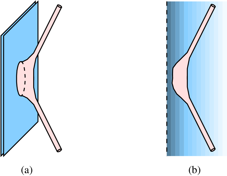
As just described, the derivation of a gauge/string duality might seem a simple algorithmic task. Of course, this is not the case and, up to now, nobody was able to apply this program to QCD, with the exception of the 2–dimensional case [15]. Nevertheless, there has been important progress in understanding with more detail some of the steps involved. In particular, how to write gauge theory Feynman diagrams as integrals over the moduli space of Riemann surfaces [16]. However, so far these direct approaches starting directly from the gauge theory side of the duality have not been very successful (see [17, 18, 19, 20, 21, 22] for interesting attempts in this direction).
Presently, there are a few inspiring models of lower dimensional gauge theories where the program can be made rigorous: the duality between 3–dimensional Chern–Simons theory and the A–model topological closed string theory on the resolved conifold [23]; and the duality between double–scaled matrix models and minimal closed bosonic string theories [24]. Usually, the string theories involved in these toy models are, in some sense, topological so that the open string theories are precisely equivalent to gauge theories. In contrast, the celebrated AdS/CFT correspondence [1, 25, 26] was obtained as the low energy limit of an underlying open/closed duality.
1.4 AdS/CFT Correspondence
Let us now briefly describe the reasoning that lead to the prototypical example of AdS/CFT correspondence. The basic idea is to apply the picture in figure 1.8 to the system of coincident D3–branes of type IIB string theory placed in 10–dimensional Minkowski space and then focus on its low energy dynamics. More precisely, we shall consider the limit of vanishing string length, , keeping the string coupling , the number of branes and the energy fixed. On one hand, the system of figure 1.8(a) has closed and open string degrees of freedom, describing bulk and brane excitations, respectively. As , all massive string modes disappear and we are left with two decoupled systems: free gravity in and supersymmetric Yang--Mills theory 55 5 In this discussion we neglect the decoupled factor associated to the freedom to move the center–of–mass of the brane system. in the 4–dimensional brane worldvolume. The Yang–Mills coupling constant is related to the string coupling by , in agreement with the generic expectations of ’t Hooft’s expansion. On the other hand, the equivalent description of figure 1.8(b) corresponds to a closed string background which is asymptotically , but is deformed by the D3--branes tension and charge. In the supergravity approximation, this is given by the metric 66 6 The solution has also non-vanishing RR 5–form but this is not important for the argument.
| (1.4) |
where is the metric on the 5–sphere, the corresponds to the branes worldvolume and
The low energy limit is slightly more subtle in this description. The limit naively applied to the closed string background (1.4) yields just free gravity in . However, this is not the full result. The vanishing of the metric time component at the location of the original branes () means that low–energy fluctuations from the point of view of an observer at infinity can be very energetic local excitations in the near horizon region . This is just the usual red–shift phenomena associated with black hole horizons. To appropriately determine the low energy limit of the near horizon region, we introduce a new coordinate which we keep fixed as . Then the near horizon geometry becomes
| (1.5) |
corresponding to the product space AdS both with radius . We conclude that the low energy limit of the dual closed string description of the brane+bulk system yields again two decoupled systems: type IIB closed strings in AdS and, as before, free gravity in . This naturally leads to the fascinating conjectured duality between 4–dimensional supersymmetric Yang–Mills (SYM) theory and type IIB string theory in AdS.
It is interesting to see that this duality follows precisely the pattern suggested by ’t Hooft’s expansion. Indeed, the ’t Hooft coupling of the gauge theory determines the worldsheet coupling constant,
controlling string effects. Clearly, the closed string worldsheet theory is weakly coupled when the dual gauge theory is strongly coupled. This is a generic feature of gauge/string dualities that makes them so powerful, but also so hard to prove. When the radius of AdS is much larger than the string length we can, in first approximation, analyze the dynamics of the low energy gravitational theory for string massless modes. Compactifying on the 5–sphere, we obtain a gravitational theory on AdS5 whose Newton constant , in units of the AdS radius, is
Therefore, the expansion of the gauge theory correspond to the perturbative treatment of gravitational interactions between string massless modes.
By now, there is a plethora of examples of the AdS/CFT correspondence. These are usually obtained by applying similar reasoning to other brane configurations in string theory. The known examples have an impressive variety, differing in spacetime dimensionality, gauge symmetry, global symmetry (like the amount of supersymmetry), particle content (including fundamental fermions), –function (including confining theories), etc. However, the crucial closed string theory dual to physical QCD remains unknown.
The use of the AdS/CFT correspondence as a tool to describe gauge theory phenomena is limited by our poor understanding of String Theory. Usually, one is restricted to the large and large regime, where the string theory reduces to a classical gravitational theory. In the past years, a great effort has been made to understand the planar limit at generic values of ’t Hooft coupling . This amounts to the full comprehension of the string worldsheet theory, including the strong coupling regime. The study of the extrapolation between large , where string theory is under control, and small , where gauge theory perturbative computations are reliable, has led to many interesting developments and ideas. From these, the most prominent is perhaps the surprising hypothesis of integrability of planar SYM [27, 28, 29, 30, 31, 32, 33, 34].
1.5 Outline of the Thesis
In this thesis we shall concentrate on effects, keeping the ’t Hooft coupling large. As explained above, this regime is dual to perturbative quantum gravity in AdS. Unfortunately, the loop expansion in the gravitational coupling is plagued with the usual ultra–violet (UV) divergences present also in flat space when the regulator length is neglected. Indeed, in most circumstances, we are forced to restrict our attention to tree level gravitational interactions, which, in AdS, are already very complex. Our strategy to go beyond tree level will be to focus on a specific kinematical limit of AdS scattering amplitudes. It is well known that, in flat space, the quantum effects of various types of interactions can be reliably re–summed to all orders in the relevant coupling constant, in specific kinematical regimes [35, 36, 37, 38, 39, 40, 41, 42]. In particular, the amplitude for the scattering of two particles can be approximately computed in the eikonal limit of small momentum transfer compared to the center–of–mass energy. In this limit, even the gravitational interaction can be approximately evaluated to all orders in , and the usual perturbative UV problems are rendered harmless by the resummation process. Moreover, at large energies, the gravitational interaction dominates all other interactions, quite independently of the underlying theory [37].
The main result of this thesis is the generalization of the eikonal approximation to high energy scattering in AdS and its interpretation from the point of view of the dual CFT. We remark that, although our results will include all terms of the expansion, there are still finite effects that are not captured by our computations. This is the case of instanton effects which give rise to the usual non–perturbative factor . Therefore we shall always consider , corresponding to small string coupling , therefore ensuring the smallness of non–perturbative effects.
As usual in investigations of the AdS/CFT correspondence, this thesis is naturally divided in two main parts: chapter 2 is mainly devoted to computations in Anti–de Sitter spacetime; while chapters 3 and 4 concern the study of the dual CFT.
We start chapter 2 by reviewing the eikonal approximation for potential scattering in Quantum Mechanics. We then rederive the standard eikonal approximation to ladder and cross ladder diagrams in flat space [35, 36], using Feynman rules in position space. This derivation makes the physical meaning of the eikonal approximation transparent. Each particle follows a null geodesic corresponding to its classical trajectory, insensitive to the presence of the other. The leading effect of the interaction, at large energy, is then just a phase determined by the tree level interaction between the null geodesics and of the incoming particles,
| (1.6) |
where is the coupling and is the propagator for the exchanged spin particle contracted with the external momenta. We shall see in section 2.28 that this intuitive description generalizes to AdS, therefore resumming ladder and cross ladder Witten diagrams. Moreover, we are able to formulate the eikonal approximation for high energy scattering in a general spacetime, emphasizing its essential properties. Closing chapter 2, we present an alternative derivation of the eikonal approximation in AdS, based on gravitational shock waves.
In chapter 3, we prepare the path for the CFT interpretation of the eikonal approximation in AdS. Firstly, we review the conformal partial wave decomposition of the CFT four point correlator
| (1.7) |
of primary operators and . In particular, we establish the S–channel () partial wave expansion of the disconnected graph
as an exchange of an infinite tower of primary composite operators of increasing dimension and spin. Secondly, we introduce an impact parameter representation for the conformal partial waves appropriate to describe the eikonal kinematical regime.
In chapter 4, we explore the consequences of the eikonal approximation in AdS for the CFT four point correlator (1.7). Using the eikonal approximation in AdS, we establish the behavior of in the limit of . The relevant limit is not controlled by the standard OPE, since the eikonal kinematics is intrinsically Lorentzian. Nonetheless, the amplitude is related to the usual Euclidean correlator by analytic continuation and can be easily expressed in terms of the impact parameter representation introduced in chapter 3.

In the eikonal regime, the S–channel partial wave decomposition of the amplitude is dominated, as in flat space, by composite states of the two incoming particles. These are dual to the composite primary operators of classical dimension and spin , already present at zero order. We then find that the eikonal approximation to controls the anomalous dimension of these intermediate two–particle states, in the limit of large and .
Heuristically, the basic idea can be summarized in two steps. Firstly, the two incoming particles approximately follow two null geodesics in AdSd+1 with total energy and relative angular momentum , as described by Figure 1.9. The corresponding –dimensional impact parameter space is the transverse hyperboloid and the minimal geodesic distance between the null geodesics is given by
Then, the eikonal approximation determines the phase due to the exchange of a particle of spin and dimension in AdS. As described above, this phase shift is determined by the interaction between the two null geodesics. We shall see that computing (1.6) in AdS gives
| (1.8) |
where is the coupling in AdS and is the Euclidean scalar propagator of dimension in the transverse space . Secondly, the phase shift is related to the anomalous dimension by the following argument. Recall that [43], due to the conformal structure of AdS, wave functions have discrete allowed frequencies. More precisely, a state of dimension with only positive frequencies will be almost periodic in global time , acquiring only a phase as . Since the interaction between the two particles occurs in a global time span of , we conclude that the full dimension of the composite state is .
We end chapter 4 focusing on the tree level contribution for the eikonal amplitude, to study the T–channel () partial wave expansion of an AdS tree level exchange graph in the same channel. We establish that a spin AdS exchange has a partial wave expansion of bounded spin and that the eikonal approximation fixes the coefficients of the intermediate primaries of highest spin . Armed with this result, we deduce that the leading contribution to , for , is determined completely by the tree level T–channel exchange, so that (1.8) is exact to all orders in the coupling . Moreover, in gravitational theories, the leading contribution to comes from the graviton [37], with and . The result (1.8) is then valid to all orders in the gravitational coupling . This provides a powerful prediction for the duality between strings on AdS and four dimensional SYM: the anomalous dimension of the above double trace operators is
| (1.9) |
for , so that the impact parameter is much larger than the radius and the effects of massive KK modes are negligible.
Finally, we present our conclusions and comments on open questions in chapter 5.
1.6 Preliminaries & Notation
This section contains the indispensable information on AdS/CFT necessary for the considerations in the subsequent chapters. We shall avoid the use of specific realizations of the AdS/CFT correspondence by considering a generic formulation summarizing its essential properties. We emphasize the importance of this section given that it introduces the powerful and infrequent notation based on the embedding of AdS space into flat space, which will be extensively used in this thesis.
1.6.1 AdS Geometry
We start by recalling that AdSd+1 space (of dimension ) can be defined as a pseudo–sphere in the embedding space . More precisely, AdS space of radius is given by the set of points
| (1.10) |
Throughout this thesis, within the context of AdS/CFT, all points, vectors and scalar products are taken in the embedding space . Also, from now on we choose units such that . It is clear from the above definition that the AdS isometry group is the Lorentz group . Rigorously, AdSd+1 is the universal covering space of the pseudo–sphere (1.10), obtained by decompactifying along the non–contractible timelike cycle associated with the action of .
We shall define the holographic boundary of AdSd+1 as the set of outward null rays from the origin of the embedding space , i.e. a point in the boundary of AdS is given by
| (1.11) |
Again, the boundary is the universal covering space of (1.11). In figure 1.10 the embedding of the AdS geometry is represented for the AdS2 case.

Usually, the AdS boundary is identified with a specific section of the light cone in , containing one representative point for each null ray. Then, the embedding space naturally induces a metric on . The metrics on two different light cone sections, and , are related by a Weyl transformation, since any can be rescaled to , yielding
Furthermore, the natural action of the Lorentz group on the space of null rays defines the action of the conformal group on 77 7 This was explained long ago by Dirac [44].. However, Lorentz transformations preserve the light cone but not the section . Thus, their action on a point needs to be compensated with an appropriate re–scaling , so that the final point belongs to . This makes the action of the conformal group less transparent. Therefore, in this thesis, we shall use the coordinate–invariant definition (1.11) of the AdS boundary. Nevertheless, to develop some intuition on this invariant language, and to make contact with other studies on AdS/CFT, we shall now briefly review the two most common choices of light cone sections or, equivalently, representations of the AdS boundary.
The first choice of light cone section is associated with the familiar statement that the boundary of AdSd+1 is –dimensional Minkowski space. In this case, is defined by the set of points satisfying
| (1.12) |
with a fixed null vector in . This choice is usually associated with AdS written in Poincaré coordinates. These are obtained by splitting the embedding space as the direct product , with the containing the null vector . Poincaré coordinates , where , , are then defined by
| (1.13) |
with the null vector in satisfying . In this expression, and often in the rest of the thesis, the point represents a point in the embedding space at the origin of the factor. In other words, parametrizes the subspace of orthogonal to and . It is now trivial to compute the AdS metric in Poincaré coordinates,
Similarly, one can parametrize the section using , by writing
| (1.14) |
Then, the induced metric on is indeed the Minkowski one. The fact that as leads to the usual statement that the AdS boundary is at . In figure 1.11(a) we plot this choice of section for the AdS2 case.

The coordinate system (1.13) only covers part of AdS and, similarly, the section is not the entire AdS boundary. To see this, we use the boundary point to divide AdS in an infinite sequence of Poincaré patches, separated by the null surfaces and labeled by integers increasing as we move forward in global time. The Poincaré coordinates (1.13) cover only the patch, which is the one spacelike related to the boundary point , as shown in figure 1.12.

The splitting of the embedding space establishes a direct map between the usual generators of the conformal group acting on and the Lorentz generators of ,
with the indices varying over all directions and with the indices restricted to the factor. Notice that conformal transformations that leave the –dimensional metric invariant (the Poincaré group) are, in this language, the transformations that preserve the section . Indeed, acting on , as defined in (1.14), we obtain
where . In contrast, the transformations that do not preserve the section , sending to , induce a conformal scaling of the –dimensional metric
Dilatations,
and special conformal transformations,
belong to this class.
The other frequent face of the AdS boundary is , with representing the time direction. This is usually associated with AdS written in global coordinates. Here, one splits the embedding space as the product of a timelike by an Euclidean . It is convenient to define the timelike plane as the space spanned by two orthogonal and normalized timelike vectors in , that is two points in AdSd+1 satisfying . One can then introduce global coordinates for AdS as follows
| (1.15) |
where the decompactified angle is the global time, is a radial coordinate and the vector parametrizes the unit sphere orthogonal to and . A natural choice of light cone section is the set of null vectors in with unit projection onto the chosen timelike plane, i.e. the set of points
| (1.16) |
This corresponds to the intuitive idea that one approaches the AdS boundary as . Indeed, as . In figure 1.11(b) we plot this choice of light cone section for the AdS2 case. Finally, we point out that one must be cautious when working in embedding coordinates since two general bulk points and , or two boundary points and , related by a global time translation of integer multiples of , have the same embedding in .
In the sequel, we will find the transverse hyperbolic space , given by the upper mass–shell
where is future directed. We shall denote with the future Milne wedge given by , with future directed. Similarly, we shall use and to designate the past Milne wedge and the associated transverse hyperbolic space. Finally, we represent by
a generic integral on AdSd+1 and , respectively. With this notation, we have
where and .
1.6.2 AdS Dynamics
Particle propagation simplifies considerably in the embedding space language. For example, the timelike geodesic corresponding to a particle stopped at in global coordinates (1.15), is simply the intersection, in the embedding space , of the timelike plane generated by and , with the pseudo–sphere defining AdS. Then, by Lorentz transformations, we conclude that any timelike geodesic is given by the intersection of a timelike plane through the origin of with the pseudo–sphere defining AdS. Moreover, the energy of this particle, as measured by an observer following another timelike geodesic, is just a measure of the intersection angle between the two timelike planes defining the geodesics. Most importantly for our purposes are null geodesics in AdS. These are also geodesics in the embedding space ,
with , and . As it is well known, lightlike geodesics reach the AdS boundary in finite global time. More precisely, the above null geodesic starts at the point of the AdS boundary, travels during a global time interval , and ends up again in the AdS boundary at the point . On the other hand, if one tries to reach a null geodesic by taking the limit of a timelike geodesic with infinite energy, one obtains an infinite sequence of null geodesics bouncing back and forth on the AdS boundary between consecutive images of and .
The embedding space is also very useful to describe field dynamics in AdS. The d’Alembertian operator in AdS can be written using just partial derivatives in the flat embedding space,
| (1.17) |
Rigorously, in order to take partial derivatives , it would be necessary to extend the domain of the fields from AdS to the full embedding space. However, the action of is independent of this extension so that we can use this convenient notation without reference to any extension of the domain. On the other hand, this shows that a scalar field satisfying the massless Klein–Gordon equation in the embedding space,
and the scaling relation
obeys the massive Klein–Gordon equation in AdS,
with
The wave equation in AdS requires the specification of boundary conditions on the AdS timelike boundary. Firstly, one needs to determine the behavior near the AdS boundary of solutions of the Klein–Gordon equation in AdS. For this purpose, it is convenient to introduce generic coordinates for AdS, related with a given light cone section parametrized by ,
| (1.18) |
where is the inverse of the radial coordinate along the light cone so that corresponds to the boundary at infinity. The null vectors satisfy . Notice that the Poincaré coordinates (1.13) are precisely of this form with given in (1.14) and a fixed null vector. Similarly, the AdS global coordinates (1.15) also have the generic form (1.18) with playing the role of , the boundary coordinates and
In the coordinate system (1.18) the AdS metric near the boundary reads
Therefore, a solution of the massive Klein–Gordon equation in AdS can have two leading behaviors as ,
| (1.19) |
where we have normalized for later convenience. This asymptotic behavior is crucial for the AdS/CFT correspondence.
The Feynman propagator in AdS satisfies
As usual in quantum field theory, the Lorentzian propagators require an appropriate prescription as crosses the light cone of . The best way to accomplish this is to define the Lorentzian propagator by a Wick rotation of the Euclidean one. The latter satisfies the similar equation
but now on the hyperbolic space , which is the Euclidean version of AdSd+1. The propagator can be explicitly written using the hypergeometric function,
| (1.20) |
where
is a normalization constant and
is the Lorentz invariant chordal distance, which is always positive in the Euclidean regime. In contrast, in the Lorentzian regime there are negative (timelike) chordal distances which require a prescription to pass through the branch points of at and . The correct prescription is obtained by following the complex path of as the AdS points are Wick rotated from the Euclidean to the Lorentzian setting.

To see the explicit result of this prescription, write in global coordinates (1.15). Choosing for simplicity, we obtain
Then, consider the standard Wick rotation parametrized by ,
| (1.21) |
with in the Euclidean setting and in the Lorentzian one. The Lorentzian propagator is then given by the function in the Riemann sheet containing the endpoint of the complex path , starting from the Euclidean point in the positive real axis. In figure 1.13, we plot the paths for several values of global time , which is sufficient since the paths in (1.21) are insensitive to the sign of . Denoting with , the region where and are spacelike separated, we have
In the region the point is spacelike separated from (see figure 1.14). In general, for
we have and therefore there is no phase factor contribution from the branch cut of the hypergeometric function in the propagator expression. Following carefully the spiral structure of the complex paths in figure 1.13, we conclude that, in these regions, the factor in the propagator yields a phase
For , the complex paths end on the branch cut of the hypergeometric function. In this case, one should use as the argument of the hypergeometric function. These comments are summarized in figure 1.14.

In the AdS/CFT correspondence, there is also a bulk to boundary propagator. This can be obtained as a limit of the bulk to bulk propagator described above. To approach the boundary, we write a point in AdS in the form (1.18) and take the limit ,
| (1.22) |
where now numbers the Poincaré patches of as in figure 1.12. We shall often use the prescription
which works for in the Poincaré patches of (see figure 1.12). As a function of AdS, the bulk to boundary propagator satisfies the Klein–Gordon equation in AdS with mass squared . Therefore, it must follow the general asymptotic behavior (1.19). Indeed, as approaches the boundary ()
| (1.23) |
where
is the boundary to boundary propagator and is the –dimensional Dirac delta function on the lightcone section . The standard normalization of the bulk to boundary propagator is chosen such that there is no factor of multiplying the delta function in (1.23). As we shall see, our normalization, obtained from the limit of the bulk to bulk propagator, is more convenient for the computation of correlation functions within the AdS/CFT correspondence [45].
Finally, we recall that the bulk to boundary propagator can be used to write a generic solution of the Klein–Gordon equation in AdS
Invariance of this integral under a change of light cone section requires the boundary wave function to be an homogeneous function on the light cone,
1.6.3 CFT on the AdS Boundary
We shall define the conformal field theory (CFT) on its natural habitat, the light cone of . A CFT correlator of scalar primary operators located at points , can then be conveniently described by an amplitude
invariant under , and therefore only a function of the invariants
The amplitude is homogeneous in each entry
where is the conformal dimension of the –th scalar primary operator. In this language, one recovers standard results on –dimensional CFT’s by choosing a specific section of the light cone of . Correlations functions of primary operators defined on different light cone sections and with , are then related by
as required for these CFT correlators. The power of this notation is that it makes symmetry properties transparent. For example, the two point function of two primary operators can only be a function of the invariant . Moreover, the homogeneity condition implies the vanishing of the two point function for operators with different conformal dimension and fixes
for operators of the same dimension. Notice that in the light cone section (1.12) we have , which gives the standard flat space CFT two point function of primary operators. In the AdS/CFT context, it is convenient to normalize CFT operators such that the two point function is given by the boundary to boundary propagator defined in the previous section,
The three point function
is also determined, up to a constant, by conformal symmetry, since
is the only possible combination of the Lorentz invariants with the required scaling properties.
In this thesis, we shall focus a great deal of our attention on four point amplitudes of scalar primary operators. More precisely, we shall consider correlators of the form
where the scalar operators and have dimensions
respectively. It is then convenient to write the four point amplitude as
| (1.24) |
so that is a generic function of the two cross–ratios and , which we define, following [46, 47], in terms of the kinematical invariants as 88 8 Throughout the thesis, we shall consider barred and unbarred variables as independent, with complex conjugation denoted by . In general when considering the analytic continuation of the CFTd to Euclidean signature. For Lorentzian signature, either or both and are real. These facts follow simply from solving the quadratic equations for and .
| (1.25) |
With this definition, the disconnected graph gives .
1.6.4 AdS/CFT Correspondence
We are now in position to state the generic conjectured correspondence between string theories in AdSd+1 and conformal gauge theories defined on the AdS boundary. Since both theories have the same symmetry group , it is not unreasonable to believe that there is a duality between them. Our point of view will be to find specific CFT properties dictated by the existence of a dual string theory on AdS. Therefore, we consider a generic gauge theory with quantum fields transforming in the adjoint representation of the gauge group 99 9 These include gauge fields or adjoint scalars. We will not consider the case of particles (like quarks) transforming in the fundamental representation since, from the general discussion of section 1.3, these are expected to be dual to open strings.. The basic gauge invariant local operators are single trace,
where is an arbitrary function (usually, a polynomial) of the fields and their derivatives. Theories with a large limit have an action functional of the form
where is, in principle, an arbitrary function of the operators , encoding the coupling constants of the theory (like the ’t Hooft coupling in Yang–Mills theory). In most cases the action is single trace and is just a linear function. Furthermore, we shall restrict our attention to conformal field theories, where the lagrangian density is an exactly marginal operator of dimension (see [48] for RG flows within AdS/CFT). The AdS/CFT correspondence states that, for each single trace primary operator of the CFT, there is a field in AdS, corresponding to a particular string mode. On the other hand, multiple trace local operators are dual to multistring states in AdS. In a given realization of the AdS/CFT correspondence, this map can usually be made very precise. Here, we restrict ourselves to generic features of the correspondence. For instance, a scalar field in AdS with mass squared , is dual to a scalar primary operator of dimension .
The CFT dynamics is defined by the correlation functions of its gauge invariant local operators. Furthermore, it is enough to consider single trace operators, since multiple trace operators can be obtained from the operator product expansion (OPE) of the first 1010 10 See [49] for the relation between multiple trace deformations and AdS boundary conditions.. The dynamical information of the AdS/CFT correspondence can then be embodied in the relation between the generating functional for CFT correlators and the string theory partition function with appropriate boundary conditions on the AdS boundary. In the case of the scalar field mentioned above, we have
| (1.26) |
where the AdS scalar field tends to the source at the AdS boundary as defined by (1.19). In the Lorentzian version of AdS/CFT, this boundary condition and the equations of motion do not uniquely determine the field in the bulk. This freedom corresponds to different choices of initial and final states for the boundary correlators [50, 51]. In this thesis, we shall always consider correlation functions in the vacuum state, by analytically continuing from the Euclidean theory. CFT correlation functions are obtained by differentiating with respect to the source . On the string theory side, each differentiation sends into AdS a closed string in the state . In other words, a CFT point function is given by the string amplitude associated to the sum over all worldsheets embedded in AdS with punctures fixed at the AdS boundary as in figure 1.15. Different CFT operators correspond to different boundary conditions on the worldsheet fields at the punctures.

When the AdS radius is much larger than the string length , the low energy gravitational approximation, describing the string massless modes, is reliable
Here, represents all massless fields in AdS. Pictorically, the infinite string tension collapses the surface in figure 1.15 to Witten diagrams describing particle exchange in AdS [25]. In the case of SYM, we have seen that this regime of small strings in AdS corresponds to large ’t Hooft coupling in the gauge theory. In general, one expects the gravitational regime of the string theory to be dual to some strongly coupled gauge theory. In addition, the perturbative expansion in the gravitational coupling corresponds to the expansion in the CFT. The Witten diagrams are drawn using the propagators and interaction vertices associated to the effective action for the string lightest modes. We shall concentrate on correlation functions of scalar primary operators. These are obtained from Witten diagrams with bulk to boundary propagators, connected to the points , glued to bulk to bulk propagators of the exchanged particles, using the interaction vertices contained in the effective action.
As a toy example, consider our scalar field with a cubic interaction in AdS,
A solution to the equation of motion , satisfying the required boundary conditions, can be obtained by iterating the following integral equation
| (1.27) |
Then, the value of the action for this classical solution is given by the diagrammatic expansion
| (1.28) |
where each Witten diagram is evaluated using the following rules: each vertex yields a factor of and is integrated over AdS; internal lines represent bulk to bulk propagators; lines connecting to the boundary represent bulk to boundary propagators; and the boundary points are integrated over with weight . The correlation functions are obtained just by taking functional derivatives of (1.28). For example, the two point function is
and the three point function is
So far we have considered the classical approximation . Quantum effects in AdS correspond to Witten diagrams with internal loops. Including these in (1.28) defines the quantum effective action, which becomes the new generating function for CFT correlators.
Chapter 2 Eikonal Approximation
Geometric optics can be obtained as the infinite frequency limit of wave propagation. In this limit, the phase function satisfies the eikonal equation
where is the refraction index of the medium. Light rays are then given by the integral curves of the gradient of the phase function. The function is also known as the lapse function. This terminology arises from the problem of finding the fastest light path from the boundary of a given compact space , with refraction index , to a point . In this case, the lapse function is the shortest time that light takes to arrive at point starting from the boundary of .
In this chapter, we shall describe the eikonal approximation for particle scattering. We start with the simpler case of potential scattering in non–relativistic quantum mechanics since all important concepts are already present in this computation. We then move to quantum field theory (QFT) on Minkowski spacetime and rederive the eikonal approximation using position space Feynman rules. With this in mind, we are able to generalize the eikonal approximation to particle scattering in AdS and other spacetimes. Finally, we use gravitational shock wave techniques to establish an alternative, perhaps more physical, derivation of the AdS eikonal approximation.
2.1 Potential Scattering in Quantum Mechanics
Consider the Schrödinger equation
governing the wave function of a non–relativistic particle scattering in the potential at very high energy . We write
so that free propagation with momentum corresponds to a linear phase
with . With this definition, the standard scattering amplitude is given by [52]
where and are the initial and final momenta, respectively, determining the scattering angle through .
In the presence of a non–vanishing potential, the phase function obeys the eikonal like equation
Then, the leading correction in is simply given by the accumulated phase shift along the free particle’s trajectory
The eikonal approximation is valid at high energies and fixed momentum transfer . In this regime, the scattering angle is very small and the momentum transfer is essentially orthogonal to the propagation direction . Finally, the eikonal scattering amplitude reads
| (2.1) |
with
Notably, the eikonal approximation resums an infinite number of terms in the Born perturbative expansion, yielding a scattering amplitude only valid in a specific kinematical regime, but including contributions of all orders in the scattering potential . Interestingly, the eikonal amplitude (2.1) satisfies the optical theorem [53]
For spherically symmetric potentials, one usually expands the scattering amplitude in partial waves
where are the Legendre polynomials and is the phase shift associated to the spin partial wave. In the eikonal regime, one considers large energy and small scattering angle, keeping their product fixed by the momentum transfer . In this limit, the sum over spin can be replaced by an integral over the impact parameter and the Legendre polynomials reduce to the zeroth order Bessel function , giving the known impact parameter representation
The eikonal amplitude (2.1) reduces exactly to the same expression after performing the angular integral in transverse space and identifying and for large . In other words, the eikonal approximation determines the leading behavior of the phase shift at large spin.
2.2 Minkowski Spacetime
In relativistic QFT, all interactions are mediated by particle exchange and there is no direct analogue of a static potential like in the previous section. Therefore, the generalization of the semi–classical eikonal approximation is not obvious. Nevertheless, this generalization was found long time ago [35, 36]. In this section we shall rederive the standard eikonal amplitude for high energy scattering in Minkowski spacetime from a position space perspective. This will prove to be useful because the physical picture here developed will generalize to scattering in AdS. We shall consider –dimensional Minkowski space in close analogy with AdSd+1. At high energies
we can neglect the masses of the external particles and, for simplicity, we shall consider first an interaction mediated by a scalar field of mass . In flat space we may choose the external particle wave functions to be plane waves , so that the amplitude is a function of the Mandelstam invariants
We then have
The eikonal approximation is valid for , where the momentum transferred is approximately orthogonal to the external momenta.
The momenta of the incoming particles naturally decompose spacetime as . Using coordinates in and in the transverse space , a generic point can be written using the exponential map
| (2.2) |
where the vector fields and are defined by
The incoming wave functions are then
The coordinate is an affine parameter along the null geodesics describing the classical trajectories of particle 1. This set of null geodesics, labeled by and , is then the unique congruence associated with particle 1 trajectories. Since is a Killing vector field, these geodesics have a conserved charge . At the level of the wave function this charge translates into the condition
Notice also that the wave function is constant along each geodesic of the null congruence,
where is the momentum vector field associated to particle 1 trajectories. Hence
Finally, the field equations imply that is independent of the transverse space coordinate . Similar comments apply to particle 2.
Neglecting terms of order , the outgoing wave functions for particles 1 and 2 are still independent of the corresponding affine parameter, but depend on the transverse coordinate ,
The dependence in transverse space is determined by the transferred momentum . Physically, the transverse space is the impact parameter space. In fact, for two null geodesics associated to the external particles 1 and 2, labeled respectively by and , the classical impact parameter is given by the distance .

The exchange of scalar particles described by figure 2.1 gives the following contribution to the scattering amplitude
where is the spacetime volume, is the coupling and where and are, respectively, the massless and massive Feynman propagators satisfying
The basic idea of the eikonal approximation is to put the horizontal propagators in figure 2.1 almost on–shell. This is usually done in momentum space. For example, for the propagator between vertices and , we approximate
where is the total momentum transferred up to the vertex at . The physical meaning of this approximation becomes clear in the coordinates (2.2),
| (2.3) | |||||
In words, particle 1 can propagate from to only if lies on the future directed null geodesic that starts at and has tangent vector . This intuitive result can be derived directly in position space. In fact, in coordinates (2.2), the propagator satisfies
Since for particle 1 we have , for high energies and (2.3) follows.
The eikonal approximation to the position space propagators greatly simplifies the scattering amplitude for the exchange of scalar particles
with
Furthermore, the sum over permutations can be used to extend the integrals over the affine parameters of external particle trajectories to the full real line,
where
Summing over , one obtains (the term corresponds to the disconnected graph)
| (2.4) |
The integral can be interpreted as the interaction between two null geodesics of momentum and describing the classical trajectories of the incoming particles. In fact, using as integration variables the natural affine parameters along the geodesics, one has
Since the integral only depends on the impact parameter of the null geodesics, equation (2.4) simplifies to
| (2.5) |
Explicit computation yields the Euclidean propagator of mass in the transverse space
and we recover the well known eikonal amplitude.
The generalization of the above method to interactions mediated by a spin particle is now straightforward. We only need to change the integral describing the scalar interaction between null geodesics. The spin exchange alters the vertices of the local interaction, as well as the propagator of the exchanged particles. In general, the vertex includes momentum factors with a complicated index structure. However, in the eikonal regime, the momenta entering the vertices are approximately the incoming momenta . Therefore, the phase should be replaced by 11 1 The sign indicates that, for odd , particles 1 and 2 have opposite charge with respect to the spin interaction field. With this convention the interaction is attractive, independently of .
where is the propagator of the massive spin field. Recall that the equations of motion for a spin field imply that is symmetric, traceless and transverse (), together with the mass–shell condition . Therefore, the relevant part of the propagator at high energies is given by
where the indices and are separately symmetrized with weight and is the scalar propagator of mass . The neglected terms in are trace terms, which vanish since , and derivative terms acting on , which vanish after integration along the two interacting geodesics. Compared to the scalar case, we have then an extra factor of , so that
Note that we have normalized the coupling so that the leading behavior of the tree level amplitude at large is given by . In the particular case of we have , where is the canonically normalized Newton constant.
It is known [54, 55] that the eikonal approximation is problematic for exchanges. In this case, the large incoming momentum can be exchanged by the mediating particle, interchanging the role of in intermediate parts of the graph. The eikonal approximation estimates correctly the large behavior of the amplitude at each order in perturbation theory, but underestimates the relative coefficients, which do not resum to an exponential. Nonetheless, this is not problematic, since exactly in the case the higher order terms are suppressed by powers of . For the problematic hard exchanges are suppressed at large energies and the eikonal approximation is valid. On the other hand, for the QED case where , there is a different set of graphs involving virtual fermions [56, 55] that dominate the eikonal soft photons exchange. Therefore, also for , the validity of the eikonal approximation is in question. None of these problems arise, though, for the most relevant case, the gravitational interaction with .
2.2.1 Partial Wave Expansion
As in non-relativistic quantum mechanics, the Lorentz invariant scattering amplitude can be conveniently decomposed in S–channel partial waves
| (2.6) |
with
related to the scattering angle and with the phase shift for the spin partial wave 22 2 We choose a non standard normalization and notation for the phase shifts for later convenience. To revert to standard conventions, one must replace by .. The angular functions are eigenfunctions of the Laplacian on the sphere at infinity, with eigenvalue , and are polynomials in of order , whose explicit form depends on the dimension of spacetime. They can be written as hypergeometric functions
and they are normalized so that corresponds to free propagation with no interactions. Unitarity then implies . The amplitude itself can be computed in perturbation theory
where corresponds to graph (a) in figure 2.2 describing free propagation in spacetime. All S–channel partial waves contribute to with equal weight one, and vanishing phase shift.

In the eikonal regime we are interested in the limit of small scattering angle. If the amplitude diverges at , then its partial wave expansion contains partial waves with unbounded intermediate spin . In fact, one may then replace the sum over with an integral over the impact parameter ,
denoting the phase shift by from now on. More precisely, if we consider the double limit
| (2.7) |
the angular functions become, in this limit, Bessel functions defining the impact parameter partial waves ,
| (2.8) |
with . The impact parameter limit corresponds to approximating the sphere at infinity by a transverse Euclidean plane . This limit takes the sphere harmonic functions into the plane harmonic functions . Returning to (2.6) and replacing the sum over spins by the integral over the impact parameter , one obtains the impact parameter representation of the amplitude
| (2.9) |
where . Comparing with (2.5), we find that the leading behavior of for large , which controls small angle scattering, is given by the tree–level interaction between two null geodesics,
Indeed, a simple way of stating the eikonal approximation is to say that the leading behavior of the phase shift for large , is dominated by the leading tree–level amplitude and it is therefore determined by a simple Fourier transform,
| (2.10) |
Moreover, the dominant interaction in comes from T–channel exchanges of spin massless particles, so that the full amplitude (2.9) approximately resums the crossed–ladder graphs in figure 2.2(b). In the limit of high energy , the mediating particle with maximal dominates the interaction. In theories of gravity, this particle is the graviton, with [37].
To understand in more detail the generic behavior of amplitudes for small scattering angle and large energies, consider some sample interactions shown in figure 2.3 contributing to , where the exchanged particle is massless and has spin .

The contribution of graph 2.3(a) to has the generic form
| (2.11) |
The polynomial part in contributes to partial waves with spin . This can also be understood in the impact parameter representation (2.10), since polynomial terms in give, after Fourier transform, delta–function contributions to the phase shift localized at . The universal term contributes, on the other hand, to partial waves of all spins and gives a phase shift at large given by
| (2.12) |
where is the scalar massless Euclidean propagator in transverse space . At high energies, the maximal dominates. Graph 2.3(b) is obtained by interchanging the role of and in (2.11) , and therefore is proportional to . The corresponding intermediate partial waves have spin . Finally, graph 2.3(c) is obtained from 2.3(a) by replacing by and therefore by sending . Using the fact that , we can again expand the U–channel exchange graph 2.3(c) in the form where are the phase shifts of the T–channel exchange, whose large spin behavior is given by (2.12). At large spins, the contribution to the various partial waves is alternating in sign and averages to a sub–leading contribution. Finally, the contact graph 2.3(d) only contains a spin zero contribution. We conclude that, at large spins and energies, the T–channel exchange of a graviton in graph 2.3(a) dominates all other interactions.
2.3 Anti–de Sitter Spacetime
Let us now follow the intuitive picture developed in the previous section to generalize the eikonal approximation to hard scattering in Anti–de Sitter spacetime [57]. In this section we derive an eikonal approximation in AdS summing ladder and cross ladder Witten diagrams. The corresponding partial wave analysis is postponed to the next chapters. As explained in section 1.6.1, we define AdSd+1 space, of dimension , as the pseudo–sphere (1.10) of radius embedded in . Then, we denote a point AdS by a point in the embedding space obeying .
Consider the Feynman graph in figure 2.1, but now in AdS. For simplicity, we consider the exchange of an AdS scalar field of dimension and, for external fields, we consider scalars of dimension and . Then, the graph in figure 2.1 evaluates to
| (2.13) |
where stands for the scalar propagator of mass in AdS, satisfying
| (2.14) |
In general, this amplitude is very hard to compute. However, we expect some drastic simplifications for specific external wave functions describing highly energetic particles scattering at fixed impact parameters. In analogy with flat space, we expect the eikonal approximation to correspond to the collapse of the propagators and into null geodesics approximating classical trajectories of highly energetic particles.
2.3.1 Null Congruences in AdS and Wave Functions
As mentioned in section 1.6.2, a null geodesic in AdS is also a null geodesic in the embedding space
where and the tangent vector satisfies
We will follow the intuitive idea that the wave functions and correspond to the initial states of highly energetic particles moving along two intersecting congruences of null geodesics. As described in the previous section, in flat space there is a one–to–one correspondence between null momenta (up to scaling) and congruences of null geodesics. On the other hand, in AdS the situation is more complicated. Given a null vector there is a natural set of null geodesics passing through all points belonging to the hypersurface , as shown in figure 2.4(a). However, to construct a congruence of null geodesics we need to extend this set to the full AdS space. Contrary to flat space, in AdS this extension is not unique because the spacetime conformal boundary is timelike. We will now describe how to construct such a congruence in analogy with the construction presented for flat space.

We start with two null vectors associated with the incoming particles, as represented in figure 2.4(b) and normalized as in flat space
The transverse space is naturally defined as the intersection of the two null hypersurfaces associated to and . It is the hyperboloid defined by
In order to introduce coordinates in AdSd+1 in analogy with (2.2), we choose an arbitrary reference point in this transverse space . This allows us to define the vector fields
which, from the embedding space perspective, are respectively the generators of parabolic Lorentz transformations in the and –plane. They therefore generate AdS isometries. We may now introduce coordinates for AdSd+1 as follows
| (2.15) |
where . It is important to realize that, contrary to the flat space case, and therefore the order of the exponential maps in (2.15) is important, as will become clear below.
As for flat space, the coordinate is an affine parameter along null geodesics labeled by and , which form the desired congruence for particle 1. In fact, (2.15) can be written as
Hence, the geodesics in the null congruence associated to particle 1 are given by
| (2.16) |
where
The normalization of the momentum and affine parameter of the classical trajectories is fixed by demanding, as in flat space, that the conserved charge . This gives
Let us remark that different choices of give different congruences, all containing the null geodesics , which lay on the hypersurface at . Starting from this hypersurface, we then constructed a congruence of null geodesics using the AdS isometry generated by .

Contrary to flat space, the curves defined by constant and in the coordinate system (2.15) are not null geodesics (except for the curves on the surface which are null geodesics with affine parameter ). These curves are the integral curves of the Killing vector field . In fact, these curves are not even null, as can be seen from the form of the AdS metric in these coordinates
| (2.17) |
where is the metric on the hyperboloid . To construct the null congruence for particle 2, we introduce new coordinates for AdSd+1 as follows
| (2.18) |
The two sets of coordinates are related by
| (2.19) |
The congruence associated with particle 2 is then the set of null geodesics
| (2.20) |
with
so that the conserved charge . In figure 2.5 we plot the curves of constant and (left) and of constant and (right) in the simplest case of AdS2.
As in flat space, the wave function describing particle 1 carries energy
Therefore we choose
where the function is approximately constant over the length scale , more precisely . The Klein–Gordon equation for the wave function implies
since, as in flat space, the coordinate satisfies
The above equation can then be solved expanding in powers of ,
Since the eikonal approximation gives only the leading behavior of the scattering amplitude at large , it is enough to consider only the first term so that, to this order, we have
as expected. We conclude that the function is a smooth transverse modulation independent of the affine parameter of the null geodesics associated with the classical trajectories of particle 1. Similar reasoning applied to particle 2 leads to
Finally, since in the eikonal regime the particles are only slightly deviated by the scattering process, to leading order in the outgoing wave functions are also independent of the corresponding affine parameters,
with the same requirement .
We have kept the discussion of this section completely coordinate independent. On the other hand, given the choice of and , the embedding space naturally splits into , with spanned by and and with its orthogonal complement. Then, the points , and are timelike points in , with the transverse space the upper unit mass–shell on . Finally, it is natural to introduce Poincaré coordinates similar to (1.13),
where parametrizes the orthogonal to and and is a radial coordinate. As explained in section 1.6.1, in these coordinates, the action of leaves the radial coordinate fixed and induces translations in ,
along the time direction indicated by . Similar remarks apply to with the roles of and interchanged.
2.3.2 Eikonal Amplitude
We are now in position to compute the leading behavior of the amplitude (2.13) for the exchange of scalars in AdS at large , using the techniques explained in section 2.2. The first step is to obtain an approximation for the AdS propagator similar to (2.3). Since for particle 1 we have , we can approximate
in equation (2.14) for the propagator of particle 1 between vertices and , obtaining
The solution,
| (2.21) |
has the natural interpretation of propagation only along the particle classical trajectory and, in these coordinates, takes almost exactly the same form as the corresponding propagator (2.3) in flat space. With this approximation to the propagator, the amplitude (2.13) associated with the exchange of scalar particles simplifies to
where
Notice that the extra powers of and come from the integration measure in the and coordinates, respectively. As for flat space, the integrals over the affine parameters can be extended to the real line so that, after summing over , we obtain
| (2.22) |
with
This can be rewritten as the tree–level interaction between two classical trajectories of the incoming particles described by (2.16) and (2.20), which are labeled respectively by and ,
Hence, the AdS eikonal amplitude just obtained is the direct analogue of the corresponding flat space amplitude (2.4). The eikonal interaction is depicted in figure 2.6.

The generalization of the above result to the case of interactions mediated by a minimally coupled particle of spin is straightforward, and we shall only give the relevant results. At high energies, the only change concerns the propagator , which now should be replaced by the propagator of the spin– particle contracted with the null momenta of the geodesics
where the indices are tangent indices to AdS. This follows immediately from the fact that, at high energies, covariant derivatives in interaction vertices can be replaced by and for particle one and two, respectively. The spin– propagator is totally symmetric and traceless in the indices (and similarly in the indices ), it is divergenceless and satisfies
| (2.23) |
where the indices and are separately symmetrized, and where the terms in contain derivatives of and are not going to be of relevance to the discussion which follows, since they give subleading contributions at high energies. The eikonal expression (2.22) is then valid in general, with the phase factor now replaced by
| (2.24) |
Note that we have normalized the interaction coupling as in flat space, where the tree level amplitude is given by at large .
Finally, we remark that the explicit expression (2.24) for the phase shift in (2.22) is not valid for generic values of the impact parameter [58]. In the gravitational case, we expect the semi–classical eikonal approximation to breakdown when the the impact parameter is smaller than (or of the order of) the Schwarschild radius . In fact, the regime of black hole formation in AdS has been related to the saturation of the Froissart bound in the dual gauge theory [59, 60, 61, 62]. Furthermore, in string theories, string effects become relevant at small impact parameters, when the tidal forces produced by one string are strong enough to change the internal state of the other. We shall return to this issues with more detail in the concluding chapter.
2.3.3 Transverse Propagator
Now we compute the integral . Its last expression shows that it is a Lorentz invariant local function of and . Moreover, it is invariant under
and it scales like when and . Therefore, the integral is fixed up to an undetermined function ,
with defined in analogy with flat space
| (2.25) |
To determine the function we use equation (2.23), contracting both sides with
and integrating against
Here we discuss the simplest case of , leaving for clearness of exposition the general case to appendix 2.A. Consider then first the integral of the RHS of (2.14). Using the explicit form of the –function in the coordinate system,
we obtain
| (2.26) |
Next we consider the LHS of (2.14). Explicitly parametrizing the metric on in (2.17) as
| (2.27) |
where , we have that
We do not show the explicit terms of the form since they will vanish once integrated along the two geodesics. Integrating in we conclude that (2.26) must be equated to
Using the fact that
we finally deduce that
In appendix 2.A we show that this last equation is also valid for general spin . We conclude that the function is the scalar Euclidean propagator in the hyperboloid of mass squared and corresponding dimension . Denoting this propagator by , the eikonal amplitude can be written as
| (2.28) |
with given by (2.25). In the particular case of gravitational interactions in AdS5, the same result was recently derived in [63], using different approaches.

2.3.4 Localized Wave Functions
The eikonal amplitude in AdS has a striking similarity with the standard flat space eikonal amplitude. However, an important difference is the factor in the definition (2.25) of , which makes the exponent in the eikonal amplitude (2.28) divergent for and . This divergence can be traced back to the collinearity of the tangent vectors and of the null geodesics labeled by and describing classical trajectories of particle 1 and 2, respectively. When , one null geodesic can be seen as the reflection of the other on the AdS boundary (see figure 2.7). Thus, the propagator from a point on one geodesic to a point in the other diverges, since these points are connected by a null geodesic. This is the physical meaning of the divergence at . Clearly, we should doubt the accuracy of the eikonal approximation in this case of very strong interference. To avoid this annoying divergence, from now on we shall localize the external wave functions of particle 1 and 2 around and , respectively. More precisely, we shall choose
| (2.29) |
where the profile is localized in the region and it is normalized as
| (2.30) |
On the other hand, the smoothness condition requires . The two conditions,
are compatible for high energy scattering, when the de Broglie wavelength of the external particles is much shorter than the radius of AdS (). With this choice of external wave functions, the amplitude simplifies to
| (2.31) |
where now
| (2.32) |
The eikonal amplitude (2.31) is the main result of this chapter which will be explored in great detail in chapter 4. In the remainder of this chapter we shall extend the eikonal approximation to high energy scattering in general spacetimes and rederive the amplitude (2.31) using gravitational shock waves.
2.4 General Spacetime
The position space derivation of the eikonal amplitude for flat and AdS spacetimes share many features that suggest a more general description valid for generic backgrounds. This section is an attempt to achieve such synthesis. As in the previous sections, we consider scattering of scalar particles. We also neglect their masses since they are irrelevant in the eikonal regime.
The starting point is the identification of eikonal wave functions and their associated congruences of null geodesics describing highly energetic external particles. These wave functions have the form
where the phase function obeys
| (2.33) |
The first condition comes from the leading term at large in the Klein–Gordon equation . The second is less obvious but it will be needed in the derivation of the eikonal approximation. With these two conditions, any function of satisfies the massless Klein–Gordon equation. The semi–classical wave function describes highly energetic particles following null geodesics with tangent vector
Indeed, the condition implies that the null vector field obeys the geodesic equation
Particle’s trajectories are then given by the exponential map
Furthermore, the Klein–Gordon equation at leading order in , imposes the transversality
of the modulation function .
In the computation of the eikonal amplitude it is convenient to use a coordinate system built from the phase function , the affine parameter of the null geodesics and some other transverse coordinates . In this coordinate system we have
| (2.34) |
In addition, the condition is equivalent to the closure of the Hodge dual of the the 1–form . Writing the volume form as
we have
and the condition reduces to
| (2.35) |
The results (2.34) and (2.35) are sufficient to obtain an eikonal approximation for the propagators of the external particles, similar to (2.3) and (2.21). At leading order in , one can replace in the equation
obtaining
and hence,
| (2.36) |
This is the essential mark of the eikonal regime: propagation is non–zero only along the classical free trajectories of the external particles.
The general eikonal amplitude can now be derived just by following the same steps as for Minkowski and AdS spacetimes. The scattering process in the eikonal kinematics is characterized by the external wave functions
As before, we start from the graph in figure 2.1 describing the exchange of scalar particles of mass ,
Using coordinates for and for , one can use the eikonal approximation (2.36) for the propagators of the external particles to simplify the amplitude . Summing over we arrive at
with
The generalization to spin exchanges is straightforward. The only change is in the phase shift determined by the interaction between two null geodesics,
2.5 Shock Waves
As reviewed in the beginning of the chapter, the eikonal approximation in non–relativistic Quantum Mechanics is a simple semi–classical approximation where one computes the phase shift, induced by the scattering potential, along the free trajectory of the incoming particle. Similarly, in relativistic Quantum Field Theory, the eikonal approximation is based on the interaction between null geodesics, which are the free trajectories of the highly energetic incoming particles. However, in this case, we lack the intuitive picture of a particle accumulating a phase due to a background potential, and the derivation of the eikonal approximation relies on a resummation of the perturbative series of Feynman diagrams, using simple combinatorics. Not surprisingly, there is an alternative derivation [37] of the eikonal amplitude (2.5) based on shock waves in Minkowski spacetime which, as we shall see, are the direct analogue of the scattering potential in Quantum Mechanics. In this section, we review this derivation and present its generalization to Anti–de Sitter spacetime.
2.5.1 Minkowski Spacetime
We concentrate on the gravitational case where the exchanged particle has spin and mass . This was the original case considered in [37] and it is the most important one since, as we have seen, it gives the dominant contribution in the eikonal regime. We shall follow the notation of section 2.2. The basic idea is to consider the classical energy–momentum tensor of particle 2 as a source for the gravitational field. Since particle 2 moves at the speed of light, it will create a shock wave in the gravitational field [64, 65]. Then, particle 1 scatters in this shock wave background.
First, we study the spacetime geometry produced by particle 2. In the coordinates (2.2), the energy–momentum tensor
of a massless particle following the null geodesic , has a single non–vanishing component,
As shown in [64, 65], the deformed background is then given by the shock wave geometry
| (2.37) |
where the function satisfies
with the canonically normalized Newton constant. Therefore, we encounter again the transverse massless propagator
Secondly, we determine the effect of the shock wave geometry on the wave function of particle 1. The massless Klein–Gordon equation in the geometry (2.37) is
For we have the incoming wave function . Then, solving
around , we obtain the wave function just after the shock,
where is the interaction between null geodesics introduced in section 2.2. In fact, to leading order in , this is the form of the wave function everywhere after the gravitational shock wave. Therefore, after the interaction, the two particle wave function reads
Finally, the eikonal amplitude (2.5) is recovered by expanding in the plane wave basis,
where
are single particle wave functions. Indeed, using the Klein–Gordon scalar products
and
we obtain the S–matrix element
in agreement with the result of section 2.2.
2.5.2 Anti–de Sitter Spacetime
We shall now extend the intuitive shock wave derivation of the eikonal amplitude in flat space to Anti–de Sitter spacetime. Again, we focus on the gravitational case as the dominant example and do not bore the reader with a full rederivation of the general result (2.28). We follow the definitions of section 2.3 and consider the wave functions (2.29) as initial and final states of particles 1 and 2. As explained in section 2.3.1, the initial wave function of particle 2 describes highly energetic particles approximately following the null geodesics
We only consider the geodesics in (2.20) satisfying since is localized around this hypersurface. The non–vanishing component of the energy–momentum tensor associated with these lightlike geodesics,
sources a gravitational shock wave in AdS [66, 67, 68, 69, 70]. In the coordinates (2.15), the metric reads
| (2.38) |
with the Einstein equations imposing that the function satisfies
where we recall that in the explicit parametrization (2.27) of the transverse hyperboloid. Finally, using the techniques of appendix 2.A, we obtain
We are now ready to determine the effect of the gravitational shock wave produced by particle 2, on the wave function of particle 1. As in flat space, the Klein–Gordon equation governing the propagation of particle 1 in the metric (2.38), reduces to free propagation in AdS before and after the shock, plus gluing conditions at the location of the shock. These are obtained by solving around ,
Since before the shock, particle 1 is characterized by the incoming wave function
with we obtain
where is the interaction between null geodesics in AdS introduced in section 2.3. We conclude that, at leading order in , the final two particle wave function simply receives a phase shift
In the present case, the phase shift is explicitly given by
As in flat space, we recover the eikonal amplitude (2.31) by taking the Klein–Gordon scalar product with the outgoing wave functions and ,
and recalling that for the gravitational case .
Appendix 2.A Spin Interaction in AdS
We wish to extend to result , derived in section 2.3.3, to the case of general spin . To this end we use equation (2.23), contracting both sides with
and integrating against
Using the explicit form of the –function in the coordinate system give in section 2.3.3, the RHS reduces to
| (2.39) |
Next we consider the LHS of (2.23). First we note that the non–vanishing components of the covariant derivatives of are given by
where we explicitly parametrize the metric on as in section 2.3.3. Using these facts, together with the explicit form of the metric and with
we conclude, after a tedious but straightforward computation, that
where we do not show the explicit terms of the form since they will vanish once integrated along the two geodesics. Note that the terms in contain also other components of the spin– propagator aside from . We conclude that (2.39) must be equated to
Using the fact that
we deduce again that
and therefore the function is given by .
Chapter 3 Conformal Partial Waves
This chapter prepares the way for the CFT interpretation of the eikonal approximation in AdS, developed in the previous chapter. We review the Conformal Partial Wave (CPW) decomposition of CFT four point functions [71, 46, 47]. In addition, we develop an impact parameter representation for CPW suitable for the eikonal kinematical regime [72, 57].
Given the AdS asymptotic structure, acting effectively as a gravitational box, the word scattering is just colloquial and there is no S–matrix. Nevertheless, the word scattering is acceptable for wave functions that have support at infinity, such as the bulk to boundary propagator. Hence, the natural AdS analogue of the flat space scattering amplitude is the reduced four point function of the dual CFT. Therefore, the partial wave analysis of the AdS eikonal amplitude is just the CPW decomposition of CFT four point functions. Indeed, the CPW are the appropriate partial waves since the conformal group is the isometry group of AdS spacetime. In the previous chapter, using the impact parameter representation of the partial wave expansion, we saw that the eikonal approximation in flat space determines the phase shift of high spin partial waves. In the next chapter, we shall describe the analogous result for scattering in AdS spacetime, using the tools here developed.
3.1 General Definition
The CFT four point function,
of scalar primary operators with dimensions and , is conformal invariant,
where
are the Lorentz generators of . This invariance allows us to express the four point function in terms of the reduced amplitude defined in (1.24). The amplitude can then be expanded using the OPE around , corresponding to the point getting close to , and , respectively. In particular, we will be interested in the contribution to the amplitude coming from the exchange of a conformal primary operator of dimension and integer spin in the two channels
together with all of its conformal descendants. It will be convenient in the following to use different labels for dimension and spin . We shall use most frequently conformal dimensions defined by
| (3.1) | ||||
| (3.2) |
We also recall the unitarity bounds for and for , with the single exception of the vacuum with . This translates into
again with the exception of the vacuum at . figure 3.1 summarizes the basic notation regarding the intermediate conformal primaries.

The amplitude can be expanded in the basis of conformal partial waves in either the T or S–channels, whose elements we shall denote by
Following [46, 47], the four point amplitude associated with a single T–channel partial wave , satisfies
where the constant is the Casimir of the conformal group given by
This gives a differential equation for the partial wave , namely
with
| (3.3) | ||||
Similarly, using instead of , we obtain the differential equation
for the S–channel partial wave, where
| (3.4) | ||||
Finally, the partial waves and must be symmetric in and and satisfy the OPE boundary conditions
where we choose to take the limit or first. The symmetric term with and interchanged is then sub–leading since .
3.2 Explicit Form in
Explicit expressions for the partial waves and exist for even [46, 47], and are particularly simple in where the problem factorizes in left/right equations for and . In this case we have the explicit expressions
| (3.5) | ||||
for and
for , where
| (3.6) |
The specific normalization of the S–channel partial waves
is chosen for later convenience, and it is such that
| (3.7) |
where is the set of non–negative integers.
It is clear from (3.5) that the partial waves correspond to the exchange of a pair of primary operators of holomorphic/antiholomorphic dimension and , together with their descendants.
3.3 Impact Parameter Representation
We now move back to general dimension , and we consider the behavior of the S–channel partial waves for . More precisely, in strict analogy with the case of flat space studied in section 2.2.1, we analyze the double limit
as in (2.7), with
In this limit, the differential operator in (3.4) and the constant reduce to
and
We shall denote with the approximate impact parameter S–channel partial wave, which satisfies
| (3.8) |
It is then convenient to write the cross ratios in terms of two points in the past Milne wedge as
and view the S–channel impact parameter amplitude as a function of and . In analogy with the flat space case (2.8), the function admits the following integral representation over the future Milne wedge
| (3.9) |
where
with arbitrary 11 1 In the appendix, we show that (3.9) is a solution of the differential equation (3.8). On the other hand, we do not have a complete proof of (3.9), since we cannot distinguish different cases with the same Casimir . Nevertheless, the form (3.9) is strongly suggested by the case , where we can check explicitly that (3.9) is the impact parameter approximation to (see section 3.3.1)..
Any function can be decomposed in the impact parameter partial waves and we have chosen the normalization of such that
| (3.10) | ||||
In particular, setting we have
Note that, in (3.10), the leading behavior of the function for is controlled by the behavior of for . In fact, when for large with and , then for small and .
At this point, the explicit expression (3.9) for the impact parameter partial wave might seem mysterious, but it will be crucial, as we shall see in the next chapter, for the CFT interpretation of the AdS eikonal amplitude derived in the previous chapter. Moreover, the connection with the AdS eikonal amplitude will show that the name impact parameter representation is indeed appropriate.
3.3.1 Impact Parameter Representation in
In the constant is given explicitly by . Choosing null coordinates for such that
the points and in the past Milne wedge can be written as and . Then, the general expression (3.9) reduces to
The integrals localize at two points, namely at
and at the point obtained by exchanging with . Summing the two contributions we obtain
where
3.4 Free Propagation

It is instructive to consider the conformal partial wave expansion of the disconnected contribution to the four point function,
which corresponds to
In AdS this contribution comes from the Witten diagram in figure 3.2(a). From the graph, it is natural that only the vacuum state with contributes to its T–channel decomposition. In fact, with an appropriate normalization for we have that
| (3.11) |
On the other hand, the S–channel decomposition of is more subtle. Indeed, as shown in figure 3.2(b), we expect that the composites 22 2 Throughout this thesis we will use this schematic notation to represent the primary composite operators of spin and conformal dimension , avoiding the rather cumbersome exact expression. We shall also use the simpler notation whenever possible.
of dimension and spin , contribute to the S–channel decomposition and define a lattice of operators of dimension , given by
Again, with an appropriate normalization for the S–channel partial waves , we have the decomposition
| (3.12) |
where it is understood that the sum is restricted to . Finally, we have the impact parameter representation corresponding to (3.12)
Note that the normalizations chosen for the specific case are compatible with (3.11) and (3.12).
Appendix 3.A Impact Parameter Representation
In this appendix, we show that the integral representation (3.9) of the impact parameter partial wave solves the differential equation (3.8). We start by recalling the relevant kinematics
with in the past Milne wedge of . In what follows, we choose once and for all a fixed point , so that . We then view the S–channel impact parameter amplitude as a function just of . Recall that, in terms of and , the function satisfies the following differential equation
A tedious computation shows that, in terms of , the above equation can be written as
| (3.13) |
Consider first the following function
where we integrate over the future Milne cone given by . Changing integration variable to
with , , and , we also have the integral representation
from which it is clear that the function satisfies
| (3.14) |
We now consider the following function
| (3.15) |
We claim that satisfies the differential equation (3.13). Replacing
one can easily show that (3.13) is equivalent to
Using (3.14) the above is equivalent to
which in turn is equal to
This last equation is true since the boundary value on , of the term in the square brackets, vanishes.
We have therefore proved that . Choosing a convenient normalization and going back to a general choice of we have arrived at the result (3.9).
Chapter 4 Eikonal Approximation in AdS/CFT
The AdS/CFT correspondence predicts the existence of a dual CFTd living on the boundary of AdSd+1. In particular, the AdS high energy scattering amplitude we determined in chapter 2 is directly related to the CFT four point–function of scalar primary operators at particular kinematics. We shall now explore this connection to find specific properties of CFTs with AdS duals.
As briefly described in the introduction, by the AdS/CFT correspondence, CFT correlators can be computed using string theory in Anti–de Sitter spacetime. We shall work in the limit of small string length compared to the radius of AdS, where the supergravity description is valid. In this regime, the four–point correlator
is given by the sum of all Feynman–Witten diagrams like the one in figure 2.1, with bulk to boundary propagators as external wave functions,
More generally, we can prepare any on–shell wave function in the bulk by superposing bulk to boundary propagators from many boundary points. For example,
where the boundary integration is done along a specific section of the light–cone. Therefore, given boundary wave functions , such that the corresponding bulk wave functions are of the eikonal type as defined in chapter 2, we have
where is given by (2.31). The purpose of this chapter is to use the knowledge of to extract information about the CFT four point function .
4.1 CFT Eikonal Kinematics
In order to construct the relevant eikonal wave functions, we shall need to analyze more carefully the global structure of AdS. Consider a point , either in AdS or on its boundary. The future and past light–cones starting from divide global AdS and its boundary into an infinite sequence of regions, which we label by an integer. Given a generic point , we introduce the integral function which vanishes when is space–like related to and which increases (decreases) by one unit as moves forward (backward) in global time and crosses the light cone of . Clearly . As explained in section 1.6.2, the boundary and the bulk to boundary propagators are then given by
| (4.1) |

Recall that the momenta and indicate, respectively, the outgoing directions of particles and , whereas and indicate the incoming ones. These null vectors are identified with boundary points as in figure 4.1. We therefore expect the boundary wave functions to be localized around these points. Implicit in the discussion of section 2.3 is the assumption that , whereas . The momentum divides global AdSd+1 space into a set of Poincarè patches of points such that , which are separated by the surface , as shown explicitly in figure 4.1. Similarly, we have the patches of points with , separated by the surface . A point , either in AdS or on its boundary, with (), will be within a region with even (odd), and similarly for the regions . From our previous construction, we see that the interaction takes place around the hyperboloid defined by the intersection of the boundary between and (), and the boundary between and (). Let us then consider the incoming wave . In order to achieve the required eikonal kinematics, we shall localize on the boundary of , around the point . We shall show in the next section that, if we choose only positive frequency modes with respect to the action of time translation in this patch, which is generated by , the corresponding bulk wave function will have support only on patches with . Similarly, we shall localize on , around the point , with negative frequency modes only, so that will have support on for . The overlap of and will then be non vanishing only in regions and , which are those explicitly parametrized by the coordinates . In a symmetric way, we shall localize () on (), around the point (), with positive (negative) frequency modes with respect to . The overlap of and is then localized in regions and , parametrized by . Summarizing, the relevant choice of kinematics for the four points () is given by
| (4.2) |
so that
We shall choose, once and for all, a specific normalization of the by rescaling the external points, so that
This corresponds to choosing specific light cone sections, similar to (1.14), to represent the AdS boundary containing the points . Notice that these choices precisely cover the required Poincaré patches of the AdS boundary. It is also convenient to parametrize the in terms of Poincaré coordinates. Using the splitting introduced in section 2.3.1, we write
| (4.3) |
with the Poincaré positions orthogonal to and and small, i.e. in components .
We shall denote the corresponding Lorentzian CFT amplitude, computed with this kinematics, by
| (4.4) |
where the cross ratios are small and satisfy
| (4.5) |
with and points in the orthogonal to and given by
We shall reserve the labels and for the amplitudes computed on the principal Euclidean sheet, where . As we shall discuss in detail in section 4.3, the amplitude is related to by analytic continuation. More precisely, we shall show that
| (4.6) |
where the right–hand side indicates the function obtained by keeping fixed and rotating counter–clockwise around the branch points and , as shown in figure 4.2.

Let us now discuss the boundary propagators in (4.4). The only subtle issue comes from the appropriate phase factors [73]. More precisely, given the choices in (4.2) and the form of the boundary propagator in (4.1), we have that is given by times the following phases
| (4.7) | |||
A similar statement applies to the propagator . The amplitude (4.4) is then given, in terms of by
| (4.8) |
where we have explicitly written the two propagators using
which picks the correct branch of the logarithm consistent with the phase prescription in (4.7). Notice that is any future directed vector in , chosen to be the reference point introduced in section 2.3.
4.2 Boundary Wave Functions
We shall now describe in detail a particularly convenient choice of boundary wave functions, consistent with the general description of the previous section, and which correspond to bulk wave functions of the eikonal type. First recall that in section 2.3.1, defined a surface in AdS containing the null geodesics that go from the boundary point to . We have then used the AdS isometry generated by to build the congruence of null geodesics associated to particle 1. This isometry is time translation in the Poincaré patch , with boundary centered at . It is then natural to localize the boundary wave function of along the timelike line
In fact, parametrizing in Poincaré coordinates as in (4.3), we have that
so, as a function of , we are moving in the future time direction indicated by . We then modulate the boundary function with , where the function is the profile function introduced in (2.29). The bulk wave function is then given by
where the prescription is correct for all points in region . Since is non–vanishing only for , the above description is valid also in part of region , as we shall show shortly. In the coordinate system (2.15), valid in and , we have
showing that the integrand diverges for and . The first divergence corresponds to the future directed signal from point , whereas the second divergence comes from the reflection at the AdS boundary for and from the backward signal from for . The backwards signal is relevant in region , where the prescription is valid. For positive , one may close the contour avoiding completely the singularity from the backwards signal, showing that positive frequencies propagate forward in global time. In region , on the other hand, the prescription is valid up to the reflected signal at the second singularity, more precisely for . In this part of and in region , for large , the integral is dominated by the divergence at , and we have that
It is then clear that, for large , the wave function has precisely the required form
with
Thus, the wave function is supported mainly around the future directed null geodesics starting from the point of the boundary, as depicted in figure 4.3. Similarly, we choose the boundary wave function of localized along the timelike line
which means
The bulk wave function has then the required eikonal form in (2.29) with

The boundary wave functions and will be the complex conjugates of and , but localized along slightly different curves,
In analogy with flat space, the eikonal regime corresponds to . The fact that and must be null vectors yields the conditions
The parts of and that are, respectively, proportional to and are irrelevant since we stay in the same null rays. This freedom can be used to fix
We conclude that, to leading order in and , both and belong to the orthogonal to and . Therefore, in the Poincaré coordinates (4.3), we have
Furthermore, we shall choose and orthogonal to . We then have that
At large , the leading contribution to the bulk wave function is given by
where the transverse modulation function is
Similarly, has the form in (2.29) with
With the specific choice of wave functions just described, the AdS eikonal amplitude (2.31) becomes
| (4.9) |
By construction, the above expression should approximate, in the limit of large , the CFT correlator in (4.8) integrated against the corresponding boundary wave–functions ,
| (4.10) |
with
Before deriving the consequences of this result, we must clarify the structure of the four point correlator in (4.10). We shall devote the next three sections to this purpose and return to equations (4.9) and (4.10) only in section 4.6.
4.3 Analytic Continuation
Let us discuss the issue of analytic continuation of the amplitude , showing in particular how to derive (4.6). First note that the cross ratios and , as defined in (1.25), are invariant under rescalings , with arbitrary and, in particular, negative. Moreover, two different boundary points differing by a translation in AdS global time have the same embedding representation and therefore also give rise to the same values of and . On the other hand, in global AdS, different sets of boundary points with the same values of and have, in general, different reduced amplitudes related by analytic continuation. More precisely, the amplitude is a multi–valued function of and with branch points at , and different sets with the same cross ratios correspond, in general, to different sheets. The best way to understand this is to start from the Euclidean reduced four–point amplitude and then Wick rotate to the Lorentzian setting.

We start by choosing a global time in AdS. From the embedding space perspective, global time translations are rotations in a timelike plane. We choose this to be the plane generated by the normalized timelike vectors and , with (see figure 4.4). A generic boundary point can then be written as
where the vector belongs to the –dimensional unit sphere embedded in the space orthogonal to and , and the constant depends on the choice of representative for each null ray. We can then consider, for each of the boundary points under consideration, the standard Wick rotation parametrized by ,
where corresponds to the Euclidean setting and to the Minkowski one. Given the coordinates and of the four boundary points , the corresponding variables , define two paths in the complex plane parametrized by . The paths , are explicitly obtained by replacing
in the expressions (1.25). The Lorentzian amplitude is then given by the analytic continuation of the basic Euclidean amplitude following the paths , from to .

In our particular case, we have
in the relevant regime of and . Therefore, the complex paths will be small deformations of the paths
obtained in the special case and . This limiting path is plotted in figure 4.5(a). We also show, in figures 4.5(b) and 4.5(c) two generic paths, respectively with Lorentzian values and . The equations governing the generic paths are rather cumbersome and are not important for our present purpose. At this point we notice that the paths in figures 4.5(b) and 4.5(c) can be continuously deformed, without crossing any branch point, to the path complex conjugate to , plus a full counter–clockwise turn around and , as shown in figure 4.5(d). Thus, the Lorentzian amplitude is obtained from the basic Euclidean amplitude after transporting anti–clockwise around and keeping fixed,
4.4 Anomalous Dimensions as Phase Shift
As explained in sections 4.1 and 4.2, the AdS eikonal regime probes the Lorentzian amplitude for small values of the cross ratios and . Here we shall relate the behavior of in this regime to the anomalous dimensions of the composite primary operators,
of large dimension and large spin . We shall also use the conformal dimensions as defined in (3.2).
Consider the expansion of the Euclidean amplitude in S–channel conformal partial waves, corresponding to the OPE at (or ). In analogy with flat space, we shall assume that the S–channel decomposition of the Euclidean amplitude at large is dominated by the composites already present at zeroth order, as explained in section 3.4. Denoting their anomalous dimensions by , we can write
| (4.11) |
where the coefficient encodes the three point coupling between , and the exchanged composite primary field with dimensions . The sum is over the same lattice found in section 3.4,
In section 3.3 we introduced an impact parameter representation for the S–channel partial waves , which approximates the latter for small and . Moreover, we showed that in the regime of small and one can replace the sum over S–channel partial waves in (4.11) by an integral over their impact parameter representation,
Expanding in powers of and dropping the explicit reference to , this equation reads
where denotes , and in the second equation we have integrated by parts inside the integral over conformal weights . On one hand, the standard OPE guarantees that the Euclidean amplitude is regular for small values of and . Indeed, the leading contribution behaves as and corresponds to the exchange of a scalar primary of lowest dimension allowed by the unitarity bound. Then, from the comments at the end of section 3.3, this implies that the coefficients of the above S–channel partial wave expansion vanish for large as fast as . On the other hand, the coefficients and the anomalous dimensions are computed in perturbation theory with a leading contribution at order . Therefore, the consecutive terms in the last expression have increasing leading order in the coupling and cannot cancel among themselves. We then conclude that 11 1 More precisely, has to go to zero, for , at least as fast as .
| (4.12) |
to all orders in the coupling .
In order to explore the consequences of the results of the previous sections, we must analytically continue equation (4.11) to find the partial wave expansion of the Lorentzian amplitude . Using the perturbative form,
of equation (4.11), we just need to compute the analytic continuation
This can be easily determined using the OPE expansion
of the S–channel partial waves around . The differential operator
acting on for , is invariant under the analytic continuation . Therefore,
The Lorentzian amplitude is then given by
Focusing in the small and regime we can write
where we have integrated by parts inside the integral over conformal dimensions . In the large limit we can neglect the derivative with respect to the constant , obtaining
| (4.13) |
Hence, in the impact parameter representation of the reduced Lorentzian amplitude , the anomalous dimensions play the role of a phase shift.
4.5 Impact Parameter Representation
Now we wish to find an explicit form of the impact parameter representation for the Lorentzian amplitude in (4.8). First we recall the result (3.9) derived in chapter 3. For in the past Milne wedge , the impact parameter partial wave admits the integral representation 22 2 The impact parameter representation derived in this section is valid in general for and , with . The general case is then related by a conformal transformation, whose precise form is rather cumbersome, but reduces to and for the case of interest . over the future Milne wedge
where the cross ratios and are related to as in (4.5). Expression (4.13) for the reduced amplitude becomes then
| (4.14) |
where depends on through
| (4.15) |
The fact that is uniquely a function of the cross–ratios and , translates into the fact that the phase shift depends only on and .
To write the impact parameter representation for the full Lorentzian amplitude , consider first the boundary propagators in (4.8). For in the past Milne wedge we have
where we recall that with . Rotating the radial part of the integrals over the Milne wedges in (4.14), so that and , (4.8) becomes
| (4.16) |
Although this representation was derived assuming in the past Milne wedge, we claim it is valid for generic . In fact, for the non–interacting amplitude, we recover the boundary propagators from the Fourier transform
| (4.17) |
which we recall in some detail in appendix 4.A.
4.6 Anomalous Dimensions of Double Trace Operators
We are now in position to use the AdS/CFT prediction given by equations (4.9) and (4.10) to determine the phase shift in the impact parameter representation (4.16), and therefore to compute the anomalous dimension of double trace primary operators. First, replace (4.16) in (4.10)
At high frequencies , we have and . Therefore, the integrals over the sums and give an overall factor of from the normalization (2.30). We are then left with the integrals over the differences, which give
It is easy to see that the integral in in the future Milne wedge at fixed time component is equivalent to the integral over points in the hyperboloid , with the change of coordinates
We then get
| (4.18) | |||||
where depends on through
| (4.19) |
Finally, comparing equation (4.18) with (4.9), we obtain a prediction for the large behavior of the anomalous dimensions due to the AdS exchange of a spin particle of dimension ,
| (4.20) |
The transverse propagator is the Euclidean scalar propagator on with dimension . Its explicit form in terms of the hypergeometric function is
In particular, in dimensions and the above expression simplifies to
We remark that, although we have considered contributions to the four point amplitude from all orders in the AdS coupling , the anomalous dimensions just obtained are determined by the tree level result alone. In other words, the loop corrections to the anomalous dimensions of primary operators with large are subleading with respect to the tree level contribution. This is analogous to the flat space statement that the loop corrections to the phase shift of large spin partial waves are subleading with respect to the tree level contribution.
Expressions (4.19) are very suggestive of the physical process we are describing. From the AdS/CFT correspondence, a composite primary operator is dual to a two particle state in AdS, whose energy and spin are given, respectively, by the full dimension and spin of the CFT dual operator. In general, AdS states are hard to describe. However, it is natural to expect that a classical description emerges in the limit of large charges and , which we are considering. Indeed, from (4.19), we conclude that the AdS state in question simply corresponds to two highly energetic particles approximately following two null geodesics as in figure 1.9 and bouncing repeatedly on the AdS boundary. The null geodesics are precisely given by (2.16) and (2.20) with and , i.e.
where the null momenta satisfies
and the transverse impact parameter is determined by
| (4.21) |
It is easy to verify that these two null geodesics carry energy with respect to the global time defined by rotations in the timelike plane containing and . Also, they have total angular momentum along a spacelike surface of constant . This picture naturally leads to the heuristic explanation, given in the Outline of the Thesis, of the relation between the eikonal phase shift in AdS and the anomalous dimensions of double trace operators with large .
We emphasize that, for large , the anomalous dimensions (4.20) are dominated by the AdS particles with highest spin. Moreover, when the lightest particle of maximal spin determines , since in this limit the propagator decays as . In theories with a gravitational description, this particle is the graviton. This yields a universal prediction for CFT’s with AdS duals in the gravity limit
| (4.22) |
This reduces to the result (1.9) stated in the Outline for SYM in 4 dimensions.
4.7 T–channel Decomposition
We have found that the eikonal approximation in AdS determines the small and behavior of the reduced Lorentzian amplitude . In the previous sections we have explored this result using the S–channel partial wave expansion. We shall now study the T–channel partial wave decomposition of the tree–level diagram in figure 4.6.

The corresponding Euclidean amplitude can be expanded in T–channel partial waves,
| (4.23) |
On the other hand, from the term of order in (4.14), we have
where we recall the expressions and relating the cross ratios to the points and in the past Milne wedge . Performing the radial integrals over and one obtains
| (4.24) |
with the constant given by
| (4.25) |
and defined by
so that
In order to understand the expansion of (4.24) in T–channel partial waves,
| (4.26) |
we must first analyze in detail the behavior of the functions as we rotate the point anti–clockwise around , keeping fixed. Since the eikonal result (4.24) holds around , we shall only need the leading behavior of the Lorentzian T–channel partial waves around the origin.
Consider first the behavior of in the limit , with fixed. The operator in (3.3) reduces to
Using the boundary condition around the origin, we conclude that
Since
we obtain that
In the limit of small the leading behavior is
| (4.27) |
Recall that we derived this result in the limit . To understand the general behavior around of , we expand in powers of as
| (4.28) |
We have just determined that for small . The other functions are determined recursively by expanding the differential equation in powers of . A rather cumbersome but straightforward computation shows that for small . Therefore, we conclude that in general
| (4.29) |
around . The function is regular around and, using (4.27), satisfies . The careful reader will have noticed that in equation (4.28) we have implicitly neglected to symmetrize in . Had we not, the function would have had an extra contribution of the form with . These terms then give sub–leading contributions to (4.29).
To compute explicitly the function , we consider the operator in (3.3) near , which reduces to
Acting on (4.29) the differential equation becomes of the hypergeometric form
in terms of . We then arrive at the result
| (4.30) |
It is interesting to notice that using the identity
we obtain the scalar propagator of dimension in the transverse hyperboloid ,
| (4.31) |
where the constant is given by
We are now in position to determine the implications of the eikonal result (4.24) for the T–channel expansion coefficients in (4.23).

We immediately conclude from (4.31) that, in the decomposition (4.23), only partial waves with
can appear, as shown in figure 4.7. Moreover, the coefficients for , which we denote by , are determined directly from the expansion
| (4.32) |
We recall that both sides of the last equation, are, by construction, only a function of the invariant chordal distance . It is then natural to consider their expansion in harmonic functions on which we review in Appendix 4.C. We shall consider the regular eigenfunctions of the Laplacian operator,
which form a basis labeled by . Any 33 3 Square integrable function on . function of the invariant can then be expanded in this basis,
with the transform given by
In particular, the scalar propagator has the simple decomposition
Moreover, the right hand side of (4.32) is a convolution of three functions on and therefore its transform is just the product of the transforms of these functions. The transform of equation (4.32) is then
| (4.33) |
where
Therefore, each pair of poles at in the right hand side of (4.33), corresponds to a T–channel exchange of a primary of spin and dimension . In the case, is given by a simple Fourier transform
In Appendix 4.C we show that, for generic , the only singularities of the function are simple poles at with . We conclude that the T–channel decomposition of the tree–level exchange of an AdS particle with spin and dimension , includes several primary operators of spin . Namely, the dual operator to the AdS exchanged particle, with dimension , and the composites and , for , with dimensions and , respectively. The expansion coefficients are determined by matching the residues of the poles in equation (4.33). These results are summarized in figures 4.7 and 4.8.

4.8 An Example in
To be more explicit we include in this chapter a simple example where we can check our results. We shall consider the case , and corresponding to a massless scalar exchange in AdS3. The basic tree level amplitude is given by
where
and is the massless propagator in . We shall concentrate, in particular, on the simple case , so that the scalar field dual to the operator is massless in . In this case we can use the general technique in [74] and easily compute
where we have used for . In terms of the standard D–functions
reviewed in appendix 4.D, we conclude, after Wick rotation
that the exact tree level amplitude is given by
| (4.34) |
On the other hand, we may also explicitly compute the integral in (4.24), which we claim to control the leading behavior as of the Lorentzian amplitude . For , we can use again the methods of [74] to explicitly perform the –integral in (4.24). We then arrive at the result
Using the explicit form of given in appendix 4.D, we conclude that
| (4.35) |
where is the standard hypergeometric function.
Now we verify that the eikonal limit of the exact tree level amplitude (4.34) is indeed our result (4.35). We shall restrict our attention to the special case , where the amplitude (4.34) can be explicitly computed [75]
| (4.36) |
with
and the standard dilogarithm. Using the symmetry , we quickly deduce that
Applying to the differential operator relating with , we obtain an exact expression for the Lorentzian amplitute
For small and the above expression simplifies to
which is exactly (4.35) for .
Finally let us consider the expansion of in the –channel. Denoting by and the contribution of the tree–level graph to and in equation (4.11), we can write
Using a symbolic manipulation program we can check this decomposition of the amplitude (4.36) up to very high order, with
In the limit of large dimensions , we have the anomalous dimensions , as predicted from the general formula (4.20). Also, in the same limit, we have , in agreement with (4.12).
4.9 Graviton Dominance
We have analyzed in great detail the tree–level exchange of a spin particle in the T–channel, given by graph 4.9(a). In section 4.6, we have determined the S–channel partial wave decomposition controlling the small and behavior of the corresponding Lorentzian amplitude,
| (4.37) |
with the anomalous dimensions given by (4.6). In addition, we found that the dominant contribution to the anomalous dimensions at large comes from the maximal value for the spin of the exchanged AdS particle. In gravitational theories in AdS, this particle is the graviton, whose exchange dominates the interaction and determines the tree–level anomalous dimensions of the double trace composites for large . On the other hand, the full gravitational theory in AdS will have more interactions at tree–level, like S and U–channel exchanges, as well as contact and non–minimal interactions. Just as in flat space, though, all these other interactions are subdominant in the large spin and energy limit, and can be neglected in first approximation. We will not give a complete proof of this fact, but we shall rather concentrate on some specific significant examples. In particular, we will analyze the graphs in figure 4.9, and we will concentrate on the case for simplicity.

Letting be the amplitude for graph 4.9(a), the amplitudes for graphs 4.9(b) and 4.9(c) are simply obtained by permuting the external particles and are given explicitly by
The S–channel decomposition of graph 4.9(b) can be trivially deduced from the results of section 4.7, which considers the mirror T–channel decomposition of graph 4.9(a). Without any further analysis, we conclude that 4.9(b) contributes only to S–channel partial waves of spin , and is therefore local in spin as in flat space. Thus, graph 4.9(b) does not contribute to the anomalous dimensions of the large spin composite operators we considered.
To analyze the –channel decomposition of graph 4.9(c), let us first note that the differential operator in (3.4) is invariant under and , whenever . We therefore conclude that
where the normalization is fixed by recalling the leading behavior of when . In fact, if we choose , to avoid branch cuts on the real axis, we have that and that , thus fixing the relative normalization to . We then conclude that, if the –channel expansion of is given by (4.37), then the Lorentzian amplitude associated to graph 4.9(c) is given by
Therefore, for instance, the extra contribution to the anomalous dimension is given by
which oscillates as a function of spin. In a coarse–grained picture, in which we consider large and continuous spins, these oscillations average to a subleading contribution, just as in the flat space case considered in section 2.2.1.
Finally, let us analyze the contact interaction of graph 4.9(d). Using the techniques developed in chapter 2, one can easily establish that the Lorentzian amplitude corresponding to graph 4.9(d) is proportional to
| (4.38) |
This expression is essentially equation (4.24) with and the propagator replaced by the delta–function on the transverse space . It is therefore easy to interpret it in the S and in the T–channel partial wave expansions. On one hand, the S–channel decomposition of the Lorentzian amplitude using the impact parameter representation gives high spin and energy anomalous dimensions, which are now proportional to
where we recall that and . Therefore the delta–function fixes , i.e., spin . On the other hand, since the Lorentzian amplitude (4.38) goes like for small and , we have only spin partial waves appearing in the T–channel decomposition. Expression (4.38) also generates the relative weights of all these spin zero contributions. In both channels, as expected, graph 4.9(d) only contains spin zero intermediate primaries, and therefore does not effect the anomalous dimensions of large spin operators, which are only controlled by graph 4.9(a).
Appendix 4.A Some Relevant Fourier Transforms
Start by recalling the standard generalized Feynman propagator
We now wish to consider the Fourier transform of interest
We consider first the case . In this case vanishes since we can deform the contour in the upper complex plane . By Lorentz invariance, also vanishes whenever is spacelike, and is therefore supported only in the future Milne wedge , where it is proportional to . To find the constant of proportionality, we note that, when we may deform the contours in the lower complex plane and show that
We then deduce that
and for , thus proving equation (4.17).
Appendix 4.B Tree–level Eikonal from Shock Waves
In this section, we present an alternative derivation of the tree–level eikonal amplitude (4.24) based on the direct computation of the Witten diagram describing the exchange of an AdS particle of dimension and spin , with a specific choice of external wave functions. Indeed, we start from the general expression
| (4.39) |
with the sources given by
where the stand for terms that can be dropped inside the integral (4.39), because the propagator is traceless and divergenceless. For now, assume that one can find external wave functions and such that the source is localized along the null hypersurface . This hypersurface corresponds to the condition in the coordinates (2.15) introduced in chapter 2. Moreover, we demand that the only non–vanishing component of has the form
| (4.40) |
again in the coordinates (2.15). In this case, the integral over in equation (4.39) greatly simplifies. Defining,
we have
| (4.41) |
When the source has form (4.40), the field defines a shock wave localized at . Writing the ansatz
one can check, either by a tedious direct computation or by using the methods of appendix 2.A, that equation (4.41) reduces to
which has solution,
Therefore, equation (4.39) becomes
We now choose wave functions
with the boundary points
where and are orthogonal to and , as in (4.3). In the coordinates (2.15) we obtain
and, similarly,
With this choice one can compute the source,
The integral over forces and the expression simplifies to
where as before. We conclude that if we can find wave functions and such that their source is of the form (4.40), then the corresponding Witten diagram is given by
| (4.42) |
4.B.1 Creating the Shock Wave Geometry
In this section, we construct the wave functions and such that the corresponding source is of the form (4.40). In other words, the wave functions and will be chosen such that they source a shock wave in the exchanged spin field. This will be achieved by choosing and to be a particular linear combinations of bulk to boundary propagators. More precisely, the fields and will respectively vanish after and before the shock, so that the source is supported only at . Moreover, near , the functions and will be respectively chosen to behave in the light cone directions and as and , so that their overlap goes as .

Following figure 4.10, we start by choosing as external state the linear combination
| (4.43) | |||||
where we have chosen
The wave function clearly vanishes before the shock for . Similarly, the function will be given by the general linear combination
| (4.44) |
where we write
with orthogonal to and , similarly to (4.3). The integrand in (4.44) vanishes for , so that, for supported in the past Milne wedge , the wave function vanishes after the shock for . Recall that we are interested in the overlap , so that we need only the behavior of for . This in turn is controlled only by for . To show this, we shall for a moment assume that in (4.44) is homogeneous in as . Then, from the explicit form of the bulk to boundary propagator in the coordinates (2.15),
it is clear that is an eigenfunction of as follows
Therefore, close to , it behaves as
In general, we shall take, for reasons which shall become clear shortly,
where the dots denote sub–leading terms for . The above discussion then immediately implies that the behavior of just before the shock is given by
where is determined uniquely by .
We are now in a position to explicitly compute the source term in (4.39). We first recall the following representation of the delta–function
Writing the leading behavior of as
and using the above representation of we conclude that the source function has precisely the form (4.40) with
To explicitly compute the function in terms of the weight function , we must simply evaluate (4.44) at , with replaced by . The first term in (4.44) gives
where we denote with the Fourier transform of . The second term in (4.44) is similarly given by
Note that, in this case, the prescription is correct since is supported only in the past Milne wedge . We finally conclude that the –channel exchange Witten diagram in figure 4.9(a) with external wave functions and , respectively as in (4.43) and (4.44), is given by (4.42) with
| (4.45) |
Denoting with the tree level correlator associated to graph 4.9(a) when the external points are at , and , , the same Witten diagram can be written as
| (4.46) |
It is particularly convenient to choose a weight function supported along a straight line as shown in figure 4.10,
| (4.47) |
with a unit vector. Note that the behavior of for is independent of the upper limit , and the leading behavior is obtained by setting in (4.47). We then have
and finally, for ,
For this particular source the four point function (4.42) becomes
| (4.48) |
where the constant is given (4.25) and we recall that both and are positive if is in the past Milne wedge .
4.B.2 Relation to the Dual CFT Four–Point Function
In this section, we shall express the Lorentzian four point correlators in (4.46) in terms of the Euclidean four point function by means of analytic continuation. We will denote with the Lorentzian amplitudes corresponding to the tree level correlators . More precisely, we have
As in the previous chapter, the functions are given by specific analytic continuations of the basic Euclidean four point amplitude .
From now on we fix . Recalling that is non–vanishing only for , we have that the phases of the boundary propagators are determined from
and
Therefore, we can write (4.46) as
where we recall that and are implicitly defined by
In particular, choosing of unit norm and as in (4.47), we obtain the expression
| (4.49) |
where now
| (4.50) | ||||
Notice that for we have that and therefore both and are real and negative.

We now must consider more carefully the issue of the analytic continuation as we did in section 4.3. Given the four points , , , , we may follow the cross–ratios , as a function of the parameter of the Wick rotation. The plots of , in the four cases are shown in figure 4.11. Note that, in the Euclidean limit, we have that
as expected. On the other hand, when , the cross–ratios are given by (4.50). From figure 4.11, we deduce that
where () is the analytic continuation of the Euclidean amplitude obtained by keeping fixed and by transporting clockwise (counterclockwise) around . In general we have that the Euclidean amplitude is real, in the sense that
Therefore
We then conclude that
so that (4.49) becomes
| (4.51) |
with and depending on trough (4.50). Recall from the discussion in the previous section that the above integral is independent of . Therefore, the integrand is supported at , and
for and along the negative real axis. On the other hand, a non–vanishing integral requires the leading behavior
| (4.52) |
with . Note, in particular, that the residue function must be real in order for the integrand in (4.51) to be localized at , which follows from the independence of the integral on the upper limit of integration . Then (4.51) becomes
The two–point function is, on the other hand, given by (4.48) with . This gives then an integral representation for given by
| (4.53) |
where we recall that . Clearly we have that
Finally, we recognize that equations (4.52) and (4.53) reproduce the tree–level eikonal amplitude (4.24).
Appendix 4.C Harmonic Analysis on
Consider functions with , which depend only on the geodesic distance between and , given by
and which are square integrable
The Euclidean propagator belongs to this class for .
We shall be interested in expanding the functions in a basis of regular eigenfunctions of the Laplacian operator. We define the latter by
| (4.54) |
so that
and is regular when . From the explicit expression of the propagator
it is easy to see that its only singularities in the complex plane are poles at with . Therefore, we conclude that
just by using the definition (4.54) and closing the –contour integral appropriately. Furthermore, applying the operator to the last equation one obtains
| (4.55) |
Finally, we can write the explicit form of the harmonic functions in terms of the hypergeometric function
The functions with form a basis,
with the transform since is an even function of . In order to invert this transform, we consider the convolution
which is clearly a function of and therefore invariant under the permutation . Hence
and the convolution can only be non–zero if . In fact,
| (4.56) |
where we have fixed the normalization using (4.55). From the identity (4.56), we have
and, choosing , we obtain the inverse transform,
In addition, we note that (4.56) implies that the transform of the convolution of two radial functions on is just the product of the transforms of the two functions.
In section 4.7, the transform
was required. Using the explicit form of the harmonic functions , we can write this transform as a radial integral,
whose integrand is an analytic function of . Thus, the poles of must result from divergences of the integral at . To understand the structure of the integral for large it is convenient to rewrite it in the following way
showing that, at large , we have
for some expansion coefficients . Hence, we conclude that the function has poles precisely at with , as stated in section 4.7. We remark that for some dimensions the integral can be done explicitly and the poles are found exactly as expected. For example, in the important cases of and we have
and
respectively.
Appendix 4.D D–functions
The contact –point functions are defined by
where the points are future directed timelike or null vectors of the embedding space . Introducing auxiliary integrals one obtains
| (4.57) |
with a generic future directed vector in . The integral over can then be performed by choosing coordinates for centered around the unit vector ,
More conveniently, one can compute the integral by parametrizing the hyperboloid with Poincaré coordinates, as given in equation (1.13) for AdSd+1. The sole difference in the present Euclidean case is that instead of . Then, choosing the time direction of the embedding space such that , we arrive at
One can now evaluate the Gaussian integral over and change to the variable to obtain
Returning to (4.57) and rescaling , we have
where . Finally, recalling that we arrive at the following the integral representation
with .
Chapter 5 Conclusions & Open Questions
The AdS/CFT correspondence is one of the most remarkable achievements of String Theory. It is the latest great advance in the long quest for the a string description of Yang–Mills theories. Although we still seem far from discovering the string theory dual to real QCD, the subject has already accumulated a huge amount of results as can be judged by the vast literature. However, the exploration of the conjectured AdS/CFT duality has been, so far, essentially limited to the planar limit, which corresponds to zero string coupling, as explained in the Introduction. This thesis summarizes the first steps of a program to study string interaction effects in AdS/CFT and therefore test the correspondence outside the planar limit. From the gauge theory point of view, these correspond to non–planar contributions in the expansion. In string theory, these effects are very important since they are responsible for decay processes of excited strings into smaller ones, and for non–trivial scattering of strings.
The understanding of the worldsheet theory describing free strings in AdS is still incomplete, despite the many recent advances. Thus, direct computations of string scattering amplitudes as worldsheet correlation functions are presently out of reach. In this thesis, we overcome this obstacle by focusing on the particle limit , where string theory reduces to a gravitational theory, and on high energy scattering processes, where the gravitational loop expansion can be resummed using eikonal methods. Here we shall very briefly summarize our main findings.
Our first step was the generalization of the eikonal approximation in flat space to AdS. This was achieved with a very clear physical picture of semi–classical interaction between null geodesics. Since AdS has a timelike boundary, it is effectively a gravitational box and the word scattering is just colloquial. In fact, the eikonal phase shift in AdS simply determines the interaction energy between the two colliding high energetic strings. Therefore, using eikonal methods, we were able to determine the energy shift of specific two string states in AdS, which, by the AdS/CFT correspondence, is the anomalous dimension of the dual double trace primary operators. Although the predicted anomalous dimension depends on the type of interaction in AdS, for high energy strings scattering at large impact parameters, the graviton contribution dominates and the result yields a universal prediction for CFT’s with gravitational AdS duals.
The investigations of this thesis open many interesting possibilities for future studies of non–planar effects in the AdS/CFT correspondence. We conclude with a list of some natural next steps in this program.
- •
Study the leading string corrections to the eikonal amplitude in AdS. In flat space, the leading string effects in high energy scattering can be understood as the exchange of particles of all spins lying in the leading Regge trajectory, resulting in an effective reggeon interaction of spin approximately for large string tension [39, 58]. As recalled in [58], in flat space the leading corrections to the pure gravity result occur due to tidal forces which excite internal modes of the scattering strings. These effects start to be relevant at impact parameters of the order of , where is the Planck length in the –dimensional spacetime, and where is the energy of the process. Translating into AdS variables and recalling from (4.21) that the impact parameter distance is given by , we then expect tidal string excitations to play a role for , i.e. for
where is the dimensionless Newton constant in terms of the AdS radius . The appropriate treatment of these string effects requires an extension of Regge theory to conformal field theories which is quite natural in our formalism [76], with results which reproduce and extend those of [77, 78].
- •
At small enough impact parameters, there is the possibility of the incoming strings change their internal state due to the tidal forces of the interaction field produced by them. This type of inelastic scattering in flat space was described in [39, 79, 80], by promoting the eikonal phase shift to an operator acting on the internal states of the incoming strings. The phase shift in AdS will then become an operator acting on two–string states, which will include both an orbital part as well as a contribution from the internal excitation of the two scattering strings. In AdS, one could try to determine such an eikonal phase shift operator acting on the space of states of two small strings moving along null geodesics [81], by studying string propagation in the gravitational shock wave background of section 2.5, in the spirit of [79, 80]. Given the relation of phase shift and anomalous dimension, would be a generalization, to double trace operators, of the dilatation operator [82] which has played a crucial role in analyzing the spectrum of single trace states in SYM theory.
- •
Up to now we have always considered large ’t Hooft coupling . It is natural to ask if one can determine the anomalous dimensions of large dimension and spin composite operators using perturbative techniques on the field theory side of the duality. Indeed, it is possible [76] to compute the four point function in the eikonal kinematical regime at weak ’t Hooft coupling using BFKL techniques [83, 84, 85, 86, 87, 88]. Following the initial results of [78], we shall relate our formalism to that of BFKL, describing hard pomeron exchange at weak coupling, including the non–trivial transverse dependence relevant at non–vanishing momentum transfer. Then, using the methods of this thesis, one can determine the anomalous dimensions of high spin and dimension composite operators at small . Recently, Maldacena and Alday [89] argued that the large spin () and low twist () double trace operators of SYM, have corrections to their anomalous dimension of the form
(5.1) corresponding to the field theory exchange of the energy–momentum tensor. The relevance of these low twist double trace operators for deep inelastic scattering at strong ’t Hooft coupling was emphasized in [90]. Although our results were derived in a different regime, namely large and with fixed ratio , the eikonal approximation in AdS for reproduces the behavior (5.1), determining the large limit
Using the BFKL approach we plan to investigate the small behavior of .
- •
A direct application to the prototypical example of SYM would also be very interesting. However, for impact parameters of the order of the radius the transverse sphere should become important. Corrections to (4.22), due to massive KK modes of the graviton, will start to be relevant at . These corrections are computable with an extension of the methods of this thesis, which includes the sphere in the transverse space.
Appendix A List of PhD Publications
This thesis summarizes the content of the following three publications.
Eikonal approximation in AdS/CFT: Resumming the gravitational loop expansion.
Lorenzo Cornalba, Miguel S. Costa, João Penedones.
To appear in JHEP. arXiv:0707.0120 [hep-th]
Abstract: We derive an eikonal approximation to high energy interactions in
Anti–de Sitter spacetime, by generalizing a position space derivation of the
eikonal amplitude in flat space. We are able to resum, in terms of a
generalized phase shift, ladder and cross ladder graphs associated to the
exchange of a spin field, to all orders in the coupling constant.
Using the AdS/CFT correspondence, the resulting amplitude determines the
behavior of the dual conformal field theory four–point function for small values of the cross ratios, in a
Lorentzian regime. Finally we show that the phase shift is
dominated by graviton exchange and computes, in the dual CFT, the
anomalous dimension of the double trace primary operators
of large dimension and
spin, corresponding to the relative motion of the two interacting
particles. The results are valid at strong t’Hooft coupling and
are exact in the expansion.
Eikonal Approximation in AdS/CFT: Conformal Partial Waves and Finite N Four-Point Functions.
Lorenzo Cornalba, Miguel S. Costa, João Penedones, Ricardo Schiappa.
Published in Nucl.Phys.B767:327-351,2007. hep-th/0611123
Abstract: We introduce the impact parameter representation for
conformal field theory correlators of the form .
This representation is appropriate in the eikonal kinematical
regime, and approximates the conformal partial wave decomposition
in the limit of large spin and dimension of the exchanged primary.
Using recent results on the two–point function in
the presence of a shock wave in Anti–de Sitter, and its relation
to the discontinuity of the four–point amplitude
across a kinematical branch cut, we find the high spin and
dimension conformal partial wave decomposition of all tree–level
Anti–de Sitter Witten diagrams. We show that, as in flat space,
the eikonal kinematical regime is dominated by the
T–channel exchange of the massless particle with highest
spin (graviton dominance). We also compute the anomalous
dimensions of the high spin
composites. Finally, we conjecture a formula re–summing
crossed–ladder Witten diagrams to all orders in the
gravitational coupling.
Eikonal Approximation in AdS/CFT: From Shock Waves to Four-Point Functions.
Lorenzo Cornalba, Miguel S. Costa, João Penedones, Ricardo Schiappa.
To appear in JHEP. hep-th/0611122
Abstract: We initiate a program to generalize the standard eikonal approximation to compute amplitudes in
Anti–de Sitter spacetimes. Inspired by the shock wave derivation of the eikonal amplitude in flat space,
we study the two–point function
in the presence of a shock wave in Anti–de Sitter, where is a scalar primary operator in the dual
conformal field theory. At tree level in the gravitational coupling, we relate the shock two–point
function to the discontinuity across a kinematical branch cut of the conformal field theory four–point
function ,
where creates the shock geometry in Anti–de Sitter. Finally, we extend the above results by computing
in the presence of shock waves along the horizon of Schwarzschild BTZ black holes. This work gives new tools
for the study of Planckian physics in Anti–de Sitter spacetimes.
My research activities during the PhD were not restricted to the specific subject reflected in this thesis and
included other areas of String Theory.
The visible outcome of these other studies is the following list of publications.
From Fundamental Strings to Small Black Holes.
Lorenzo, Miguel S. Costa, João Penedones, Pedro Vieira.
Published in JHEP 0612:023,2006. hep-th/0607083
Abstract: We give evidence in favour of a string/black hole transition in the case of BPS fundamental string states of the
Heterotic string. Our analysis
goes beyond the counting of degrees of freedom and considers the evolution
of dynamical quantities in the process. As the coupling increases, the string states decrease their size
up to the string scale when a small black hole is formed. We compute the
absorption cross section for several fields in both the black hole and the perturbative string phases.
At zero frequency, these cross sections can be seen as order parameters
for the transition. In particular, for the scalars fixed at the horizon the cross section evolves
to zero when the black hole is formed.
Hagedorn transition and chronology protection in string theory.
Miguel S. Costa, Carlos A.R. Herdeiro, J. Penedones, N. Sousa.
Published in Nucl.Phys.B728:148-178,2005. hep-th/0504102
Abstract: We conjecture chronology is protected in string theory due to the condensation of light winding strings near closed
null curves. This condensation triggers a Hagedorn phase transition, whose end-point target space geometry should be
chronological. Contrary to conventional arguments, chronology is protected by an infrared effect. We support this
conjecture by studying strings in the O-plane orbifold, where we show that some winding string states are unstable and
condense in the non-causal region of spacetime. The one-loop string partition function has infrared divergences associated
to the condensation of these states.
Brane nucleation as decay of the tachyon false vacuum.
Lorenzo Cornalba, Miguel S. Costa, João Penedones.
Published in Phys.Rev.D72:046002,2005. hep-th/0501151
Abstract: It is well known that spherical D–branes are nucleated in the presence of an external RR electric field.
Using the description of D–branes as solitons of the tachyon field
on non–BPS D–branes, we show that the brane nucleation process can be seen as the
decay of the tachyon false vacuum. This process can describe the decay of flux–branes
in string theory or the decay of quintessence potentials arising in flux compactifications.
Bibliography
- [1] J. M. Maldacena, “The large N limit of superconformal field theories and supergravity,” Adv. Theor. Math. Phys., vol. 2, pp. 231–252, 1998, hep-th/9711200.
- [2] A. Pickering, Constructing Quarks. The University of Chicago Press, 1984.
- [3] K. J. Juge et al., “Towards a determination of the spectrum of QCD using a space-time lattice,” 2006, hep-lat/0601029.
- [4] G. F. de Teramond and S. J. Brodsky, “The hadronic spectrum of a holographic dual of QCD,” Phys. Rev. Lett., vol. 94, p. 201601, 2005, hep-th/0501022.
- [5] J. R. Forshaw and D. A. Ross, Quantum Chromodynamics and the Pomeron. Cambribge University Press, 1997.
- [6] M. B. Green, J. H. Schwarz, and E. Witten, Superstring Theory. Cambribge University Press, 1987.
- [7] S. Donnachie, G. Dosch, P. Landshoff, and O. Nachtmann, Pomeron Physics and QCD. Cambribge University Press, 2002.
- [8] H. B. Meyer and M. J. Teper, “Glueball Regge trajectories and the pomeron: A lattice study,” Phys. Lett., vol. B605, pp. 344–354, 2005, hep-ph/0409183.
- [9] H. Boschi-Filho, N. R. d. F. Braga, and H. L. Carrion, “Glueball Regge trajectories from gauge/string duality and the pomeron,” Phys. Rev., vol. D73, p. 047901, 2006, hep-th/0507063.
- [10] D. Barberis et al., “A study of the channel produced in central p p interactions at 450 GeV/c,” Phys. Lett., vol. B479, pp. 59–66, 2000, hep-ex/0003033.
- [11] M. Karliner, I. R. Klebanov, and L. Susskind, “Size and shape of strings,” Int. J. Mod. Phys., vol. A3, p. 1981, 1988.
- [12] T. Regge, “Introduction to complex orbital momenta,” Nuovo Cim., vol. 14, p. 951, 1959.
- [13] T. Regge, “Bound states, shadow states and Mandelstam representation,” Nuovo Cim., vol. 18, pp. 947–956, 1960.
- [14] G. ’t Hooft, “A planar diagram theory for strong interactions,” Nucl. Phys., vol. B72, p. 461, 1974.
- [15] D. J. Gross and I. Taylor, Washington, “Two-dimensional QCD is a string theory,” Nucl. Phys., vol. B400, pp. 181–210, 1993, hep-th/9301068.
- [16] R. Gopakumar, “From free fields to AdS,” Phys. Rev., vol. D70, p. 025009, 2004, hep-th/0308184.
- [17] K. Bardakci and C. B. Thorn, “A worldsheet description of large N(c) quantum field theory,” Nucl. Phys., vol. B626, pp. 287–306, 2002, hep-th/0110301.
- [18] C. B. Thorn, “A worldsheet description of planar Yang-Mills theory,” Nucl. Phys., vol. B637, pp. 272–292, 2002, hep-th/0203167.
- [19] R. Gopakumar, “Free field theory as a string theory?,” Comptes Rendus Physique, vol. 5, pp. 1111–1119, 2004, hep-th/0409233.
- [20] R. Gopakumar, “From free fields to AdS. II,” Phys. Rev., vol. D70, p. 025010, 2004, hep-th/0402063.
- [21] R. Gopakumar, “From free fields to AdS. III,” Phys. Rev., vol. D72, p. 066008, 2005, hep-th/0504229.
- [22] O. Aharony, J. R. David, R. Gopakumar, Z. Komargodski, and S. S. Razamat, “Comments on worldsheet theories dual to free large N gauge theories,” 2007, hep-th/0703141.
- [23] R. Gopakumar and C. Vafa, “On the gauge theory/geometry correspondence,” Adv. Theor. Math. Phys., vol. 3, pp. 1415–1443, 1999, hep-th/9811131.
- [24] D. Gaiotto and L. Rastelli, “A paradigm of open/closed duality: Liouville D-branes and the Kontsevich model,” JHEP, vol. 07, p. 053, 2005, hep-th/0312196.
- [25] E. Witten, “Anti-de Sitter space and holography,” Adv. Theor. Math. Phys., vol. 2, pp. 253–291, 1998, hep-th/9802150.
- [26] S. S. Gubser, I. R. Klebanov, and A. M. Polyakov, “Gauge theory correlators from non-critical string theory,” Phys. Lett., vol. B428, pp. 105–114, 1998, hep-th/9802109.
- [27] J. A. Minahan and K. Zarembo, “The Bethe-ansatz for N = 4 super Yang-Mills,” JHEP, vol. 03, p. 013, 2003, hep-th/0212208.
- [28] N. Beisert, “The complete one-loop dilatation operator of N = 4 super Yang-Mills theory,” Nucl. Phys., vol. B676, pp. 3–42, 2004, hep-th/0307015.
- [29] N. Beisert and M. Staudacher, “The N = 4 SYM integrable super spin chain,” Nucl. Phys., vol. B670, pp. 439–463, 2003, hep-th/0307042.
- [30] N. Beisert and M. Staudacher, “Long-range PSU() Bethe ansaetze for gauge theory and strings,” Nucl. Phys., vol. B727, pp. 1–62, 2005, hep-th/0504190.
- [31] I. Bena, J. Polchinski, and R. Roiban, “Hidden symmetries of the AdS superstring,” Phys. Rev., vol. D69, p. 046002, 2004, hep-th/0305116.
- [32] V. A. Kazakov, A. Marshakov, J. A. Minahan, and K. Zarembo, “Classical / quantum integrability in AdS/CFT,” JHEP, vol. 05, p. 024, 2004, hep-th/0402207.
- [33] N. Beisert, R. Hernandez, and E. Lopez, “A crossing-symmetric phase for AdS strings,” JHEP, vol. 11, p. 070, 2006, hep-th/0609044.
- [34] N. Beisert, B. Eden, and M. Staudacher, “Transcendentality and crossing,” J. Stat. Mech., vol. 0701, p. P021, 2007, hep-th/0610251.
- [35] M. Levy and J. Sucher, “Eikonal approximation in quantum field theory,” Phys. Rev., vol. 186, pp. 1656–1670, 1969.
- [36] H. D. I. Abarbanel and C. Itzykson, “Relativistic eikonal expansion,” Phys. Rev. Lett., vol. 23, p. 53, 1969.
- [37] G. ’t Hooft, “Graviton Dominance in Ultrahigh-Energy Scattering,” Phys. Lett., vol. B198, pp. 61–63, 1987.
- [38] D. Kabat and M. Ortiz, “Eikonal quantum gravity and Planckian scattering,” Nucl. Phys., vol. B388, pp. 570–592, 1992, hep-th/9203082.
- [39] D. Amati, M. Ciafaloni, and G. Veneziano, “Superstring Collisions at Planckian Energies,” Phys. Lett., vol. B197, p. 81, 1987.
- [40] G. ’t Hooft, “Nonperturbative Two Particle Scattering Amplitudes in (2+1)-Dimensional Quantum Gravity,” Commun. Math. Phys., vol. 117, p. 685, 1988.
- [41] S. Deser and R. Jackiw, “Classical and Quantum Scattering on a Cone,” Commun. Math. Phys., vol. 118, p. 495, 1988.
- [42] S. Deser, J. G. McCarthy, and A. R. Steif, “UltraPlanck scattering in gravity theories,” Nucl. Phys., vol. B412, pp. 305–319, 1994, hep-th/9307092.
- [43] O. Aharony, S. S. Gubser, J. M. Maldacena, H. Ooguri, and Y. Oz, “Large N field theories, string theory and gravity,” Phys. Rept., vol. 323, pp. 183–386, 2000, hep-th/9905111.
- [44] P. A. M. Dirac, “Wave equations in conformal space,” Annals Math., vol. 37, pp. 429–442, 1936.
- [45] I. R. Klebanov and E. Witten, “AdS/CFT correspondence and symmetry breaking,” Nucl. Phys., vol. B556, pp. 89–114, 1999, hep-th/9905104.
- [46] F. A. Dolan and H. Osborn, “Conformal partial waves and the operator product expansion,” Nucl. Phys., vol. B678, pp. 491–507, 2004, hep-th/0309180.
- [47] F. A. Dolan and H. Osborn, “Conformal four point functions and the operator product expansion,” Nucl. Phys., vol. B599, pp. 459–496, 2001, hep-th/0011040.
- [48] J. de Boer, E. P. Verlinde, and H. L. Verlinde, “On the holographic renormalization group,” JHEP, vol. 08, p. 003, 2000, hep-th/9912012.
- [49] E. Witten, “Multi-trace operators, boundary conditions, and AdS/CFT correspondence,” 2001, hep-th/0112258.
- [50] V. Balasubramanian, P. Kraus, and A. E. Lawrence, “Bulk vs. boundary dynamics in anti-de Sitter spacetime,” Phys. Rev., vol. D59, p. 046003, 1999, hep-th/9805171.
- [51] D. Marolf, “States and boundary terms: Subtleties of Lorentzian AdS/CFT,” JHEP, vol. 05, p. 042, 2005, hep-th/0412032.
- [52] J. J. Sakurai, Modern Quantum Mechanics. Addison Wesley, 1994.
- [53] K. Gottfried, Quantum Mechanics: Fundamentals. Addison Wesley, 1989.
- [54] E. Eichten and R. Jackiw, “Failure of the eikonal approximation for the vertex function in a boson field theory,” Phys. Rev., vol. D4, pp. 439–443, 1971.
- [55] D. Kabat, “Validity of the eikonal approximation,” Comments Nucl. Part. Phys., vol. 20, pp. 325–336, 1992, hep-th/9204103.
- [56] H. Cheng and T. T. Wu, Expanding Protons: Scattering at High Energies. MIT Press, 1987.
- [57] L. Cornalba, M. S. Costa, and J. Penedones, “Eikonal Approximation in AdS/CFT: Resumming the Gravitational Loop Expansion,” 2007, arXiv:0707.0120 [hep-th].
- [58] S. B. Giddings, D. J. Gross, and A. Maharana, “Gravitational effects in ultrahigh-energy string scattering,” 0500, arXiv:0705.1816 [hep-th].
- [59] S. B. Giddings, “High energy QCD scattering, the shape of gravity on an IR brane, and the Froissart bound,” Phys. Rev., vol. D67, p. 126001, 2003, hep-th/0203004.
- [60] K. Kang and H. Nastase, “High energy QCD from Planckian scattering in AdS and the Froissart bound,” Phys. Rev., vol. D72, p. 106003, 2005, hep-th/0410173.
- [61] K. Kang and H. Nastase, “Heisenberg saturation of the Froissart bound from AdS-CFT,” Phys. Lett., vol. B624, pp. 125–134, 2005, hep-th/0501038.
- [62] H. Nastase, “The soft pomeron from AdS-CFT,” 2005, hep-th/0501039.
- [63] R. C. Brower, M. J. Strassler, and C.-I. Tan, “On the Eikonal Approximation in AdS Space,” 2007, arXiv:0707.2408 [hep-th].
- [64] P. C. Aichelburg and R. U. Sexl, “On the Gravitational field of a massless particle,” Gen. Rel. Grav., vol. 2, pp. 303–312, 1971.
- [65] T. Dray and G. ’t Hooft, “The Gravitational Shock Wave of a Massless Particle,” Nucl. Phys., vol. B253, p. 173, 1985.
- [66] M. Hotta and M. Tanaka, “Shock wave geometry with nonvanishing cosmological constant,” Class. Quant. Grav., vol. 10, pp. 307–314, 1993.
- [67] J. Podolsky and J. B. Griffiths, “Impulsive gravitational waves generated by null particles in de Sitter and anti-de Sitter backgrounds,” Phys. Rev., vol. D56, pp. 4756–4767, 1997.
- [68] K. Sfetsos, “On gravitational shock waves in curved space-times,” Nucl. Phys., vol. B436, pp. 721–746, 1995, hep-th/9408169.
- [69] G. T. Horowitz and N. Itzhaki, “Black holes, shock waves, and causality in the AdS/CFT correspondence,” JHEP, vol. 02, p. 010, 1999, hep-th/9901012.
- [70] G. Arcioni, S. de Haro, and M. O’Loughlin, “Boundary description of Planckian scattering in curved spacetimes,” JHEP, vol. 07, p. 035, 2001, hep-th/0104039.
- [71] S. Ferrara, A. F. Grillo, G. Parisi, and R. Gatto, “Covariant expansion of the conformal four-point function,” Nucl. Phys., vol. B49, pp. 77–98, 1972.
- [72] L. Cornalba, M. S. Costa, J. Penedones, and R. Schiappa, “Eikonal approximation in AdS/CFT: Conformal partial waves and finite N four-point functions,” Nucl. Phys., vol. B767, pp. 327–351, 2007, hep-th/0611123.
- [73] L. Cornalba, M. S. Costa, J. Penedones, and R. Schiappa, “Eikonal approximation in AdS/CFT: From shock waves to four-point functions,” 2006, hep-th/0611122.
- [74] E. D’Hoker, D. Z. Freedman, and L. Rastelli, “AdS/CFT 4-point functions: How to succeed at z-integrals without really trying,” Nucl. Phys., vol. B562, pp. 395–411, 1999, hep-th/9905049.
- [75] M. Bianchi, M. B. Green, S. Kovacs, and G. Rossi, “Instantons in supersymmetric Yang-Mills and D-instantons in IIB superstring theory,” JHEP, vol. 08, p. 013, 1998, hep-th/9807033.
- [76] L. Cornalba, M. S. Costa, and J. Penedones To appear.
- [77] J. Polchinski and M. J. Strassler, “Hard scattering and gauge/string duality,” Phys. Rev. Lett., vol. 88, p. 031601, 2002, hep-th/0109174.
- [78] R. C. Brower, J. Polchinski, M. J. Strassler, and C.-I. Tan, “The pomeron and gauge/string duality,” 2006, hep-th/0603115.
- [79] D. Amati and C. Klimcik, “Strings in a Shock Wave Background and Generation of Curved Geometry from Flat Space String Theory,” Phys. Lett., vol. B210, p. 92, 1988.
- [80] H. J. de Vega and N. G. Sanchez, “Quantum string scattering in the Aichelburg-Sexl geometry,” Nucl. Phys., vol. B317, pp. 706–730, 1989.
- [81] D. Berenstein, J. M. Maldacena, and H. Nastase, “Strings in flat space and pp waves from N = 4 super Yang Mills,” JHEP, vol. 04, p. 013, 2002, hep-th/0202021.
- [82] N. Beisert, “The dilatation operator of N = 4 super Yang-Mills theory and integrability,” Phys. Rept., vol. 405, pp. 1–202, 2005, hep-th/0407277.
- [83] V. S. Fadin, E. A. Kuraev, and L. N. Lipatov, “On the Pomeranchuk Singularity in Asymptotically Free Theories,” Phys. Lett., vol. B60, pp. 50–52, 1975.
- [84] E. A. Kuraev, L. N. Lipatov, and V. S. Fadin, “Multi - Reggeon Processes in the Yang-Mills Theory,” Sov. Phys. JETP, vol. 44, pp. 443–450, 1976.
- [85] E. A. Kuraev, L. N. Lipatov, and V. S. Fadin, “The Pomeranchuk Singularity in Nonabelian Gauge Theories,” Sov. Phys. JETP, vol. 45, pp. 199–204, 1977.
- [86] I. I. Balitsky and L. N. Lipatov, “The Pomeranchuk Singularity in Quantum Chromodynamics,” Sov. J. Nucl. Phys., vol. 28, pp. 822–829, 1978.
- [87] L. N. Lipatov, “The Bare Pomeron in Quantum Chromodynamics,” Sov. Phys. JETP, vol. 63, pp. 904–912, 1986.
- [88] L. N. Lipatov, “Small-x physics in perturbative QCD,” Phys. Rept., vol. 286, pp. 131–198, 1997, hep-ph/9610276.
- [89] L. F. Alday and J. Maldacena, “Comments on operators with large spin,” 2007, arXiv:0708.0672 [hep-th].
- [90] J. Polchinski and M. J. Strassler, “Deep inelastic scattering and gauge/string duality,” JHEP, vol. 05, p. 012, 2003, hep-th/0209211.