Elastic systems with correlated disorder: Response to tilt and application to surface growth

Real systems often contain extended defects in the form of linear dislocations, planar grain boundaries, three-dimensional cavities, etc. We consider the model with extended defects which can be viewed as a generalization of columnar disorder. The defects are $\varepsilon_{d}$-dimensional objects (hyperplanes) extending throughout the whole system along the coordinate ${x}_{\parallel}$ and randomly distributed in the transverse directions ${x}_{\perp}$ with the concentration taken to be well below the percolation limit.dorogovtsev-80; boyanovsky-82; fedorenko-04 The corresponding correlator of the disorder potential can be written as

The case of uncorrelated pointlike disorder corresponds to $\varepsilon_{d}=0$ and the columnar disorder to $\varepsilon_{d}=1$. For interfaces, one has to distinguish two universality classes: random bond (RB) disorder described by a short-range function $R(u)$ and random field (RF) disorder corresponding to a function which behaves as $R(u)\sim|u|$ at large $u$. Random periodic (RP) universality class corresponding to a periodic function $R(u)$ describes systems such as CDW or vortices in $d=1+1$ dimensions.brazovskii03

The standard way to average over disorder is the replica trick. Introducing $n$ replicas of the original system we derive the replicated Hamiltonian as follows:

where we have added a small mass $m$ providing an infrared cutoff. Replica indices $a$ and $b$ run from $1$ to $n$ and the properties of the original disordered system can be restored in the limit $n\to 0$. We explicitly show in Hamiltonian (6) that one has to distinguish the longitudinal and transverse elasticity modules. Even if the bare elasticity tensor is isotropic, the effective elasticity may not due to the renormalization by anisotropically distributed disorder.

In the case of isotropically distributed disorder, the power-law correlation is the simplest assumption with possibility for scaling behavior with new fixed points (FPs) and new critical exponents. The bulk critical behavior of systems with RB and RF disorder which correlations decay as a power-law $x^{-a}$ was studied in Refs. weinrib-83; korucheva-98; fedorenko-00; fedorenko07. The power-law correlation of disorder in the $d$-dimensional space with exponent $a=d-\varepsilon_{d}$ can be ascribed to $\varepsilon_{d}$ dimensional extended defects randomly distributed with random orientation. For instance, $a=d$ corresponds to uncorrelated pointlike defects, and $a=d-1$ ($a=d-2$) describes infinite lines (planes) of defects with random orientation. The power-law correlation with a noninteger value $a=d-d_{f}$ can be found in the systems containing fractal-like structures with the fractal dimension $d_{f}$. yamazaki-88 Here we consider the model with LR-correlated disorder introduced in Ref. fedorenko-pre-2006a which is defined by the following disorder correlator:

with $g(x)\sim x^{-a}$. We fix the constant in the Fourier space taking $g(q)=q^{a-d}$. The first term in Eq. (7) corresponds to pointlike disorder with short-range (SR) correlations and the second term to LR-correlated disorder. A priori we are interested in the case $a<d$ when the correlations decay sufficiently slowly, otherwise the disorder is simply SR correlated.

Using the replica trick, we obtain the replicated Hamiltonian $\mathcal{H}_{n}[u]$ and the corresponding action $S[u]$:

One could start with model (8), setting $R_{1}(u)=0$. However, as was shown in Ref. fedorenko-pre-2006a, a nonzero $R_{1}(u)$ is generated under coarse graining along the FRG flow. Note that the functions $R_{i}(u)$ can themselves be SR, LR, or RP. The generalization of these universality classes to LR-correlated disorder is discussed in Ref. fedorenko-pre-2006a.

In the case of uncorrelated disorder, the system (2) exhibits the so-called statistical tilt symmetry (STS), i.e., invariance under transformation $u_{x}\to u_{x}+f_{x}$ with an arbitrary function $f_{x}$. The STS issues that the one-replica part of the replicated action, i.e., the elasticity, does not get corrected by disorder to all orders. The presence of LR-correlated disorder or extended defects destroys the STS, and thus allows for the renormalization of elasticity.

For a non-Gaussian distribution of disorder, higher order ($p>2$) cumulants would generate additional terms in the action with factors of $1/T^{p}$ and free sums over $p$ replicas. These terms are irrelevant in the RG sense that can be seen by power counting, and thus will be neglected from the beginning.

We now study the scaling behavior of model (8) starting with simple power counting. The elastic term in action (8) is invariant under $x\to xb$, $u\to ub^{\zeta}$, $c\to b^{-\psi}c$ provided $T\to b^{\theta_{T}}T$ with $\theta_{T}=d-2+2\zeta-\psi$. Since $\theta_{T}$ is positive near $d=4$ the temperature $T$ is formally irrelevant. The STS would fix $\psi=0$, however, this is not the case here. $\zeta$ and $\psi$ are for now undetermined and their actual values will be fixed by the disorder correlators at the stable FP. Under the rescaling transformation the disorder correlation functions $R_{1}$ and $R_{2}$ go up by factors $b^{d-2\theta_{T}}=b^{4-d-4\zeta+2\psi}$ and $b^{d-2\theta_{T}}=b^{4-a-4\zeta+2\psi}$, respectively. Thus, in the vicinity of Gaussian FP ($R_{i}=0$), SR disorder becomes relevant for $\zeta-\psi/2<(4-d)/4$ and LR disorder is naively relevant for $\zeta-\psi/2<(4-a)/4$. A posteriori these inequalities are satisfied at the RB and RP FPs. For RF disorder, however, power counting suggests that SR disorder is relevant for $\zeta-\psi<(4-d)/2$, while LR disorder is relevant for $\zeta-\psi<(4-a)/2$.fedorenko-pre-2006a

Let us consider the perturbation theory in disorder and its diagrammatic representation. In momentum space, the quadratic part of action (8) gives rise to the free propagator $\langle u^{a}_{q}u^{b}_{q^{\prime}}\rangle_{0}=(2\pi)^{d}\delta^{d}(q+q^{\prime})T\delta_{ab}C(q)$ represented graphically by a line:

We will distinguish two different interactions, SR and LR, for which we adopt the following splitted diagrammatic representation:

		$\displaystyle=$	$\displaystyle\sum\limits_{ab}\frac{R_{1}(u_{x}^{a}-u_{x}^{b})}{2T^{2}},$		(10)
		$\displaystyle=$	$\displaystyle\sum\limits_{ab}\frac{R_{2}(u_{x}^{a}-u_{x^{\prime}}^{b})}{2T^{2}}g(x-x^{\prime}).$		(11)

Following the standard field theory renormalization program, we compute the effective action and determine counter-terms to render the theory UV finite as $d,a\to 4$. To regularize integrals, we use a generalized dimensional regularization with a double expansion in $\varepsilon=4-d$ and $\delta=4-a$. The effective action $\Gamma[u]$ is defined by the Legendre transform $\Gamma[u]=Ju-W[J]$, $\mathcal{W}^{\prime}[J]=u$ of the generating functional for connected correlators $\mathcal{W}[J]=\ln\mathcal{Z}[J]$. The replicated partition function $\mathcal{Z}$ in the presence of sources $J$ is given by

The effective action $\Gamma[u]$ is by definition a generating functional of one-particle irreducible vertex functions. However, it turns out to be nonanalytic in some directions, and therefore, the relying on the expansion in $u$ is danger. To overcome these difficulties, we employ the formalism of functional diagrams introduced in Ref. ledoussal04. Since the temperature is formally irrelevant, we compute the correction to the effective action at $T=0$. Analyzing UV divergences of the functional diagrams contributing to the effective action, we find that the disorder is corrected only by local parts of two-replica diagrams and the elasticity only by one-replica diagrams.

To one-loop order at $T=0$, the correction to disorder is given by the local parts of the two-replica diagrams shown in Fig. 2. The corresponding expressions read

where we have included factor of $1/c_{0}^{2}$ in $R_{i0}(u)$. In this section, bare parameters are denoted by the subscript “0”. The one-loop integrals $I_{1}$, $I_{2}$ and $I_{2}$ diverge logarithmically and for $\varepsilon,\delta\to 0$ are given by

where we have set $\hat{m}=m/\sqrt{c_{0}}$ and $K_{d}$ is the area of a $d$-dimensional sphere divided by $(2\pi)^{d}$. Let us define the renormalized dimensionless disorder $R_{i}$ as

Note that to one-loop order, there is no correction due to the renormalization of elasticity (see below). The $\beta$ functions are defined as the derivative of $R_{i}(u)$ with respect to the mass $m$ at fixed bare disorder $R_{i0}(u)$. It is convenient to rescale the field $u$ by $m^{\zeta}$ and write the $\beta$ functions for the function $\tilde{R}_{i}=K_{4}m^{-4\zeta}R_{i}(um^{\zeta})$. Dropping the tilde subscript, the flow equations to one-loop order read

where $A=-[R_{1}^{\prime\prime}(0)+R_{2}^{\prime\prime}(0)]$ and $\partial_{\ell}:=-m\frac{\partial}{\partial{m}}$. The FPs of flow equations (20) and (21) characterizing different universality classes have been computed numerically in Ref. fedorenko-pre-2006a and the corresponding critical exponents have been derived to first order in $\varepsilon$ and $\delta$. The remarkable property of the FRG flow is that the LR part of disorder correlator $R_{2}(u)$ remains an analytic function along the flow for all universality classes. We will show below that due to this feature, one can obtain the critical exponents to two-loop order just computing the two-loop correction to elasticity and avoiding exhaustive two-loop calculations.

The STS violation causes a renormalization of elasticity. The first order correction to the single-replica part of effective action is expressed by the following diagram:

$$\!\!\parbox{6.88889pt}{\hskip 3.44444pt\includegraphics[scale]{elasticity}\hskip 3.44444pt}=-\int_{x,x^{\prime}}\sum\limits_{a}\frac{R_{20}^{\prime\prime}(u_{x}^{a}-u_{x^{\prime}}^{a})g(x-x^{\prime})}{2T}C(x-x^{\prime}),$$

(22)

where the bare correlation function $C(x)$ is given by Eq. (9). Using the short distance expansion

and identifying the terms of the kind $-(\nabla u_{x}^{a})^{2}/2T$ as a correction to elasticity, we find

where in the last line we have included $K_{4}/c_{0}^{2}$ in a redefinition of $R_{20}(u)$. Since Eq. (24) is finite for $\varepsilon,\delta\to 0$, the elasticity does not get corrected to one-loop order.

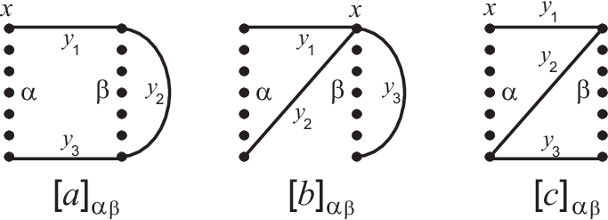
We now turn to the two-loop corrections. The three different sets of diagrams contributing to elasticity are depicted in Fig. 3. The details of calculations are given in the Appendix. Summing up all contributions, we arrive at

To render the poles in $\varepsilon$ and $\delta$, we introduce the renormalization group Z factor as follows:

The exponent $\psi$ is given then by

where subscript 0 indicates a derivative at constant bare parameters. Taking the derivative with respect to the mass, we obtain

To calculate $\psi$, we have to express the bare disorder via renormalized one as follows:

Substituting Eq. (29) in Eq. (28), we find that the leading two-loop corrections are exactly canceled by the counter-terms, so that we leave with

The finite part of the single-replica two-loop diagrams (25) is expected to correct elasticity at three-loop order. Hence, we argue that the perturbation theory for this model is organized in such a way that the single-replica $p$-loop diagrams correct the elasticity only to $(p+1)$ order. Since $R_{2}(u)$ remains analytic along the FRG flow, we have $R^{(4)}_{2}(0)>0$, and therefore, $\psi<0$. The corresponding values of the exponent $\psi$ computed for the RF, RB, and RP universality classes using the FPs found in Ref. fedorenko-pre-2006a are shown in Fig. 4.

We now show how one can calculate the roughness exponent $\zeta$ to second order in $\varepsilon$ and $\delta$ knowing only the exponent $\psi$ computed to second order in Sec. III.3. To that end, we do not need the whole FRG to two-loop order. Let us start with the RB universality class. The roughness exponent is fixed by a stable RB FP solution of Eqs. (20) and (21) which decays exponentially fast for large $u$. The equations possess both the SR RB FP with $R_{2}(u)=0$ and the LR RB FP with $R_{2}(u)\neq 0$. The roughness exponent corresponding to the SR RB FP is known to second order in $\varepsilon$ and readschauve01; ledoussal04

Despite the smallness of the two-loop correction, the estimation of the exponent in $d=1$, $\zeta_{\mathrm{SRRB}}=0.6866$ given by Eq. (31), visibly differs from the known exact result $2/3$. One can improve the accuracy of $\zeta$ by use the Padé approximant [2/1] involving also the unknown third order correction. Tuning the latter in order to reproduce the exact result $2/3$ for $\varepsilon=3$, we end up with the expression

which is expected to be fairly accurate for $0\leq\varepsilon\leq 3$.

We now focus on the LR RB FP with $R_{2}(u)\neq 0$. We can integrate both sides of flow equation (21) over $u$ from $0$ to $\infty$ taking into account that for RB disorder $R_{2}(u)$ decays exponentially fast. Since for RB disorder the integral $\int_{0}^{\infty}du\,R_{2}(u)$ is nonzero, we can determine the roughness exponent $\zeta_{\mathrm{LRRB}}=\delta/5$ to first order in $\varepsilon$ and $\delta$. Fortunately, one can go beyond the one-loop approximation. Indeed, the direct inspection of diagrams contributing to the flow equation (21) shows that the higher orders can only be linear in even derivatives of $R_{2}(u)$. The only term which is linear in $R_{2}(u)$ comes from the renormalization of elasticity and can be rewritten as $2\psi R_{2}(u)$ to all orders. Hence, we have to all orders

and as a consequence, $\int_{0}^{\infty}duR_{2}(u)$ is exactly preserved along the FRG flow resulting in the exact identity

Substituting Eq. (30) into Eq. (34), we obtain the roughness exponent $\zeta_{\mathrm{LRRB}}$ to second order in $\varepsilon$ and $\delta$. Before we proceed to compute the exponents, let us to check stability of the SR and LR RB FPs. As was shown in Ref. fedorenko-pre-2006a, the SR RB FP is unstable with respect to LR disorder if $\zeta_{\mathrm{LRRB}}>\zeta_{\mathrm{SRRB}}$. To one-loop order, this gives that the SR RB FP is stable for $\delta<1.0415\varepsilon$. Equating (34) and (32), we can compute the stability regions to second order in $\varepsilon$ and $\delta$ (see Fig. 5). The alternative way to determine the crossover line relies on the requirement that the exponent $\psi$ is a continuous function of $\varepsilon$ and $\delta$. It is zero in the region controlled by the SR FP, and therefore has to vanish when approaching the crossover line from the LR stability region. Since the $\psi$ is of second order in $\varepsilon$ and $\delta$, the $\psi$ criterion at two-loop order gives the same stability regions as the roughness exponents equating at one-loop order. However, we can significantly improve the latter if we take into account that $\psi=0$ on the crossover line. The resulting crossover line is shown in Fig. 5. We can also improve the two-loop estimation of $\psi$. To that end, we write down a formal expansion of $\psi$ in $\varepsilon$,

The function $f_{1}(x)$ is basically the function shown in Fig. 4. We now tune the function $f_{2}(x)$ in order to make $\psi=0$ on the crossover line and find

Using Eqs. (35) and (36), we compute the roughness exponent $\zeta_{\mathrm{LRRB}}$ as a function of $\delta$ for $\varepsilon=1$ and $\varepsilon=2$ (see Fig. 6). Unfortunately, the accuracy rapidly decays with $\varepsilon$, so that estimation of the roughness exponent for $\varepsilon=3$ is very difficult and postponed to Sec. V.

Similar to the case of RB disorder, one can show that the roughness exponent at the LR RF FP is exactly given by

and the crossover line between the SR and LR RF FPs is exactly given by $\delta=\varepsilon$.

Here, we extend the previous one-loop FRG studiesbalents93; chauvethesis of elastic systems in the presence of columnar disorder to two-loop order and proceed to describe the transverse Meissner physics in a quantitative way. We consider the model with $\varepsilon_{d}$-dimensional extended defects introduced in Sec. II.1. We take $c_{i}=c_{\parallel}$ $(i=1,...,\varepsilon_{d})$ and we are also free to put $c_{i}=1$ $(i=\varepsilon_{d}+1,...,d)$ since they do not get corrected by disorder. Simple power counting shows that the upper critical dimension of the problem is $d_{\mathrm{uc}}=4+\varepsilon_{d}$. We use the dimensional regularization of integrals with a $\tilde{\varepsilon}=4-d+\varepsilon_{d}$ expansion. The FRG flow equations to two-loop order read

where $\theta_{T}=d-2+2\zeta$ and $\Lambda_{0}$ is the bare cutoff. In Eq. (45), $\tilde{h}$ is the coefficient in front of the term

ultimately generated in the effective Hamiltonian along the FRG flow.balents93 The correction to $\tilde{h}$ is strongly UV diverging, and thus is nonuniversal. Note that the flow equation for the generalized columnar disorder (42) coincides to all orders with that for pointlike disorder up to change $\tilde{\varepsilon}\to\varepsilon$.

Let us start from the analysis at $T=0$. The flow picture very resembles that for the depinning transition with tilt $\vartheta$, longitudinal elasticity $c_{\parallel}$, and tilting field $h$ playing the roles of velocity, friction, and driving force, respectively. For $d<4+\varepsilon_{d}$, the running disorder correlator $R^{(4)}(u)$ blows up at the Larkin scale

Consequently, the longitudinal elasticity diverges at zero tilt $\vartheta$ in a way similar to mobility divergence at the depinning transition in quasistatic limit. Beyond the Larkin scale $l>l_{c}$, the $R^{(2)}(u)$ develops a cusp at origin, $R^{\prime\prime\prime}(0^{+})>0$. The term (46) is generated in the effective Hamiltonian and the $R^{(4)}(0)$ changes its sign from positive to negative. The latter leads to a power law decay of the longitudinal elasticity $c_{\parallel}\propto L^{-\psi}$ with

where $R^{*}(u)$ is a FP solution of the flow equation (42). Similar to the threshold force generation at the depinning transition, term (46) reduces the tilting force and generates the critical tilting force $h_{c}$. The flow equation (45) allows us to estimate the nonuniversal value of $h_{c}$. Integrating Eq. (45) up to large scales, we find

We now in a position to compute the exponent $\phi$, which we define as

To that end, we renormalize the equilibrium balance equation $h-h_{c}=c_{1}(L)\vartheta$ up to the scale $L=\xi_{\vartheta}$ at which the elasticity $c_{1}$ stops to get renormalized. Using Eq. (41), we obtain the exact scaling relation

The exponents $\zeta$, $\psi$, and $\phi$ computed to second order in $\tilde{\varepsilon}$ for different universality classes are summarized in Tab. 1. Note that expansions in $\tilde{\varepsilon}$ are expected to be Borel nonsummable, and thus ill behaved for high orders and large $\tilde{\varepsilon}$. In this light, the using of exact relation (51) may be more favorable than the expansions given in the last column of Table 1. Systems described by the RP universality class exhibit slow logarithmic growth of displacements

where $\bar{u}_{x_{\perp}}:=L^{-\varepsilon_{d}}\int d^{\varepsilon_{d}}x_{\parallel}\,u_{x}$. The universal amplitude can be easily deduced from the results for the uncorrelated disorder and to two loop reads

where we have fixed the period to $1$. The logarithmic growth of displacements corresponds to a slow power-law decay of the translation order, and thus should lead to Bragg peaks unexpected for a strongly pinned Bose-glass. The system under consideration shares features of the Bragg glass, such as power-law decay of the translation order, and the strong Bose glass, namely, the diverging tilt modulus (transverse Meissner effect). One can expect this behavior for a weak Bose-glass which is pinned collectively. Recently, such a glassy phase called Bragg-Bose glass was observed in numerical simulations of vortices in bulk superconductor at low concentrations of columnar disorder and low temperatures.nonomura04; dasgupta05

A finite temperature $T>0$ rounds the cusp of the running disorder correlator $R_{l}(u)$, so that in the boundary layer $u\sim T_{l}$, it significantly deviates form the FP solution and obeys the following scaling form:chauve-00

where $\chi=|R^{*\prime\prime\prime}(0)|$. However, as was pointed in Ref. chauvembg the flow equations for columnar disorder have a remarkable feature in comparison with uncorrelated disorder. Indeed, substituting the boundary layer scaling (54) in the temperature flow equation (44), we obtain

As follows from Eq. (55), the effective temperature $T_{l}$ vanishes at a finite length scale $L_{\mathrm{loc}}=e^{l_{\mathrm{loc}}}/\Lambda_{0}$,

so that the localization effects are settled only on scales larger than $l_{\mathrm{loc}}>l_{c}$.

Let us discuss the special case of flux lines in (1+1) dimensions which the qualitative phase diagram is shown in Fig. 1. The transverse Meissner physics for collectively pinned weak Bose glass and small tilt angles $\vartheta=B_{\perp}/B_{\parallel}$ can be explored using the results obtained in the previous section for the RP universality class with $\tilde{\varepsilon}=4-2+1=3$. Here, we restore the dependence on the flux line density $n_{0}$ fixing the period of $R(u)$ to $1/n_{0}$. In contrast to the Bragg-glass, the weak Bose-glass survives in $d=2$. Indeed, for uncorrelated disorder in $d=2$, the temperature turns out to be marginally relevant, so that the system has a line of FPs describing a super-rough phase with anomalous growth of the two-point correlation $\overline{(u_{x}-u_{0})^{2}}=A(T)\ln^{2}x+O(\ln x)$.schehr07 According to Eqs. (55) and (56) for columnar disorder the temperature vanishes at finite, though a very large scale

Unfortunately, the large value of $\tilde{\varepsilon}$ makes estimation of $\phi$ extremely unreliable. Indeed, the expansion in $\tilde{\varepsilon}$ shown in Table 1 leads to a zero value of $\phi$. The exact scaling relation (51) with $\psi$ computed using the expression from Table 1 gives

The one-loop result reproduces the estimation $\phi=1/2$ given by heuristic random walk arguments based on the entropy of flux lines wandering in the presence of thermal fluctuations.hwa93 The model of vortices wandering in a random array of columnar defects can be mapped onto a quantum problem of disordered bosons.nelson92 One can regard each vortex as an imaginary time world line of a boson, so that the columnar pins parallel to vortices become quenched pointlike disorder in the quantum problem. The transverse magnetic field $H_{\perp}$ will play the role of an imaginary vector potential $h$ for the bosons,affleck04 so that the bosonic Hamiltonian turns out to be non-Hermitian:

References

- (1) S. Lemerle, J. Ferre, C. Chappert, V. Mathet, T. Giamarchi, and P. Le Doussal, Phys. Rev. Lett. 80, 849 (1998).
- (2) G. Grüner, Rev. Mod. Phys. 60, 1129 (1988).
- (3) G. Blatter, M.V. Feigel’man, V.B. Geshkenbein, A.I. Larkin, and V.M. Vinokur, Rev. Mod. Phys. 66, 1125 (1994).
- (4) D. S. Fisher, Phys. Rep. 301, 113 (1998).
- (5) M. Kardar, Phys. Rep. 301, 85 (1998).
- (6) S. Brazovskii and T. Nattermann, Adv. Phys. 53, 177 (2004).
- (7) T. Giamarchi and P. Le Doussal, Phys. Rev. Lett. 72, 1530 (1994); Phys. Rev. B 52, 1242 (1995).
- (8) L. Civale, A.D. Marwick, T.K. Worthington, M.A. Kirk, J.R. Thompson, L. Krusin-Elbaum, Y. Sun, J.R. Clem, and F. Holtzberg, Phys. Rev. Lett. 67, 648 (1991).
- (9) D.R. Nelson and V.M. Vinokur, Phys. Rev. Lett. 68, 2398 (1992).
- (10) L. Radzihovsky, Phys. Rev. Lett. 74, 4923 (1995).
- (11) A.W. Smith, H.M. Jaeger, T.F. Rosenbaum, W.K. Kwok, and G.W. Crabtree, Phys. Rev. B 63, 064514 (2001).
- (12) T. Hwa, D.R. Nelson, and V.M. Vinokur, Phys. Rev. B 48, 1167 (1993).
- (13) R.J. Olsson, W.K. Kwok, L.M. Paulius, A.M. Petrean, D.J. Hofman, and G.W. Crabtree, Phys. Rev. B 65, 104520 (2002).
- (14) G. Refael, W. Hofstetter, and D.R. Nelson, Phys. Rev. B, 74, 174520 (2006).
- (15) M. Mezard and G. Parisi, J. Phys. A 23, L1229 (1990).
- (16) D. S. Fisher, Phys. Rev. Lett. 56, 1964 (1986).
- (17) A.I. Larkin, Sov. Phys. JETP 31, 784 (1970).
- (18) T. Nattermann, S. Stepanow, L.-H. Tang, and H. Leschhorn, J. Phys. II 2, 1483 (1992).
- (19) H. Leschhorn, T. Nattermann, S. Stepanow, and L.-H. Tang, Ann. Phys. 6, 1 (1997).
- (20) O. Narayan and D. S. Fisher, Phys. Rev. B 48, 7030 (1993).
- (21) A.A. Fedorenko and S. Stepanow, Phys. Rev. E 67, 057104 (2003).
- (22) P. Chauve, P. Le Doussal, and K.J. Wiese, Phys. Rev. Lett. 86, 1785 (2001).
- (23) P. Le Doussal, K.J. Wiese, and P. Chauve, Phys. Rev. B 66, 174201 (2002).
- (24) P. Le Doussal, K.J. Wiese, and P. Chauve, Phys. Rev. E 69, 026112 (2004).
- (25) P. Le Doussal, M. Mueller, and K.J. Wiese, Phys. Rev. B 77, 064203 (2008).
- (26) L. Roters and K.D. Usadel, Phys. Rev. E 65, 027101 (2002)
- (27) L. Roters, S. Lübeck, and K. D. Usadel, Phys. Rev. E 66, 026127 (2002).
- (28) A. Rosso, A.K. Hartmann, and W. Krauth, Phys. Rev. E 67, 021602 (2003).
- (29) A. Rosso, W. Krauth, P. Le Doussal, J. Vannimenus, and K.J. Wiese, Phys. Rev. E 68, 036128 (2003).
- (30) A.A. Fedorenko, P. Le Doussal, and K.J. Wiese, Phys. Rev. E 74, 041110 (2006).
- (31) A.A. Middleton, P. Le Doussal, and K.J. Wiese, Phys. Rev. Lett. 98, 155701 (2007); P. Le Doussal and K.J. Wiese, EPL 77, 66001 (2007); A. Rosso, P. Le Doussal, and K.J. Wiese, Phys. Rev. B 75, 220201(R) (2007).
- (32) L. Balents, Europhys. Lett. 24, 489 (1993).
- (33) P. Chauve, P. Le Doussal, and T. Giamarchi, Phys. Rev. B 61, R11906(2000).
- (34) P. Chauve, Ph.D. thesis, Université de Paris XI Orsay, 2000; http:/www.lpt.ens.fr/ chauve/
- (35) A.A. Fedorenko, P. Le Doussal, and K.J. Wiese, Phys. Rev. E 74, 061109 (2006).
- (36) S.N. Dorogovtsev, Phys. Lett. 76A, 169 (1980).
- (37) D. Boyanovsky and J.L. Cardy, Phys. Rev. B 26, 154 (1982).
- (38) A.A. Fedorenko, Phys. Rev. B 69, 134301 (2004).
- (39) A. Weinrib and B.I. Halperin, Phys. Rev. B 27, 413 (1983).
- (40) E. Korutcheva and F. Javier de la Rubia, Phys. Rev. B 58, 5153 (1998).
- (41) V.V. Prudnikov and A.A. Fedorenko, J. Phys. A 32, L399 (1999); V.V. Prudnikov, P.V. Prudnikov, and A.A. Fedorenko, ibid. 32, 8587 (1999); Phys. Rev. B 62, 8777 (2000).
- (42) A.A. Fedorenko and F. Kühnel, Phys. Rev. B, 75, 174206 (2007).
- (43) Y. Yamazaki, A. Holz, M. Ochiai, and Y. Fukuda, Physica A 150, 576 (1988).
- (44) Y. Nonomura and X. Hu, Europhys. Lett. 65, 533 (2004).
- (45) C. Dasgupta and O.T. Valls, Phys. Rev. B 72, 094501 (2005).
- (46) P. Chauve, T. Giamarchi, and P. Le Doussal, Phys Rev. B 62, 6241 (2000).
- (47) J.L. Cardy and S. Ostlund, Phys. Rev. B 25, 6899 (1982); P. Le Doussal and G. Schehr, ibid. 75, 184401 (2007).
- (48) I. Affleck, W. Hofstetter, D.R. Nelson, and U. Schollwock, J. Stat. Mech.: Theory Exp. 2004, P10003.
- (49) F.D.M. Haldane, Phys. Rev. Lett. 47, 1840 (1981).
- (50) J.P. Rodriguez and M.P. Maley, Phys. Rev. B 73, 094502 (2006); J.P. Rodriguez, ibid. 76, 224502 (2007).
- (51) M. Kardar, G. Parisi, and Y.-C. Zhang, Phys. Rev. Lett. 56, 889 (1986).
- (52) E. Medina, T. Hwa, M. Kardar, and Y.-C. Zhang, Phys. Rev. A 39, 3053 (1989).
- (53) C.-H. Lam, L.M. Sander, and D.E. Wolf, Phys. Rev. A 46, R6128 (1992).
- (54) E. Katzav and M. Schwartz, Phys. Rev. E 70, 011601 (2004).