1 Relative percentage error is plotted as a function of z for = Ω v 0.7 . Notice that the error decreases sharply up to = z 1 and more slowly afterwards. For = z 1 , the relative error is about % 0.055 . For = z 5 , the error is about % 0.023 .

AN APPROXIMATE ANALYTICAL ALGORITHM FOR EVALUATING THE DISTANCES IN A DARK ENERGY DOMINATED UNIVERSE

T. Wickramasinghe

Department of Physics, The College of New Jersey, Ewing, NJ 08628

Email: wick@beast.tcnj.edu

ABSTRACT

The most recent cosmological observations indicate that the present universe is flat and vacuum dominated. In such a universe, the distance measurements are always difficult and involve numerical computations. In this paper, it is shown that the most fundamental distance measurement of cosmology, the luminosity distance, for such a universe can be obtained in an approximate analytical way with very small errors of less than $0.02\%$ up to vacuum energy. The analytical calculation is shown to be exceedingly efficient, as compared to the traditional numerical methods.

1. INTRODUCTION

The most recent cosmological observations indicate that the present universe is flat and vacuum dominated such that $\Omega_{v}\approx 0.7$ . In a such a vacuum dominated spacetime, the distance analysis is difficult and time consuming. In this paper it is shown that the luminosity distance $D_{L}$ can be obtained to a high degree of accuracy in a purely simple, analytical way. The analytical calculation is shown to be exceedingly efficient and has a relative error of less than $0.02\%$ at a redshift of $5$ , as compared to numerical methods. The analytical calculation can be performed in any reasonable computer system and runs very fast.

Current astronomical observations indicate that the present density parameter of the universe is $\Omega_{v}+\Omega_{m}=1$ and that $\Omega_{v}\approx 0.7$ , where $\Omega_{m}$ is the contribution from all the fields other than the vacuum. Thus, the calculations of distances in such a vacuum dominated universe becomes very important. However, the distance calculations in such a vacuum dominated universe involve repeated numerical calculations and elliptic functions (Einstein 1997). In order to simplify the numerical calculations, Pen (Pen 1999) has developed quite an efficient analytical recipe.

In this paper, I show that a quite an elegant analytical method, similar in many respect to that of Pen, can be developed to calculate the distances in a vacuum dominated flat universe. The analytical calculation is shown to run faster than that of Pen and has smaller errors that become insignificant as $z$ increases. The paper is organized as follows. In §2, I will develop a theory to deduce the luminosity distance from first principles. In §3, I will derive necessary tools for the analysis of errors in the analytical approach and will show that the errors at $z=1$ are of the order of $0.05\%$ , which is decreasing even further as the redshift $z$ increases beyond unity, making the analytical algorithm exceedingly efficient.

2. THEORY

The most fundamental distance scale in the universe is the luminosity distance defined by $D_{L}=\sqrt{L/4\pi F_{0}}$ , where $F_{0}$ is the observed flux of an astronomical object having a luminosity $L$ .

We first begin by analyzing how the scale factor $R(t)$ varies as a function of time $t$ in a flat universe in which $\Omega_{v}\neq 0$ . In this case, $\dot{R}(t)$ is given by (Narlikar 1983).

{\dot{R}}^{2}=H_{0}^{2}\Omega_{v}R^{2}+H_{0}^{2}\Omega_{m}{R_{0}^{3}\over{R}}

(1)

The foregoing is immediately integrated into

\left({R\over{R_{0}}}\right)^{3}={1\over{2}}{\Omega_{m}\over{\Omega_{v}}}\left[\cosh\left(3H_{0}t\sqrt{\Omega_{v}}\right)-1\right]

(2)

Let us define $x=3\sqrt{\Omega_{v}}H_{0}t$ and indicate its present value by $x_{0}$ . Then, Eq (2) gives

x=x(z,\Omega_{v})=\cosh^{-1}\left[1+2{\Omega_{v}\over{1-\Omega_{v}}}{1\over{(1+z)^{3}}}\right]

(3)

We note that $x$ is a monotonically decreasing function beyond $x_{0}=x(0,0.7)=2.5$ . We choose the standard Robertson-Walker metric (Peacock 1999) as the metric of the background spacetime. With usual notations, this is

ds^{2}=c^{2}dt^{2}-R^{2}\left[{dr^{2}\over{1-kr^{2}}}+r^{2}(d\theta^{2}+\sin^{2}\theta d\phi^{2})\right]

(4)

In the above spacetime, we can use Eq (2) to obtain $r$ . A simple integration for a flat universe $(k=0)$ yields,

r={c\over{H_{0}}R_{0}}{1\over{3\,\Omega_{v}^{1\over 6}\Omega_{m}^{1\over 3}}}\int\limits_{x}^{x_{0}}{dx^{\prime}\over{\left[\sinh{x^{\prime}\over 2}\right]^{2\over 3}}}

(5)

We now define a new function $\Psi(x)=\lim_{\delta\rightarrow 0}\int\limits_{\delta}^{x}{dx^{\prime}/{\left[\sinh{x^{\prime}/2}\right]^{2\over 3}}}$ .

In the standard model the luminosity distance is defined as $D_{L}=rR_{0}(1+z)$ . Now we can use Eq (5) to write the luminosity distance as

D_{L}={c\over{3H_{0}}}{1+z\over{\Omega_{v}^{1\over 6}\Omega_{m}^{1\over 3}}}\left[\Psi(x_{0})-\Psi(x)\right]

(6)

Expanding $\Psi$ in a series expansion to the 4th order, we find that

\Psi(x)=3\;2^{{2\over 3}}x^{{1\over 3}}\left[1-{x^{2}\over 252}+{x^{4}\over 21060}\right]+\Psi(0)

(7)

where $\Psi(0)=-2.210$ . Now, Eq (6) reduces to the required expression for the luminosity distance as

D_{L}={c\over{3H_{0}}}{1+z\over{\Omega_{v}^{1\over 6}{(1-\Omega_{v})}^{1\over 3}}}\left[\Psi(x_{0})-\Psi(x)\right]

(8)

3. CONCLUSIONS

Eq (8) is the general form for $D_{L}$ in a vacuum dominated universe. The most popular flat model is the the one in which $\Omega_{m}=\Omega_{0}=1$ . We find that our model goes very smoothly over to the luminosity distance in a flat model in which $\Omega_{v}=0$ .

Refer to caption — Figure 1: Relative percentage error is plotted as a function of $z$ for $\Omega_{v}=0.7$ . Notice that the error decreases sharply up to $z=1$ and more slowly afterwards. For $z=1$ , the relative error is about $0.055\%$ . For $z=5$ , the error is about $0.023\%$ .

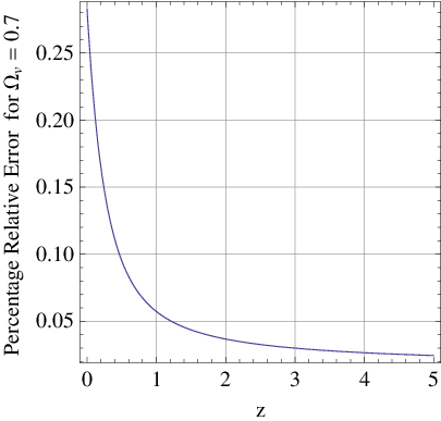
The luminosity distance steadily increases as the redshift $z$ . Thus in order to get a better distance estimate, it is important to check the possible errors that might have crept into the analytical approximation in Eq (8).

The analysis was done using Eq (7). The numerical simulations infer that there exists a relatively small error in our method. Our calculation shows that the error rapidly drops as $z$ increases. The error at $z=1$ is is estimated to be $<0.05\%$ . At $z=5$ , $x=0.207$ and the error is about $0.023\%$ . For large $z$ , the error becomes exceedingly small.

Therefore, our analytical method becomes quite desirable as the most interesting astronomical phenomena happen at $z>1$ , for which the errors in our method can safely be neglected. Furthermore, the analytical computation is more elegant and faster compared to traditional numerical computations invoked in connection with calculations of distances in a vacuum dominated universe.

Once we know the luminosity distance, it becomes a simple matter to evaluate the other distances such as the angular diameter distance and proper distance.

I thank the anonymous referee for constructive suggestions and improvements.

4. REFERENCES

Einstein, D. 1997, astro-ph/9709054

Narlikar, J. V. 1983, Introduction to Cosmology, Cambridge

Peacock, J. A. 1999, Cosmological Physics, Cambridge, 69

Pen, U. 1999, ApJ Supplement Series, 120, 49

Weinberg, S. 1972, Gravitation & Cosmology, Weily