Infrared finite ghost propagator in the Feynman gauge
Abstract
We demonstrate how to obtain from the Schwinger-Dyson equations of QCD an infrared finite ghost propagator in the Feynman gauge. The key ingredient in this construction is the longitudinal form factor of the non-perturbative gluon-ghost vertex, which, contrary to what happens in the Landau gauge, contributes non-trivially to the gap equation of the ghost. The detailed study of the corresponding vertex equation reveals that in the presence of a dynamical infrared cutoff this form factor remains finite in the limit of vanishing ghost momentum. This, in turn, allows the ghost self-energy to reach a finite value in the infrared, without having to assume any additional properties for the gluon-ghost vertex, such as the presence of massless poles. The implications of this result and possible future directions are briefly outlined.
pacs
12.38.Lg, 12.38.AwI Introduction
The non-perturbative properties of the basic Green’s functions of QCD have been the focal point of intensive scrutiny in recent years, with particular emphasis on the propagators of the fundamental degrees of freedom, gluons, quarks, and ghosts. Even though it is well-known that these quantities are not physical, since they depend on the gauge-fixing scheme and parameters used to quantize the theory, it is generally accepted that reliable information on their non-perturbative structure is essential for unraveling the infrared (IR) dynamics of QCD.
There are two main tools usually employed in this search: the lattice, where space-time is discretized and the quantities of interest are evaluated numerically Creutz:1980zw; Mandula:1987rh; Bernard:1993tz, and the intrinsically non-perturbative equations governing the dynamics of the Green’s functions, known as Schwinger-Dyson equations (SDE) Dyson:1949ha; Schwinger:1951ex; Cornwall:1974vz; Marciano:1977su. In principle, the lattice includes all non-perturbative features and no approximations are employed at the level of the theory. In practice, the main limitations appear when attempting to extrapolate the results obtained with finite lattice volume to the continuous space-time limit. On the other hand, the main difficulty with the SDE has to do with the need to devise a self-consistent truncation scheme that preserves crucial field-theoretic properties, such as the transversality of the gluon self-energy, known to be valid both perturbatively and non-perturbatively, as a consequence of the BRST symmetry Becchi:1975nq.
Significant progress has been accomplished on this last issue due to the development of the truncation scheme that is based on the all-order correspondence Binosi:2002ft between the pinch technique (PT) Cornwall:1981zr; Cornwall:1989gv and the Feynman gauge of the Background Field Method (BFM) Abbott:1980hw. One of its most powerful features is the special way in which the transversality of the gluon self-energy is realized. Specifically, by virtue of the Abelian-like WIs satisfied by the vertices involved, gluonic and ghost contributions are separately transverse, within each order in the “dressed-loop” expansion of the SDE Aguilar:2006gr for the gluon propagator. This property, in turn, allows for a systematic truncation of the full SDE, preserving at every step the crucial property of gauge invariance.
The first approximation to the SDE of the gluon propagator involves the one-loop dressed gluonic graphs only, since in this scheme the ghost loops may be omitted without compromising the transversality of the answer. As is well-known, the Feynman gauge of the BFM is particularly privileged, being dynamically singled out as the gauge that directly encompasses the relevant gauge cancellations of the PT Binosi:2002ft. Therefore, the aforementioned one-loop dressed graphs have been considered in this particular gauge. The detailed study of the resulting integral equation for the gluon propagator gave rise to solutions that reach a finite value in the deep IR Aguilar:2006gr; Aguilar:2007ie. Following Cornwall’s original idea Cornwall:1979hz; Cornwall:1981zr of describing the IR sector of QCD in terms of an effective gluon mass Bernard:1981pg; ref, these solutions have been fitted using “massive” propagators of the form , with , and the crucial characteristic that is not “hard”, but depends non-trivially on the momentum transfer . In addition, finite solutions for the gluon propagator in the Landau gauge have been reported in various lattice studies Alexandrou:2000ja, and were recently confirmed using lattices with significantly larger volumes Cucchieri:2007md.
Even though the omission of the ghost loops within this formulation does not introduce any artifacts, such as the loss of transversality, the actual behavior of the ghosts may change the initial prediction for the gluon propagator, not just quantitatively but also qualitatively. For example, an IR divergent solution for the ghost propagator could destabilize the finite solutions found for the gluon propagator. Therefore, a detailed study of the ghost sector constitutes the next challenge in this approach. In the present work we will consider the SDE for the ghost sector in the (BFM) Feynman gauge, in order to complement the corresponding analysis presented in Aguilar:2006gr; Aguilar:2007ie in the same gauge. The BFM Feynman rules are in general different to those of the covariant renormalizable gauges Abbott:1980hw; in the former, for example, in addition to the bare gluon propagator, the bare three- and four-gluon vertices involving background and quantum gluons depend on the (quantum) gauge fixing parameter. Notice, however, that, since there are no background ghosts, the Feynman rules relevant for the ghost sector are identical to both the covariant gauges and the BFM. Therefore, the analysis and the results presented in this article carries over directly to the conventional Feynman gauge.
In this article we demonstrate that the ghost propagator in the Feynman gauge can be made finite in the IR, through the self-consistent treatment of the gluon-ghost vertex and the ghost gap equations. The key ingredient that makes this possible is the “longitudinal” form-factor in the tensorial decomposition of the gluon-ghost vertex, , i.e. the co-factor of , where is the four-momentum of the gluon; evidently this term gets annihilated when contracted with the usual transverse projection operator. As we will explain in detail, this component acquires a special role for all values of the gauge fixing parameter, with the very characteristic exception of the Landau gauge. The reason is simply that in the Landau gauge the entire gluon propagator is transverse, both its self-energy and its free part, whereas for any other value of the gauge-fixing parameter the free part is not transverse. As a result, when the gluon-ghost vertex is inserted into the SDE for the ghost propagator, , its part proportional to dies when contracted with the gluon propagator in the Landau gauge; however, in any other gauge it survives due to the free-part of the gluon propagator. The resulting contribution has the additional crucial property of not vanishing as the external momentum of the ghost goes to zero. Therefore, contrary to what happens in the Landau gauge where only the part of the vertex proportional to survives, one does not need to assume the presence of massless pole terms of the form in order to obtain a nonvanishing value for . Instead, the only requirement is that the longitudinal form factor simply does not vanish in that limit.
The paper is organized as follows: In section II we set up the SDE for the ghost propagator, assuming the most general Lorentz structure for the fully dressed gluon-ghost vertex . We then discuss under what condition the resulting expression may yield a finite value for , and analyze the profound differences between the Landau and the Feynman-type of gauges. In section III we first derive the gluon-ghost vertex under certain simplifying assumptions, discuss in detail the approximations employed. Next we study its non-perturbative solutions employing various physically motivated, IR finite Ansätze IR for the gluon and ghost propagators. In Section IV we combine the results of the previous two sections, deriving the self-consistency condition necessary for the system of equations to be simultaneously satisfied. Finally, in section V we discuss our results and present our conclusions.
II General considerations on the IR behavior of the ghost
In this section we derive the SDE for the ghost propagator in a general covariant gauge, and study qualitatively its predictions for for various gauge choices. In particular, we establish that away from the Landau gauge the ghost propagator may acquire a finite value at the origin, without the need to assume a singular IR behavior for the form factors of the fully dressed ghost-gluon vertex entering into the SDE. Our attention will eventually focus on the Feynman gauge, which, as mentioned in the Introduction, is singled out within the PT-BFM scheme.
The full ghost propagator is usually written in the form
| (2.1) |
and the SDE satisfied by , depicted diagrammatically in Fig.1, reads
| (2.2) |
We have used , with the Casimir eigenvalue in the adjoint representation [ for ], and have introduced the short-hand notation , where is the dimension of space-time used in dimensional regularization. is the fully dressed gluon propagator, whereas denotes the fully dressed gluon-ghost vertex and its tree-level value.

Specifically, in the covariant gauges the full gluon propagator has the general form
| (2.3) |
where
| (2.4) |
is the transverse projector, and is the gauge fixing parameter; corresponds to the Feynman gauge and to the Landau gauge. The scalar function is related to the all-order gluon self-energy ,
| (2.5) |
through
| (2.6) |
The bare gluon-ghost vertex appearing in (2.2) is given by , with (). Choosing and as the two linearly independent four-vectors, the most general decomposition for the fully dressed gluon-ghost vertex is expressed as Pascual:1980yu
| (2.7) |
where is the outgoing gluon momentum, and , the outgoing and incoming ghost momenta, respectively. The dimensionless scalar functions and are the form factors of the gluon-ghost vertex. In particular, notice that the tree-level result is recovered when we set and . Finally, it is important to emphasize that all fully-dressed scalar quantities (, , , and ) depend explicitly (and non-trivially) on the value of the gauge-fixing parameter already at the level of one-loop perturbation theory.
It is then straightforward to derive the Euclidean version of Eq.(2.2); to that end, we set , define , and , and for the integration measure we have . Suppressing the subscript “E” everywhere except in the integration measure, and without any assumptions on the functional form of and , the ghost SDE of Eq. (2.2) becomes
| (2.8) | |||||
As a check, we can recover from (2.8) the one-loop result for the ghost propagator in the Feynman gauge () by substituting the tree-level expressions for the ghost and gluon propagators and setting and ; specifically
| (2.9) |
In order to obtain from (2.8) the behavior of for the full range of the momentum one needs to provide additional information for the forms factors and , obtained from the corresponding SDE satisfied by the gluon-ghost vertex. Thus, the complete treatment of this problem would require the solution of a complicated system of coupled SDE. However, several interesting conclusions about the IR behavior of may be drawn, by considering the qualitative behavior of the forms factors and , as .
We start by considering what happens in the Landau gauge. First of all, let us assume that the various quantities appearing on the r.h.s. of (2.8) are regular functions of foot1. Then, if we set , only the first integral on the r.h.s. of (2.8) survives; thus, is only affected by the functional form of . In particular, the behavior of as will depend on whether is divergent or finite in that limit, i.e. on whether or not contains terms. Evidently, if does not contain poles, one has that , and therefore the ghost propagator will be divergent in the IR. On the other hand, if contains terms, allowing for finite solutions for the ghost propagator.
According to this general argument, the only way for getting an IR-finite propagator in the Landau gauge is by assuming that contains poles Fischer:2006ub; Boucaud:2007va. However, lattice simulations in the Landau gauge seem to favor a IR-finite ; specifically, it was found that deviations of the gluon-ghost vertex from its tree-level value are very small in the IR, i.e. Cucchieri:2004sq. In addition, a detailed study of the SDE equation for in the same gauge shows no singular behavior for Schleifenbaum:2004id . These findings appear to be consistent with recent lattice results on the non-perturbative structure of the ghost propagator, which indicate that in the Landau gauge diverges, at a rate that deviates only mildly from the tree-level expectation of Cucchieri:2007md.
Evidently, the picture for is drastically different. Indeed, away from the Landau gauge the r.h.s of (2.8) involves both form factors, and . Moreover, unlike the first two terms, the third one does not contain any kinematic factors proportional to . Thus, in order for it not to vanish as one does not need to assume any singular structure for ; instead, it is sufficient to simply have that .
After this key observation, we will take the limit of of Eq. (2.8) as , assuming that does not contain terms. Focusing for concreteness on the physically relevant case of , we find that in the aforementioned kinematic limit Eq.(2.8) reduces to
| (2.10) |
Of course, if the assumption that is regular as does not hold, then the other integrals will also contribute to the r.h.s. of (2.10). However, modulo the rather contrived scenario of fine-tuned cancellations, the r.h.s. will still be different from zero. Evidently, from (2.10) we deduce that if than . On the other hand, if , i.e. if it does not vanish identically, then one may have a non-vanishing . Of course, having a non-vanishing is not a sufficient condition for ; one has to assume in addition that (i) the integral on the r.h.s. of (2.10). is convergent, or it can be made convergent through proper regularization, and (ii) that the integral is not zero due to some other, rather contrived circumstances (for instance, if turned out not to be a monotonic function, the various contributions from different integration regions could cancel against each other).
An explicit calculation may confirm that vanishes at one-loop Watson:1999ha, and it is reasonable to expect this to persist to all orders in perturbation theory. Therefore, in what follows we will examine the possibility that may not vanish non-perturbatively. In particular, we will study the SDE determining for the special kinematic configuration appearing in (2.10), namely where the outgoing ghost momentum, , is set equal to zero (i.e. and ). In the context of the linearized approximation that we employ in the next section this kinematic configuration offers the particular technical advantage of dealing with a function of only one variable instead of two.
III The gluon-ghost vertex
In this section we set up and solve, after certain simplifying approximations, the SDE governing the behavior of the form factor . This can be done by taking the following limit of the gluon-ghost vertex, ,
| (3.1) |
where obeys the SDE Marciano:1977su represented in Fig.2

We next introduce some approximations regarding the form of the two-ghost–two-gluon scattering kernel, appearing on the r.h.s. of Fig.(2). The first approximation is to keep only the lowest order contributions in its skeleton expansion, i.e. we expand the aforementioned kernel in terms of the 1PI fully dressed three-particle vertices of the theory, neglecting diagrams that contain four-point functions.
We then arrive at the truncated SDE shown in Fig.(3), which reads,

| (3.2) |
where the closed expressions corresponding to the diagrams () and () are given by
with the momentum routing as given in Fig.(3).
Our next approximation is to linearize the equation by substituting in () and by their bare, tree-level expressions. Since we are eventually interested in the limit of the equation as , this amounts finally to the replacement
| (3.4) | |||||
in diagrams and , respectively. The diagrammatic representation of the resulting contributions at is given in Fig.(4).

Factoring out the color structure by using the standard identity , it is easy to verify that in the limit the linearized version of Eq.() reads
| (3.5) |
Since the bare gluon-ghost is proportional to , it follows immediately from Eqs.(3.1), (3.2) and (3.5), that
| (3.6) |
The Euclidean version of (3.6) can be easily derived using the same rules as before, leading to
| (3.7) | |||||
It is convenient to express the measure in spherical coordinates,
| (3.8) |
and rewrite (3.7) in terms of the new variables , , and . In order to convert Eq.(3.7) into a one-dimensional integral equation, we resort to the standard angular approximation, defined as
| (3.9) |
where is the Heaviside step function.
Then, introducing the above change of variables and using Eq.(3.8) and (3.9) in (3.7), we arrive at the following linear and homogeneous equation
| (3.10) | |||||
Due to the linear nature of (3.10) it is evident that if is one solution then the entire family of functions , generated by multiplying by an arbitrary constant , are also solutions.
Before embarking into the numerical treatment of (3.10), it is useful to study the asymptotic solution that this equation furnishes for . In this limit on can safely replace the various propagators appearing on the r.h.s of (3.10) by their tree-level values, i.e. and with . Then, the first and second terms vanish, and the leading contribution comes from the third term of (3.10). Specifically, the asymptotic behavior of is determined from the integral equation
| (3.11) |
where . Eq.(3.11) can be solved easily by converting it into a first-order differential equation, which leads to the following asymptotic behavior
| (3.12) |
with is an arbitrary parameter, with dimension , where is an arbitrary mass-scale. As we will see in what follows, will be treated as an adjustable parameter, whose dimensionality will be eventually saturated by that of the effective gluon mass, or, equivalently, by the QCD mass scale .
With the asymptotic behavior (3.12) at hand, we can solve numerically the integral equation given in (3.10). To do so, we start by specifying the expressions we will use for the gluon and ghost propagators.
As has been advocated in a series of studies based on a variety of approaches, the gluon propagator reaches a finite value in the deep IR Dudal:2007ch; Aguilar:2002tc. This type of behavior has been observed in Landau gauge in previous lattice studies Alexandrou:2000ja, and more recently in new, large-volume simulations Cucchieri:2007md. Within the gauge-invariant truncation scheme implemented by the PT, the gluon propagator (effectively in the background Feynman gauge) was shown to saturate in the deep IR Aguilar:2006gr; Aguilar:2007ie. The numerical solutions may be fitted very accurately by a propagator of the form
| (3.13) |
where acts as an effective gluon mass, presenting a non-trivial dependence on the momentum . Specifically, the mass displays either a logarithmic running
| (3.14) |
where is the anomalous dimension of the effective mass, or power-law running of the form
| (3.15) |
with . Which of these two behaviors will be realized is a delicate dynamical problem, and depends, among other things, on the specific form of the full three-gluon vertex employed in the SDE for the gluon propagator (for a detailed discussion see Aguilar:2007ie). Here we will employ both functional forms, and study the numerical impact they may have on the solutions of (3.10). A plethora of phenomenological studies favor values of in the range of .
In addition, when solving (3.10) an appropriate Ansatz for the ghost propagator must also be furnished, given that we are in no position to solve the ghost SDE of (2.8) for arbitrary values of the momentum, since this would require the solution of a coupled system of several integral equations involving , , and , for arbitrary values of the four-momenta. Given that our aim is to study the self-consistent realization of an IR finite ghost-propagator, it is natural to employ an Ansatz in close analogy to (3.13), namely
| (3.16) |
where stands for a dynamically generated, effective “ghost mass”. Evidently, , and provided that . Of course, once the corresponding solutions for have been obtained the self-consistency of the Ansatz for must be verified. The way this will be done in the next section is by substituting into the (properly regularized) integral on the r.h.s. of Eq. (2.10), and then demanding that its value is equal to the appearing on the l.h.s.
For the actual momentum dependence of the effective ghost mass, we will assume three different characteristic behaviors and will analyze the sensitivity of on them.
We will employ the following three types of :
(i) “hard mass”, i.e. a constant mass with no running,
| (3.17) |
(ii) logarithmic running of the form
| (3.18) |
(iii) power-law running, given by
| (3.19) |
Clearly, the last two possibilities, (3.18) and (3.19), are exactly analogous to the corresponding two types of running of the gluon mass, (3.14) and (3.15), respectively.
We then solve numerically Eq.(3.10) using the gluon and ghost propagators given by Eqs.(3.13) and (3.16), respectively, supplemented by the various types of running for and . The integration range is split in two regions, and , where . For the second interval we impose the asymptotic behavior of (3.12), choosing a value for .
It turns out that the numerical solution obtained for is rather insensitive to the form of the gluon mass employed, and it mainly depends on the form of the ghost propagator. More specifically, we can fit the numerical solution with an impressive accuracy by means of the simple, physically motivated function
| (3.20) |
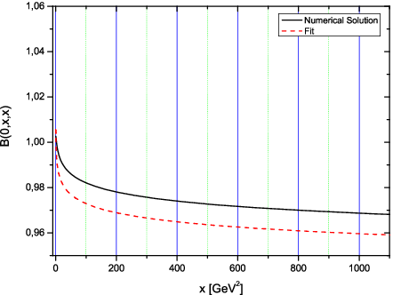
regardless of the form of momentum dependence employed for . Evidently, for large values of the above expression goes over the asymptotic solution of Eq.(3.12). In Figs.(5), we present a typical solution for together with the fit given by (3.20).
IV Infrared finite ghost propagator
In the previous section we have obtained the general solutions for , under the assumption that the ghost propagator was finite in the IR, and more specifically that it was given by the general form of (3.16). The next crucial step consists in substituting the solutions obtained for into (2.10) and in examining under what conditions the two hand sides of the equation can be made to be equal. As we will see this procedure will eventually boil down to constraints on the values that one is allowed to choose for the free parameter .
Substituting Eqs.(3.16) and (3.20) into (2.10), we arrive at
| (4.21) |
The r.h.s. of (4.21) is simply given by
| (4.22) |
for any form of . Let us first verify the self-consistency of (4.21) for the case where the ghost mass vanishes identically, i.e. . Then, (4.21) reduces to nothing but the standard dimensional regularization result Collins
| (4.23) |
valid for any value of , for the special value .
For non-vanishing the integral on the r.h.s. of (4.21) is UV divergent: at large it goes as , where is a UV momentum cutoff. It turns out that the r.h.s. can be made UV finite by simply subtracting from it its perturbative value, i.e. the vanishing integral of (4.23) foot2.
Carrying out this regularization procedure explicitly, one obtains
| (4.24) | |||||
It is now elementary to verify that the integral on the r.h.s of (4.24) converges. At large we can expand the second term in the parenthesis and neglecting in the denominator next to , we find that the resulting integral (apart of multiplicative factors) is given by
| (4.25) |
Notice that the above integral converges even for the less favorable case of a constant ; then, (4.25) is proportional to , and is therefore convergent, since . Clearly, when drops off in the UV, as described by (3.18) or (3.19), the integral converges even faster. Next we will analyze separately what happens for each one of the three different Ansätze we have employed for , Eqs.(3.17) – (3.19).
The case of a constant ghost mass can be easily worked out. Replacing in Eq.(4.24), keeping only the leading contribution to the integral, we arrive at (notice the cancellation of the coupling constant appearing in front of the integral)
| (4.26) |
Then, in order to enforce the equality of both sides of (4.26) must satisfy
| (4.27) |
Evidently, depends very weakly on , and its value is practically fixed at . Indeed, given that is a small number, of the order of , Eq.(4.27) may be expanded as
| (4.28) |
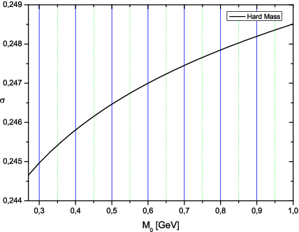
from where it is clear that can only assume values slightly different of . In Fig.(6), we show this mild dependence of on , for .
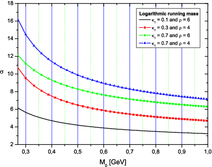
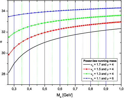
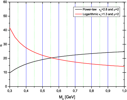
We next turn to the case where displays the logarithmic or power-law dependence on the momentum, described by Eqs. (3.18) and (3.19), respectively. Now the integrals cannot be carried out analytically and have been computed numerically. Choosing different values for , , and , we obtain the curves presented in Fig.(7) and Fig.(8), showing the dependence of on .
Several observations are in order:
(i) For both types of running the results show a stronger dependence on than in the case of the hard mass.
(ii) The range of possible values for increases significantly. Whereas in the case of constant mass one was practically restricted to a unique value for , namely [viz. Fig.(6)], now one may obtain self-consistent solutions choosing values for over a much wider interval.
(iii) There is a qualitative difference between the logarithmic and power-law running: in the former case is a decreasing function of , while in the latter it is increasing. This offers the particularly interesting possibility of finding values for that furnish self-consistent solutions for either types of running of . A characteristic example where Eq.(4.24) is satisfied for the same value of for both types of running is shown in Fig.(9): for one may generate a ghost mass of , assuming for either the logarithmic running of Eq.(3.18), or the power-law running of Eq.(3.19).
V Discussion and Conclusions
In this article we have demonstrated that it is possible to obtain from the SDEs of QCD an IR finite ghost propagator in the Feynman gauge. In this construction the longitudinal component of the gluon-ghost vertex, which is inert in the Landau gauge, assumes a central role, allowing for to be finite. This is accomplished without having to assume any special properties of the form-factor, other than a nonvanishing limit in the IR; in particular, we do not need to impose the presence of massless poles of the type .
Our procedure may be summarized as follows. First of all, since we are interested in the possibility of obtaining we have focused on the form of the ghost gap equation in the limit of vanishing external momentum, . Next we have linearized the SDE for the form-factor , and have looked for solutions for the special kinematic configuration of vanishing ghost momentum, , which is relevant for the ghost gap equation. The solution may be fitted in the entire range of momenta with a particularly simple, physically motivated expression. Coupling the two equations together, we have obtained the conditions necessary for self-consistency. It essentially boils down to relations between the free parameter and the values of , or equivalently , as captured in Figs (6)–(8). These figures furnish the value of one obtains if a concrete value of is chosen, assuming certain characteristic types of running for the the ghost mass function . The freedom in choosing the value of will be restricted, or completely eliminated, in the non-linear version of the vertex equation. It would certainly be interesting to venture into such a study, because it is liable to pin down completely the value of .
The most immediate physical implication of the results presented here is that the finite gluon propagator obtained in the previous SDE studies in the PT-BFM framework, with the ghost contributions gauge-invariantly omitted, will not get destabilized by the inclusion of the ghost loops. Specifically, one would expect that the addition of the ghost loop into the corresponding SDE should not change the qualitative picture. The quantitative changes induced should also be small; mainly the correct coefficient of multiplying the renormalization group logarithms will be restored (without the ghosts it is ), and it might inflate or deflate slightly the corresponding solutions for the gluon propagator in the intermediate region between . Of course, a complete analysis of the coupled SDE system is needed in order to fully corroborate this general picture.
Given the complexity and importance of the problem at hand it would certainly be essential to confront these SDE results with lattice simulations of the ghost propagator in the Feynman gauge. In addition, since the formulation of the BFM on the lattice has been presented long ago by Dashen and Gross (in the Feynman gauge) Dashen:1980vm, and has already been used DiGiacomo:1987tf; Trottier:1997bn, one might also consider the possibility of simulating the gluon propagator within that particular gauge-fixing scheme, thus enabling a direct comparison with the SDE results predicting an IR finite answer.
Acknowledgments
This work was supported by the Spanish MEC under the grants FPA 2005-01678 and FPA 2005-00711. The research of JP is funded by the Fundación General of the UV.
References
- (1) M. Creutz, Phys. Rev. D 21 (1980) 2308.
- (2) J. E. Mandula and M. Ogilvie, Phys. Lett. B 185 (1987) 127.
- (3) C. W. Bernard, C. Parrinello and A. Soni, Phys. Rev. D 49, 1585 (1994) [arXiv:hep-lat/9307001].
- (4) F. J. Dyson, Phys. Rev. 75, 1736 (1949).
- (5) J. S. Schwinger, Proc. Nat. Acad. Sci. 37, 452 (1951); Proc. Nat. Acad. Sci. 37, 455 (1951).
- (6) J. M. Cornwall, R. Jackiw and E. Tomboulis, Phys. Rev. D 10, 2428 (1974).
- (7) W. J. Marciano and H. Pagels, Phys. Rept. 36, 137 (1978).
- (8) C. Becchi, A. Rouet and R. Stora, Annals Phys. 98, 287 (1976); I. V. Tyutin, LEBEDEV-75-39;
- (9) D. Binosi and J. Papavassiliou, Phys. Rev. D 66, 111901 (2002); J. Phys. G 30, 203 (2004); JHEP 0703, 041 (2007).
- (10) J. M. Cornwall, Phys. Rev. D 26 (1982) 1453.
- (11) J. M. Cornwall and J. Papavassiliou, Phys. Rev. D 40, 3474 (1989).
- (12) L. F. Abbott, Nucl. Phys. B 185, 189 (1981).
- (13) A. C. Aguilar and J. Papavassiliou, JHEP 0612, 012 (2006).
- (14) A. C. Aguilar and J. Papavassiliou, arXiv:0708.4320 [hep-ph].
- (15) J. M. Cornwall, Nucl. Phys. B 157, 392 (1979).
- (16) C. W. Bernard, Phys. Lett. B 108, 431 (1982); C. W. Bernard, Nucl. Phys. B 219, 341 (1983); J. F. Donoghue, Phys. Rev. D 29, 2559 (1984).
- (17) For an extended list of references see Aguilar:2006gr.
- (18) C. Alexandrou, P. de Forcrand and E. Follana, Phys. Rev. D 63, 094504 (2001); Phys. Rev. D 65, 117502 (2002); Phys. Rev. D 65, 114508 (2002); P. O. Bowman, U. M. Heller, D. B. Leinweber, M. B. Parappilly and A. G. Williams, Phys. Rev. D 70, 034509 (2004); F. D. R. Bonnet, P. O. Bowman, D. B. Leinweber, A. G. Williams and J. M. Zanotti, Phys. Rev. D 64, 034501 (2001).
- (19) A. Cucchieri and T. Mendes, arXiv:0710.0412 [hep-lat]; I. L. Bogolubsky, E. M. Ilgenfritz, M. Muller-Preussker and A. Sternbeck, arXiv:0710.1968 [hep-lat]; P. O. Bowman et al., arXiv:hep-lat/0703022.
- (20) P. Pascual and R. Tarrach, Nucl. Phys. B 174, 123 (1980) [Erratum-ibid. B 181, 546 (1981)].
- (21) This is a reasonable assumption, and in the conventional formulation (covariant gauges) is valid to all-orders in perturbation theory, given that one may set directly when calculating Feynman diagrams; this is so because the dependence on enters exclusively through the bare propagators, which furnish positive powers of . Since the Feynman rules relevant for the ghost sector are common to both the covariant gauges and the BFM (all fields involved are “quantum” fields) this is also true in our case. Notice however that this is not true in general in the BFM. For instance, since the bare three- and four-gluon vertices involving background and quantum gluons contain terms that go as , background Green’s functions in the Landau gauge must be computed with particular care, taking the limit only after implementing a series of cancellations.
- (22) C. S. Fischer, J. Phys. G 32, R253 (2006) [arXiv:hep-ph/0605173].
- (23) Ph. Boucaud et al., Eur. Phys. J. A 31, 750 (2007); Ph. Boucaud et al., JHEP 0606, 001 (2006).
- (24) A. Cucchieri, T. Mendes and A. Mihara, JHEP 0412, 012 (2004)
- (25) W. Schleifenbaum, A. Maas, J. Wambach and R. Alkofer, Phys. Rev. D 72, 014017 (2005)
- (26) P. Watson, arXiv:hep-ph/9901454; A. I. Davydychev, P. Osland and O. V. Tarasov, Phys. Rev. D 58, 036007 (1998); Phys. Rev. D 54, 4087 (1996) [Erratum-ibid. D 59, 109901 (1999)].
- (27) D. Dudal, N. Vandersickel and H. Verschelde, Phys. Rev. D 76, 025006 (2007) [arXiv:0705.0871 [hep-th]]; D. Dudal, S. P. Sorella, N. Vandersickel and H. Verschelde, arXiv:0711.4496 [hep-th].
- (28) A. C. Aguilar, A. A. Natale and P. S. Rodrigues da Silva, Phys. Rev. Lett. 90, 152001 (2003); A. C. Aguilar, A. Mihara and A. A. Natale, Phys. Rev. D 65, 054011 (2002); Int. J. Mod. Phys. A 19 (2004) 249.
- (29) See, Eq.(4.2.6) in J.C.Collins, “Renormalization”, Cambrigde University Press, Cambridge, 1984.
- (30)
This is a rather standard operation in dimensional regularization.
Its most familiar version is nothing but the usual statement that
in dimensional regularization there are no quadratic divergences,
simply because ,
and therefore
- (31) R. F. Dashen and D. J. Gross, Phys. Rev. D 23, 2340 (1981).
- (32) A. Di Giacomo, M. Maggiore and H. Panagopoulos, Phys. Rev. D 36, 2563 (1987).
- (33) H. D. Trottier and G. P. Lepage, Nucl. Phys. Proc. Suppl. 63, 865 (1998).