Motivated by Schnabl’s gauge choice, we explore open string perturbation theory in gauges where a linear combination of antighost oscillators annihilates the string field. We find that in these linear $b$ -gauges different gauge conditions are needed at different ghost numbers. We derive the full propagator and prove the formal properties which guarantee that the Feynman diagrams reproduce the correct on-shell amplitudes. We find that these properties can fail due to the need to regularize the propagator, and identify a large class of linear $b$ -gauges for which they hold rigorously. In these gauges the propagator has a non-anomalous Schwinger representation and builds Riemann surfaces by adding strip-like domains. Projector-based gauges, like Schnabl’s, are not in this class of gauges but we construct a family of regular linear $b$ -gauges which interpolate between Siegel gauge and Schnabl gauge.

1 Introduction and summary

Since the discovery of interacting open bosonic string field theory [1], much work has been devoted to understanding the Feynman rules of the theory and deriving the Polyakov amplitudes using these Feynman rules [2, 3, 4, 5]. Most of these studies have been carried out in the Siegel gauge [6]. More recently, Schnabl’s discovery [7] of an analytic classical solution in string field theory in a different gauge has inspired a large amount of work on open string field theory in Schnabl gauge and closely related gauges. Most of these studies focus on finding classical solutions of open string field theory and/or studying various properties of these solutions [8, 9, 10, 11, 12, 13, 14, 15, 16, 17, 18, 19, 20, 21, 22, 23, 24, 25, 26, 27, 28, 29].

There has also been some progress towards obtaining the Feynman rules of string field theory in this new class of gauges and computing off-shell amplitudes [30, 31] (see also [32]). The off-shell Veneziano amplitude in Schnabl gauge was obtained in [31], completing the work of [30]. There was a surprise. The amplitude receives contributions from terms whose Siegel gauge analogs would vanish. These contributions require delicate regularization of the propagator which makes the construction of general tree amplitudes quite nontrivial. Motivated by this puzzle in this paper we carry out a systematic study of string perturbation theory in a wide class of gauges which we shall call ‘linear $b$ -gauges’. These gauges include both Siegel gauge and Schnabl gauge as special cases. Other special cases of such gauges have been studied previously in [33].

Our analysis demystifies some of the results found in [31]. We find that the delicate contributions which arise at tree level occur because the propagator fails to move the open string midpoint. Moreover, we show that what has so far been called the Schnabl-gauge propagator is the correct propagator only at the string tree level. For string loop diagrams we need to include string fields of all ghost numbers [4, 5], and the propagator takes different form in different ghost-number sectors. This is a general feature of linear $b$ -gauges. Even after taking this effect into account the proof of consistency of Feynman amplitudes is complicated in Schnabl gauge, again because the propagator does not move the open string midpoint. Motivated by this observation we derive a set of conditions which guarantee that a linear $b$ -gauge defines a consistent perturbation theory. This is one of our main results. Schnabl gauge fails to satisfy these conditions.¹¹ 1 Since our conditions are sufficient but not necessary for a gauge choice to be valid, the failure of the Schnabl gauge to satisfy our condition does not immediately rule it out as a valid gauge choice. It shows, however, that establishing consistency of string perturbation theory in Schnabl gauge is a much more difficult task. During the course of our analysis we obtain an interesting and explicit Riemann surface interpretation of the propagator for general linear $b$ -gauges. We also construct a family of regular linear $b$ -gauges which interpolate between Schnabl gauge and Siegel gauge.

We shall now summarize the main results of the paper. As is well known, a general quantum string field $|\psi\rangle$ is described by a state in the first quantized open string state space with arbitrary ghost number. After suitable gauge fixing the action takes the form:

S=-\left[{1\over 2}\langle\psi|Q|\psi\rangle+{g_{o}\over 3}\langle\psi|\psi*\psi\rangle\right]\,.

(1.1)

Here $Q$ denotes the BRST operator, $*$ denotes star product, and $g_{o}$ is the open string coupling constant. This form of the action may be obtained either by starting with the classical string field theory (which has the same action but $|\psi\rangle$ restricted to ghost-number one) and going through the Fadeev-Popov procedure or by using the Batalin-Vilkovisky formalism. We choose the gauge condition on the ghost-number $g$ string field $|\psi_{(g)}\rangle$ as

{\cal B}_{(g)}|\psi_{(g)}\rangle=0\,,

(1.2)

where ${\cal B}_{(g)}$ is a linear combination of the oscillators $b_{n}$ that can be encoded in a vector field $v(\xi)$ :²² 2 At this point we regard the vector field $v(\xi)$ as a formal Laurent series in $\xi$ . Later we will demand that this Laurent series defines an analytic function in some neighborhood of the unit circle $|\xi|=1$ .

{\cal B}_{(g)}\equiv\sum_{n\in\mathbb{Z}}v_{n}b_{n}=\oint{d\xi\over 2\pi i}\,v(\xi)b(\xi)\,,\qquad\hbox{with}\quad v(\xi)=\sum_{n\in\mathbb{Z}}v_{n}\xi^{n+1}\,.

(1.3)

For each ghost-number $g$ we need a vector field to define the operator ${\cal B}_{(g)}$ . We find that the consistency of gauge fixing requires us to choose

\boxed{\phantom{\Bigl(}\,\,{\cal B}_{(3-g)}={\cal B}_{(g)}^{\star}\,,~}

(1.4)

where ${\cal B}_{(g)}^{\star}$ denotes the BPZ conjugate of ${\cal B}_{(g)}$ . We shall refer to this as a linear $b$ -gauge. Siegel gauge corresponds to the choice ${\cal B}_{(g)}=b_{0}$ for all $g$ . In Schnabl gauge we have

{\cal B}_{(1)}=B\equiv b_{0}+2\sum_{k=1}^{\infty}{(-1)^{k+1}\over 4k^{2}-1}\,b_{2k}\,,\quad v(\xi)=(1+\xi^{2})\tan^{-1}\xi\,.

(1.5)

For a general linear $b$ -gauge ${\cal B}_{(g)}$ is not invariant under BPZ conjugation and eq.(1.4) prevents us from choosing the same gauge condition on all ghost sectors. In particular, Schnabl’s ${\cal B}_{(1)}$ is not BPZ invariant and cannot be used for all ghost numbers. One must have ${\cal B}_{(2)}={\cal B}_{(1)}^{\star}\not={\cal B}_{(1)}$ . A natural possibility consistent with (1.4) is to take

{\cal B}_{(g)}=\begin{cases}{B\quad\,\,\hbox{for $g$ odd,}}\cr{B^{\star}\quad\hbox{for $g$ even.}}\end{cases}\,

(1.6)

Both Siegel gauge and Schnabl gauge are examples in which ${\cal B}_{(g)}$ , for a given $g$ , is a linear combination of $b_{n}$ modes with $n\geq 0$ or with $n\leq 0$ . We will also be able to handle the case of linear combinations of $b_{n}$ modes with both positive and negative $n$ .

It is useful to assemble all the ${\cal B}_{(g)}$ operators into a single operator ${\cal B}$ defined by

{\cal B}=\sum_{g}{\cal B}_{(g)}\Pi_{g}\,,

(1.7)

where $\Pi_{g}$ is the projector onto ghost-number $g$ states. Acting on a ghost-number $g$ state we have ${\cal B}={\cal B}_{(g)}$ , and the gauge-fixing condition (1.2) becomes

{\cal B}|\psi\rangle=0\,.

(1.8)

There are some possible subtleties in defining and manipulating the propagators in a general linear $b$ -gauge, just like in the case of Schnabl gauge [31]. We shall first ignore these subtleties and summarize our results in formal terms and then describe how we address these subtleties. In order to calculate the propagator in the gauge (1.8) we introduce ghost-number $g$ sources $|J_{(g)}\rangle$ , add to the free string field theory action $-{1\over 2}\sum_{g}\langle\psi_{(g)}|Q|\psi_{(2-g)}\rangle$ the source term $\sum_{g}\langle\psi_{(g)}|J_{(3-g)}\rangle$ , and eliminate $|\psi_{(g)}\rangle$ by its linearized equation of motion in the gauge (1.2). The result is ${1\over 2}\sum_{g}\langle J_{(4-g)}|{\cal P}|J_{(g)}\rangle$ , with the full propagator ${\cal P}$ given by

\boxed{\phantom{\Biggl(}{\cal P}=\sum_{g}{\cal P}_{(g)}\Pi_{g}\,,\quad\hbox{with}\quad{\cal P}_{(g)}=\frac{{\cal B}_{(g-1)}}{{\cal L}_{(g-1)}}\,Q\,\frac{{\cal B}_{(g)}}{{\cal L}_{(g)}}\,,\quad\hbox{and}\quad{\cal L}_{(g)}\equiv\{Q,{\cal B}_{(g)}\}\,.~}

(1.9)

Note that at each ghost number the propagator involves the gauge-fixing operators ${\cal B}_{(g)}$ of two ghost numbers. Using (1.9) one can prove the fundamental property

\boxed{\phantom{\Bigl(}~\{Q,{\cal P}\}=1\,.~}

(1.10)

We will show that eq.(1.10) guarantees the decoupling of trivial states from on-shell scattering amplitudes. Moreover, it ensures that the $b$ -gauge propagator $\cal{P}$ gives the same on-shell amplitudes as the familiar Siegel gauge propagator $\overline{\cal P}=b_{0}/L_{0}$ . The steps which lead to this conclusion are straightforward. Since we also have $\{Q,\overline{{\cal P}}\}=1$ , it follows that the difference of propagators $\Delta{\cal P}={\cal P}-\overline{{\cal P}}$ is annihilated by $Q$ , ı.e. $\{Q,\Delta{\cal P}\}=0$ . We find that $\Delta{\cal P}$ is in fact a BRST commutator:

\Delta{\cal P}=[Q,\Omega]\,,

(1.11)

for some operator $\Omega$ . As a result, given any amplitude in the linear $b$ -gauge, we can replace each propagator ${\cal P}$ by $\overline{\cal P}+[Q,\Omega]$ . We show that the contribution from the $[Q,\Omega]$ piece vanishes for on-shell amplitudes after summing over Feynman diagrams. The proof involves the same kind of cancelations which prove that pure-gauge states decouple from on-shell amplitudes in Siegel gauge. The combinatoric factors are somewhat different but they work out correctly.

As anticipated above, not all linear $b$ -gauges are consistent gauge choices. To begin our analysis we make the natural assumption that string field theory Feynman diagrams must have a representation as correlators on Riemann surfaces. The propagator will not permit this representation unless the operators ${\cal L}_{(g)}$ generate conformal transformations of open string theory. This implies that the vector field $v(\xi)$ associated with ${\cal B}_{(g)}$ must satisfy $\overline{v(\xi)}=v(\bar{\xi})$ . We will also see that compatibility with the reality condition on the string field requires vector fields $v(\xi)$ which are even or odd under $\xi\to-\xi$ . Thus a gauge choice which allows real string fields in the gauge slice and which permits a geometric interpretation of ${\cal L}_{(g)}$ requires

\overline{v(\xi)}=v(\bar{\xi})\,,\qquad v(-\xi)=\pm v(\xi)\,.

(1.12)

A rigorous proof of (1.10) gives further constraints. The main obstruction comes from the subtleties in defining the operators $1/{\cal L}_{(g)}$ which appear in the propagator (1.9). We of course do not expect ${\cal L}_{(g)}$ to be invertible in the full space of open string states. First of all it has zero eigenvalues when acting on on-shell states – representatives of BRST cohomology which satisfy the gauge condition. It may also have additional zeroes acting on BRST trivial states satisfying the gauge condition if there are residual gauge symmetries. These are familiar situations which occur even in conventional field theories, and give rise to poles in the propagator at special values of the momentum. What one requires is that ${\cal L}_{(g)}$ should have a well defined inverse acting on states of generic momentum. In particular if we restrict the momentum to the deep Euclidean region (more precisely in the region $k^{2}>1$ so that we avoid the tachyon pole) then the inverse of ${\cal L}_{(g)}$ should be unambiguously defined.

In open string perturbation theory the operator $1/{\cal L}_{(g)}$ appears in the calculation of the string amplitudes. In all linear $b$ -gauges that we consider, amplitudes have a geometric interpretation in terms of Riemann surfaces. We shall see that the requirement on ${\cal L}_{(g)}$ described in the previous paragraph is equivalent to demanding that ${\cal L}_{(g)}$ can be inverted up to terms which represent Riemann surfaces with an open string degeneration, ı.e. surfaces localized at the boundary of the moduli space. Such surfaces contain a strip domain of infinite length. Their contribution vanishes when the momentum flowing along the strip satisfies $k^{2}>1$ because this ensures that only positive conformal weight states propagate along the infinitely long strip.³³ 3 This cannot be done for loop amplitudes where we need to integrate over the internal momentum and we get non-vanishing contributions from the tachyon and massless states propagating in the loop. Only after ignoring these infrared problems, which have a well-defined physical origin, the contributions from degenerate Riemann surfaces can be dropped. In summary, when we demand that for consistent gauge choices $1/{\cal L}_{(g)}$ is well defined and eq.(1.10) is satisfied, we only demand this to hold up to terms whose associated Riemann surfaces are localized at the boundary of the moduli space.

To illustrate this consider first the case of Siegel gauge where the corresponding operator is $1/L_{0}$ . There we define $1/L_{0}$ as

{1\over L_{0}}\equiv\lim_{\Lambda_{0}\to\infty}\int_{0}^{\Lambda_{0}}ds\,e^{-sL_{0}}\,.

(1.13)

A short calculation shows that we have $L_{0}\int_{0}^{\Lambda_{0}}ds\,e^{-sL_{0}}=1-e^{-\Lambda_{0}L_{0}}$ for finite $\Lambda_{0}$ . In a given line of a Feynman diagram the operator $e^{-\Lambda_{0}L_{0}}$ inserts a long strip of width $\pi$ and length $\Lambda_{0}$ into the Riemann surface associated with the amplitude. In the $\Lambda_{0}\to\infty$ limit we get a Riemann surface at the boundary of the moduli space and its contribution can be safely ignored in the sense described above. Thus the relation $L_{0}\int_{0}^{\Lambda_{0}}ds\,e^{-sL_{0}}=1$ becomes exact in the $\Lambda_{0}\to\infty$ limit, leading to the definition (1.13) of $1/L_{0}$ . The analysis for a linear $b$ -gauge is similar. We attempt to define $1/{\cal L}_{(g)}$ for each ghost-number $g$ as

{1\over{\cal L}_{(g)}}\equiv\lim_{\Lambda_{(g)}\to\infty}\int_{0}^{\Lambda_{(g)}}ds\,e^{-s{\cal L}_{(g)}}\,.

(1.14)

For finite $\Lambda_{(g)}$ we have ${\cal L}_{(g)}\int_{0}^{\Lambda_{(g)}}ds\,e^{-s{\cal L}_{(g)}}=1-e^{-\Lambda_{(g)}{\cal L}_{(g)}}$ . It turns out that unless the operators ${\cal L}_{(g)}$ satisfy certain conditions, the $e^{-\Lambda_{(g)}{\cal L}_{(g)}}$ factor can generate contributions away from the boundary of the moduli space even in the $\Lambda_{(g)}\to\infty$ limit and may not be ignored. In this case the Schwinger parametrization (1.14) is anomalous and does not provide a proper inverse to the operator ${\cal L}_{(g)}$ . Contributions to amplitudes which involve factors of $e^{-\Lambda_{(g)}{\cal L}_{(g)}}$ vanish in the limit $\Lambda_{(g)}\to\infty$ if the vector field $v(\xi)$ is analytic in some neighborhood of the unit circle $|\xi|=1$ and satisfies

v_{\perp}(\xi)\equiv\Re\bigl(\bar{\xi}v(\xi)\bigr)>0\quad\hbox{for $|\xi|=1$}\,.

(1.15)

As the notation indicates, $v_{\perp}(\xi)$ is the component of $v(\xi)$ along the radial outgoing direction. The above condition states that on the unit circle $v(\xi)$ never vanishes and always points outward.

Refer to caption — Figure 1: The shape of the strip ${\cal R}(s)$ associated with the operator $e^{-s{\cal L}_{(g)}}$ .

So far we have found that an operator ${\cal B}_{(g)}$ defines a sensible gauge condition if the associated vector field $v(\xi)$ satisfies (1.12) and (1.15). It is easy to see that if $v(-\xi)=v(\xi)$ we cannot satisfy (1.15) both at $\xi$ and $-\bar{\xi}$ . We must require $v(\xi)$ to be odd under $\xi\to-\xi$ . We can then summarize the conditions on $v(\xi)$ which guarantee a regular gauge as follows:

\boxed{\phantom{\Biggl(}v(\xi)=\sum_{k\in\mathbb{Z}}v_{2k}\,\xi^{2k+1}\quad\hbox{with}~v_{2k}\in\mathbb{R}\quad\hbox{and}\quad v_{\perp}(\xi)\equiv\Re\bigl(\bar{\xi}v(\xi)\bigr)>0\quad\hbox{for $|\xi|=1$}\,,~}

(1.16)

with $v(\xi)$ analytic in some neighborhood of the unit circle $|\xi|=1$ . These conditions must be imposed on all the vectors needed to define the ${\cal B}$ operator.⁴⁴ 4 Condition (1.4) does not impose further constraints on the vector field $v(\xi)$ because the BPZ dual vector field $v^{\star}(\xi)$ satisfies (1.16) whenever $v$ does. For $v(\xi)$ satisfying (1.16) in every ghost number sector, eqs.(1.10) and (1.11) hold strictly and lead to rigorous proofs of the decoupling of pure gauge states and the equality of on-shell amplitudes in linear $b$ -gauges and Siegel gauge. Therefore a gauge choice that satisfies (1.16) will be called a regular gauge.

We would like to emphasize that these conditions, while sufficient for the gauge choice to be consistent, are not necessary. For example, we may get a consistent gauge choice even if $v(\xi)$ vanishes at some point $\xi_{0}$ on the unit circle provided the integral $\int^{\xi}d\xi^{\prime}/v(\xi^{\prime})$ is finite along a contour passing through $\xi_{0}$ (see footnote 14). This integral can only be finite if $v(\xi)$ fails to be analytic at $\xi_{0}$ . We will not consider such gauges in this paper.

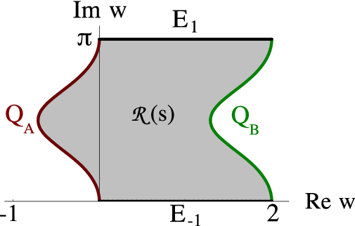
We show that whenever condition (1.16) is satisfied, the insertion of the operator $e^{-s{\cal L}_{(g)}}$ (with $s>0$ ) in a correlation function function can be represented by a strip ${\cal R}(s)$ of length $s$ (see Fig. 1). The coordinate frame for this representation is naturally provided by the Julia equation. The width of the strip ${\cal R}(s)$ is non-vanishing, finite, and independent of $s$ . The strip ${\cal R}(s)$ is bounded above and below by a pair of horizontal lines with open string boundary conditions. Unlike the rectangular strip associated with $e^{-sL_{0}}$ , the left and the right edges of ${\cal R}(s)$ , which are glued to the rest of the Riemann surface, are ragged. In fact they are identically shaped smooth curves of finite horizontal spread. We prove that in the $s\to\infty$ limit the insertion of ${\cal R}(s)$ gives a degenerate Riemann surface – a surface at the boundary of the moduli space. Using this we show that the extra terms which arise in the calculation of amplitudes due to the regularization of $1/{\cal L}_{(g)}$ are localized near the boundary of the moduli space and can be ignored. We also explain geometrically why amplitudes in linear $b$ -gauges other than Siegel gauge cannot exhibit off-shell factorization. This failure of off-shell factorization was investigated in detail in [31] for the Veneziano amplitude in Schnabl gauge. We note, however, that off-shell factorization, while elegant and convenient, is not a physical requirement of amplitudes.

The Schnabl gauge condition (1.5) does not satisfy condition (1.16) because the vector field $v(\xi)$ associated with ${\cal B}_{(1)}=B$ vanishes at the point $\xi=i$ on the unit disk: $v(i)=0$ . We can find a family of regular gauge choices by taking

{\cal B}_{(g)}=\begin{cases}{\,~B^{\lambda}\,\,\,\,~\quad\hbox{for $g$ odd,}}\cr{\left(B^{\lambda}\right)^{\star}\quad\hbox{for $g$ even,}}\end{cases}\,

(1.17)

where

B^{\lambda}\equiv e^{\lambda L_{0}}Be^{-\lambda L_{0}}=b_{0}+2\sum_{k=1}^{\infty}{(-1)^{k+1}\over 4k^{2}-1}\,e^{-2k\lambda}\,b_{2k}\,,\qquad 0<\lambda<\infty\,.

(1.18)

The vector field associated with $B^{\lambda}$ is $v^{\lambda}(\xi)=e^{\lambda}v(e^{-\lambda}\xi)$ , where $v(\xi)$ is the vector associated with $B$ (see (1.5)). For $\lambda>0$ the vector $v^{\lambda}$ satisfies condition (1.16). For $\lambda\to 0$ this gauge approaches Schnabl gauge. On the other hand as $\lambda\to\infty$ this gauge goes over to the Siegel gauge. Thus we have a family of regular gauges which interpolate between Siegel gauge and Schnabl gauge.

2 General linear $b$ -gauges

In this section we shall describe general linear $b$ -gauges and the associated propagators. In §2.1 we explain in detail the linear $b$ -gauge conditions on the string field. §2.2 will be devoted to the computation of the propagator in a general linear $b$ -gauge. In §2.3 we describe some algebraic properties of the propagator which will be useful in §3 for studying amplitudes in string field theory. In §2.4 we analyze the conditions under which a linear $b$ -gauge can be considered a physically reasonable gauge choice. Finally in §2.5 we give some explicit examples of linear $b$ -gauges.

2.1 Gauge conditions, ghosts, and gauge fixed action

The gauge-fixing procedure begins by imposing a gauge condition on the classical open string fields, ı.e. the fields $|\psi_{(1)}\rangle$ at ghost number one. The free string field theory that includes these fields is simply

S_{1}=-{1\over 2}\langle\psi_{(1)}|Q|\psi_{(1)}\rangle\,.

(2.1)

The gauge invariance $\delta_{\epsilon}|\psi_{(1)}\rangle=Q|\epsilon_{(0)}\rangle$ , where $|\epsilon_{(0)}\rangle$ is an arbitrary gauge parameter of ghost number zero, is fixed with the gauge condition:

{\cal B}_{(1)}|\psi_{(1)}\rangle=0\,\,.

(2.2)

The operator ${\cal B}_{(1)}$ above is some particular linear combination of the oscillators $b_{n}$ .

In the Fadeev-Popov (FP) procedure one considers the gauge-fixing functions $F_{i}(\psi)$ , such that $F_{i}(\psi)=0$ are the gauge-fixing conditions, and writes a FP ghost action of the form

S_{FP}\,\sim\,\hat{b}^{i}\,\Bigl(\hat{c}^{\alpha}{\delta\over\delta\epsilon^{\alpha}}\Bigr)\delta_{\epsilon}F_{i}(\psi)\,.

(2.3)

Here $\hat{c}^{\alpha}$ and $\hat{b}^{i}$ are the FP ghosts and FP antighosts respectively, and $\delta_{\epsilon}F_{i}$ is the variation of the gauge fixing functions under infinitesimal gauge transformation with parameters $\epsilon^{i}$ . The FP antighosts are in one-to-one correspondence with the gauge-fixing conditions and the FP ghosts are in one-to-one correspondence with the gauge parameters. Since the gauge transformation parameters in open string field theory are in one-to-one correspondence with ghost-number zero states in the underlying conformal field theory (CFT), it is natural to represent the FP ghost fields by ghost-number zero states $|\psi_{(0)}\rangle$ of the CFT. For gauge conditions of the type (2.2) we can associate the FP antighost fields with ghost-number three states $\langle\tilde{\psi}_{(3)}|$ of the CFT, since the ghost action may then be written as

S_{2}=-\langle\tilde{\psi}_{(3)}|\Bigl(\psi_{(0)}{\delta\over\delta\epsilon_{(0)}}\Bigr){\cal B}_{(1)}\,\delta_{\epsilon}|\psi_{(1)}\rangle=-\langle\tilde{\psi}_{(3)}|\Bigl(\psi_{(0)}{\delta\over\delta\epsilon_{(0)}}\Bigr){\cal B}_{(1)}Q|\epsilon_{(0)}\rangle=-\langle\tilde{\psi}_{(3)}|{\cal B}_{(1)}Q|\psi_{(0)}\rangle\,,

(2.4)

where the minus sign has been included for later convenience. It is natural to absorb the ${\cal B}_{(1)}$ factor into the definition of the bra by setting

\langle\psi_{(2)}|\equiv\langle\tilde{\psi}_{(3)}|{\cal B}_{(1)}\,,

(2.5)

so that we have

S_{2}=-\langle\psi_{(2)}|Q|\psi_{(0)}\rangle\,.

(2.6)

Note that $\langle\psi_{(2)}|$ contains fewer degrees of freedom than $\langle\tilde{\psi}_{(3)}|$ since it is subject to the condition

\langle\psi_{(2)}|{\cal B}_{(1)}=0\quad\to\quad{\cal B}_{(1)}^{\,\star}|\psi_{(2)}\rangle=0\,.

(2.7)

Here ${\cal B}_{(1)}^{\,\star}$ denotes the BPZ conjugate of ${\cal B}_{(1)}$ . In fact the degrees of freedom of $\langle\psi_{(2)}|$ are in one to one correspondence with the gauge-fixing conditions (2.2) since the latter may be expressed as $\langle s|\psi_{(1)}\rangle=0$ for arbitrary ghost-number two states $\langle s|$ satisfying $\langle s|{\cal B}_{(1)}=0$ . Thus $\langle\psi_{(2)}|$ is a more faithful representation of the FP antighost fields than $\langle\tilde{\psi}_{(3)}|$ . Note that the ‘gauge condition’ (2.7) on ghost-number two states was preordained once we chose the gauge condition (2.2) on states of ghost number one.

As is well known, the gauge-fixing procedure does not stop here since the ghost action (2.6) also has gauge invariance. This forces us to include an infinite set of FP ghost fields represented by CFT states of ghost number $\leq 0$ , and an infinite set of FP antighost fields represented by CFT states of ghost number $\geq 2$ [4, 5]. To proceed in a more systematic fashion, it is convenient to introduce the full string field $|\psi\rangle$ which is a sum over the string fields $|\psi_{(g)}\rangle$ of different ghost numbers $g$ :

|\psi\rangle=\sum_{g}|\psi_{(g)}\rangle\,.

(2.8)

Let

{\cal B}_{(g)}|\psi_{(g)}\rangle=0\,,

(2.9)

be the ‘gauge condition’ on $|\psi_{(g)}\rangle$ . So far (2.7) tells us that

{\cal B}_{(2)}={\cal B}_{(1)}^{{}^{\,\star}}\,.

(2.10)

At the next step of gauge fixing, the gauge invariance $\delta_{\epsilon}|\psi_{(0)}\rangle=Q|\epsilon_{(-1)}\rangle$ of (2.6) requires that we impose a gauge condition

{\cal B}_{(0)}|\psi_{(0)}\rangle=0\,.

(2.11)

The choice of ${\cal B}_{(0)}$ is quite arbitrary. We need not choose it equal to ${\cal B}_{(1)}$ or ${\cal B}_{(1)}^{\star}$ ; it can be a new linear combination of $b_{n}$ oscillators. The gauge condition (2.11) leads to an action

S_{3}=-\langle\tilde{\psi}_{(4)}|{\cal B}_{(0)}Q|\psi_{(-1)}\rangle\equiv-\langle\psi_{(3)}|Q|\psi_{(-1)}\rangle\,,\quad\hbox{with}\quad{\cal B}_{(0)}^{\star}|\psi_{(3)}\rangle=0\,.

(2.12)

This stage of gauge fixing has given us

{\cal B}_{(3)}={\cal B}_{(0)}^{\star}\,.

(2.13)

Proceeding this way we can pick a new linear combination of $b_{n}$ oscillators for ${\cal B}_{(g)}$ for all $g\leq 0$ to gauge fix the FP ghosts $|\psi_{(g)}\rangle$ . We then introduce FP ghosts $|\psi_{(g-1)}\rangle$ and associated FP antighosts $\langle\psi_{(3-g)}|$ which satisfy the condition ${\cal B}_{(g)}^{\star}|\psi_{(3-g)}\rangle=0$ . This shows that

\boxed{\phantom{\Bigl(}{\cal B}_{(3-g)}={\cal B}_{(g)}^{\star}\,.~}

(2.14)

This is an important result. Since subspaces at ghost numbers $g$ and $3-g$ are BPZ dual, the gauge-fixing condition can be chosen freely only over “half” the states.

We can rewrite the gauge conditions (2.9) in a compact form by introducing the gauge-fixing operator ${\cal B}$ that acts on the full string field. At each ghost number, ${\cal B}$ is defined to act as the operator that imposes the relevant gauge condition. We have

{\cal B}=\sum_{g}{\cal B}_{(g)}\,\Pi_{g}\,,

(2.15)

where $\Pi_{g}$ is the projector to the space of states of ghost number $g$ . The gauge-fixing condition (2.9) can then be written as ${\cal B}\,|\psi\rangle=0$ since

{\cal B}\,|\psi\rangle=0\quad\Longrightarrow\quad\sum_{g}{\cal B}_{(g)}\Pi_{g}\,\sum_{g^{\prime}}|\psi_{(g^{\prime})}\rangle=\sum_{g}{\cal B}_{(g)}|\psi_{(g)}\rangle=0\quad\Longrightarrow\quad{\cal B}_{(g)}\,|\psi_{(g)}\rangle=0\text{ for all }g\,.

(2.16)

The complete gauge fixed free action is given by

\boxed{\phantom{\Biggl(}S=-{1\over 2}\langle\psi_{(1)}|Q|\psi_{(1)}\rangle-\sum_{g=2}^{\infty}\langle\psi_{(g)}|Q|\psi_{(2-g)}\rangle=-{1\over 2}\sum_{g=-\infty}^{\infty}\langle\psi_{(g)}|Q|\psi_{(2-g)}\rangle=-{1\over 2}\langle\psi|Q|\psi\rangle\,,~}

(2.17)

with the string field $|\psi\rangle$ subject to the gauge condition ${\cal B}|\psi\rangle=0$ .⁵⁵ 5 The equality $\langle\psi_{(g)}|Q|\psi_{(2-g)}\rangle=\langle\psi_{(2-g)}|Q|\psi_{(g)}\rangle$ , used to extend the summation range in (2.17), holds because all string fields are Grassmann odd and $Q^{\star}=-Q$ . As is well known, the interaction term of the gauge fixed action takes the form $-{g_{o}\over 3}\langle\psi|\psi*\psi\rangle$ .

In order to facilitate the computation of the propagator in a general linear $b$ -gauge, we shall now write down the projector that projects onto the gauge slice. For each ghost number $g$ , we introduce a ghost-number one operator ${\cal C}_{(g)}$ such that⁶⁶ 6 If the gauge condition ${\cal B}_{(g)}$ contains a contribution of the form $v_{0}b_{0}$ , we can choose ${\cal C}_{(g)}=v_{0}^{-1}c_{0}$ . As we will see, this is always possible for regular linear $b$ -gauges, as $v_{0}>0$ in this case.

\{\,{\cal B}_{(g)}\,,{\cal C}_{(g)}\,\}=1\,.

(2.18)

This equation implies that

\{\,{\cal B}_{(g)}^{\star}\,,-{\cal C}_{(g)}^{\star}\,\}=1\,.

(2.19)

Since ${\cal B}_{(g)}^{\star}={\cal B}_{(3-g)}$ , this allows us to choose the ${\cal C}_{(g)}$ ’s in such a way that

{\cal C}_{(3-g)}\equiv-{\cal C}_{(g)}^{\star}\,.

(2.20)

The projection operator $\Pi_{S}$ into the gauge slice may now be expressed as

\Pi_{S}=\sum_{g}{\cal B}_{(g)}{\cal C}_{(g)}\,\Pi_{g}\,.

(2.21)

Indeed, as a consequence of (2.18) this gives

\Pi_{S}|\psi_{(g)}\rangle={\cal B}_{(g)}{\cal C}_{(g)}|\psi_{(g)}\rangle=|\psi_{(g)}\rangle\,,

(2.22)

for a string field $|\psi_{(g)}\rangle$ satisfying the gauge condition (2.9). One readily verifies that $\Pi_{S}\Pi_{S}=\Pi_{S}$ . To calculate the BPZ conjugate of $\Pi_{S}$ , we first need to know the BPZ conjugate of the ghost number projector $\Pi_{g}$ . As the inner product of a state of ghost number $g$ with a state of ghost number $g^{\prime}$ is non-vanishing only for $g^{\prime}=3-g$ , we conclude that

\Pi_{g}^{\star}=\Pi_{3-g}\,.

(2.23)

We then have

\bigl({\cal B}_{(g)}{\cal C}_{(g)}\Pi_{g}\bigr)^{\star}=-\Pi_{g}^{\star}\,{\cal C}_{(g)}^{\star}{\cal B}_{(g)}^{\star}={\cal C}_{(3-g)}{\cal B}_{(3-g)}\Pi_{3-g}=\bigl(1-{\cal B}_{(3-g)}{\cal C}_{(3-g)}\bigr)\Pi_{3-g}\,.

(2.24)

Recalling the definition (2.21), we obtain

\boxed{\phantom{\Bigl(}\Pi_{S}^{\star}=1-\Pi_{S}\,.~}

(2.25)

Clearly $\Pi_{S}^{\star}\Pi_{S}^{\star}=\Pi_{S}^{\star}$ , so $\Pi_{S}^{\star}$ is the orthogonal projector.

2.2 The propagator

As a next step, we derive the propagator for the class of gauge conditions discussed in §2.1. To illustrate the procedure, let us briefly review one way of deriving the propagator of the free classical string field theory. We start out by adding a source term to the free classical gauge-fixed action:

S_{1}[\psi\,,J]=-{1\over 2}\langle\psi_{(1)}|Q|\psi_{(1)}\rangle+\langle\psi_{(1)}|J_{(2)}\rangle\,.

(2.26)

Here, the string field $|\psi_{(1)}\rangle$ is subject to the gauge condition ${\cal B}_{(1)}|\psi_{(1)}\rangle=0$ . As usual, sources are arbitrary: they are neither killed by $Q$ nor are they subject to gauge conditions. We can then eliminate the classical string field $|\psi_{(1)}\rangle$ from the action by solving its equation of motion

Q|\psi_{(1)}\rangle=|J_{(2)}\rangle\,.

(2.27)

The solution to this equation for the string field $|\psi_{(1)}\rangle$ which also obeys the gauge condition ${\cal B}_{(1)}|\psi_{(1)}\rangle=0$ is given by

|\psi_{(1)}\rangle=\frac{{\cal B}_{(1)}}{{\cal L}_{(1)}}\,Q\,\frac{{\cal B}^{\star}_{(1)}}{{\cal L}^{\star}_{(1)}}|J_{(2)}\rangle\,,

(2.28)

where ${\cal L}_{(g)}=\{Q,{\cal B}_{(g)}\}$ . In deriving (2.28) we have assumed the existence of the operators $1/{\cal L}_{(1)}$ and $1/{\cal L}_{(1)}^{\star}$ which invert ${\cal L}_{(1)}$ and ${\cal L}_{(1)}^{\star}$ respectively, in the sense described in §1. In §4 we will examine what conditions we have to impose on the gauge choice to be able to rigorously define the operators $1/{\cal L}_{(g)}$ . For now we assume that such a suitable choice of gauge has been made. Plugging (2.28) back into the action (2.26) yields

S_{1}[\psi(J),J\,]={1\over 2}\Bigl\langle J_{(2)}\Bigr|\,\frac{{\cal B}_{(1)}}{{\cal L}_{(1)}}\,Q\,\frac{{\cal B}^{\star}_{(1)}}{{\cal L}^{\star}_{(1)}}\,\Bigl|J_{(2)}\Bigr\rangle\,.

(2.29)

This allows us to identify the propagator in the classical open string field theory as

{\cal P}_{(2)}=\frac{{\cal B}_{(1)}}{{\cal L}_{(1)}}\,Q\,\frac{{\cal B}^{\star}_{(1)}}{{\cal L}^{\star}_{(1)}}=\frac{{\cal B}_{(1)}}{{\cal L}_{(1)}}\,Q\,\frac{{\cal B}_{(2)}}{{\cal L}_{(2)}}\,,

(2.30)

where we have used the result from (2.10) that ${\cal B}_{(1)}^{\star}={\cal B}_{(2)}$ . The subscript in ${\cal P}_{(2)}$ indicates that this propagator naturally acts on the ghost-number two source $|J_{(2)}\rangle$ . A propagator with the same operator structure as ${\cal P}_{(2)}$ in (2.30) first appeared in [33]. For the case of Schnabl gauge, the above propagator was first mentioned in [7] and it was used to calculate the off-shell Veneziano amplitude in [30, 31].

It is now easy to generalize this construction to the complete gauge-fixed free action (2.17). We include sources $|J_{(3-g)}\rangle$ for gauge-fixed string fields $|\psi_{(g)}\rangle$ of all ghost numbers and obtain

S[\psi,\,J\,]=-{1\over 2}\sum_{g=-\infty}^{\infty}\langle\psi_{(g)}|Q|\psi_{(2-g)}\rangle+\sum_{g=-\infty}^{\infty}\langle\psi_{(g)}|{J_{(3-g)}}\rangle\,.

(2.31)

The equation of motion for $|\psi_{(g)}\rangle$ now reads

Q|\psi_{(2-g)}\rangle=|{J_{(3-g)}}\rangle\,.

(2.32)

It is again straightforward to determine the string field $|\psi_{(2-g)}\rangle$ which solves this equation and also satisfies the gauge condition ${\cal B}_{(2-g)}|\psi_{(2-g)}\rangle=0$ . We obtain

|\psi_{(2-g)}\rangle=\frac{{\cal B}_{(2-g)}}{{\cal L}_{(2-g)}}\,Q\,\frac{{\cal B}^{\star}_{(g)}}{{\cal L}^{\star}_{(g)}}|J_{(3-g)}\rangle\,,

(2.33)

or, equivalently,

\langle\psi_{(g)}|=\langle J_{(1+g)}|\frac{{\cal B}_{(2-g)}}{{\cal L}_{(2-g)}}\,Q\,\frac{{\cal B}^{\star}_{(g)}}{{\cal L}^{\star}_{(g)}}\,.

(2.34)

Plugging these results back into (2.31) yields

S[\psi(J),J\,]=\frac{1}{2}\sum_{g=-\infty}^{\infty}\Bigl\langle J_{(1+g)}\Bigr|\frac{{\cal B}_{(2-g)}}{{\cal L}_{(2-g)}}\,Q\,\frac{{\cal B}^{\star}_{(g)}}{{\cal L}^{\star}_{(g)}}\Bigl|{J_{(3-g)}}\Bigr\rangle=\frac{1}{2}\sum_{g=-\infty}^{\infty}\Bigl\langle J_{(4-g)}\Bigr|\frac{{\cal B}_{(g-1)}}{{\cal L}_{(g-1)}}\,Q\,\frac{{\cal B}_{(g)}}{{\cal L}_{(g)}}\Bigl|{J_{(g)}}\Bigr\rangle\,,

(2.35)

where we used (2.14) in obtaining the second equality. We can now identify the propagator ${\cal P}_{(g)}$ acting on the source $|J_{(g)}\rangle$ of ghost number $g$ as

\boxed{\phantom{\Biggl(}{\cal P}_{(g)}=\frac{{\cal B}_{(g-1)}}{{\cal L}_{(g-1)}}\,Q\,\frac{{\cal B}_{(g)}}{{\cal L}_{(g)}}\,.\,}

(2.36)

Alternative expressions obtained by using the BPZ conjugation property (2.14) are

{\cal P}_{(g)}=\,\,\frac{{\cal B}_{(g-1)}}{{\cal L}_{(g-1)}}\,Q\,\frac{{\cal B}^{\star}_{(3-g)}}{{\cal L}^{\star}_{(3-g)}}\,\,=\,\,\frac{{\cal B}^{\star}_{(4-g)}}{{\cal L}^{\star}_{(4-g)}}\,Q\,\frac{{\cal B}_{(g)}}{{\cal L}_{(g)}}\,\,=\,\,\frac{{\cal B}^{\star}_{(4-g)}}{{\cal L}^{\star}_{(4-g)}}\,Q\,\frac{{\cal B}^{\star}_{(3-g)}}{{\cal L}^{\star}_{(3-g)}}\,.

(2.37)

We can simplify notation by combining all sources $|J_{(g)}\rangle$ into a single source

|J\rangle\equiv\sum_{g=-\infty}^{\infty}|J_{(g)}\rangle\,,

(2.38)

just as we did for the gauge-fixed string field $|\psi\rangle$ in (2.8). Let us furthermore define the full propagator ${\cal P}$ as the operator whose action on a subspace of ghost number $g$ is given by ${\cal P}_{(g)}$ , i.e.

\boxed{\phantom{\Biggl(}{\cal P}\equiv\sum_{g=-\infty}^{\infty}{\cal P}_{(g)}\,\Pi_{g}\,.~}

(2.39)

Then the elimination of $|\psi\rangle$ from the free action can be conveniently summarized as

S[\psi,J\,]=-{1\over 2}\langle\psi|Q|\psi\rangle+\langle\psi|J\rangle\quad\to\quad S[\psi(J),J\,]=\frac{1}{2}\,\langle J|{\cal P}|J\rangle\,.

(2.40)

Equations (2.36) and (2.39) give the full propagator ${\cal P}$ for general linear $b$ -gauges. The propagator acts differently on states of different ghost number. This is not surprising, considering that for generic linear $b$ -gauges it is impossible to impose the same gauge condition on states of all ghost numbers.

2.3 Properties of the propagator

Let us now turn to study the algebraic properties of the full propagator. We claim that ${\cal P}$ satisfies the important relation

\boxed{\phantom{\biggl(}\{Q,{\cal P}\}=1\,.\,}

(2.41)

We can prove this property as follows:

	$\displaystyle\{Q,{\cal P}\}\,\Pi_{g}$	$\displaystyle=$	$\displaystyle\left(Q{\cal P}_{(g)}+{\cal P}_{(g+1)}Q\right)\Pi_{g}=\Biggl(Q\,\frac{{\cal B}_{(g-1)}}{{\cal L}_{(g-1)}}\,Q\,\frac{{\cal B}_{(g)}}{{\cal L}_{(g)}}+\frac{{\cal B}_{(g)}}{{\cal L}_{(g)}}\,Q\,\frac{{\cal B}_{(g+1)}}{{\cal L}_{(g+1)}}\,Q\Biggr)\Pi_{g}$		(2.42)
		$\displaystyle=$	$\displaystyle\Biggl(Q\,\frac{{\cal B}_{(g)}}{{\cal L}_{(g)}}+\frac{{\cal B}_{(g)}}{{\cal L}_{(g)}}\,Q\Biggr)\Pi_{g}=\Pi_{g}\,.$		(2.42)

Here we have again assumed that the operator $1/{\cal L}_{(g)}$ can be defined rigorously in the sense described in §1 for the linear $b$ -gauge under consideration. Equation (2.42) shows that $\{Q,{\cal P}\}=1$ holds on all subspaces of fixed ghost number $g$ , and it thus holds in general. Notice that ${\cal P}_{(g)}$ , regarded as an operator acting on states of arbitrary ghost number, generically does not satisfy the same property:

\{Q,{\cal P}_{(g)}\}=Q\,\frac{{\cal B}_{(g)}}{{\cal L}_{(g)}}+\frac{{\cal B}_{(g-1)}}{{\cal L}_{(g-1)}}\,Q\neq 1\qquad\text{ if }\quad{\cal B}_{(g)}\neq{\cal B}_{(g-1)}\,.

(2.43)

It is precisely the property (2.41) which will allow us to prove the decoupling of pure-gauge states and the correctness of on-shell amplitudes in §3.

The propagator ${\cal P}$ is BPZ-invariant,

\boxed{\phantom{\Bigl(}{\cal P}^{\star}={\cal P}\,.~}

(2.44)

Indeed, using (2.14) and (2.23) we obtain

\bigl({\cal P}_{(g)}\,\Pi_{g}\bigr)^{\star}=\Pi_{g}^{\star}\,\frac{{\cal B}^{\star}_{(g)}}{{\cal L}^{\star}_{(g)}}\,Q\,\frac{{\cal B}^{\star}_{(g-1)}}{{\cal L}^{\star}_{(g-1)}}=\Pi_{3-g}\,\frac{{\cal B}_{(3-g)}}{{\cal L}_{(3-g)}}\,Q\,\frac{{\cal B}_{(4-g)}}{{\cal L}_{(4-g)}}=\frac{{\cal B}_{(3-g)}}{{\cal L}_{(3-g)}}\,Q\,\frac{{\cal B}_{(4-g)}}{{\cal L}_{(4-g)}}\,\Pi_{4-g}\,.

(2.45)

Recalling the definition (2.39) of the propagator, this establishes ${\cal P}^{\star}={\cal P}$ .

In addition, the propagator satisfies a set of simple properties related to the projection operator $\Pi_{S}$ to the gauge slice:

\Pi_{S}\,{\cal P}={\cal P}\,\Pi_{S}^{\star}={\cal P},\qquad\Pi_{S}^{\star}\,{\cal P}={\cal P}\,\Pi_{S}=0\,.

(2.46)

These equations are readily checked acting on subspaces of fixed ghost number, using the definitions of ${\cal P}_{(g)}$ and $\Pi_{S}$ , and eq.(2.25).

It is convenient to introduce the gauge-fixed kinetic operator $\cal{K}$ , given by

{\cal K}\equiv\Pi_{S}^{\star}\,Q\,\Pi_{S}\,,\qquad{\cal K}^{\star}=-{\cal K}\,.

(2.47)

Using this and $\{Q,{\cal P}\}=1$ we then find

\begin{split}{\cal P}\,{\cal K}={\cal P}\,\Pi_{S}^{\star}\,Q\,\Pi_{S}={\cal P}\,Q\,\Pi_{S}=(1-Q\,{\cal P})\,\Pi_{S}=\Pi_{S}\,.\end{split}

(2.48)

This and the BPZ conjugate relation are

\boxed{\phantom{\Bigl(}{\cal P}\,{\cal K}=\Pi_{S}\,,\quad{\cal K}\,{\cal P}=\Pi_{S}^{\star}\,.~}

(2.49)

This shows that, as expected, the propagator inverts the gauge-fixed kinetic operator on the gauge slice.

2.4 Constraints on linear $b$ -gauges

So far in our analysis we have not imposed any restriction on the linear combinations of $b_{n}$ oscillators which define the operators ${\cal B}_{(g)}$ . The vector field $v(\xi)$ associated with any of the operators ${\cal B}_{(g)}$ through the relations

{\cal B}_{(g)}=\int{d\xi\over 2\pi i}\,v(\xi)b(\xi)=\sum_{n}v_{n}b_{n}\,,\qquad v(\xi)=\sum_{n}v_{n}\xi^{n+1}\,,

(2.50)

was taken to be completely arbitrary. In this subsection we will examine what constraints we need to impose on the coefficients $v_{n}$ to obtain a physically reasonable gauge choice.

First of all, in order to facilitate the analysis of string perturbation theory we require that the string field theory Feynman diagrams represent correlation functions on Riemann surfaces. For this we require the validity of the Schwinger representation of the factors of $1/{\cal L}_{(g)}$ in the propagator:

{1\over{\cal L}_{(g)}}=\lim_{\Lambda_{(g)}\to\infty}\int_{0}^{\Lambda_{(g)}}ds\,e^{-s{\cal L}_{(g)}}\,.

(2.51)

Furthermore, the insertion of $e^{-s{\cal L}_{(g)}}$ into a correlation function must represent the insertion of a piece of world sheet to the Riemann surface that represents the rest of the diagram. For this ${\cal L}_{(g)}$ must generate a conformal transformation. In open string theory a conformal transformation $\delta\xi\propto\,v(\xi)$ is generated by

\int_{C}\left({d\xi\over 2\pi i}\,v(\xi)\,T(\xi)+{d\bar{\xi}\over 2\pi i}\,\,\overline{v(\xi)}\,\,\overline{T(\xi)}\right)\,,

(2.52)

where $C$ denotes the unit semicircle in the upper-half plane and bars indicate complex conjugation. Replacing $v(\xi)$ by $\xi^{n+1}$ we get the generators of conformal transformation:

L_{n}=\int_{C}\left({d\xi\over 2\pi i}\xi^{n+1}\,T(\xi)+{d\bar{\xi}\over 2\pi i}\bar{\xi}^{n+1}\,\overline{T(\xi)}\right)\,.

(2.53)

This gives

{\cal L}_{(g)}=\sum_{n}v_{n}L_{n}=\int_{C}\left({d\xi\over 2\pi i}v(\xi)T(\xi)+{d\bar{\xi}\over 2\pi i}v(\bar{\xi})\,\overline{T(\xi)}\right)\,.

(2.54)

This does not have the form of the generator (2.52) unless

\overline{v(\xi)}=v(\bar{\xi})\,.

(2.55)

Thus, in order that the Feynman diagrams generated by open string field theory have a direct Riemann surface interpretation we must require that the coefficients $v_{n}$ be real,⁷⁷ 7 We can try to define the results for complex $v_{n}$ by analytic continuation of the real $v_{n}$ results. This trick was used in [33] to discuss the gauge condition $(b_{1}+b_{-1})|\psi\rangle=0$ . We shall not consider this possibility here. ı.e. $v(\xi)$ to be real on the real axis.

Even when (2.55) holds and the insertion of $e^{-s{\cal L}_{(g)}}$ has a Riemann surface interpretation, eq. (2.51) may fail to provide the correct definition of $1/{\cal L}_{(g)}$ due to a non-vanishing contribution from the upper limit of integration. This requirement will be analyzed in detail in section §4. It leads to condition (1.15) which requires the vector field $v(\xi)$ to be analytic in some neighborhood of the unit circle $|\xi|=1$ and to satisfy

v_{\perp}(\xi)\equiv\Re\bigl(\bar{\xi}v(\xi)\bigr)>0\quad\hbox{for $|\xi|=1$}\,.

(2.56)

Secondly, in order that the open string field theory action is real, describing a unitary quantum theory, the string field and the interaction vertices must satisfy certain reality conditions. The reality condition on the string field is easily stated [34]: the combined operations of BPZ conjugation and hermitian conjugation (HC) – called star conjugation – must leave the string field invariant. In open string field theory the interaction term must also be real. If the string field is real, the interaction term is real once the coordinate systems around the punctures on the Riemann surface associated with the interaction vertex satisfy a reality condition. The interaction vertex of Witten’s open string field theory satisfies this condition.

Therefore, when we impose linear $b$ -gauge conditions we must make sure that this can be done consistently with the constraint of real string fields. Since the total effect of BPZ followed by HC does not change the ghost number, we can analyze the condition on string fields of fixed ghost number. Consider the gauge condition ${\cal B}_{(g)}|\psi_{(g)}\rangle=0$ , with ${\cal B}_{(g)}$ related to a vector field $v(\xi)$ through the relation (2.50). In order to impose the reality condition we need that if $|\psi_{(g)}\rangle$ satisfies the gauge condition then the star-conjugate of $|\psi_{(g)}\rangle$ automatically satisfies the gauge condition – this allows us to form the linear combination required for reality. For this we must have $({\cal B}_{(g)}^{\star})^{\dagger}\propto{\cal B}_{(g)}$ with $\dagger$ denoting hermitian conjugation. Since the operation of star conjugation is an involution one can only have

({\cal B}_{(g)}^{\star})^{\dagger}=e^{i\alpha}\,{\cal B}_{(g)}\,,

(2.57)

with $\alpha$ real. Recalling that $(b_{n})^{\star}=(-1)^{n}b_{-n}$ and $(b_{n})^{\dagger}=b_{-n}$ , a short calculation shows that

\begin{split}{\cal B}_{(g)}^{\star}&\equiv\int{d\xi\over 2\pi i}\,b(\xi)v^{\star}(\xi)\,,\quad\hbox{with}\quad v^{\star}(\xi)=-\xi^{2}v\bigl(-{1/\xi}\bigr)\\[2.15277pt] {\cal B}_{(g)}^{\dagger}&\equiv\int{d\xi\over 2\pi i}\,b(\xi)v^{\dagger}(\xi)\,,\quad\hbox{with}\quad v^{\dagger}(\xi)=\xi^{2}\,\overline{v\bigl({1/\bar{\xi}}\,\bigr)}\,.\end{split}

(2.58)

Thus (2.57) holds if $(v^{\star})^{\dagger}=e^{i\alpha}v$ . Since

(v^{\star}(\xi))^{\dagger}=\bigl(-\xi^{2}v(-1/\xi)\bigr)^{\dagger}=\xi^{2}\overline{\bigl(-{\bar{\xi}}^{-2}\,v(-\bar{\xi})\bigr)}=-\,\,\overline{v(-\bar{\xi})}\,,

(2.59)

we can rewrite the condition on $v(\xi)$ as

\,e^{i\alpha}v(\xi)=-\,\,\overline{\phantom{a^{a^{2}}}\hskip-12.0ptv(-\bar{\xi})}\,,\quad\hbox{for some real $\alpha$}\,.

(2.60)

Recalling that we required $v(\xi)$ to be real on the real axis, only $e^{i\alpha}=\mp 1$ are allowed in (2.60). Combining this with the condition (2.55) we conclude that the vector field $v$ has to be either even or odd under $\xi\to-\xi$ :

v(-\xi)=\pm\,v(\xi)\,.

(2.61)

It is easy to see that the choice $v(-\xi)=v(\xi)$ is not compatible with conditions (2.55) and (2.56). To prove this assume that condition (2.56) is satisfied for some $\xi$ on the upper-half unit circle:

\Re\bigl(\bar{\xi}\,v(\xi)\bigr)>0\,.

(2.62)

Using (2.55) and $v(-\xi)=v(\xi)$ , it immediately follows that

\Re\bigl(\overline{(-\bar{\xi})}v(-\bar{\xi})\bigr)=\Re\bigl((-\bar{\xi})\overline{v(-\bar{\xi})}\bigr)=\Re\bigl((-\bar{\xi})v(-\xi)\bigr)=-\Re\bigl(\bar{\xi}v(\xi)\bigr)<0\,,

(2.63)

in contradiction with condition (2.56) for $-\bar{\xi}$ . Thus we conclude that physically reasonable gauges must satisfy

\overline{v(\xi)}=v(\bar{\xi})\,,\quad v(-\xi)=-v(\xi)\,,

(2.64)

and thus

\boxed{\phantom{\Biggl(}v(\xi)=\sum_{k\in\mathbb{Z}}v_{2k}\,\xi^{2k+1}\quad\hbox{with}~v_{2k}\in\mathbb{R}\,.~}

(2.65)

It should be noted that the conditions derived so far are consistent with (2.14) – if $v(\xi)$ satisfies (2.56) and the additional conditions (2.64), so does the dual vector $v^{\star}(\xi)$ . Indeed, on the unit circle

\bar{\xi}v^{\star}(\xi)=-\xi v(-1/\xi)=\xi v(1/\xi)=\xi v(\bar{\xi})=\overline{\bar{\xi}\,v(\xi)}\,.

(2.66)

It follows that $\Re\bigl(\bar{\xi}v^{\star}(\xi)\bigr)=\Re\bigl({\bar{\xi}\,v(\xi)}\bigr)>0$ , as we wanted to show. It is straightforward to show that $v^{\star}(\xi)$ satisfies (2.64).

One can examine the constraint (2.56) more explicitly using the Laurent expansion of the vector $v(\xi)$ . Writing $\xi=e^{i\theta}$ we find

v_{\perp}(e^{i\theta})=v_{0}+\sum_{k\neq 0}v_{2k}\cos(2k\theta)>0\,.

(2.67)

Thus the average of $v_{\perp}(e^{i\theta})$ over $0\leq\theta\leq\pi$ is given by

\frac{1}{\pi}\int_{0}^{\pi}d\theta\,v_{\perp}(e^{i\theta})=v_{0}\,,

(2.68)

leading to the constraint

\boxed{\phantom{\biggl(}~v_{0}>0\,.~}

(2.69)

All operators ${\cal B}_{(g)}$ must contain a component along $b_{0}$ with positive coefficient. It also follows from (2.67) that

v_{0}>\sum_{k\neq 0}|v_{2k}|

(2.70)

is sufficient (but not necessary!) for condition (2.56) to be satisfied. It is useful to check that (2.70) is not satisfied for Schnabl gauge. In this gauge (1.5) tells us that the only nonvanishing coefficients are

v_{0}=1\,,\quad v_{2k}={2(-1)^{k+1}\over 4k^{2}-1}\,,\quad k=1,2,\ldots

(2.71)

A short calculation gives

\sum_{k=1}^{\infty}|v_{2k}|=2\sum_{k=1}^{\infty}{1\over 4k^{2}-1}=1=v_{0}\,,

(2.72)

showing that (2.70) is marginally violated. This failure is in fact related to the vanishing of $v(\xi)$ for $\xi=i$ :

v(\xi)=i\Bigl(v_{0}+\sum_{k=1}^{\infty}v_{2k}(-1)^{k}\Bigr)=i\Bigl(v_{0}-\sum_{k=1}^{\infty}|v_{2k}|\Bigr)=0\,.

(2.73)

The vanishing of the vector at any point on the circle means that the conditions for a regular gauge are not satisfied.

2.5 Examples

To define a specific linear $b$ -gauge, we need to choose a linear combination of oscillators $b_{n}$ for each ${\cal B}_{(g)}$ with $g\leq 1$ . The remaining ${\cal B}_{(g)}$ are then fully determined through the relation (2.14), ${\cal B}_{(3-g)}={\cal B}^{\star}_{(g)}$ . The simplest linear $b$ -gauge is Siegel gauge: ${\cal B}_{(g)}=b_{0}$ . As the Siegel gauge condition is BPZ invariant, we can impose the same condition on string fields of all ghost numbers. Schnabl gauge corresponds to the choice ${\cal B}_{(1)}=B$ for classical string fields, with $B$ defined in (1.5). Geometrically, $B$ can be understood as the zero mode of the antighost in the sliver frame:

B=f^{-1}\circ\oint{dz\over 2\pi i}zb(z)=\oint{d\xi\over 2\pi i}{f(\xi)\over f^{\prime}(\xi)}b(\xi)\,=\oint{d\xi\over 2\pi i}v(\xi)b(\xi)\,,

(2.74)

where $\circ$ denotes a conformal transformation, the sliver frame coordinate $z=f(\xi)$ is given by

f(\xi)=\frac{2}{\pi}\tan^{-1}\xi\,,

(2.75)

and

v(\xi)=\frac{f(\xi)}{f^{\prime}(\xi)}=(1+\xi^{2})\tan^{-1}\xi

(2.76)

is the vector field associated with $B$ . The function $f$ maps the point $\xi=i$ to infinity. This property implies that the sliver, regarded as a surface state with local coordinates on the upper half plane defined through the map $f$ , is a projector. Conversely, any map $f(\xi)$ that sends the point $i$ to infinity can be used to describe a projector. A gauge choice is called a projector gauge if ${\cal B}_{(1)}$ is defined just like the operator $B$ in (2.74), but with $f(\xi)$ describing an arbitrary projector. Thus Schnabl gauge is a projector gauge. For any projector gauge $f(\xi)$ diverges at $\xi=i$ and so does $\ln f(\xi)$ and its derivative $f^{\prime}(\xi)/f(\xi)$ . It follows that the associated vector field $v(\xi)=f(\xi)/f^{\prime}(\xi)$ vanishes at $\xi=i$ and hence fails to satisfy condition (1.15). Thus projector gauges are not regular gauges in the sense described in §1.

There is a natural one-parameter family of regular gauges ${\cal B}_{(1)}=B^{\lambda}$ parameterized by $0<\lambda<\infty$ which interpolates between Siegel and Schnabl gauge. $B^{\lambda}$ is defined by

B^{\lambda}\equiv e^{\lambda L_{0}}\,B\,e^{-\lambda L_{0}}\,,\qquad\text{ with }0<\lambda<\infty\,.

(2.77)

Since $B$ is the sum of $b_{0}$ and a linear combination of $b_{n}$ ’s with $n>0$ , the relation

e^{\lambda L_{0}}\,b_{n}\,e^{-\lambda L_{0}}=e^{-\lambda n}b_{n}\,

(2.78)

ensures that we recover Siegel gauge in the limit $\lambda\to\infty$ :

\lim_{\lambda\to\infty}B^{\lambda}=b_{0}\,,

(2.79)

Schnabl gauge on the other hand is not a regular linear $b$ -gauge and corresponds to $\lambda\to 0$ :

B=\lim_{\lambda\to 0}B^{\lambda}\,.

(2.80)

The operator $B^{\lambda}$ is also the zero mode of the antighost field in a certain conformal frame determined up to a real scaling. To determine such a frame $z=f^{\lambda}(\xi)$ we note that the associated vector field $v^{\lambda}(\xi)$ differs in a simple manner from the sliver vector field $v(\xi)$ of (2.76). If we expand

v(\xi)=\sum_{k\in\mathbb{Z}}v_{2k}\,\xi^{2k+1}\,,

(2.81)

then equation (2.78) tells us that

v^{\lambda}(\xi)=\sum_{k\in\mathbb{Z}}v_{2k}\,e^{-2k\lambda}\xi^{2k+1}=e^{\lambda}\sum_{k\in\mathbb{Z}}v_{2k}\,(e^{-\lambda}\xi)^{2k+1}=e^{\lambda}\,v(e^{-\lambda}\xi)\,.

(2.82)

It is now simple to verify that

f^{\lambda}(\xi)=f(e^{-\lambda}\xi)={2\over\pi}\,\tan^{-1}(e^{-\lambda}\xi)\,,

(2.83)

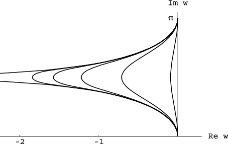
satisfies the expected relation $f^{\lambda}(\xi)/{f^{\lambda}}^{\prime}(\xi)=v^{\lambda}(\xi)$ . For any $\lambda>0$ the coordinate curve $f^{\lambda}(e^{i\theta})$ , $\theta\in[0,\pi]$ is smooth and reaches a maximum finite height for $\theta=\pi/2$ , as shown in Fig. 2.⁸⁸ 8 In (2.83) we chose the normalization $2/\pi$ to reproduce the sliver frame coordinate (2.75) in the limit $\lambda\to 0$ . Alternatively, the normalization $1/\tan^{-1}(e^{-\lambda})$ is convenient to study the Siegel limit $\lambda\to\infty$ , because we have $f^{\lambda}(\xi)=\tan^{-1}(e^{-\lambda}\xi)/\tan^{-1}(e^{-\lambda})=\xi+\mathcal{O}(e^{-\lambda})$ in this case.

The vector field $v^{\lambda}(\xi)$ given in (2.82) satisfies the conditions (1.16). The only nontrivial condition is the one rephrased in (2.67). From (2.82) we see that the expansion coefficients for the vector fields $v^{\lambda}$ and $v$ are related by

v_{2k}^{\lambda}=e^{-2k\lambda}v_{2k}\,,\quad k=0,1,2,\ldots\,.

(2.84)

It then follows that for any $\lambda>0$

\sum_{k=1}^{\infty}|v_{2k}^{\lambda}|<\sum_{k=1}^{\infty}|v_{2k}|=1\,,

(2.85)

after use of (2.72). This shows that the vector $v^{\lambda}$ satisfies (2.70), which suffices for a regular gauge. The $B^{\lambda}$ gauge is not a projector gauge for $\lambda>0$ and does not exhibit the problematic properties of Schnabl gauge. The $\lambda$ parameter allows us to interpolate between Schnabl and Siegel gauge. It may also allow us to regularize and define amplitudes in Schnabl gauge as the limit $\lambda\to 0$ of amplitudes in the $B^{\lambda}$ gauge.

Neither Schnabl gauge nor the $B^{\lambda}$ gauges impose a BPZ invariant gauge condition on the classical string field $|\psi_{(1)}\rangle$ . There is therefore no preferred choice of gauge conditions on the ghost sector string fields. Let us discuss one possible assignment of gauge conditions which we will call alternating gauge. In alternating gauge, we apply the classical gauge condition ${\cal B}_{(1)}|\psi_{(1)}\rangle=0$ to all string fields of odd ghost number $g$ ,

{\cal B}_{(1)}|\psi_{(g)}\rangle=0\qquad\text{for $g$ odd}\,.

(2.86)

This exhausts our freedom to choose conditions. The relation ${\cal B}_{(3-g)}={\cal B}^{\star}_{(g)}$ forces us to assign the BPZ conjugate condition on string fields of even ghost number $g$ :

{\cal B}_{(1)}^{\star}|\psi_{(g)}\rangle=0\qquad\text{for $g$ even}\,.

(2.87)

Let us denote the projectors onto states of even and odd ghost numbers by $\Pi_{+}$ and $\Pi_{-}$ , respectively. Then we can state the gauge condition as

{\cal B}|\psi\rangle=0\,,\quad\text{ with }\quad{\cal B}\equiv{\cal B}_{(1)}\,\Pi_{-}+{\cal B}_{(1)}^{\star}\,\Pi_{+}\,.

(2.88)

The propagator in alternating gauge is readily seen to be given by

\begin{split}{\cal P}&=\frac{{\cal B}_{(1)}}{{{\cal L}_{(1)}}}\,Q\,\frac{{\cal B}_{(1)}^{\star}}{{\cal L}_{(1)}^{\star}}\,\Pi_{+}+\frac{{\cal B}_{(1)}^{\star}}{{\cal L}_{(1)}^{\star}}\,Q\,\frac{{\cal B}_{(1)}}{{\cal L}_{(1)}}\,\Pi_{-}\,.\end{split}

(2.89)

3 Analysis of on-shell amplitudes

In this section we shall analyze the on-shell amplitudes in a general linear $b$ -gauge. In §3.1 we give a simple proof of the decoupling of pure-gauge states. In §3.2 we prove the equality of on-shell amplitudes in a general linear $b$ -gauge and the Siegel gauge. Since the latter is known to reproduce correctly the Polyakov amplitudes in open string theory, this establishes that the on-shell amplitudes in a linear $b$ -gauge give the correct S-matrix of open string theory. The proofs in this section rely on the validity of the relation

\left\{Q,{\cal P}\right\}=1\,.

(3.1)

In §4 and §5 we will carefully analyze this relation by regularizing the operators $1/{{\cal L}_{(g)}}$ that enter in the definition of ${\cal P}$ . We will then determine the conditions that we need to impose for all correction terms to be localized at the boundary of open string moduli space in the limit when we remove the regularization. We will find that (3.1) can be made rigorous for gauge choices which are regular gauges as defined in §1.

3.1 Decoupling of pure gauge states

Consider an on-shell amplitude where every external state is BRST closed and, furthermore, one of the external states is pure gauge, ı.e. has the form $Q|\chi\rangle$ for some ghost-number zero state $|\chi\rangle$ . In this case we can move the $Q$ through the various propagators and vertices of a Feynman diagram contributing to this amplitude using the relations

$\displaystyle Q^{(1)}\,\|V_{123}\rangle$	$\displaystyle=$	$\displaystyle{}-\left(Q^{(2)}+Q^{(3)}\right)\|V_{123}\rangle\,,$	(3.2)
$\displaystyle\left(Q^{(1)}+Q^{(2)}\right)\,\|V_{123}\rangle$	$\displaystyle=$	$\displaystyle{}-Q^{(3)}\|V_{123}\rangle\,,$	(3.3)
$\displaystyle Q\,{\cal P}$	$\displaystyle=$	$\displaystyle-{\cal P}\,Q+1$	(3.4)
$\displaystyle Q\,{\cal P}+{\cal P}\,Q$	$\displaystyle=$	$\displaystyle 1\,.$	(3.5)

Here $|V_{123}\rangle$ denotes the three string vertex. The diagrammatic representations of these three identities are shown in Figs. 3, 4, 5, and 6. An example of how $Q$ moves through a given diagram has been shown in Fig. 7. In fact there are many different orders in which we can move $Q$ through a given diagram, as shown in Figs.7(a) and 7(b), but the final result is independent of this choice and so for each diagram we make a fixed choice. Eqs.(3.4) and (3.5) show that during the process of moving $Q$ through a propagator we are left with an extra contribution where the propagator is replaced by unity. We label it by a collapsed propagator, ı.e a four point vertex. It is clear from the identities (3.2)-(3.5) and their diagrammatic representations Fig.3-Fig.6 that the BRST operator moves through the diagram until it hits an external state, or until it collapses an internal propagator. The contributions from hitting external states vanish, because the external states are BRST closed. Therefore we are left with the contributions from collapsing propagators. A diagram with $n$ internal propagators gives rise to $n$ such terms. In each term, one internal line of the diagram has collapsed, while all other lines have the original propagator ${\cal P}$ . We now combine contributions from different Feynman diagrams. In this case each diagram with a collapsed propagator arises in two different ways, one where the collapsed propagator appears as a t-channel propagator, and another where it appears as an s-channel propagator (see Fig. 8).⁹⁹ 9 Since in the Riemann surface interpretation of string field theory Feynman diagrams each line is blown up to a strip, the cyclic ordering of the labels $i$ , $j$ , $k$ , $l$ is important. Thus for example if we exchange the labels $i$ and $j$ in the left-most diagram of Fig. 8 then it would be regarded as a different string Feynman diagram. For this reason a diagram with a collapsed $u$ -channel propagator has a different structure and needs to be combined with another diagram carrying a different cyclic ordering of the labels $i$ , $j$ , $k$ , $l$ from the one shown in Fig. 8. When this propagator collapses, the t-channel and s-channel diagrams are indistinguishable, and their contributions cancel because they come with opposite signs – a result familiar from the proof of decoupling of pure gauge states in ordinary Siegel gauge amplitudes. Thus the diagrams with collapsed propagators cancel pairwise. This finishes our proof of decoupling of pure gauge states in on-shell amplitudes.

While the proof itself was straight-forward, it is important to identify the main ingredient of the proof. It is in fact eq.(3.4) that tells us that when $Q$ passes through a propagator it leaves behind a contribution that is unity. Had this been a non-trivial operator in the CFT, the cancellation between the $s$ - and $t$ -channel diagrams of Fig. 8 would not have been possible.

3.2 Proof of equivalence to Siegel gauge amplitudes

Let us denote by

\overline{{\cal P}}={b_{0}\over L_{0}}\,,

(3.6)

the propagator in the Siegel gauge. Then the propagator in a general linear $b$ -gauge is given by

{\cal P}=\overline{{\cal P}}+[\,Q,\,\Omega\,]\,.

(3.7)

where¹⁰¹⁰ 10 In the left definition of (3.8) we could replace $\overline{\cal P}=b_{0}/L_{0}$ by any other operator $\widetilde{B}/\widetilde{L}$ where $\widetilde{B}$ is an appropriate linear combination of the $b_{n}$ ’s and $\widetilde{L}=\{Q,\widetilde{B}\}$ , but we have chosen it to be $b_{0}/L_{0}$ to simplify our formulæ.

\Omega\equiv\overline{\cal P}\,\Delta{\cal P}\,,\qquad\Delta{\cal P}\equiv{\cal P}-\overline{{\cal P}}\,.

(3.8)

Indeed, recalling that $\{Q,{\cal P}\}=\{Q,\overline{{\cal P}}\}=1$ we find

[\,Q,\,\Omega\,]=\{\,Q,\overline{{\cal P}}\,\}\,\Delta{\cal P}-\overline{{\cal P}}\,\{Q,\Delta{\cal P}\,\}=\Delta{\cal P}\,.

(3.9)

While equation (3.7) holds for a large class of linear b-gauges, it can break down when certain conditions on the operators ${\cal B}_{(g)}$ are not fulfilled. We will determine these conditions in §4 and §5. We shall now show that assuming relation (3.7) we can replace all the propagators ${\cal P}$ by the Siegel gauge propagator $\overline{{\cal P}}$ in on shell amplitudes. The proof will use manipulations similar to the ones used in §3.1; however the combinatorics will be somewhat different.

Let us consider Feynman diagrams with $k$ external legs and $n$ internal legs. Since we have only three point vertices, the number $n$ is the same for all the diagrams contributing to an amplitude at any given order. The external lines are always labeled, but we shall also label the internal lines as 1, 2, $\cdots$ $n$ . There are $n!$ ways of doing this, so we sum over all the $n!$ possibilities and divide each diagram by $n!$ . We repeat this for every Feynman diagram contributing to a given amplitude at a given order.

Now we collect all Feynman diagrams contributing to an amplitude and replace ${\cal P}$ by $\overline{{\cal P}}+Q\Omega-\Omega Q$ in propagator number 1 in each of these diagrams. There are two possibilities: (a) the propagator 1 may be irreducible, ı.e. the diagram does not break into two pieces when we cut it, (b) it may be reducible so that the diagram breaks into two pieces when we cut it (see Fig. 9). We first consider the possibility (a). For each diagram of this type, we begin with the $Q\Omega$ term and move the $Q$ through vertices and propagators using the relations (3.2)-(3.5). During the process of moving $Q$ through any of the other $(n-1)$ propagators, we again pick up an extra contribution where the propagator is replaced by unity. As in §3.1, we display this by a collapsed propagator, ı.e a four point vertex, but this time the vertex carries the label of the propagator that collapsed, as in figure 8. Other terms where the $Q$ hits external states vanish since the external states are BRST invariant. But this time, because of the irreducibility of propagator 1, we are left with one more term, $\Omega Q$ , from bringing the $Q$ back to the original propagator $1$ on the other side of $\Omega$ . This term cancels the $-\Omega Q$ term of the commutator. Thus, at the end, the $[Q,\Omega]$ part of propagator 1 in a given Feynman diagram of type (a) reduces to a collection of $(n-1)$ diagrams each of which has the operator $\Omega$ on propagator $1$ , a collapsed propagator in one of the lines $2$ , $\cdots$ $n\,$ , and propagators ${\cal P}$ on all other lines. As before, when we combine the contributions from different Feynman diagrams of type (a), there are pairs of identical diagrams¹¹¹¹ 11 This time we call two diagrams identical only if they have both identical topology and matching labels on the internal propagators (collapsed or otherwise) and external lines. with collapsed s- and t-channel propagators. As collapsed s- and t-channel diagrams differ in sign, they again cancel pairwise.

The analysis of case (b) is similar, the only difference being that $Q$ never comes back to the original propagator at the end of the manipulations. The terms which arise from manipulating the $Q\Omega$ part of the commutator leave behind diagrams with one collapsed propagator on one side of the diagram. The terms which arise from manipulating the $-\Omega Q$ part of the commutator leave behind diagrams with one collapsed propagator on the other side of the diagram. Again, when we combine the contributions from all the Feynman diagrams of type (b), the diagrams involving collapsed propagators cancel pairwise.

We have thus shown that the commutator term $[Q,\Omega]$ in propagator 1 in both cases (a) and (b) does not contribute to the amplitude. Thus for each original Feynman diagram we are left with one diagram, with the Siegel gauge propagator $\overline{{\cal P}}$ on line 1 and the original propagator ${\cal P}$ on all other lines.

We can now repeat the analysis by replacing propagator 2 in each diagram by the right hand side of (3.7). The only difference from the previous analysis is that in each diagram propagator 1 is now the Siegel gauge propagator. This does not affect our argument, however, since the Siegel gauge propagator $\overline{{\cal P}}$ , just like ${\cal P}$ , satisfies the relations (3.4) and (3.5), ı.e.

\{Q,\overline{{\cal P}}\}=1\,.

(3.10)

Thus at the end of this process we are left with a sum of diagrams with propagators 1 and 2 replaced by Siegel gauge propagators. Iterating this procedure, we can replace all propagators by Siegel gauge propagators.

Finally we turn to the external states. If ${\cal B}_{(1)}$ is a linear combination of $b_{n}$ ’s with $n\geq 0$ , as in the case of Schnabl gauge, then it is possible to choose the cohomology elements to be the same as the ones used in the Siegel gauge, ı.e. vertex operators of the form $cV$ where $V$ is a dimension 1 matter primary operator. In general we need to choose different representatives of the BRST cohomology in Siegel gauge and a linear $b$ -gauge. However, since we have already proven decoupling of BRST exact states, we can replace each of the external states in the linear $b$ -gauge by the representative of the corresponding BRST cohomology class in the Siegel gauge without changing the amplitude. This establishes that all on-shell amplitudes in a general linear $b$ -gauge are the same as those in Siegel gauge.

4 Conditions from consistent Schwinger representations of $1/{\cal L}_{(g)}$

The formal manipulations of §2 and §3 require that we have a well-defined inverse of the operator ${\cal L}_{(g)}$ for every $g$ , in the sense described in §1. Indeed $1/{\cal L}_{(g)}$ enters the expression for the propagator and various manipulations involving the propagator, – e.g. in the proof of $\{Q,{\cal P}\}=1$ . In this section we shall investigate under what conditions the matrix elements of $1/{\cal L}_{(g)}$ encountered in the calculation of string field theory amplitudes can be rigorously defined up to terms whose associated Riemann surfaces are localized at the boundary of open string moduli space.

As a warm-up let us recall how regularization works in the Siegel gauge. The propagator $1/L_{0}$ is defined as

{1\over L_{0}}\equiv\lim_{\Lambda_{0}\to\infty}\int_{0}^{\Lambda_{0}}ds\,e^{-sL_{0}}\,.

(4.1)

Using the relation

L_{0}\int_{0}^{\Lambda_{0}}ds\,e^{-sL_{0}}=1-e^{-\Lambda_{0}L_{0}}\,,

(4.2)

we see that in order for $\int_{0}^{\Lambda_{0}}ds\,e^{-sL_{0}}$ to give a proper definition of $1/L_{0}$ for $\Lambda_{0}\to\infty$ , the matrix elements of $e^{-\Lambda_{0}L_{0}}$ must vanish in this limit. Thus we must examine what happens to the amplitudes when the propagator on a line is replaced by the operator $e^{-\Lambda_{0}L_{0}}$ . As is familiar, in the presence of this operator the Feynman graph line represents a strip of length $\Lambda_{0}$ and width $\pi$ . As $\Lambda_{0}\to\infty$ the strip becomes infinitely long and the Riemann surface degenerates. As long as the open strings propagating along this infinitely long strip carry positive conformal weight, this contribution can be safely ignored.

Following the same strategy we try to represent $1/{\cal L}_{(g)}$ as $\int_{0}^{\infty}ds\,e^{-s{\cal L}_{(g)}}$ , and then regulate the upper limit of integration over the Schwinger parameter $s$ using a cutoff $\Lambda_{(g)}$ :

\frac{1}{{\cal L}_{(g)}}\,\equiv\lim_{\Lambda_{(g)}\to\infty}\int_{0}^{\Lambda_{(g)}}ds\,e^{-s{\cal L}_{(g)}}\,.

(4.3)

Now we have

{\cal L}_{(g)}\int_{0}^{\Lambda_{(g)}}ds\,e^{-s{\cal L}_{(g)}}=1-e^{-\Lambda_{(g)}{\cal L}_{(g)}}\,.

(4.4)

Thus in order that (4.3) gives a proper definition of $1/{\cal L}_{(g)}$ we need to ensure that in the $\Lambda_{(g)}\to\infty$ limit the $e^{-\Lambda_{(g)}{\cal L}_{(g)}}$ term on the right hand side of (4.4) has vanishing matrix element between any pair of states which arise in the analysis of the Feynman amplitudes of string field theory. Recalling the analysis in the Siegel gauge, we can easily anticipate that in order to prove the existence of $1/{\cal L}_{(g)}$ , we need to ensure that insertion of an operator $e^{-\Lambda_{(g)}{\cal L}_{(g)}}$ produces degenerate Riemann surfaces in the $\Lambda_{(g)}\to\infty$ limit.

Keeping this in mind, we shall now examine the effect of inserting an operator of the form $e^{-s{\cal L}_{(g)}}$ into a correlation function and then study the result in the $s\to\infty$ limit. For this we shall assume from the beginning that condition (2.55), $\,\overline{v(\xi)}=v(\bar{\xi})$ , is satisfied for the vector field $v(\xi)$ associated with ${\cal L}_{(g)}$ so that we can give a Riemann surface interpretation to the matrix elements of $e^{-s{\cal L}_{(g)}}$ . We shall find that in the $s\to\infty$ limit the insertion of $e^{-s{\cal L}_{(g)}}$ produces degenerate surfaces if the operators ${\cal L}_{(g)}$ also satisfy condition (1.15). Thus when these conditions are satisfied, eq.(4.3) gives a proper definition of $1/{\cal L}_{(g)}$ . In §4.3 we will use this result to give a geometric interpretation of the propagator ${\cal P}_{(g)}$ for regular linear $b$ -gauges. We shall show in §5 that for these regular gauge choices our results in §3 hold rigorously, ı.e. we have $\{Q,{\cal P}\}=1$ leading to decoupling of pure gauge states and the correct on-shell amplitudes are produced.

4.1 Gluing surface states with $e^{-s{\cal L}_{(g)}}$ insertions

We want to examine the matrix element of the operator $e^{-s{\cal L}_{(g)}}$ between two surface states. The surface states $\langle\Sigma|$ of interest to us are described by a Riemann surface $\Sigma$ with an arbitrary number of boundary components, with insertions of various vertex operators at the boundary and integrals of antighost fields, BRST currents, and ghost number currents in the bulk. The complete description of $\langle\Sigma|$ also requires us to specify a marked point $p$ on the boundary and a map $h(\xi)$ that takes the unit half-disk $|\xi|\leq 1,~\Im(\xi)\geq 0$ to a region ${\cal D}$ around $p$ on $\Sigma$ , mapping $\xi=0$ to $p$ , the component of the real axis between $-1$ and 1 to the component of the boundary of ${\cal D}$ that is part of the boundary of $\Sigma$ , and the unit semicircle $\xi=e^{i\theta}$ in the upper half-plane to the rest of the boundary component $P$ of ${\cal D}$ . In that case the state $\langle\Sigma|$ is defined via the equation

\langle\Sigma|\phi\rangle=\langle{\cal O}\,h\circ\phi(\xi=0)\rangle_{\Sigma}

(4.5)

for any Fock space state $|\phi\rangle$ . Here $\langle~\rangle_{\Sigma}$ denotes correlation function on the Riemann surface $\Sigma$ and ${\cal O}$ denotes collectively all insertions of external vertex operators and integrals of antighost, BRST and ghost number currents in $\Sigma$ . We shall assume that all the insertions in $\Sigma$ are outside the disk ${\cal D}$ ; this is necessary in order that the surface state $\langle\Sigma|$ has a well-defined inner product with other surface states. In particular given two such surface states $\langle\Sigma_{A}|$ and $\langle\Sigma_{B}|$ , we compute their BPZ inner product $\langle\Sigma_{A}|\Sigma_{B}\rangle$ by removing the disks ${\cal D}_{A}$ and ${\cal D}_{B}$ associated with the two surfaces, and then gluing $\Sigma_{A}-{\cal D}_{A}$ with $\Sigma_{B}-{\cal D}_{B}$ along the new boundary components $P_{A}$ and $P_{B}$ , – generated by the removal of ${\cal D}_{A}$ and ${\cal D}_{B}$ – via the map

\xi_{A}=-\xi_{B}^{-1}\,.

(4.6)

The result is a correlation function of the operators ${\cal O}_{A}$ and ${\cal O}_{B}$ on a new Riemann surface obtained by gluing $\Sigma_{A}$ and $\Sigma_{B}$ by the procedure described above (see Fig. 10).

We now turn to the expression of interest:

\langle\Sigma_{A}|\,e^{-s{\cal L}_{(g)}}\,|\Sigma_{B}\rangle\,.

(4.7)

The goal of our analysis is to show that the operator insertion can be described as the insertion of a strip-like domain ${\cal R}(s)$ to the Riemann surface that represents the overlap $\langle\Sigma_{A}|\Sigma_{B}\rangle$ .

4.1.1 The strip domain ${\cal R}(s)$

Let us denote the vector field associated with ${\cal L}_{(g)}$ by $v(\xi)$ . This vector field generates a flow $f_{s}(\xi)$ through the differential equation¹²¹² 12 This differential equation is equivalent to $\exp(-sv(\xi)\partial_{\xi})\xi=f_{s}(\xi)$ . This relation also yields the so-called Julia equation $v(f_{s}(\xi))=v(\xi)\partial_{\xi}f_{s}(\xi)$ .

\frac{d}{ds}\,f_{s}(\xi)=-v\bigl(f_{s}(\xi)\bigr)\,,\qquad f_{s=0}(\xi)=\xi\,.

(4.8)

We assume that $v(\xi)$ is analytic in some neighborhood of the unit circle $|\xi|=1$ and satisfies condition (1.15). This means that

v_{\perp}(\xi)\geq{r}\quad\hbox{for $|\xi|=1$ for some $r>0$}\,,\qquad v_{\perp}(\xi)\equiv\Re\left(\bar{\xi}v(\xi)\right)\,.

(4.9)

Geometrically, $v_{\perp}(\xi)$ represents the radial component of the vector field $v(\xi)$ , and (4.9) states that $v(\xi)$ is directed outwards at every point on the unit circle. This condition, together with (4.8), implies that

\partial_{s}|f_{s}(e^{i\theta})|<0\,,\quad\hbox{at}\quad s=0\,,\quad 0\leq\theta<2\pi\,.

(4.10)

We do not expect the flow $f_{s}(\xi)$ to be well defined for all $\xi$ and arbitrarily large $s$ ; if the vector field $v(\xi)$ has poles, the function $f_{s}(\xi)$ will in general have branch cuts. But the analyticity of the vector field in a neighborhood of the unit circle together with (4.10) implies that there is some $s_{0}>0$ such that $f_{s}(e^{i\theta})$ is well defined and one to one for $0\leq s<s_{0}$ . Furthermore (4.10) shows that $f_{s}(e^{i\theta})$ is inside the unit circle for $s=0^{+}$ . Eq.(4.9) guarantees that the flow (4.8) is directed inwards when $f_{s}(e^{i\theta})$ is on the unit circle. Therefore once $f_{s}(e^{i\theta})$ is inside the unit circle it must stay inside as we increase $s$ as long as the flow is non-singular. Thus we have

|f_{s}(e^{i\theta})|<1\qquad\text{ for }\quad 0<s<s_{0}\,,\quad 0\leq\theta<2\pi\,.

(4.11)

Furthermore the reality condition in (1.16) together with (4.8) tells us that $f_{s}(\xi)$ is symmetric under reflection about the real axis as well as about the origin:

\overline{f_{s}(\xi)}=f_{s}(\bar{\xi}),\quad f_{s}(-\xi)=-f_{s}(\xi)\qquad\text{ for }\quad 0\leq s<s_{0}\,.

(4.12)

This in particular implies that $f_{s}(\xi)$ is real for real $\xi$ . Furthermore since $f_{s}(e^{i\theta})$ is well defined and one to one for $0\leq s<s_{0}$ , it must lie in the upper half plane for $0\leq\theta\leq\pi$ .

For $s=0$ , (4.7) reduces to $\langle\Sigma_{A}|\Sigma_{B}\rangle$ and can be represented geometrically by gluing the local coordinates on the surfaces $\Sigma_{A}$ and $\Sigma_{B}$ through the gluing relation $\xi_{A}\xi_{B}=-1$ . As discussed earlier, this prescription glues the curve $P_{A}$ : $\xi_{A}=e^{i\theta}$ on $\Sigma_{A}$ to the curve $P_{B}$ : $\xi_{B}=e^{i(\pi-\theta)}$ on $\Sigma_{B}$ . The effect of the operator insertion $e^{-s{\cal L}_{(g)}}$ is to deform the curve $\xi_{A}=e^{i\theta}$ into $\xi_{A}=f_{s}(e^{i\theta})$ . Due to (4.11), this new curve lies within the unit disk of the coordinate $\xi_{A}$ ; it is now glued with the curve $\xi_{B}=e^{i(\pi-\theta)}$ by identifying the parameter $\theta$ labelling the two curves. For the correlator $\langle\Sigma_{A}|e^{-s{\cal L}_{(g}}|\Sigma_{B}\rangle$ , the gluing condition is thus deformed to $f^{-1}_{s}(\xi_{A})\xi_{B}=-1$ , or equivalently

\hbox{Gluing condition:}\qquad\xi_{A}=f_{s}(-\xi_{B}^{-1})\,.

(4.13)

This corresponds to inserting an extra strip ${\cal R}(s)$ between the coordinate curves $\xi_{A}=e^{i\theta}$ and $\xi_{B}=e^{i(\pi-\theta)}$ ( $0\leq\theta\leq\pi$ ) on the surfaces. Indeed, in the $\xi_{A}$ plane the region ${\cal R}(s)$ is bounded by the curves

$\displaystyle Q_{A}:\quad\xi_{A}$	$\displaystyle=$	$\displaystyle~e^{i\theta},\hskip 16.0pt\qquad 0\leq\theta\leq\pi\,,$
$\displaystyle Q_{B}:\quad\xi_{A}$	$\displaystyle=$	$\displaystyle f_{s}(e^{i\theta}),\qquad 0\leq\theta\leq\pi\,,$
$\displaystyle E_{1}:\quad\xi_{A}$	$\displaystyle=$	$\displaystyle f_{\beta s}(1),\thinspace\qquad 0\leq\beta\leq 1\,,$
$\displaystyle E_{-1}:\hskip-1.0pt\quad\xi_{A}$	$\displaystyle=$	$\displaystyle f_{\beta s}(-1),\hskip-6.0pt\qquad 0\leq\beta\leq 1\,.$	(4.14)

The boundary component $P_{A}$ of $\Sigma_{A}-{\cal D}_{A}$ is glued with the boundary $Q_{A}$ of ${\cal R}(s)$ and the boundary component $P_{B}$ of $\Sigma_{B}-{\cal D}_{B}$ is glued with the boundary $Q_{B}$ of ${\cal R}(s)$ . The trajectory of the point $\xi_{A}=1$ has been called $E_{1}$ and the trajectory of the point $\xi_{A}=-1$ has been called $E_{-1}$ . Due to eq.(4.12) both $E_{1}$ and $E_{-1}$ lie along the real axis. This information is shown in Fig. 11.

The gluing relation (4.13) may be simplified by noting that the differential equation (4.8) that determines the function $f_{s}(\xi)$ is solved by¹³¹³ 13 Gluing in the frame defined by the function $g$ has been discussed earlier in [15].

f_{s}(\xi)=g^{-1}(s+g(\xi))\,,

(4.15)

where $g(\xi)$ is a solution to the equation

\frac{dg}{d\xi}=-\frac{1}{v(\xi)}\,.

(4.16)

While the form of $f_{s}(\xi)$ is not affected by the choice of integration constant in the solution for $g$ , it is convenient to require $g$ to vanish at $\xi=-1$ :

g(-1)=0\,.

(4.17)

Using (4.15) the relation (4.13) can be expressed as

\hbox{Gluing condition:}\quad g(\xi_{A})=s+g(-\xi_{B}^{-1})\,.

(4.18)

This suggests that the piece of surface added by $e^{-s{\cal L}_{(g)}}$ is most conveniently represented in a coordinate frame $w$ , which is related to $\xi_{A}$ and $\xi_{B}$ through the identifications

w=g(\xi_{A})\,,\qquad w=s+g(-\xi_{B}^{-1})\,.

(4.19)

These identifications are compatible with the gluing relation (4.18). Under the map $g(\xi)$ , we obtain a new conformal presentation of the domain ${\cal R}(s)$ and of the curves $Q_{A},Q_{B},E_{1},$ and $E_{-1}$ that bound it. To describe this we introduce the curve $\gamma$ describing the map under $g$ of the half-unit circle:

\gamma(\theta)\equiv g(e^{i\theta})\,,\quad 0\leq\theta\leq\pi\,.

(4.20)

The curve $\gamma$ will play a prominent role in our analysis. Indeed the curves (4.1.1) in the $\xi_{A}$ plane are mapped by $g$ to

$\displaystyle Q_{A}:\quad w$	$\displaystyle=$	$\displaystyle g(e^{i\theta})=\gamma(\theta)\qquad\qquad\qquad\hskip 57.0pt\quad 0\leq\theta\leq\pi\,,$
$\displaystyle Q_{B}:\quad w$	$\displaystyle=$	$\displaystyle g(f_{s}(e^{i\theta}))=s+g(e^{i\theta})=s+\gamma(\theta)\qquad\quad 0\leq\theta\leq\pi\,,$
$\displaystyle E_{1}:\quad w$	$\displaystyle=$	$\displaystyle g(f_{\beta s}(1))=\beta s+g(1)=\beta s+\gamma(0),\qquad 0\leq\beta\leq 1\,,$
$\displaystyle E_{-1}:\quad w$	$\displaystyle=$	$\displaystyle g(f_{\beta s}(-1))=\beta s+g(-1)=\beta s,\hskip 17.0pt\qquad 0\leq\beta\leq 1\,.$	(4.21)

We have made repeated use of (4.15) at various steps in (4.1.1). Thus the domain ${\cal R}(s)$ in the $w$ coordinate system is bounded by the curves $Q_{A}=\gamma$ , $Q_{B}=\gamma+s$ and the two horizontal line segments $E_{1}$ and $E_{-1}$ that connect the endpoints of the curves $Q_{A}$ and $Q_{B}$ . We impose open string boundary conditions on $E_{1}$ and $E_{-1}$ . This surface has been shown schematically in Fig. 12.

So far in our analysis we have restricted $s$ to be in the range $0\leq s<s_{0}$ (recall (4.11)). The reason is that the curve $f_{s}(e^{i\theta})$ will typically fail to exist for sufficiently large $s$ whenever the vector field $v(\xi)$ has singularities inside the unit disk. This, we claim, is only a coordinate problem – the coordinate frame $\xi_{A}$ is not suitable to describe sufficiently large deformations. Instead, as we will explain, we can use the $w=g(\xi)$ frame that proved useful above to describe arbitrarily large deformations.

Indeed, to extend our result to arbitrary $s>0$ let us first show that if $e^{-s_{j}{\cal L}_{(g)}}$ is represented by the surface ${\cal R}({s_{j}})$ for $j=1,2$ then $e^{-s_{1}{\cal L}_{(g)}}\,e^{-s_{2}{\cal L}_{(g)}}=e^{-(s_{1}+s_{2}){\cal L}_{(g)}}$ is represented by the surface ${\cal R}({s_{1}+s_{2}})$ . In other words, the surfaces ${\cal R}({s_{1}})$ and ${\cal R}({s_{2}})$ glue nicely to form a longer surface ${\cal R}({s_{1}+s_{2}})$ . This follows immediately from the fact that the gluing curve $\gamma+s_{1}$ in the $w_{1}$ frame associated with ${\cal R}(s_{1})$ is identical, up to a translation, to the gluing curve $\gamma$ in the $w_{2}$ frame associated with ${\cal R}(s_{2})$ . Thus the surfaces join smoothly to form a longer surface ${\cal R}({s_{1}+s_{2}})$ in a frame $w_{12}$ which is related to $w_{1}$ and $w_{2}$ through the simple identifications $w_{12}=w_{1}$ and $w_{12}=w_{2}+s_{1}$ . Clearly, we can iterate this procedure and build a strip of arbitrary length $s$ by smoothly joining short strips of length smaller than $s_{0}$ . Thus the operator $e^{-s{\cal L}_{(g)}}$ indeed corresponds to the insertion of the surface ${\cal R}(s)$ even for arbitrarily large $s$ .

4.1.2 Properties of the sewing curve $\gamma$

We shall now prove some general properties of the curve $\gamma(\theta)=g(e^{i\theta})$ which describes the ragged edge $Q_{A}$ (and, by translation, $Q_{B}$ ) of the region ${\cal R}(s)$ . Integrating eq.(4.16) along the unit circle $\xi=e^{i\theta}$ and noting that the boundary condition (4.17) means that $\gamma(\pi)=0$ , we find

\gamma(\theta)=g\left(e^{i\theta}\right)=-\int_{\pi}^{\theta}\,id\theta^{\prime}{e^{i\theta^{\prime}}\over v\left(e^{i\theta^{\prime}}\right)}=\int_{\theta}^{\pi}d\theta^{\prime}\,{i\over u(\theta^{\prime})}\,,

(4.22)

where

u(\theta^{\prime})=e^{-i\theta^{\prime}}v\bigl(e^{i\theta^{\prime}}\bigr)\,\qquad\hbox{and}\qquad\Re(u(\theta^{\prime}))=v_{\perp}(e^{i\theta^{\prime}})\geq r\,,

(4.23)

as a consequence of equation (4.9). Short calculations then give bounds on the real and imaginary parts of $i/u(\theta^{\prime})$ :

0<\Im\Bigl({i\over u(\theta^{\prime})}\Bigr)\leq{1\over r}\,,\qquad\Bigl|\Re\Bigl({i\over u(\theta^{\prime})}\Bigr)\ \Bigr|\leq{1\over 2r}\,.

(4.24)

Equations (4.22) and (4.24) lead to several important conclusions. First of all we have

\partial_{\theta}\Im\left(\gamma(\theta)\right)=-\Im\Bigl({i\over u(\theta)}\Bigr)<0\,,

(4.25)

ı.e. $\Im\left(\gamma(\theta)\right)$ is a monotonically decreasing function of $\theta$ . Thus the curve $\gamma$ never intersects itself. Moreover, the surface ${\cal R}(s)$ , which is swept out by horizontal translations of $\gamma$ is well defined in the $w$ frame. Second we have

0<\Im\left(\gamma(0)\right)=\int_{0}^{\pi}\,d\theta^{\prime}\,\,\Im\Bigl({i\over u(\theta^{\prime})}\Bigr)\leq{\pi\over r}\,.

(4.26)

This together with $\Im(\gamma(\pi))=0$ shows that the region ${\cal R}(s)$ has a finite and non-vanishing vertical width. Therefore we can always rescale $v(\xi)$ by a positive real number to make this width $\pi$ :

\Im(\gamma(0))=\pi\,.

(4.27)

Clearly such a rescaling affects neither the gauge condition $\ointop d\xi v(\xi)b(\xi)|\psi_{(g)}\rangle=0$ nor the requirements (2.65) on the coefficients of $v$ . We shall assume from now on that this has been done, and the $r$ in the bound (4.9) refers to the $v(\xi)$ normalized in this manner. Eq.(4.26) then gives

0<r\leq 1\,.

(4.28)

Finally it follows from eqs.(4.22) and (4.24) that the net horizontal spread $d$ in the curve $\gamma(\theta)$ is bounded from above:¹⁴¹⁴ 14 Note that while the condition on $v_{\perp}$ given in (4.23) is sufficient for getting a finite vertical width and finite horizontal spread, it may not be necessary. For example if $v(\xi)$ has isolated zeroes on the unit circle such that the integral $\int^{\theta}d\theta^{\prime}e^{i\theta^{\prime}}/v(\theta^{\prime})$ is finite for every $\theta$ , we may still be able to get a curve $\gamma(\theta)$ with all the desirable properties. Though vector fields of this type cannot be analytic at these isolated zeros, they may still correspond to consistent gauge choices. Gauges in which ${\cal B}_{(g)}$ is the zero mode of the antighost in the coordinate frame of ’wedge states’ are of this kind. We thank Leonardo Rastelli for discussions on this point.

d\equiv\left.\Re\left(\gamma(\theta)\right)\right|_{max}-\left.\Re\left(\gamma(\theta)\right)\right|_{min}\leq{\pi\over 2r}\,.

(4.29)

Additional properties of the curve $\gamma$ arise from use of the conditions $v(\bar{\xi})=\overline{v(\xi)}$ and $v(-\xi)=-v(\xi)$ in (2.64). Indeed we readily see from the definition (4.23) that

u(\pi-\theta)=-e^{i\theta}v(-e^{-i\theta})=e^{i\theta}v(e^{-i\theta})=\overline{e^{-i\theta}v(e^{i\theta})}=\overline{u(\theta)}\,.

(4.30)

We can use this to show that the real part of $\gamma(0)$ vanishes:

\Re(\gamma(0))=\Re\int_{0}^{\pi}d\theta^{\prime}{i\over u(\theta^{\prime})}={1\over 2}\int_{0}^{\pi}d\theta^{\prime}\Bigl({i\over u(\theta^{\prime})}-{i\over\overline{u(\theta^{\prime})}}\Bigr)={1\over 2}\int_{0}^{\pi}d\theta^{\prime}\Bigl({i\over u(\theta^{\prime})}-{i\over u(\pi-\theta^{\prime})}\Bigr)=0\,.

(4.31)

We therefore conclude that

\gamma(0)=i\pi\,.

(4.32)

It also follows from (4.30) and (4.22) that

\overline{\gamma(\theta)}=\int_{\theta}^{\pi}d\theta^{\prime}{-i\over u(\pi-\theta^{\prime})}=\int_{\pi-\theta}^{0}d\theta^{\prime}\,{i\over u(\theta^{\prime})}=\int_{\pi-\theta}^{\pi}d\theta^{\prime}\,{i\over u(\theta^{\prime})}+\int_{\pi}^{0}d\theta^{\prime}\,{i\over u(\theta^{\prime})}\,.

(4.33)

The last integral on the right-hand side is equal to $-\gamma(0)=-i\pi$ , so we get

\overline{\gamma(\theta)}=\gamma(\pi-\theta)-i\pi\quad\to\quad\overline{\gamma(\theta)-{\textstyle{i{\pi\over 2}}}}=\gamma(\pi-\theta)-{\textstyle{i{\pi\over 2}}}\,.

(4.34)

This relation implies that the curve $\gamma$ is reflection symmetric about the horizontal line through $w=i\pi/2$ that bisects the strip ${\cal R}(s)$ .

We note that for BPZ invariant vector fields the net horizontal spread $d$ defined in (4.29) actually vanishes. Indeed, for a BPZ invariant vector that is also odd under $\xi\to-\xi$ one has

v(\xi)=-\xi^{2}v(-1/\xi)=\xi^{2}v(1/\xi)\quad\to\quad v(e^{i\theta})=e^{2i\theta}\,v(e^{-i\theta})\,.

(4.35)

It follows from this and $v(\bar{\xi})=\overline{v(\xi)}$ that $u(\theta)$ is actually real:

e^{-i\theta}v(e^{i\theta})=e^{i\theta}\,v(e^{-i\theta})=\overline{e^{-i\theta}v(e^{i\theta})}\,.

(4.36)

Back in (4.22) we see that $\gamma(\theta)$ is a curve along the imaginary axis – a vertical line segment from $i\pi$ to $0$ . The simplest example of a BPZ even gauge condition is that of Siegel gauge, where $v(\xi)=\xi$ and consequently $u(\theta)=1$ and $\gamma(\theta)=i(\pi-\theta)$ . More general BPZ invariant gauges correspond to $\gamma$ ’s which define different parameterizations of the vertical segment from $i\pi$ to $0$ . The surface ${\cal R}(s)$ is a rectangle for all BPZ invariant gauges that satisfy (1.16).

4.1.3 Coordinate frames and examples

Given a vector field $v(\xi)$ that defines a gauge-fixing operator ${\cal B}_{(g)}$ by

{\cal B}_{(g)}=\ointop{d\xi\over 2\pi i}v(\xi)b(\xi)\,,

(4.37)

we introduce two related coordinate frames. If we define $f(\xi)$ via

{f(\xi)\over f^{\prime}(\xi)}=v(\xi)\,,

(4.38)

then in the $z=f(\xi)$ frame ${\cal B}_{(g)}$ is the zero mode $b_{0}$ of the antighost field. Indeed, we have

f\circ{\cal B}_{(g)}=\ointop{d\xi\over 2\pi i}v(\xi)\,f\circ b(\xi)=\oint{d\xi\over 2\pi i}v(\xi)\left({dz\over d\xi}\right)^{2}\,b(z)=\oint{dz\over 2\pi i}\,zb(z)\,=b_{0}~~\hbox{in~}z\hbox{-frame}.

(4.39)

We also have the $w=g(\xi)$ frame, defined through

{dg\over d\xi}=-{1\over v(\xi)}\,.

(4.40)

Perhaps not surprisingly, ${\cal B}_{(g)}$ (the $g$ subscript is for ghost number and has nothing to do with the function $g$ ) is the mode $(-b_{-1})$ in the $w$ -frame:

g\circ{\cal B}_{(g)}=\ointop{d\xi\over 2\pi i}v(\xi)\,g\circ b(\xi)=\oint{d\xi\over 2\pi i}v(\xi)\left({dw\over d\xi}\right)^{2}\,b(w)=-\oint{dw\over 2\pi i}\,b(w)\,=-b_{-1}~~\hbox{in~}w\hbox{-frame}.

(4.41)

Similarly the operator $-{\cal L}_{(g)}$ is mapped to the mode $L_{-1}$ in the $w$ -frame – the Virasoro mode associated with translations. From this point of view it is not surprising that the operator $e^{-s{\cal L}_{(g)}}$ is represented by a strip of length $s$ in the $w$ coordinate system.

The relation between $w=g(\xi)$ and $z=f(\xi)$ follows readily from eq.(4.38) and (4.40):

{dg\over d\xi}=-{f^{\prime}(\xi)\over f(\xi)}\quad\to\quad g(\xi)=-\ln f(\xi)+\hbox{const.}

(4.42)

In our conventions $g(-1)=0$ so we have

g(\xi)=-\ln\Bigl[\,{f(\xi)\over f(-1)}\,\Bigr]\,,\qquad z=f(\xi)=f(-1)e^{-g(\xi)}=f(-1)e^{-w}\,.

(4.43)

It is worth noting that, in more generality, the operator $\pm{\cal B}_{(g)}$ ( $\pm{\cal L}_{(g)}$ ) is the zero mode $b_{0}$ ( $L_{0}$ ) in the coordinate $\tilde{z}$ related to the $\xi$ and $w$ frames through

\tilde{z}=\tilde{z}_{0}e^{\mp w}=\tilde{z}_{0}e^{\mp g(\xi)}\,.

(4.44)

for an arbitrary constant $\tilde{z}_{0}$ .

We conclude this subsection with some examples. For the $B^{\lambda}$ gauges the function $f(\xi)$ associated with the vector $v^{\lambda}(\xi)$ is given by $f^{\lambda}(\xi)$ of eq.(2.83). Using (4.43) we thus have

g(\xi)=-\ln\,\Bigl[{\tan^{-1}(e^{-\lambda}\xi)\over\tan^{-1}(-e^{-\lambda})}\Bigr]\,.

(4.45)

The left and right boundaries $Q_{A}$ and $Q_{B}$ of ${\cal R}(s)$ are obtained as the plot of $g(e^{i\theta})$ and $s+g(e^{i\theta})$ for $0\leq\theta\leq\pi$ . These plots are shown in Fig. 13. We also show the curve $\gamma(\theta)$ for various values of the $\lambda$ parameter. As we can see, the horizontal spread of the curve $\gamma(\theta)$ increases as $\lambda$ decreases. In particular for $\lambda=0$ , ı.e. for Schnabl gauge, $\Re(g(i))=-\infty$ , and the horizontal spread is infinite. This shows that the strip domain ${\cal R}(s)$ becomes singular in the $w$ frame in this limit.

It is instructive to consider the BPZ even gauge-fixing operators

{\cal B}_{(g)}=B^{\lambda}+(B^{\lambda})^{\star}\,.

(4.46)

Since the vector $v^{\lambda}$ satisfies all constraints for a regular gauge, so does the dual vector $(v^{\lambda})^{\star}$ and, by linearity, the sum $v^{\lambda}+(v^{\lambda})^{\star}$ . This means that the BPZ even gauges (4.46) are regular gauges for $\lambda>0$ . As explained before, the BPZ invariance implies that the horizontal spread of the curve $\gamma$ vanishes for all $\lambda>0$ . For $\lambda=0$ , $1/u(\theta)$ is proportional to $1/|\theta-{\pi\over 2}|$ near $\theta=\pi/2$ . As a result $\Im(\gamma(\theta))$ computed from (4.22) diverges logarithmically as $\theta\to\pi/2$ . Thus the curve $\gamma(\theta)$ is again singular and the width of the strip ${\cal R}(s)$ diverges. A strip of divergent width cannot be normalized to width $\pi$ by a finite rescaling of the gauge condition (4.46). On the other hand, a normalization to width $\pi$ is possible for all $\lambda>0$ , in which case the curve $\gamma$ is simply the vertical line segment from $i\pi$ to $0$ , independent of $\lambda$ . If we take the $\lambda\to 0$ limit of the curve $\gamma(\theta)$ with this normalization, $\gamma$ approaches the singular parametrization given by

\begin{split}\gamma(\theta)&=i\pi\qquad\text{for }\quad 0\leq\theta<\frac{\pi}{2}\,,\\ \gamma(\theta)&=0~\qquad\text{for }\quad\frac{\pi}{2}<\theta\leq\pi\,.\end{split}

(4.47)

Thus we are again lead to the conclusion that the geometric interpretation of the gauge condition (4.46) breaks down in the limit $\lambda\to 0$ .

4.2 Degeneration and the $s\to\infty$ limit

Using the general results we have obtained concerning the region ${\cal R}(s)$ we can achieve our main goal, ı.e. to show that in the limit $s\to\infty$ the Riemann surface associated with the matrix element $\langle\Sigma_{A}|e^{-s{\cal L}_{(g)}}|\Sigma_{B}\rangle$ is a degenerate Riemann surface as long as (1.16) holds. However for this we need to recall some facts about degeneration of Riemann surfaces.

Consider a pair of Riemann surfaces $\Sigma_{1}$ and $\Sigma_{2}$ with boundaries and a pair of local coordinates $\eta_{1}$ and $\eta_{2}$ around boundary punctures $p_{1}\in\Sigma_{1}$ and $p_{2}\in\Sigma_{2}$ . As usual, the coordinates $\eta_{i}$ , $i=1,2$ are restricted to the canonical upper-half disks $|\eta_{i}|\leq 1,~\Im(\eta_{i})\geq 0$ , and the coordinate maps take the boundary $\Im(\eta_{i})=0$ of the half disk to the boundary of $\Sigma_{i}$ around the puncture $p_{i}$ . The discussion that follows applies without significant modification to the case when both punctures lie on a single Riemann surface as long as the images of the unit upper-half disks $|\eta_{i}|\leq 1,~\Im(\eta_{i})\geq 0$ do not overlap, so we will continue to focus on the case when we have two surfaces.

We can sew together the surfaces $\Sigma_{1}$ and $\Sigma_{2}$ with a sewing parameter $t\in\mathbb{R}$ :

\eta_{1}\,\eta_{2}=-t\,,\quad 0<t\leq 1\,.

(4.48)

As usual, this sewing can be done by removing from $\Sigma_{1}$ and $\Sigma_{2}$ the images of the half disks $|\eta_{i}|\leq\sqrt{t}$ and gluing the newly created boundaries. The sewn surface $\Sigma(t)$ is said to approach degeneration as $t\to 0$ . Degenerations that arise from sewing are called stable degenerations. Sewing also provides a compactification of the moduli space $t\in(0,1]$ by the inclusion of the boundary point provided by the nodal surface $\Sigma(t=0)$ .

Having defined degeneration precisely we now want to show that the composite surface $\Sigma_{AB}(s)$ built in the previous subsection by gluing the strip ${\cal R}(s)$ to the surfaces $\Sigma_{A}$ and $\Sigma_{B}$ approaches degeneration in the limit $s\to\infty$ . The strategy is straightforward: we introduce two surfaces $\widetilde{\Sigma}_{A}$ and $\widetilde{\Sigma}_{B}$ with local coordinates $\eta_{A}$ and $\eta_{B}$ such that the composite surface $\Sigma_{AB}(s)$ arises by sewing $\eta_{A}\,\eta_{B}=-t$ with some suitable value of $t$ that depends on $s$ . Moreover, $s\to\infty$ must imply $t\to 0$ .

The surface $\widetilde{\Sigma}_{A}$ is defined by gluing the edge $Q_{A}$ of the strip ${\cal R}(s)$ to $P_{A}$ , as before, but now letting the strip become of infinite length (see Fig. 14). This introduces a puncture at the infinite end of the strip. On the strip we mark a dotted vertical line immediately to the right of the ragged curve $Q_{A}$ . The coordinate $\eta_{A}$ around the puncture is defined by the canonical map that takes the semi-infinite strip to the right of the dotted vertical line to the half-disk $|\eta_{A}|\leq 1,\,\Im(\eta_{A})\geq 0$ . If the strip is described with a $y_{A}$ coordinate in which the dotted line goes from $y_{A}=0$ to $y_{A}=i\pi$ , the map is $\eta_{A}=-e^{-y_{A}}$ or $y_{A}=\ln(-\eta_{A}^{-1})$ . The surface $\widetilde{\Sigma}_{B}$ is defined analogously: we glue the edge $Q_{B}$ of ${\cal R}(s)$ to $P_{B}$ , as before, and let the strip become of infinite length. This time $\eta_{B}$ is defined by the canonical map from the semi-infinite strip to the left of the dotted line to the upper half disk (Fig. 14), ı.e. $\eta_{B}=e^{y_{B}}$ and thus $y_{B}=\ln(\eta_{B})$ . Note that the coordinates $y_{A}$ and $y_{B}$ differ from the $w$ coordinate introduced earlier by a simple shift.

Consider now the sewing of $\widetilde{\Sigma}_{A}$ and $\widetilde{\Sigma}_{B}$ with

\eta_{A}\eta_{B}=-t\,,\quad 0<t\leq 1\,.

(4.49)

It can be performed using cutting curves $|\eta_{A}|=|\eta_{B}|=\sqrt{t}$ and proceeds as follows. The curve $|\eta_{A}|=\sqrt{t}$ corresponds to a vertical line on the $\widetilde{\Sigma}_{A}$ strip a distance $-{1\over 2}\ln t$ to the right of the dotted vertical line in the $y_{A}$ frame. We amputate the surface at this line. Similarly, the curve $|\eta_{B}|=\sqrt{t}$ corresponds to a vertical line on the $\widetilde{\Sigma}_{B}$ strip a distance $-{1\over 2}\ln t$ to the left of the dotted vertical line in the $y_{B}$ frame. We amputate this surface at this line. The gluing of these two amputated surfaces is natural, because the gluing relation (4.49) in terms of the coordinates $y_{A}$ and $y_{B}$ takes the simple form $y_{A}=y_{B}-\ln t$ . We thus obtain a surface in which the distance between the dotted vertical lines is $-\ln t$ . This surface is, in fact, the composite surface $\Sigma_{AB}(s)$ built by gluing the strip ${\cal R}(s)$ to the surfaces $\Sigma_{A}$ and $\Sigma_{B}$ with a value of $s$ given by

s=-\ln t+d\,,

(4.50)

where $d$ denotes the horizontal spread of the curve $\gamma$ , as defined in (4.29). This represents our composite surface $\Sigma_{AB}(s)$ (with $s\geq d$ ) as the result of sewing two auxiliary surfaces $\widetilde{\Sigma}_{A}$ and $\widetilde{\Sigma}_{B}$ via eq.(4.49). Furthermore we see from (4.50) that the limit $s\to\infty$ corresponds to $t\to 0$ , and hence $\Sigma_{AB}(s)$ approaches degeneration as $s\to\infty$ . This proves the desired result.

We have thus shown that, as long as (1.16) holds, the Riemann surface associated with the matrix element $\langle\Sigma_{A}|e^{-s{\cal L}_{(g)}}|\Sigma_{B}\rangle$ degenerates in the limit $s\to\infty$ . We can also consider matrix elements with products of multiple operators $e^{-s_{i}{\cal L}_{(g_{i})}}$ . Again, if (1.16) holds,

\langle\Sigma_{A}|\,\prod_{i}e^{-s_{i}{\cal L}_{(g_{i})}}\,|\Sigma_{B}\rangle\,

(4.51)

with $s_{i}\geq 0$ represents a degenerate surface if any of the $s_{i}\to\infty$ . It is clear that the product can also contain an arbitrary number of factors $e^{-s_{0}L_{0}}$ , because the vector field $v(\xi)=\xi$ associated with $L_{0}$ satisfies (1.16). Furthermore it should be noted that this argument is independent of what operators ${\cal O}_{A}$ and ${\cal O}_{B}$ are inserted on the Riemann surfaces $\Sigma_{A}$ and $\Sigma_{B}$ since these do not affect the moduli of the surface.¹⁵¹⁵ 15 Under certain circumstances insertions of BRST operators could make the integrand a total derivative, and hence, if we wish, we can express the result in terms of conformal field theory correlation functions at the boundaries of the region of integration. However if the whole region of integration is pushed towards the degeneration limit, the boundaries of the region of integration also reach the degeneration limit. Finally the result quoted above also holds if we insert local operators (or line integrals of local operators) in between the $e^{-s_{i}{\cal L}_{(g_{i})}}$ operators in (4.51).

One of the most interesting properties of Siegel gauge is that amplitudes exhibit off-shell factorization. We can use the above construction to understand why this property is so hard to attain and, apparently, occurs only in Siegel gauge. Geometrically, the general linear $b$ -gauge propagators add strips of the form ${\cal R}(s)$ .¹⁶¹⁶ 16 The full propagator inserts two strips corresponding to $e^{-s{\cal L}_{(g)}}$ for two different ghost numbers $g$ , as explained in §4.3, but it seems to us that taking this into account cannot fix the geometrical obstructions to off-shell factorization described below. When the strips become infinitely long the amplitude will factorize. We showed above that the insertion of a strip ${\cal R}(s)$ to the surfaces $\Sigma_{A}$ and $\Sigma_{B}$ with local coordinates $\xi_{A}$ and $\xi_{B}$ can be viewed as standard sewing of the surfaces $\widetilde{\Sigma}_{A}$ and $\widetilde{\Sigma}_{B}$ , using their local coordinates $\eta_{A}$ and $\eta_{B}$ . When the strip becomes infinitely long, the factorization occurs with off-shell ingredients the surfaces $\widetilde{\Sigma}_{A}$ and $\widetilde{\Sigma}_{B}$ . On the other hand, the lower-order off-shell amplitudes in this theory are defined by the original surfaces $\Sigma_{A}$ and $\Sigma_{B}$ . Off-shell factorization thus requires the conformal identity of $\Sigma_{A}$ and $\widetilde{\Sigma}_{A}$ as well as the conformal identity of $\Sigma_{B}$ and $\widetilde{\Sigma}_{B}$ . In particular, this requires that the local coordinates $\xi_{A}$ and $\eta_{A}$ be the same. But this requirement determines the gauge completely – only Siegel gauge satisfies this condition. To see this, let us recall the coordinate $y_{A}$ introduced above. It differs from the $w$ coordinate by a simple shift: $y_{A}=w+y_{0}$ . The requirement $\eta_{A}=\xi_{A}$ for off-shell factorization can then be written as

\eta_{A}=-e^{-y_{A}}=-e^{-w-y_{0}}=-e^{-g(\xi_{A})-y_{0}}=\xi_{A}\,.

(4.52)

The boundary condition $g(-1)=0$ implies $y_{0}=0$ and thus

g(\xi)=-\ln\xi+i\pi\,.

(4.53)

From

\frac{dg}{d\xi}=-\frac{1}{v(\xi)}\,

(4.54)

it then follows that $v(\xi)=\xi$ . So we are led to the conclusion that Siegel gauge is the only regular linear $b$ -gauge which exhibits off-shell factorization.

4.3 Schwinger parametrization of the propagator

Before concluding this section we shall give a geometric description of the propagator using the geometric description of $1/{\cal L}_{(g)}$ developed in this section. In order to regulate the linear $b$ -gauge propagator ${\cal P}$ we must regulate the ingredients shown in (2.36). We use

{{\cal B}_{(g)}\over{\cal L}_{(g)}}=\int_{0}^{\Lambda_{(g)}}ds_{(g)}\,{\cal B}_{(g)}\,e^{-s_{(g)}{\cal L}_{(g)}}\,.

(4.55)

where we have introduced a large cutoff $\Lambda_{(g)}$ for the Schwinger parameter $s_{(g)}$ . Then the regulated propagator ${\cal P}_{(g)}$ at ghost number $g$ can be written as

{\cal P}_{(g)}={{\cal B}_{(g-1)}\over{\cal L}_{(g-1)}}\,Q\,{{\cal B}_{(g)}\over{\cal L}_{(g)}}={\cal B}_{(g-1)}\,\Biggl[\int_{0}^{\Lambda_{(g-1)}}ds_{(g-1)}\int_{0}^{\Lambda_{(g)}}ds_{(g)}\,e^{-s_{(g-1)}{\cal L}_{(g-1)}}\,e^{-s_{(g)}{\cal L}_{(g)}}\Biggr]\,Q\,{\cal B}_{(g)}\,.

(4.56)

Geometrically the operators of the type $e^{-s_{(g)}{\cal L}_{(g)}}$ insert strip-like domains ${\cal R}_{(g)}(s_{(g)})$ as discussed in §4.1. Thus the operator $e^{-s_{(g-1)}{\cal L}_{(g-1)}}e^{-s_{(g)}{\cal L}_{(g)}}$ can be viewed as the insertion of a surface created by the gluing of ${\cal R}_{(g)}(s_{(g)})$ to ${\cal R}_{(g-1)}(s_{(g-1)})$ . As long as the vector fields associated with ${\cal B}_{(g)}$ satisfy the conditions (1.16) we can set the upper limits of integration $\Lambda_{(g)}$ and $\Lambda_{(g-1)}$ in (4.56) to infinity without encountering any subtlety. To complete the propagator (4.56), antighost and BRST insertions have to be added to the surface, and the Schwinger parameters $s_{(g-1)}$ and $s_{(g)}$ have to be integrated over.

A particular simple geometric interpretation can be given to the propagator of alternating gauge,

\begin{split}{\cal P}&=\frac{{\cal B}_{(1)}}{{{\cal L}_{(1)}}}\,Q\,\frac{{\cal B}_{(1)}^{\star}}{{\cal L}_{(1)}^{\star}}\,\Pi_{+}+\frac{{\cal B}_{(1)}^{\star}}{{\cal L}_{(1)}^{\star}}\,Q\,\frac{{\cal B}_{(1)}}{{\cal L}_{(1)}}\,\Pi_{-}\,.\end{split}

(4.57)

In this case we only need two types of surfaces, namely the surface ${\cal R}(s)$ associated with ${\cal L}_{(1)}$ and the surface ${\cal R}^{\star}(s^{\star})$ associated with ${\cal L}^{\star}_{(1)}$ . Denoting the vector field associated with ${\cal L}_{(1)}$ by $v$ , we can derive the following relation between the boundary curves $\gamma$ and $\gamma^{\star}$ of ${\cal R}$ and ${\cal R}^{\star}$ :

\gamma^{\star}(\theta)=\int_{\theta}^{\pi}d\theta^{\prime}\,\frac{i}{e^{-i\theta^{\prime}}v^{\star}\left(e^{i\theta^{\prime}}\right)}=\int_{\theta}^{\pi}d\theta^{\prime}\,\frac{-i}{e^{i\theta^{\prime}}v\left(-e^{-i\theta^{\prime}}\right)}=-\int_{\theta}^{\pi}d\theta^{\prime}\,\frac{-i}{e^{i\theta^{\prime}}\overline{v\left(e^{i\theta^{\prime}}\right)}\,}=-\overline{\gamma(\theta)}\,,

(4.58)

where we used (1.16) and the definition of $v^{\star}$ given in eq.(2.58). This shows that the curve $\gamma^{\star}$ is the reflection of the curve $\gamma$ around the imaginary axis of the $w$ -plane. The propagator ${\cal P}$ in alternating gauge is built from surfaces obtained by gluing ${\cal R}^{\star}(s^{\star})$ to ${\cal R}(s)$ . For definiteness, let us focus on the surface associated with the propagator acting on the subspace of states of even ghost number $g$ . This requires gluing the right end of ${\cal R}(s)$ to the left end of ${\cal R}^{\star}(s^{\star})$ , as shown in figure 15(a). We notice that the surfaces ${\cal R}$ and ${\cal R}^{\star}$ glue naturally in the $w$ -frame¹⁷¹⁷ 17 In Schnabl gauge, the surfaces ${\cal R}$ and ${\cal R}^{\star}$ glue most naturally in the ”sliver frame” $\tilde{z}=-e^{-w}$ where the edges $Q_{A}$ and $Q_{B}$ become vertical lines and the geometric interpretation of $e^{-sL}e^{-s^{\star}L^{\star}}$ described in [31] can be recovered. if we reflect ${\cal R}^{\star}$ around the imaginary axis, as depicted in figure 15(b). This reflection is not necessary if the curve $\gamma$ parameterizes a precisely vertical line segment. In this case the surfaces ${\cal R}$ and ${\cal R}^{\star}$ have the same shape, and the geometric interpretation is simply a longer strip ${\cal R}(s+s^{\star})={\cal R}^{\star}(s+s^{\star})$ . This, of course, describes BPZ invariant gauges, in which case the propagator could have been written more suggestively as ${\cal P}={\cal B}_{(1)}/{\cal L}_{(1)}$ to begin with.

5 On-shell amplitudes revisited

In this section we shall use the results of §4 to show that the formal results of §3 are not affected by the regularization of the propagator as long as the conditions (1.16) are satisfied.

5.1 Decoupling of trivial states

We shall first examine the corrections to the relation $\{Q,{\cal P}\}=1$ which arise when we regulate the propagator, and show, using the results of the previous section, that these corrections can be ignored if the conditions (1.16) hold. The regulated Schwinger parametrization of the operators $1/{\cal L}_{(g)}$ introduced above in (4.55) results in the relation

\left\{Q,{{\cal B}_{(g)}\over{\cal L}_{(g)}}\right\}=1-e^{-\Lambda_{(g)}{\cal L}_{(g)}}\,.

(5.1)

Use of this identity, eq.(2.36), and ${\cal P}=\sum_{g}{\cal P}_{(g)}\Pi_{g}$ quickly gives

\{Q,{\cal P}\}=1-\sum_{g}\left\{e^{-\Lambda_{(g)}{\cal L}_{(g)}}+e^{-\Lambda_{(g-1)}{\cal L}_{(g-1)}}Q{{\cal B}_{(g)}\over{\cal L}_{(g)}}+{{\cal B}_{(g)}\over{\cal L}_{(g)}}Qe^{-\Lambda_{(g+1)}{\cal L}_{(g+1)}}\right\}\Pi_{g}\,.

(5.2)

In the proof of decoupling, $Q$ is moved through the diagram leaving factors of one from the commutators with ${\cal P}$ . Those factors represent collapsed propagators whose contribution was analyzed in §3. In (5.2) we have additional operators appearing on the right hand side, and we need to argue that the contribution from these additional terms vanishes. Using the propagator (2.36) and the result of §4 that the insertion of $e^{-s{\cal L}_{(g)}}$ can be represented geometrically as the insertion of a strip, we can represent the contribution from a given Feynman diagram as integrals of appropriate correlation functions on a Riemann surface. As a result in any Feynman diagram each of these additional terms discussed above is sandwiched between two surface states built by the Feynman diagrams. As we stated when introducing (4.7), the surface states can carry all kinds of external states, line integrals, or even additional sewing operations. Our task is to show that the matrix elements of the additional operators on the right-hand side of (5.2) vanish between any pair of surface states.

The first operator that appears inside the braces in (5.2) is exactly of the type discussed in (4.7), so its contributions can be ignored if ${\cal L}_{(g)}$ satisfies the conditions (4.9). The second operator is of the form

\int_{0}^{\Lambda_{(g)}}dt\,e^{-\Lambda_{(g-1)}{\cal L}_{(g-1)}}Q{\cal B}_{(g)}e^{-t{\cal L}_{(g)}}\,.

(5.3)

This term fits the general structure described in §4 and hence as $\Lambda_{(g-1)}\to\infty$ we get degenerate surfaces. Note that this happens for any non-negative value of $t$ . If we were to move the BRST operator to the right of ${\cal B}_{(g)}$ one can get extra terms that reduce the integral over $t$ to the endpoints, but even then, those surfaces are still degenerate. The third operator within braces in (5.2) is of similar type and requires no new comments.

All in all, this shows that all the violations of the $\{Q,{\cal P}\}=1$ identity that arise from regularization can be safely ignored and the decoupling of trivial states will hold.

5.2 Correct on-shell amplitudes

Let us now examine in detail how a regulated linear $b$ -gauge propagator and a regulated Siegel gauge propagator differ by $Q$ -trivial terms plus other contributions. We define

\Delta{\cal P}\equiv{\cal P}-\overline{{\cal P}}\,,

(5.4)

as well as

\Omega\equiv\,\overline{{\cal P}}\,\Delta{\cal P}\,.

(5.5)

With unregulated propagators, we would readily find that $[\,Q,\Omega\,]=\Delta{\cal P}$ , the desired statement that the difference of propagators is $Q$ -trivial. Using the regulated propagators we now find that

[\,Q,\Omega\,]=(1-e^{-\Lambda_{0}L_{0}})\,\Delta{\cal P}-\overline{{\cal P}}\,\{Q,\,\Delta{\cal P}\,\}\,.

(5.6)

A short computation using (5.2) gives

\{Q,\Delta{\cal P}\}=\sum_{g}\left\{e^{-\Lambda_{0}L_{0}}-e^{-\Lambda_{(g)}{\cal L}_{(g)}}-e^{-\Lambda_{(g-1)}{\cal L}_{(g-1)}}Q{{\cal B}_{(g)}\over{\cal L}_{(g)}}-{{\cal B}_{(g)}\over{\cal L}_{(g)}}Qe^{-\Lambda_{(g+1)}{\cal L}_{(g+1)}}\right\}\Pi_{g}\,.

(5.7)

This, together with (5.6) now gives

(1-e^{-\Lambda_{0}L_{0}})\Delta{\cal P}=[Q,\Omega]+\Delta_{\Lambda}\,,

(5.8)

where

\Delta_{\Lambda}={b_{0}\over L_{0}}\sum_{g}\left\{e^{-\Lambda_{0}L_{0}}-e^{-\Lambda_{(g)}{\cal L}_{(g)}}-e^{-\Lambda_{(g-1)}{\cal L}_{(g-1)}}Q{{\cal B}_{(g)}\over{\cal L}_{(g)}}-{{\cal B}_{(g)}\over{\cal L}_{(g)}}Qe^{-\Lambda_{(g+1)}{\cal L}_{(g+1)}}\right\}\Pi_{g}\,.

(5.9)

This means that we can write (5.8) as

\Delta{\cal P}=[Q,\Omega^{\prime}]+\Delta_{\Lambda}^{\prime}\,,\quad\hbox{with}\quad\Omega^{\prime}=(1-e^{-\Lambda_{0}L_{0}})^{-1}\Omega,~~\Delta_{\Lambda}^{\prime}=(1-e^{-\Lambda_{0}L_{0}})^{-1}\Delta_{\Lambda}\,.

(5.10)

We now argue that the terms in $\Delta_{\Lambda}^{\prime}$ give degenerate surfaces so that their contributions can be ignored. First consider just $\Delta_{\Lambda}$ , as given in (5.9). The operators within braces give by now familiar degenerate contributions. The factor of $1/L_{0}$ in front does not change this, as can be realized by introducing one more Schwinger parameter to represent this factor. Finally the factor of $(1-e^{-\Lambda_{0}L_{0}})^{-1}$ which turns $\Delta_{\Lambda}$ into $\Delta_{\Lambda}^{\prime}$ can be written as $\sum_{n=0}^{\infty}e^{-n\Lambda_{0}L_{0}}$ and also does not change the conclusion. The key fact in this whole analysis is that each operator that appears in $\Delta_{\Lambda}^{\prime}$ contains at least one exponential whose argument contains a $\Lambda$ parameter that goes to infinity, multiplying an admissible ${\cal L}_{(g)}$ operator. This produces an infinite strip. Exponentials without $\Lambda$ parameters produce regular surfaces as long as the corresponding vector fields satisfy (1.16). Once we have an infinite strip, the surface is degenerate and its contribution can be ignored. This completes our proof that linear $b$ -gauges which satisfy the constraints (1.16) give the correct on-shell amplitudes.

We would also like to point out that the convergence property of amplitudes with $e^{-s{\cal L}_{(g)}}$ insertion for large $s$ guarantees that the regularization ambiguities of the kind encountered in [31] are absent for regular linear $b$ -gauges. The ambiguous terms of [31] contain one or more factor of $e^{-\Lambda_{(g)}{\cal L}_{(g)}}$ and hence would vanish in the $\Lambda_{(g)}\to\infty$ limit. This is of course consistent with the fact that regular linear $b$ -gauges reproduce unambiguously the correct on-shell amplitudes of string theory.

5.3 Projector gauges

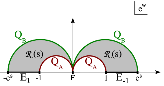
Our analysis in the previous sections shows that in gauges which satisfy the conditions (1.16) the Feynman amplitudes of string field theory reproduce correctly the on-shell amplitudes of open string theory. Unfortunately this argument does not hold for projector gauges since the insertion of $e^{-\Lambda_{(g)}{\cal L}_{(g)}}$ into an amplitude does not in general localize the contribution to the boundary of the moduli space in the limit as $\Lambda_{(g)}\to\infty$ . To demonstrate this, we shall choose the familiar Schnabl gauge but a similar analysis can be done for any projector gauge of the type discussed below (2.76).

As described in Fig. 13(b) the region ${\cal R}(s)$ for Schnabl gauge looks singular in the $w$ frame since the real parts of the midpoints ( $\theta=\pi/2$ ) of the boundary components $Q_{A}$ and $Q_{B}$ reach $-\infty$ . A better understanding of the situation is obtained by examining this region in the $\tilde{z}=e^{w}$ plane. This has been shown in Fig. 16(a).¹⁸¹⁸ 18 For comparison, we also show the strip ${\cal R}(s)$ in Fig. 16(b) in the frame obtained from $\tilde{z}$ by the BPZ map $\tilde{z}\to-1/\tilde{z}$ . The surface ${\cal R}(s)$ appears as two semi-infinite vertical strips. Up to a constant rescaling, this frame is the familiar sliver frame. As can be seen from this figure, the midpoints on the boundaries $Q_{A}$ and $Q_{B}$ fuse at a single point $F$ , dividing the region ${\cal R}(s)$ into two components. This can also be understood as follows. The $\tilde{z}$ coordinate is of the general form (4.44), and thus $-{\cal L}_{(g)}$ can be interpreted as the generator of rescalings $L_{0}$ in the $\tilde{z}$ frame. As the fusion point $F$ is the origin of the $\tilde{z}$ -frame, the action of ${\cal L}_{(g)}$ leaves $F$ invariant and therefore $e^{-s{\cal L}_{(g)}}$ fails to separate completely the boundary components $Q_{A}$ and $Q_{B}$ of ${\cal R}(s)$ . In the computation of $\langle\Sigma_{A}|e^{-s{\cal L}_{(g)}}|\Sigma_{B}\rangle$ , the boundaries $Q_{A}$ and $Q_{B}$ are glued to the coordinate curves $P_{A}$ and $P_{B}$ of the Riemann surfaces $\Sigma_{A}$ and $\Sigma_{B}$ . The result is a correlation function on the surface $\Sigma_{AB}(s)$ in which the midpoints of the coordinate curves of $\Sigma_{A}$ and $\Sigma_{B}$ remain fused for all values of $s$ . Therefore the surface $\Sigma_{AB}(s)$ does not in general exhibit open string degeneration in the limit $s\to\infty$ .

The simplest example of this phenomenon occurs in the computation of the four-point function in the Schnabl gauge: the matrix element of $e^{-\Lambda L}e^{-\Lambda^{\star}L^{\star}}$ between two three-string vertices corresponds to the contribution from a finite point in the moduli space even for arbitrarily large $\Lambda$ , $\Lambda^{\star}$ as long as $\Lambda$ and $\Lambda^{\star}$ are of the same order [31]. Since $e^{-\Lambda L}$ is the boundary term that arises in the definition of $1/L$ , this shows that $1/L$ is not well defined acting from the left on states of the form $\lim_{\Lambda^{\star}\to\infty}e^{-\Lambda^{\star}L^{\star}}|A*B\rangle$ for a pair of Fock space states $|A\rangle$ , $|B\rangle$ . Similarly $1/L^{\star}$ , acting from the right, is not well defined on the BPZ conjugate of the above state. In the case of the four-point function the problem can be resolved by suitable regularization of the upper limits of integration, treating $L$ and $L^{\star}$ symmetrically [31]. It remains to be seen whether the same regularization of the propagator produces consistent higher point and/or loop amplitudes as well.

6 Discussion

In this paper we studied open string field theory in the class of gauges in which a linear combination ${\cal B}_{(g)}$ of the antighost oscillators annihilates the string field of ghost number $g$ . We derived the Feynman rules and showed that for a wide class of linear $b$ -gauges the string field theory amplitudes reproduce correctly the on-shell S-matrix elements at the tree and the loop levels. Our analysis, however, does not work for all linear $b$ -gauges, – certain regularity conditions must be satisfied in order for it to work. In particular Schnabl gauge, which has provided a geometric and algebraic framework to explicitly construct classical solutions in open string field theory, fails to satisfy these regularity conditions.

Schnabl gauge has been known to be subtle for string perturbation theory for some time. In particular the analysis of [31] shows that a consistent off-shell Veneziano amplitude can be obtained only through a delicate regularization scheme. Higher $n$ -point tree amplitudes and loop amplitudes have not been studied, so there could be additional difficulties there. Our analysis shows that these difficulties can be traced back to the difficulty in defining the inverse of ${\cal L}_{(g)}\equiv\{Q,{\cal B}_{(g)}\}$ that enters the definition of the propagator. The usual representation of $1/{\cal L}_{(g)}$ in terms of an integral over a Schwinger parameter fails due to a non-vanishing boundary term from the upper limit of integration. This in turn can be traced back to the fact that the conformal transformation generated by ${\cal L}_{(g)}$ in this gauge does not move the open string midpoint. As a result, in the representation as an integral over the Schwinger parameter, the insertion of $1/{\cal L}_{(g)}$ does not effectively separate the surfaces it connects even in the limit where the Schwinger parameter becomes large. Notwithstanding these complications it is still possible that suitable regularization of the propagator involving cut-offs on the Schwinger parameters and a prescription to take limits will render the higher point functions at tree and/or loop level consistent. This deserves further study.

We constructed a one-parameter family of regular gauges which interpolates between Siegel and Schnabl gauge. It would be interesting to see if this parameter can be used to regularize Schnabl gauge. If this is possible, off-shell amplitudes in Schnabl gauge could be defined by taking the limit, as we approach Schnabl gauge, of the amplitudes computed within this family. These results can then be compared to the off-shell Veneziano amplitudes computed in [31, 30] with a different regularization prescription.

Another surprising feature of the Schnabl gauge found in [31] is that the off-shell Veneziano amplitude does not exhibit off-shell factorization. We have explained this geometrically and learned that only in Siegel gauge we expect off-shell factorization. In other regular $b$ -gauges off-shell factorization is expected to fail because as we attach a propagator to the coordinate curve associated with a puncture the natural local coordinate induced by the strip domain ${\cal R}(s)$ fails to agree with the original local coordinate.¹⁹¹⁹ 19 We thank Leonardo Rastelli for raising the question of off-shell factorization. This is, however, not a failure of the gauge choice. Despite being a desirable feature, off-shell factorization is not a requirement we need to impose on a choice of gauge. The lack of off-shell factorization both for $B^{\lambda}$ gauges and for Schnabl gauge is consistent with our proposal to define amplitudes in Schnabl gauge by taking the $\lambda\to 0$ limit.

Even if open string perturbation theory fails in Schnabl gauge, it does not by itself signal any problem for the classical solutions constructed in this gauge since they satisfy the complete set of open string field theory equations of motion. Nevertheless, it would be interesting to obtain exact analytic solutions in gauges where perturbation theory is well defined, like Siegel gauge. This will facilitate understanding open string perturbation theory around the tachyon vacuum – in particular open string loop diagrams which are expected to contain information about closed string theory. It will be interesting to see if by making an appropriate gauge transformation we can convert Schnabl gauge solutions into solutions in the family of regular gauges interpolating between the Schnabl gauge and the Siegel gauge. This analysis may be facilitated by the existence of a continuous family of gauges: we can now look for infinitesimal gauge transformations which convert a solution in one gauge to another in a nearby gauge.

Regular linear $b$ -gauges satisfy the consistency conditions required for a well defined perturbation theory and our analysis provides an explicit geometric description of the $1/{\cal L}_{(g)}$ operator. Representing it as an integral of $e^{-s{\cal L}_{(g)}}$ over the Schwinger parameter $s$ we find that insertion of $e^{-s{\cal L}_{(g)}}$ into a correlation function inserts a strip into the Riemann surface on which the correlator is being computed. Unlike the case in Siegel gauge, for which the corresponding operator $1/L_{0}$ inserts rectangular strips, here the ends of the strips which connect to the rest of the Riemann surface are ragged. For regular linear $b$ -gauges, the ends of the strip are parameterized by a continuous curve $\gamma$ that satisfies the following properties: (i) it is smooth, (ii) it has finite width, (iii) it has finite horizontal spread, (iv) it is reflection symmetric about the horizontal line that bisects the strip, (v) it is perpendicular to the open string boundaries, and, (vi) it does not intersect any horizontal line more than once. These properties followed from our conditions on the vector field associated with the gauge choice.

It would be interesting to see if consistent linear $b$ -gauges arise with weaker conditions. In particular, any vector field that results in a curve $\gamma$ that satisfies the above properties (ii)–(vi) but is only continuous as opposed to smooth, may be acceptable. This is plausible because the strip domain is still well-defined and reaches open string degeneration for large $s$ . This class of gauges includes all regular linear $b$ -gauges, but also includes gauges in which the vector field associated with ${\cal B}_{(g)}$ is not analytic in a neighborhood of the unit circle and may even have zeros on the unit circle. Gauges associated with the so-called “wedge states” are of this type. The corresponding curves $\gamma$ are continuous but not smooth.

An important difference between a general linear $b$ -gauge and the Siegel gauge is that the propagator in the former gauge contains two $1/{\cal L}_{(g)}$ operators (of different ghost numbers) separated by an insertion of a BRST charge. Thus in the Riemann surface picture, a propagator will be represented by a pair of strips separated by the line integral of the BRST current. This general structure of the propagator, with two Schwinger parameters and a BRST insertion in between, suggests that a new definition of open string amplitudes may be possible. The usual Polyakov definition of open string amplitudes is closely related to computations in Siegel gauge, where each Schwinger parameter is a true modulus of the Riemann surface. In linear $b$ -gauges there are two Schwinger parameters and one BRST insertion for each modulus. It would be interesting to define, without using string field theory, string amplitudes of the structure suggested by perturbation theory in linear $b$ -gauges.

Acknowledgments: We would like to thank Ian Ellwood, Theodore Erler, Yuji Okawa, Leonardo Rastelli, and Martin Schnabl for discussions and valuable comments on a draft version of this paper. The work of M.K. and B.Z. is supported in part by the U.S. DOE grant DE-FC02-94ER40818. The work of A.S. is supported in part by the JC Bose Fellowship of DST, India and the Morningstar Visiting Professorship at MIT. The work began during the visit of A.S. at the Center for Theoretical Physics at MIT. A.S. would like to acknowledge warm hospitality of the members of CTP during the visit.

References

[1] E. Witten, “Noncommutative Geometry And String Field Theory,” Nucl. Phys. B 268, 253 (1986).
[2] S. B. Giddings, “The Veneziano Amplitude From Interacting String Field Theory,” Nucl. Phys. B 278, 242 (1986).
[3] S. B. Giddings, E. J. Martinec and E. Witten, “Modular Invariance in String Field Theory,” Phys. Lett. B 176, 362 (1986);
B. Zwiebach, “A Proof that Witten’s open string theory gives a single cover of moduli space,” Commun. Math. Phys. 142, 193 (1991);
A. Sen, “Open String Field Theory In Arbitrary Background Field. 2. Feynman Rules And Four Point Amplitudes,” Nucl. Phys. B 334, 395 (1990); “Open string Field Theory In Arbitrary Background Field. 3. n point amplitude,” Nucl. Phys. B 335, 435 (1990).
[4] M. Bochicchio, “Gauge fixing for the field theory of the bosonic string,” Phys. Lett. B 193, 31 (1987);
C. B. Thorn, “Perturbation Theory For Quantized String Fields,” Nucl. Phys. B 287, 61 (1987).
[5] C. B. Thorn, “String Field Theory,” Phys. Rept. 175, 1 (1989).
[6] W. Siegel, “Covariantly Second Quantized String,” Phys. Lett. B 142, 276 (1984); “Covariantly Second Quantized String. 2,” Phys. Lett. B 149, 157 (1984) [Phys. Lett. B 151, 391 (1985)]; “Covariantly Second Quantized String. 3,” Phys. Lett. B 149, 162 (1984) [Phys. Lett. 151B, 396 (1985)].
[7] M. Schnabl, “Analytic solution for tachyon condensation in open string field theory,” Adv. Theor. Math. Phys. 10, 433 (2006) [arXiv:hep-th/0511286].
[8] Y. Okawa, “Comments on Schnabl’s analytic solution for tachyon condensation in Witten’s open string field theory,” JHEP 0604, 055 (2006) [arXiv:hep-th/0603159].
[9] E. Fuchs and M. Kroyter, “On the validity of the solution of string field theory,” JHEP 0605, 006 (2006) [arXiv:hep-th/0603195].
[10] E. Fuchs and M. Kroyter, “Schnabl’s L(0) operator in the continuous basis,” JHEP 0610, 067 (2006) [arXiv:hep-th/0605254].
[11] L. Rastelli and B. Zwiebach, “Solving open string field theory with special projectors,” arXiv:hep-th/0606131.
[12] I. Ellwood and M. Schnabl, “Proof of vanishing cohomology at the tachyon vacuum,” JHEP 0702, 096 (2007) [arXiv:hep-th/0606142].
[13] E. Fuchs and M. Kroyter, “Universal regularization for string field theory,” JHEP 0702, 038 (2007) [arXiv:hep-th/0610298].
[14] Y. Okawa, L. Rastelli and B. Zwiebach, “Analytic solutions for tachyon condensation with general projectors,” arXiv:hep-th/0611110.
[15] T. Erler, “Split string formalism and the closed string vacuum,” JHEP 0705, 083 (2007) [arXiv:hep-th/0611200].
[16] T. Erler, “Split string formalism and the closed string vacuum. II,” JHEP 0705, 084 (2007) [arXiv:hep-th/0612050].
[17] M. Schnabl, “Comments on marginal deformations in open string field theory,” arXiv:hep-th/0701248.
[18] M. Kiermaier, Y. Okawa, L. Rastelli and B. Zwiebach, “Analytic solutions for marginal deformations in open string field theory,” arXiv:hep-th/0701249.
[19] T. Erler, “Marginal Solutions for the Superstring,” JHEP 0707, 050 (2007) [arXiv:0704.0930 [hep-th]].
[20] Y. Okawa, “Analytic solutions for marginal deformations in open superstring field theory,” JHEP 0709, 084 (2007) [arXiv:0704.0936 [hep-th]].
[21] E. Fuchs, M. Kroyter and R. Potting, “Marginal deformations in string field theory,” JHEP 0709, 101 (2007) [arXiv:0704.2222 [hep-th]].
[22] Y. Okawa, “Real analytic solutions for marginal deformations in open superstring field theory,” JHEP 0709, 082 (2007) [arXiv:0704.3612 [hep-th]].
[23] I. Ellwood, “Rolling to the tachyon vacuum in string field theory,” arXiv:0705.0013 [hep-th].
[24] E. Fuchs and M. Kroyter, “Marginal deformation for the photon in superstring field theory,” arXiv:0706.0717 [hep-th].
[25] M. Kiermaier and Y. Okawa, “Exact marginality in open string field theory: a general framework,” arXiv:0707.4472 [hep-th].
[26] T. Erler, “Tachyon Vacuum in Cubic Superstring Field Theory,” arXiv:0707.4591 [hep-th].
[27] M. Kiermaier and Y. Okawa, “General marginal deformations in open superstring field theory,” arXiv:0708.3394 [hep-th].
[28] O. K. Kwon, B. H. Lee, C. Park and S. J. Sin, “Fluctuations around the Tachyon Vacuum in Open String Field Theory,” arXiv:0709.2888 [hep-th].
[29] B. H. Lee, C. Park and D. D. Tolla, “Marginal Deformations as Lower Dimensional D-brane Solutions in Open String Field theory,” arXiv:0710.1342 [hep-th].
[30] H. Fuji, S. Nakayama and H. Suzuki, “Open string amplitudes in various gauges,” JHEP 0701, 011 (2007) [arXiv:hep-th/0609047].
[31] L. Rastelli and B. Zwiebach, “The off-shell Veneziano amplitude in Schnabl gauge,” arXiv:0708.2591 [hep-th].
[32] M. Asano and M. Kato, “New covariant gauges in string field theory,” arXiv:hep-th/0611189.
[33] C. R. Preitschopf, C. B. Thorn and S. A. Yost, “Superstring field theory,” Nucl. Phys. B 337, 363 (1990).
[34] M. R. Gaberdiel and B. Zwiebach, “Tensor constructions of open string theories I: Foundations,” Nucl. Phys. B 505, 569 (1997) [arXiv:hep-th/9705038].

1 Introduction and summary

2 General linear bb-gauges

2.1 Gauge conditions, ghosts, and gauge fixed action

2.2 The propagator

2.3 Properties of the propagator

2.4 Constraints on linear bb-gauges

2.5 Examples

3 Analysis of on-shell amplitudes

3.1 Decoupling of pure gauge states

3.2 Proof of equivalence to Siegel gauge amplitudes

4 Conditions from consistent Schwinger representations of 1/ℒ(g)1/{\cal L}_{(g)}

4.1 Gluing surface states with e−s​ℒ(g)e^{-s{\cal L}_{(g)}} insertions

4.1.1 The strip domain ℛ⁡(s){\cal R}(s)

4.1.2 Properties of the sewing curve γ\gamma

4.1.3 Coordinate frames and examples

4.2 Degeneration and the s→∞s\to\infty limit

4.3 Schwinger parametrization of the propagator

5 On-shell amplitudes revisited

5.1 Decoupling of trivial states

5.2 Correct on-shell amplitudes

5.3 Projector gauges

6 Discussion

References

2 General linear $b$ -gauges

2.4 Constraints on linear $b$ -gauges

4 Conditions from consistent Schwinger representations of $1/{\cal L}_{(g)}$

4.1 Gluing surface states with $e^{-s{\cal L}_{(g)}}$ insertions

4.1.1 The strip domain ${\cal R}(s)$

4.1.2 Properties of the sewing curve $\gamma$

4.2 Degeneration and the $s\to\infty$ limit