A limiting velocity for quarkonium propagation in a strongly coupled
plasma via AdS/CFTPreprint: MIT-CTP-3912
CERN-PH-TH/2007-232
CAS-KITPC/ITP-024
Abstract:
We study the dispersion relations of mesons in a particular hot strongly coupled supersymmetric gauge theory plasma. We find that at large momentum the dispersion relations become , where the limiting velocity is the same for mesons with any quantum numbers and depends only on the ratio of the temperature to the quark mass . We compute and in terms of the meson quantum numbers and . The limiting meson velocity becomes much smaller than the speed of light at temperatures below but close to , the temperature above which no meson bound states at rest in the plasma are found. From our result for , we find that the temperature above which no meson bound states with velocity exist is , up to few percent corrections. We thus confirm by direct calculation of meson dispersion relations a result inferred indirectly in previous work via analysis of the screening length between a static quark and antiquark in a moving plasma. Although we do not do our calculations in QCD, we argue that the qualitative features of the dispersion relation we compute, including in particular the relation between dissociation temperature and meson velocity, may apply to bottomonium and charmonium mesons propagating in the strongly coupled plasma of QCD. We discuss how our results can contribute to understanding quarkonium physics in heavy ion collisions.
Keywords:
AdS/CFT correspondence, Thermal Field Theory1 Introduction
The radii of the tightly bound heavy quark-antiquark systems of the charmonium (, , , …) and bottomonium (, , …) families provide a unique set of decreasing length scales in strong interaction physics. On general grounds, it is expected that the attraction between a heavy quark and an anti-quark is sensitive to the medium in which the bound state is embedded, and that this attraction weakens with increasing temperature. In the context of ultra-relativistic nucleus-nucleus collisions, the radii of some quarkonia states correspond to fractions of the natural length scale displayed by the medium produced in heavy ion collisions, namely fractions of its inverse temperature . Such scale considerations support the idea that measurements of the medium-modification or dissociation of quarkonia can characterize properties of the QCD matter produced in heavy ion collisions.
Matsui and Satz were the first to highlight the role of quarkonium in the study of hot QCD matter [1]. They suggested that -suppression is a signature for the formation of deconfined quark-gluon plasma (QGP). More precisely, they argued that in comparison to proton-proton or proton-nucleus collisions, the production of mesons should be suppressed if quark-gluon plasma is formed in sufficiently energetic nucleus-nucleus collisions, since the screened interaction of a and a in QGP would not bind them [1]. The theoretical basis for this argument has been clarified considerably within the last two decades [2]. Model-independent calculations of the static potential between a heavy quark and anti-quark have been performed in lattice-regularized QCD, valid at strong coupling [3, 4, 5, 6, 7, 8]. In lattice calculations without dynamical quarks, at temperature and large separation this potential rises linearly with , consistent with confinement. At nonzero temperature, the potential weakens and levels off at large distances; with increasing temperature, the distance at which this screening occurs decreases. This behavior of the static potential has been mapped out for hot QCD matter both without [4] and with [5, 6] dynamical quarks. However, the physical interpretation of static potentials at finite temperature rests on additional assumptions. For instance, even if a potential supports a bound state with several MeV binding energy, it remains unclear which physics can be attributed to such a state in a heat bath of MeV temperature. Such issues do not arise in a discussion of quarkonium mesons based directly on their Minkowski space spectral functions or dispersion relations. In recent years, the spectral functions have been characterized by lattice calculations of the Euclidean correlation functions to which they are analytically related, again in hot QCD matter both without [9] and with [10] dynamical quarks. The use of these calculations of finitely many points on a Euclidean correlator to constrain the Minkowski space spectral function of interest via the Maximum Entropy Method requires further inputs — for example smoothness assumptions or information on the analytic properties of the spectral function [9, 10]. At high enough temperatures that quark-gluon plasma becomes weakly coupled, a complementary analytical approach based upon resummed hard-thermal-loop perturbation theory becomes available [11]. These calculations have the advantage that analytical continuation from Euclidean to Minkowski space does not introduce additional uncertainties, but it remains unclear to what extent they can treat a strongly coupled quark-gluon plasma. In broad terms, all these calculations support the qualitative picture behind the original suggestion of Matsui and Satz that color screening in the quark-gluon plasma is an efficient mechanism for quarkonium dissociation. In addition, these studies support the picture of a sequential dissociation pattern [12], in which loosely bound, large, quarkonia such as the and cease to exist close to , the temperature of the crossover between hadronic matter and quark-gluon plasma, whereas more tightly bound, smaller, states dissociate only at significantly higher temperatures. In particular, mesons continue to exist for a range of temperatures above the QCD phase transition and dissociate only above a temperature that lies between and [12]. The observation of bound-state-specific quarkonia suppression patterns could thus provide detailed information about the temperature attained in heavy ion collisions.
On the experimental side, there are by now data from the NA50 and NA60 experiments at the CERN SPS and from the PHENIX experiment at RHIC demonstrating that the production of mesons is suppressed in ultra-relativistic nucleus-nucleus collisions compared to proton-proton or proton-nucleus collisions at the same center of mass energy [13]. However, due to lack of statistics and resolution, an experimental characterization of other charmonium states (, , …) has not yet been possible at RHIC, and bottomonium states have not yet been characterized in any nucleus-nucleus collisions. Moreover, the observed yield of mesons is expected to receive significant decay contributions from and , meaning that the observed suppression of mesons may originate only in the suppression of the larger and states [12], or may indicate a suppression in the number of primary mesons themselves in addition. Thus, at present an experimental test of the sequential quarkonium suppression pattern is not in hand. It is expected that the LHC heavy ion program will furnish such a test, since two LHC experiments [14] have demonstrated capabilities for discriminating between the different states of the charmonium and bottomonium families.
From the existing data in ultra-relativistic heavy ion collisions and their phenomenological interpretation, it has become clear that an unambiguous characterization of color screening effects in the quarkonium systems requires good experimental and theoretical control of several confounding factors. These include in particular control over the spatio-temporal evolution of the medium, control over the time scale and mechanism of quarkonium formation, as well as control over the effects of quarkonium propagation through the medium. We now comment on these three sources of uncertainty in more detail:
First, there is ample evidence by now that the systems produced in ultra-relativistic heavy ion collisions display effects of position-momentum correlated motion (a.k.a. flow), which are as important as the effects of random thermal motion [15]. Moreover, the energy density achieved in these collisions drops rapidly with time as the matter expands and falls apart after approximately 10 fm/c. As a consequence, the modeling of quarkonium formation in heavy ion collisions cannot be limited to a description of heavy quark bound states in a heat bath at constant temperature (which is the information accessible in ab initio calculations in lattice-regularized QCD). The effects of a rapid dynamical evolution during which the relevant degrees of freedom in the medium change from partonic to hadronic must be taken into account.
Second, regarding the formation process, the conversion of a heavy quark pair produced in a hard collision into a bound quarkonium state is not fully understood, even in the absence of a medium. There are different production models, which all have known limitations and for which a systematic calculation scheme remains to be fully established (for a short review of these issues, see [16]). The need for further clarification of the vacuum case has even led to suggestions that nuclear matter could serve as a filter to distinguish between different production mechanisms [17, 18]. However, it has also been pointed out that there may be a novel quarkonium production mechanism operating only in ultra-relativistic heavy ion collisions at RHIC and at the LHC [19]: charm quarks may be so abundant in these collisions that and quarks produced separately in different primary hard scattering interactions may find each other and combine, contributing significantly to charmonium production at soft and intermediate transverse momentum. To a lesser extent, this mechanism may also contribute to the production of Upsilon mesons. Identifying and characterizing such a novel formation process is of considerable interest, since recombination is likely to be quadratically sensitive to the phase space density of charm and thus to properties of the produced matter. On the other hand, if realized in nature recombination also implies that quarkonium spectra at soft and intermediate transverse momenta are determined predominantly during the late hadronization stage and cannot be viewed as probes which test color screening in the quark gluon plasma. This would indicate that the high transverse momentum regime (say above 5-8 GeV) of quarkonium spectra, which should not be significantly affected by recombination, is better suited for tests of the fundamental color screening effects predicted by QCD. However, the sensitivity of high transverse momentum spectra to properties of the medium remains to be established. In particular, quarkonium formation or dissociation proceeds on a time scale comparable to the size of the bound state in its rest frame, meaning that quark-antiquark pairs with very high transverse velocity may escape the finite-sized droplet of hot matter produced in a heavy ion collision before they have time to form a meson, meaning in turn that screening effects cease to play a role in quarkonium production above some very high transverse momentum [20]. At lower transverse momenta, where screening does play a role, one must nevertheless understand for how long quarkonium is exposed to the medium and how readily it dissociates if moving relative to that medium. For quarkonium at high transverse momentum, the time of exposure to the medium depends on the geometry of the collision region, which determines the in-medium path length, and it depends on the propagation velocity. The results contained in this paper give novel input to modeling this process by demonstrating that the real part of the finite temperature quarkonium dispersion relation can differ significantly from the vacuum one, and can imply a limiting quarkonium propagation velocity which is much smaller than , the velocity of light in vacuum. Our results indicate that at temperatures close to but below that at which a given quarkonium state dissociates, these mesons move through a strongly coupled quark-gluon plasma at a velocity that is much smaller than even if they have arbitrarily high transverse momentum. Certainly this means that the formation time arguments of [20] will need rethinking before they can be applied quantitatively.
Third, we turn to the question of how the relative motion of quarkonium with respect to the local rest frame of the medium affects quarkonium production. As discussed above, the standard vacuum relation between the momentum of a quarkonium state and its velocity can be altered in the presence of a medium and this effect may be phenomenologically relevant. In addition, it is expected that a finite relative velocity between the medium and the bound state enhances the probability of dissociation [21]. In a recent strong coupling calculation of hot supersymmetric QCD, three of us have have shown [22, 23] that the sceening length for a heavy quark-antiquark pair decreases with increasing velocity as , with the Lorentz boost factor. This suggests that a quarkonium state that is bound at at a given temperature could dissociate above some transverse momentum due to the increased screening, providing a significant additional source of quarkonium suppression at finite transverse momentum. The present work started from the motivation to establish how this velocity scaling manifests itself in a description of mesons at finite temperature, rather than via drawing inferences from a calculation of the screening length that characterizes the quark-antiquark potential. This motivation is analogous to that behind going from lattice QCD calculations of the static potential in QCD to calculations of the Minkowski space meson spectral function. We shall do our calculation in a different strongly coupled gauge theory plasma, in which we are able to do this investigation for mesons with nonzero velocity. We shall see that the critical velocity for the dissociation of quarkonium inferred from the velocity scaling of the screening length also appears as a limiting velocity for high-momentum quarkonium propagation in the hot non-abelian plasma.
Finally, the characterization of color screening also depends on the experimental and theoretical ability to separate its effects on quarkonium production from effects arising during the late time hadronic phase of the heavy ion collision. In particular, it has been noted early on that significant charmonium suppression may also occur in confined hadronic matter [24]. However, it has been argued on the basis of model estimates for the hadronic dissociation cross section [25] that dissociation in a hadronic heat bath is much less efficient than in a partonic one. The operational procedure for separating such hadronic phase effects is to measure them separately in proton-nucleus collisions [26], and to establish then to what extent the number of mesons produced in nucleus-nucleus collisions drops below the yield extrapolated from proton-nucleus collisions [13, 27].
The above discussion highlights the extent to which an understanding of quarkonium production in heavy ion collisions relies on theoretical modelling as the bridge between experimental observations and the underlying properties of hot QCD matter. This task involves multiple steps. It is of obvious interest to validate or constrain by first principle calculations as many steps as possible, even in a simplified theoretical setting. The present work is one of a number of recent developments [28] that explore to what extent techniques from string theory, in particular the AdS/CFT correspondence, can contribute to understanding processes in hot QCD by specifying how these processes manifest themselves in a large class of hot strongly coupled non-abelian gauge theories. Although it is not known how to extend the AdS/CFT correspondence to QCD, there are several motivations for turning to this technique. First, there are a growing number of explicit examples which indicate that a large class of thermal non-abelian field theories with gravity duals share commonalities such that their properties in the thermal sector are either universal at strong coupling, i.e. independent of the microscopic dynamics encoded in the particular quantum field theory under study, or their properties are related to each other by simple scaling laws e.g. depending on the number of elementary degrees of freedom. This supports the working hypothesis that by learning something about a large class of strongly coupled thermal non-abelian quantum field theories, one can gain guidance towards understanding the thermal sector of QCD. Second, the AdS/CFT correspondence allows for a technically rather simple formulation of problems involving real-time dynamics. This is very difficult in finite temperature lattice-regularized calculations, which exploit the imaginary time formalism. In particular, this is the reason why so far lattice QCD calculations treat only static quark-antiquark pairs in the plasma, and why the only nonperturbative calculation of the velocity dependence of quarkonium dissociation exploits the AdS/CFT correspondence. Third, data from experiments at RHIC pertaining to many aspects of the matter produced in heavy ion collisions indicate that this matter is strongly coupled. Since the AdS/CFT correspondence provides a mapping of difficult nonperturbative calculations in a quantum field theory with strong coupling onto relatively simple, semi-classical calculations in a gravity dual, it constitutes a novel — and often the only — technique for addressing dynamical questions about hot strongly coupled non-abelian matter, questions that are being raised directly by experimental results on QCD matter coming from RHIC.
We have focussed in this Section on the larger context for our results. In Section 2, which is an introduction in a more narrow sense, we review the past results which serve as an immediate motivation for our work, in particular the screening length that characterizes the potential between a static quark and antiquark in a moving plasma wind. Adding fundamental quarks with finite mass , and hence mesons, into SYM theory requires adding a D7-brane in the dual gravity theory, as we review in Section 3. The fluctuations of the D7-brane are the mesons, as we review for the case of zero temperature in Section 3. In Section 4 we set up the analysis of the mesons at nonzero temperature, casting the action for the D7-brane fluctuations in a particularly geometric form, written entirely in terms of curvature invariants. Parts of the derivation are explained in more detail in Appendix A. With all the groundwork in place, in Section 5 we derive the meson dispersion relations. In addition to obtaining them numerically without taking any limits as has been done previously [29], we are able to calculate them analytically in three limits: first, upon taking the low temperature limit at fixed ; second, upon taking the low temperature limit at fixed ; and third, using insights from the first two calculations, at large for any temperature. At large we find
| (1.1) |
where is independent of meson quantum numbers, depending only on . turns out to be given by the local speed of light at the “tip of the D7-brane”, namely the place in the higher dimensional gravity dual theory where the D7-brane comes closest to the black hole [29]. We compute and in terms of meson quantum numbers and . Our result for the limiting velocity for mesons at a given temperature can be inverted, obtaining , the temperature above which no mesons with velocity are found. We find that up to few percent corrections, our result can be summarized by
| (1.2) |
where is the temperature at which zero-velocity mesons dissociate, obtained in previous work and introduced in Section 3. As we discuss in Section 2, our results obtained by direct calculation of meson dispersion relations confirm inferences reached (in two different ways) from the analysis of the screened potential between a static quark and antiquark in a hot plasma wind. In Section 6, we close with a discussion of potential implications of these dispersion relations for quarkonia in QCD as well as a look at open questions. The dispersion relations that we calculate in this paper describe how mesons propagate and so affect a class of observables, but determining whether quarkonium meson formation from a precursor quark-antiquark pair is suppressed by screening is a more dynamical question that can at present be addressed only by combining our calculation and the more heuristic results of [23].
2 From screening in a hot wind to moving mesons
In the present work, we shall use the AdS/CFT correspondence to study the propagation of mesonic excitations moving through a strongly coupled hot quark-gluon plasma. In this Section, however, we introduce what we have learned from the simpler calculation of the potential between a test quark-antiquark pair moving through such a medium. This will allow us to pose the questions that we shall address in the present paper.
The simplest example of the AdS/CFT correspondence is provided by the duality between super Yang-Mills (SYM) theory and classical gravity in [30]. super Yang-Mills (SYM) theory is a conformally invariant theory with two parameters: the rank of the gauge group and the ’t Hooft coupling . In the large and large limit, gauge theory problems can be solved using classical gravity in geometry. We shall work in this limit throughout this paper.
In SYM theory at zero temperature, the static potential between a heavy external quark and antiquark separated by a distance is given in the large and large limit by [31, 32]
| (2.1) |
where the behavior is required by conformal invariance. This potential is obtained by computing the action of an extremal string world sheet, bounded at ( being the fifth dimension of ) by the world lines of the quark and antiquark and “hanging down” from these world lines toward smaller . At nonzero temperature, the potential becomes [33]
| (2.2) |
In (2), at there is a change of dominance between different saddle points and the slope of the potential changes discontinuously. When , the potential is determined as at zero temperature by the area of a string world sheet bounded by the worldlines of the quark and antiquark, but now the world sheet hangs down into a different five-dimensional spacetime: introducing nonzero temperature in the gauge theory is dual to introducing a black hole horizon in the five-dimensional spacetime. When , reduces to its zero temperature behavior (2.1). When , has the behavior [34]
| (2.3) |
with , and constants all of which are proportional to . This large- potential arises from two disjoint strings, each separately extending downward from the quark or antiquark all the way to the black hole horizon, exchanging supergravity modes the lightest of which has a mass given by . (There are somewhat lighter modes with nonzero R-charge, but these are not relevant here [35].) It is physically intuitive to interpret as the screening length of the plasma since at the qualitative behavior of the potential changes. Similar criteria are used in the definition of screening length in QCD [8], although in QCD there is no sharply defined length scale at which screening sets in. Lattice calculations of the static potential between a heavy quark and antiquark in QCD indicate a screening length in hot QCD with two flavors of light quarks [6] and in hot QCD with no dynamical quarks [4]. The fact that there is a sharply defined in (2) is an artifact of the limit in which we are working.11 1 The theoretical advantage of using to define a screening length as advocated in [34] is that it can be precisely defined in SYM theory at finite and , as well as in QCD, as it characterizes the behavior of the static potential in the limit. The disadvantage of this proposal from a phenomenological point of view is that quarkonia are not sensitive to the potential at distances much larger than their size. For questions relevant to the stability of bound states, therefore, the length scale determined by the static potential that is phenomenologically most important is that at which the potential flattens. Although this length is not defined sharply in QCD, it is apparent in lattice calculations and can be defined operationally for practical purposes [4, 6]. This seems most analogous to in (2), and we shall therefore continue to refer to as the screening length, as in the original literature [33]. Note that is larger than by a purely numerical factor .
In [22, 23], three of us studied the velocity scaling of the screening length in super-Yang-Mills theory and found that22 2 In [22, 23] was defined using a slightly different quantity than in (2), such that for a quark-antiquark at rest. For technical reasons, this other definition was more easily generalizable to nonzero velocity.
| (2.4) |
where is the angle between the orientation of the quark-antiquark dipole and the velocity of the moving thermal medium in the rest frame of the dipole. is only weakly dependent on both of its arguments. That is, it is close to constant. So, to a good approximation we can write
| (2.5) |
This result, also obtained in [36] and further explored in [37, 38, 39], has proved robust in the sense that it applies in various strongly coupled plasmas other than SYM [37, 38, 39]. The velocity dependence of the screening length (2.5) suggests that in a theory containing dynamical heavy quarks and meson bound states (which SYM does not) the dissociation temperature , defined as the temperature above which mesons with a given velocity do not exist, should scale with velocity as [22]
| (2.6) |
since should be the temperature at which the screening length is comparable to the size of the meson bound state. The scaling (2.6) then indicates that slower mesons can exist up to higher temperatures than faster ones. In this paper, we shall replace the inference that takes us from the calculated result (2.5) to the conclusion (2.6) by a calculation of the properties of mesons themselves, specifically their dispersion relations. We shall reproduce (2.6) in this more nuanced setting, finding few percent corrections to the basic scaling result inferred previously.
The results (2.5) and (2.6) have a simple physical interpretation which suggests that they could be applicable to a wide class of theories regardless of specific details. First, note that since , both (2.5) and (2.6) can be interpreted as if in their rest frame the quark-antiquark dipole experiences a higher effective temperature . Although this is not literally the case in a weakly coupled theory, in which the dipole will see a redshifted momentum distribution of quasiparticles coming at it from some directions and a blueshifted distribution from others [21], we give an argument below for how this interpretation can nevertheless be sensible. The result (2.5) can then be seen as validating the relevance of this interpretation in a strongly coupled plasma. The argument is based on the idea that quarkonium propagation and dissociation are mainly sensitive to the local energy density of the medium. Now, in the rest frame of the dipole, the energy density (which we shall denote by ) is blue shifted by a factor and since in a conformal theory, the result (2.5) is as if quarks feel a higher effective temperature given by .33 3 Applying a Lorentz boost to yields . Including the factor makes this argument reproduce the result (2.4), including the weak velocity dependence in the function , more quantitatively than merely tracking the powers of . Lattice calculations indicate that the quark-gluon plasma in QCD is nearly conformal over a range of temperatures , with an energy density where is a constant about of the free theory value [40]. So it does not seem far-fetched to imagine that (2.5) could apply to QCD. We should also note that AdS/CFT calculations in other strongly coupled gauge theories with a gravity description are consistent with the interpretation above [38] and that for near conformal theories the deviation from conformal theory behavior appears to be small [38]. If a velocity scaling like (2.5) and (2.6) holds for QCD, it can potentially have important implications for quarkonium suppression in heavy ion collisions, as we have discussed in Section 1 and will return to in Section 6.
While the argument leading from (2.5) to (2.6) is plausible, it is more satisfying to have a set-up within which one can study mesons directly. Direct study of meson bound states will also yield more insights than the study of the screening length from the potential. It is the purpose of this paper to examine this issue in a specific model with dynamical flavors.
Before beginning our analysis, let us first note a curious feature regarding the quark potential observed in [22, 23]. There one introduces a probe brane near the boundary of the AdS5 black hole geometry with open strings ending on it corresponding to fundamental “test quarks” of mass . It was found that for any given quark mass , there exists a maximal velocity given by
| (2.7) |
beyond which there is no potential between the pair for any value of their separation larger than their Compton wavelength, i.e. for any distance at which a potential can be defined. This result can be interpreted as saying that for any given and , it is impossible to obtain bound states beyond (2.7), i.e. as indicating that there is a velocity bound (a “speed limit”) for the mesons. One can also turn (2.7) around and infer that for any large and close to 1, the dissociation temperature is given by
| (2.8) |
which is consistent with (2.6). Note that the above argument is at best heuristic since SYM itself does not contain dynamical quarks and thus genuine mesons do not exist. In the present paper, however, we shall see by deriving them from meson dispersion relations that (2.7) and (2.8) are precisely correct in the limit of large quark mass once we introduce fundamentals, and hence mesons, into the theory. We shall also find that the more dynamical, albeit heuristic, interpretation of (2.7) as a velocity beyond which a quark and antiquark do not feel a potential that can bind them remains of value.
3 D3/D7-brane construction of mesons
In this Section we review the gravity dual description of strongly coupled SYM theory with gauge group coupled to hypermultiplets in the fundamental representation of , introduced in [41] and studied in [42, 43, 44, 45, 46, 47, 48, 49, 50, 29, 51, 52, 53]. We will first describe the theory at zero temperature and then turn to nonzero temperature. We will work in the limit , and finite (in fact ). In the deconfined strongly coupled plasma that this theory describes, heavy quark mesons exist below a dissociation temperature that, for mesons at rest, is given by [43, 49, 50, 29]. In Section 5 we shall calculate the dispersion relations for these mesons, namely the meson spectrum at nonzero momentum and in so doing determine directly, rather than by inference as described in Section 2.
3.1 Zero temperature
Consider a stack of coincident D3-branes and coincident D7-branes in 9+1-dimensional Minkowski space, which we represent by the array
| (3.1) |
which denotes in which of the 9+1 dimensions the D3- and D7-branes are extended, and in which they occupy only points. The D3-branes sit at the origin of the 89-plane, with denoting the distance between the D3- and the D7-branes in the 89-plane. Without loss of generality (due to rotational symmetry in 89-plane), we can take the D7-branes to be at . This is a stable configuration and preserves one quarter of the total number of supersymmetries, meaning that it describes an supersymmetric gauge theory as we now sketch [41].
The open string sector of the system contains 3-3 strings, both of whose ends lie on one of the D3-branes, 7-7 strings ending on D7-branes, and 3-7 and 7-3 strings stretching between D3- and D7-branes. In the low energy limit
| (3.2) |
all the stringy modes decouple except for: (i) the lightest modes of the 3-3 strings, which give rise to an SYM theory in 3+1-dimensional Minkowski space; (ii) the lightest modes of the 3-7 and 7-3 strings, which give rise to hypermultiplets in the gauge theory transforming under the fundamental representation of . The whole theory thus has supersymmetry. We will call hypermultiplets quarks below even though they contain both fermions and bosons. The mass of the quarks is given by
| (3.3) |
where is the tension of the strings.
In the limit
| (3.4) |
the above gauge theory has a gravity description [41] in terms of D7-branes in the near-horizon geometry of the D3-branes, which is with a metric
| (3.5) | |||||
where and is the metric on a 5-sphere. is the curvature radius of AdS and is related to the Yang-Mills theory ’t Hooft coupling by
| (3.6) |
The string coupling constant is related to the gauge theory parameters by
| (3.7) |
where is defined according to standard field theory conventions and is twice as large as the Yang-Mills gauge coupling defined according to standard string theory conventions. In this zero temperature setting, the embedding of the D7-branes in the geometry (3.5) can be read directly from (3.1). The D7-brane worldvolumes fill the coordinates, with , and are located at the point in the 89-plane. Since remains finite in the large limit, the gravitational back-reaction of the D7-branes on the spacetime of the D3-branes (3.5) may be neglected.
The dictionary between the gauge theory and its dual gravity description can thus be summarized as follows. On the gauge theory side we have two sectors: excitations involving adjoint degrees of freedom only and excitations involving the fundamentals. The first type of excitations correspond to closed strings in as in the standard AdS/CFT story. The second type is described by open strings ending on the D7-branes44 4 We will not consider baryons in this paper.. In particular, the low-lying (in a sense that we shall define later) meson spectrum of the gauge theory can be described by fluctuations of and gauge fields on D7-branes. We shall focus on the fluctuations of on the D7-brane (equivalently, the fluctuations of the position of the D7-brane in the plane) which describe scalar mesons. There are also gauge fields localized within the D7-brane, and their fluctuations describe vector mesons. The description of the vector mesons is expected to be similar to that of the scalar mesons. We shall limit our presentation entirely to the scalar mesons. We shall take , meaning that the gauge theory is specified by the parameters , and which are related to their counterparts in the dual gravity theory by (3.6), (3.7) and (3.3). We see that the limit corresponds to , making the string theory weakly coupled. Considering the theory with the parameter taken to corresponds to taking the string tension to infinity. These limits justify the use of the classical gravity approximation in which we consider strings moving in a background spacetime.
For later generalization to finite temperature, it is convenient to describe the D7-brane in a coordinate system which makes the symmetries of its embedding more manifest. We split the factor in the last term of (3.5) into (i.e. parts longitudinal and transverse to the D7-brane) and express them in terms of polar coordinates respectively. More explicitly,
| (3.8) |
The metric (3.5) then becomes
| (3.9) |
The D7-brane now covers and sits at and . Note that in the radial direction the D7-brane extends from , at which the size of the three-sphere becomes zero, to . The point corresponds to .
We now briefly describe how to find the low-lying meson spectrum described by the fluctuations of . The action of the D7-brane is given by the Dirac-Born-Infeld action
| (3.10) |
where the (with ) denote the worldvolume coordinates of the D7 brane and is the induced metric in the worldvolume
| (3.11) |
The value of the D7-brane tension, , will play no role in our considerations. The spacetime metric is given by (3.9) and describe the embedding of the D7-brane, where runs through all spacetime coordinates. The action (3.10) is invariant under the coordinate transformations . We can use this freedom to set , and the embedding described below equation (3.9) then corresponds to the following solution to the equations of motion of (3.10):
| (3.12) |
To find the meson spectrum corresponding to the fluctuations of the brane position, we let
| (3.13) |
and expand the action (3.10) to quadratic order in , obtaining
| (3.14) |
In (3.14), denotes the induced metric on the D7-brane for the embedding (3.12) in the absence of any fluctuations, i.e.
| (3.15) |
Note that when , the above metric reduces to , reflecting the fact that in the massless quark limit the Yang-Mills theory is conformally invariant in the large limit.
The equation of motion following from (3.14) is
| (3.16) |
where denotes either or , where , and where denotes the Laplacian operator on the unit . Eq. (3.16) can be solved exactly and normalizable solutions have a discrete spectrum. It was found in [42] that the four dimensional mass spectrum is given by
| (3.17) |
with degeneracy , where is the angular momentum on . The degeneracy is understood in the field theory as arising because the scalar mesons are in the representation of a global symmetry corresponding to rotations in the in the dual gravity theory [42].
The mass scale appearing in (3.17) can also be deduced without calculation via a scaling argument. Letting
| (3.18) |
the metric (3.15) can be solely expressed in terms of dimensionless quantities:
| (3.19) |
Thus, the mass scale for the mesonic fluctuations must be
| (3.20) |
as is indeed apparent in the explicit result (3.17). We see that the mesons are very tightly bound in the large limit with a mass that is parametrically smaller than the rest mass of a separated quark and antiquark, . This means that the binding energy is . From this fact and the Coulomb potential (2.1), one can also estimate that the size of the bound states is parametrically of order .
Finally, we can now explain the sense in which our analysis is limited to low-lying mesons. We are only analyzing those scalar mesons whose mass is of order . There are other, stringy, excitations in the theory with meson quantum numbers whose masses are of order and of order [42]. They are parametrically heavier than the mesons we analyze, and can be neglected in the large limit even though those with masses are also tightly bound, since their masses are also parametrically small compared to . In Section 5, we shall see again in a different way that our analysis of the dispersion relations for the mesons with masses that we focus on is controlled by the smallness of .
3.2 Nonzero Temperature
We now put the Yang-Mills theory at nonzero temperature, in which case the part of the metric (3.5) is replaced by the metric of an AdS Schwarzschild black hole
| (3.21) | |||||
| (3.22) |
The temperature of the gauge theory is equal to the Hawking temperature of the black hole, which is
| (3.23) |
This is the one addition at nonzero temperature to the dictionary that relates the parameters of the (now hot) gauge theory to those of its dual gravity description.
At nonzero temperature, the embedding of the D7-brane is modified because the D7-brane now feels a gravitational attraction due to the presence of the black hole. To find the embedding, it is convenient to use coordinates which are analogous to those in (3.9). For this purpose, we introduce a new radial coordinate defined by
| (3.24) |
in terms of which (3.21) can then be written as
| (3.25) | |||||
| (3.26) |
As in (3.9), we have split the last term of (3.25) in terms of polar coordinates on , with
| (3.27) |
In (3.25) and (3.26), and should now be considered as functions of ,
| (3.28) |
In terms of , the horizon is now at .
The D7-brane again covers and its embedding in the plane will again be determined by extremizing the Dirac-Born-Infeld action (3.10). Because of the rotational symmetry in the direction, we can choose . Because of the translational symmetry in the directions and the rotational symmetry in , can depend on only. Thus, the embedding is fully specified by a single function . The induced metric on the D7-brane worldvolume can be written in terms of this function as
| (3.29) |
where in (3.27) and hence are functions of and . Substituting (3.29) into (3.10), one finds
| (3.30) |
which leads to the equation of motion
| (3.31) |
for , where .
To solve (3.31) one imposes the boundary condition that as , and that the induced metric (3.29) is non-singular everywhere. determines the bare quark mass as in (3.3). It is convenient to introduce a parameter
| (3.32) |
where we have used (3.23) and (3.20). Because SYM is scale invariant before introducing the massive fundamentals, meaning that all dimensionful quantities must be proportional to appropriate powers of , when we introduce the fundamentals the only way in which the quark mass can enter is through the dimensionless ratio . Scale invariance alone does not require that this ratio be accompanied by a , but it is easy to see that, after rescaling to dimensionless variables as in (3.18), the only combination of parameters that enters (3.31) is . The small regime can equally well be thought of as a low temperature regime or a heavy quark regime. In the remainder of this section, we shall imagine as fixed and describe the physics as a function of varying , i.e. varying horizon radius .

The equation of motion (3.31) that specifies the D7-brane embedding can be solved numerically. Upon so doing, one finds that there are three types of solutions with different topology [43, 49, 29]:
- •
Minkowski embeddings: The D7-brane extends all the way to with (see e.g. the upper three curves in Fig. 1). In order for the solution to be regular one needs . This gives rise to a one-parameter family of solutions parameterized by . The topology of the brane is .
- •
Critical embedding: The D7-brane just touches the horizon, i.e. (see e.g. the middle curve in Fig. 1). The worldvolume metric is singular at the point where the D7-brane touches the horizon.
- •
Black hole embeddings: The D7-brane ends on the horizon at some (see e.g. the lower three curves in Fig. 1). The topology of the D7-brane is then .
It turns out [50, 29] that Minkowski embeddings that begin at with close to , just above the critical embedding, can cross the critical embedding, ending up at with just below that for the critical embedding. Similarly, embeddings that begin just below the critical embedding can end up just above it. Furthermore, those embeddings that begin even closer to the critical embedding can cross it more than once. This means that there is a range of values around the critical for which there are three or more embeddings for each value of . At low temperatures (precisely, for ) this does not occur: there is only a single Minkowski embedding for each value of . At high temperatures (precisely, for ) there is only a single black hole embedding per value of . In the intermediate range of temperatures , one needs to compare the free energy of each of the three or more different D7-brane embeddings that have the same value of to determine which is favored. One finds that there is a first order phase transition at a temperature at which , where the favored embedding jumps discontinuously from a Minkowski embedding to a black hole embedding as a function of increasing temperature [50, 29].55 5 The critical embedding occurs at an which is greater than the at which the first order phase transition occurs, meaning that at there is a black hole embedding that has a lower free energy than the critical embedding.
As we shall study in detail in Section 4, fluctuations about a Minkowski embedding describe a discrete meson spectrum with a mass gap of order . In contrast, fluctuations about a black hole embedding yield a continuous spectrum [50, 29]. A natural interpretation of the first order transition is that , the temperature above which the mesons dissociate [50, 29]. It is interesting, and quite unlike what is expected in QCD, that all the mesons described by the zero temperature spectrum (3.17) dissociate at the same temperature. This is presumably related to the fact that the mesons are so tightly bound, again unlike in QCD. We shall therefore focus on the velocity-dependence of the meson spectrum at nonzero temperature — in other words, the meson dispersion relations first studied in [29]. As we have explained in Section 1, the velocity-dependence is currently inaccessible to lattice QCD calculations. Hence, even qualitative results are sorely needed. Furthermore, inferences drawn from a previous calculation of the potential between a moving quark-antiquark pair lead to a velocity-scaling (2.6) of that has a simple physical interpretation, which suggests that it could be applicable in varied theories [22]. We shall see this velocity dependence emerge from the meson dispersion relations in Section 5.
It is interesting to return to the qualitative estimate of obtained from the static quark-antiquark potential in Section 2, and see how it compares to the obtained from the analysis of the mesons themselves. Equating the size of a meson with binding energy , determined by the zero-temperature potential (2.1), with the screening length , determined by the potential (2) at nonzero temperature, yields the estimate that should be . This is in surprisingly good agreement with for .
In subsequent sections, we shall derive the dispersion relations for mesons at . We close this section by introducing some new notation that simplifies the analysis of the Minkowski embedding of the D7-brane, whose fluctuations we shall be treating. We first introduce parameters
| (3.33) |
For Minkowski embeddings, takes value in the range , with corresponding to zero temperature, and to the critical embedding. Although that we introduced earlier has the advantage of being directly related to the fundamental parameters of the theory according to (3.32), the new parameter has the advantage that there is only one embedding for each value of . And, will turn out to be convenient for analyzing the equations of motion (3.31) and the fluctuations on D7-branes. When , . A full analytic relation between and is not known, but given an one can readily find the corresponding numerically. For example, at , and while for the critical embedding, and . We depict the relation between and in Fig. 2. In order to make this figure, for the black hole embeddings we have defined where is the angle in the plane of Fig. 1 at the point at which the black hole embedding intersects the black hole horizon . That is, parametrizes black hole embeddings which begin at different points along the black hole horizon. The seven embeddings in Fig. 1 have , 0.5, 0.756, 1.00, 1.13, 1.41 and 4.35, from top to bottom as they are ordered on the left, i.e. at the tip of the D7-brane at for the Minkowski embeddings and at the horizon for the black hole embeddings.
Finally, it will also prove convenient to introduce dimensionless coordinates by a rescaling according to
| (3.34) |
after which the spacetime metric becomes
| (3.35) |
and the induced metric becomes
| (3.36) |
with
| (3.37) |
where both and are now dimensionless. The equation of motion for becomes
| (3.38) |
with the boundary conditions
| (3.39) |
This form of the equations of motion that determine the embedding will be useful in subsequent sections.
4 Meson Fluctuations at Nonzero Temperature
In this section we derive linearized equations of motion that describe the small fluctuations of the D7-brane position. A version of these equations have been derived and solved numerically by various authors (see e.g. [43, 44, 50, 29]). Here we will rederive the equations in a different form by choosing the worldvolume fields parameterizing the fluctuations in a more geometric way. The new approach gives a nice geometric interpretation for the embedding and small fluctuations. It also simplifies the equations dramatically, which will enable us to extract analytic information for the meson dispersion relations in the next section. We present the main ideas and results in this Section but we leave technical details to Appendix A. In that Appendix, we shall also present a general discussion of the fluctuations of a brane embedded in any curved spacetime.
The action for small perturbations of the D7-brane location can be obtained by inserting
| (4.1) |
into the D-brane action (3.10) and (3.11), where denotes the background solution that describes the embedding in the absence of fluctuations, and describes small fluctuations transverse to the brane. For the D7-brane under consideration, in the coordinates used in (3.35) the general expression (4.1) becomes
| (4.2) |
with the embedding solution obtained by solving (3.38). The choice of the worldvolume fields is clearly far from unique. Any two independent functions of and will also do. (This freedom corresponds to the freedom to choose different coordinates for the 10-dimensional space within which the D7-brane is embedded.) In fact, it is awkward to use and as worldvolume fields since they are differences in coordinates and thus do not transform nicely under coordinate changes. Using them obscures the geometric interpretation of the equations. Below we will adopt a coordinate system which makes the geometric interpretation manifest. Since our discussion is rather general, not specific to the particular system under consideration, we will describe it initially using general language.
Consider a point on the brane. The tangent space at perpendicular to the D7-brane is a two-dimensional subspace spanned by unit vectors which are orthogonal to the branes, i.e.
| (4.3) | |||||
| (4.4) |
Any vector in can be written as
| (4.5) |
We can then establish a map from to small perturbations in (4.1) by shooting out geodesics of unit affine parameter from with tangent . Such a map should be one-to-one for sufficiently small. Clearly and behave like scalars under coordinate changes and we will use them as the worldvolume fields parameterizing small fluctuations of the position of the brane. By solving the geodesic equation, can be expressed in terms of as
| (4.6) |
where are the Christoffel symbols of the 10-dimensional metric. Note that the choice of is not unique. There is in fact an “gauge” symmetry under which transform as a vector, since one can make different choices of basis vectors that are related by a local transformation.
We now insert (4.6) and (4.1) into the Dirac-Born-Infeld action (3.10) and, after some algebra discussed further in Appendix A, we find that the equations of motion satisfied by (i.e. which determine the embedding in the absence of fluctuations) can be written as
| (4.7) |
and the quadratic action for small fluctuations about takes the form
| (4.8) |
where and where we have defined the following quantities:
| (4.9) | |||
| (4.10) | |||
| (4.11) |
Note that is the induced metric on the brane and are raised by . is the Riemann tensor for the 10-dimensional spacetime. is the extrinsic curvature of the brane along the direction . (which is antisymmetric in ) is an connection for the gauge symmetry and is the corresponding covariant derivative. We see that the embedding equations of motion (4.7) have a very simple geometric interpretation as requiring that the trace of the extrinsic curvature in each orthogonal direction has to vanish, which is what we expect since this is equivalent to the statement that the volume of the D7-brane is extremal.
The symmetries of the D7-brane embedding that we are analyzing allow us to further simplify the action (4.8). Because in (4.4) is proportional to a Killing vector and is hypersurface orthogonal, and vanish identically. (See Appendix A for a proof, and for the definition of hypersurface orthogonal.) With satisfied as an identity, the remaining equation of motion specifying the embedding, namely , is then equivalent to the equation of motion for that we derived in Section 3, namely Eq. (3.38). After some further algebra (see Appendix A) we find that the action (4.8) for small fluctuations reduces to
| (4.12) |
with
| (4.13) |
where we have defined
| (4.14) |
and where is the Ricci scalar for the 10-dimensional spacetime while is the Ricci scalar for the induced metric on the D7 brane. The background metric is given by (3.35). The “masses” and are nontrivial functions of . Since the worldvolume metric is regular for Minkowski embeddings, they are well defined for .
Our result in the form (4.8) is very general, applicable to the embedding of any codimension-two branes in any spacetime geometry. For example, we can apply it to the embedding of D7-branes at zero temperature given by (3.12) and learn that the meson fluctuations at zero temperature are described by (4.12) with
| (4.15) |
and with in (4.12) given by (3.15). It is also straightforward to check that equations of motion derived from (4.12) with (4.15) and given by (3.15) are equivalent to (3.16). At zero temperature, (3.14) and (3.15) are already simple enough and the formalism we have described here does not gain us further advantage. However, at nonzero temperature the equations of motion obtained from (4.12) yield both technical and conceptual simplification. In Section 5 we shall use the formalism that we have developed to obtain the dispersion relations at large momentum analytically.
Before turning to the dispersion relations, we plot the “masses” and for various D7-brane embeddings at nonzero temperature in Fig. 3. Using a numerical solution for , it is straightforward to evaluate (4), obtaining the masses in the figure. For the black hole embeddings, the D7-brane begins at the black hole horizon at rather than at , see Fig. 1, making it more convenient to plot the masses as a function of rather than . We can infer several important features from the masses plotted in Fig. 3. As , both and approach for all the embeddings. This implies that and couple to boundary operators of dimension , as shown in [51] by explicit construction of the operators in the boundary theory which map onto and . As from below for the Minkowski embeddings (from above for the black hole embeddings), the behavior of at the tip of the D7-brane at (at ) becomes singular, diverging to minus infinity. This is a reflection of the curvature divergence at the tip of the critical embedding at ().
We have referred to and as “masses” in quotes because the equations of motion obtained by straightforward variation of the action (4.12) in which they arise yields
| (4.16) |
with , which is a Klein-Gordon equation in a curved spacetime with spatially varying “masses”. If we could cast the equations of motion in such a way that they take the form of a Schrödinger equation with some potential, this would make it possible to infer qualitative implications for the nature of the meson spectrum immediately via physical intuition, which is not possible to do by inspection of the curves in Fig. 3. To achieve this, we recast the equations of motion as follows. We introduce a “tortoise coordinate” defined by
| (4.17) |
in terms of which the induced metric on the brane takes the simple form
| (4.18) |
(We choose the additive constant in the definition of so that at .) Then, we seek solutions to the equations of motion (4.16) that separate according to the ansatz
| (4.19) |
with
| (4.20) |
Such a solution is the wave function for a scalar meson of type or with energy and wave vector (note the plane wave form for the dependence on (3+1)-dimensional Minkowski space coordinates) and with quantum numbers , and specifying the angular momentum spherical harmonic on the “internal” three-sphere. (Rotation symmetry of the three-sphere guarantees that the quantum numbers and will not appear in any equations.) The that we must solve for are the wave functions of the meson states in the fifth dimension.
The reasons for the introduction of the tortoise coordinate and the ansatz (4.19) for the form of the solution become apparent when we discover that the equations of motion (4.16) now take the Schrödinger form
| (4.21) |
with potentials for each value of and for each of the two scalar mesons labelled by given by
| (4.22) |
Here, the prime denotes differentiation with respect to . Recall that and it should be understood that , , and are all functions of the tortoise coordinate . In Figs. 4 and 5, we provide plots of with for and for Minkowski (Fig. 4)) and black hole (Fig. 5) embeddings at various temperatures. With the tortoise coordinate defined as we have described, in a Minkowski embedding extends from , which corresponds to the tip of the D7-brane, to
| (4.23) |
which corresponds to . Here, and are given in (3.37). This defines the width of the potentials for the Minkowski embeddings shown in Fig. 4, which get wider and wider as the critical embedding is approached.
If we used the same tortoise coordinate for the black hole embeddings, the lower limit of the integral (4.23) is then the at which intersects the horizon and vanishes, making the integral divergent. This means that is mapped onto for black hole embeddings. It is more convenient to define by first choosing the integration constant such that corresponds to , and then multiplying by -1. This is the tortoise coordinate that we have used in Fig. 5
The qualitative implications for the meson spectrum can be inferred immediately from Figs. 4 and 5, since we have intuition for solutions of the Schrödinger equation. We can see immediately that the Minkowski embeddings all have a discrete spectrum of meson excitations, while the fluctuations of the black hole embeddings all have continuous spectra. This justifies the identification of the first order phase transition from Minkowski to black hole embeddings that we described in Section 3 as the transition at which mesons dissociate.
Other phenomena that are discussed quantitatively in [29, 50, 51] can be inferred qualitatively directly from the potentials in Figs. 4 and 5. For example we see from the left panel in Fig. 5 that, in addition to the continuous spectrum characteristic of all black hole embeddings, those embeddings that are close to the critical embedding will have discrete bound states for the fluctuations. These bound states will always have negative mass-squared, representing an instability. This instability arises only in a regime of temperatures at which the black hole embeddings already have a higher free energy than the stable Minkowski embedding, that is, at temperatures below the first order transition [29]. They therefore represent an instability of the branch of the spectrum that was already metastable. Similarly, the left panel of Fig. 4 shows that Minkowski embeddings close to the critical embedding also have negative mass-squared bound states; again, this instability only occurs for embeddings that were already only metastable [29]. We see from the right panel of Fig. 5 that resonances may also occur in the channel for the black hole embedding. They are interpreted as quasi-normal modes; close to the transition these resonances become more well defined and may be interpreted as quasi-particle meson excitations [50, 51].
5 Dispersion relations
We have now laid the groundwork needed to evaluate the dispersion relations for the and scalar mesons, corresponding in the gravity dual to fluctuations of the position of the D7 brane. These fluctuations are governed by (4.21), which are Schrödinger equations with the potentials or given by (4.22) and (4) and depicted in Fig. 4. The eigenvalues of these Schrödinger equations are for the mesons. So, it is now a straightforward numerical task to find the square root of the eigenvalues of the Schrödinger equation with, say, potential , at a sequence of values of . At , this will reproduce the results that we reviewed in Section 3.2. As we increase , we map out the dispersion relation of each of the mesons. In Fig. 8 in Section 5.3 below, we show the dispersion relations for the ground state meson at several values of the temperature. Such dispersion relations have also been obtained numerically in [29]. In order to more fully understand the dispersion equations, and their implications, we shall focus first on analytic results. The potentials are complicated enough that we do not have analytic solutions for the general case. We shall show, however, that in the low temperature and/or the large- limit, the equations simplify sufficiently that we can find the dispersion relations analytically. It is the large- limit that is of interest to us, but it is very helpful to begin first at low temperatures, before then analyzing the dispersion relations in the large- limit at any temperature below the dissociation temperature.
Readers who are only interested in the final results can proceed directly to Section 5.4, where we summarize and discuss our central results for the dispersion relations.
5.1 Low temperature
At low temperature, , the D7-branes are far from the horizon of the black hole. In this regime, we can expand various quantities that occur in the potentials (4.22) as power series in . We shall then be able to determine the dispersion relations analytically to order in two limits: (i) at fixed , meaning in particular that ; and (ii) at fixed, large, , meaning that as .
We begin by seeing how the equation (3.38) that determines the embedding in the absence of fluctuations simplifies at small . Expanding as a power series in , one immediately finds that is modified only at order , i.e.
| (5.1) |
which in turn implies that
| (5.2) |
Thus, if we work only to order , we can treat the embedding as being , as at zero temperature, and can neglect the difference between and (which is to say the difference between and ). From (3.37), then,
| (5.3) |
By expanding the curvature invariants in (4) to order , we find that
| (5.4) |
meaning that to order the mass terms occurring in (3.38) are as in (4.15) at zero temperature. Next, we expand the tortoise coordinate (4.17), finding
| (5.5) |
We can then invert (5.5) to obtain in terms of :
| (5.6) |
Using these equations, we find that the potential (4.22) is given to order by
| (5.7) |
where
| (5.8) |
is the potential at zero temperature, and
| (5.9) |
We shall not use the explicit form of in the following.
5.1.1 Low temperature at fixed
At zero temperature (), solving the Schrödinger equation (4.21) with potential yields the eigenvalues (and hence the dispersion relations)
| (5.10) |
with given by (3.17) (after restoring its dimensions). If we work in the limit with fixed, then both the and the terms that describe the effects of nonzero but small temperature in the potential (5.8) can be treated using quantum mechanical perturbation theory. To first order in , the dispersion relation becomes
| (5.11) |
with
| (5.12) |
where are the eigenfunctions of the Hamiltonian with the unperturbed potential of (5.8), with wave functions
| (5.13) |
Using the recursion relations for the generalized Gegenbauer polynomials [54], can be evaluated analytically, yielding
| (5.14) |
So, for the ground state with , . can be computed numerically, but we will not do so here. The dispersion relation (5.11) is valid for and , meaning that at small it is valid for . No matter how small is, the perturbation theory breaks down for and (5.11) does not apply. In other words, the low temperature limit and the high meson momentum limits do not commute. Even though (5.11) cannot be used to determine the meson velocity at large , it is suggestive. We shall see below that in the large- limit, the meson velocity is indeed , but the coefficient of is not given by (5.14).
5.1.2 Low temperature at fixed, large,
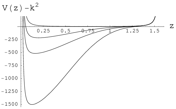
To explore the behavior of the dispersion relations in the large- limit, we now consider the following scaling limit
| (5.15) |
In this limit, the potential (4.22) again greatly simplifies and, consistent with (5.7), becomes
| (5.16) |
This potential is valid in the limit (5.15) for any value of , small or large. If is small, the dispersion relation can be determined using perturbation theory as before, yielding (5.11) without the term. In order to analyze the large- regime, we now consider , and seek to evaluate the dispersion relation as an expansion in . For this purpose, we notice that as the potential (5.16) develops a minimum at
| (5.17) |
as depicted in Fig. 6. The curvature about the minimum is . Thus, if we imagine watching how the wave function changes as we take the large- limit, we will see the wave function getting more and more tightly localized around the point which gets closer and closer to . That is, the wave function will be localized around the tip of the brane . This motivates us to expand the potential around , getting
| (5.18) |
If we now introduce a new variable , the Schrödinger equation (4.21) becomes
| (5.19) |
where
| (5.20) |
and contains only terms that are higher order in :
| (5.21) |
Thus to leading order in the large limit, we can drop the term in (5.19). Upon so doing, and using the expression (5.8) for , the equation (5.19) becomes that of a harmonic oscillator in 4 dimensions with mass and frequency . This quantum mechanics problem can be solved exactly, with wave functions given by
| (5.22) |
up to a normalization constant, and with eigenvalues given by
| (5.23) |
In (5.22), is the generalized Laguerre polynomial of order
| (5.24) |
The allowed values of are determined by the requirement that must be a non-negative integer. The degeneracy of -th energy level is . Higher order corrections in can then be obtained using perturbation theory. For example, with the next order correction included, the degeneracy among states with different and the same is lifted and the eigenvalues are given by
| (5.25) |
with
| (5.26) |
Thus, in the small- limit with fixed and large, we find using (5.20) that the dispersion relation becomes
| (5.27) |
Notice that is negative for the ground state, and indeed for any at sufficiently small . We learn from this calculation that in the large- limit, at low temperatures mesons move with a velocity given to order by . Recalling that to the order we are working , this result can be expressed in terms of , and using (3.32). In the next subsection, we shall obtain the meson velocity at large for any .
5.2 Large- dispersion relation at generic temperature
The technique of the previous subsection can be generalized to analyze the dispersion relation in the large- limit at a generic temperature below the dissociation temperature. For general , one again observes that the potential has a sharper and sharper minimum near the tip of the brane as becomes larger and larger. Thus, in the large limit, we only need to solve the Schrödinger equation near .
To find the potential as a power series in near , we need to know the solution of (3.38) near the tip of the brane at :
| (5.28) |
At small , using the expansion of in (5.28), we find the tortoise coordinate has the expansion
| (5.29) |
Using (5.28) and (5.29) in (4.22), after some algebra we find
| (5.30) |
where
| (5.31) | |||||
| (5.32) | |||||
| (5.33) | |||||
| (5.34) | |||||
| (5.35) |
and where is given by (5.8). We can understand why the leading difference between the potentials and for the mesons and arises in this approximation in the constant terms and as follows. We see from (4.22) that the difference between and comes only from and , which do not enter multiplied by and so cannot affect , or . Furthermore, and are curvature invariants, see (4), and must therefore be smooth as because for Minkowski embeddings the D7 brane is smooth at . This means that and cannot affect the coefficient of in (5.30).
We can now obtain the dispersion relations from the Schrödinger equations with potentials (5.30) as we did in the previous subsection. After making the rescaling , the Schrödinger equation (4.21) takes exactly the form (5.19), with
| (5.36) |
where and are given by (5.31) and (5.32) respectively, and where contains only terms that are subleading in the expansion, and is given by
| (5.37) |
Thus, we find the large- dispersion relation
| (5.38) |
with
| (5.39) |
and
| (5.40) |
Restoring dimensionful quantities in the dispersion relation (5.38), i.e. undoing (3.34), means multiplying the and constant terms by and , respectively.
We can easily obtain an explicit expression for the wave functions themselves if we neglect the , and higher order terms, as the potential (5.30) is then that in the radial wave equation for a four-dimensional harmonic oscillator. To this order, the wave functions are given up to a normalization constant by
| (5.41) |
where, as before, is the order of the generalized Laguerre polynomial .
The dispersion relations (5.38) are the central result of Section 5. We shall analyze (5.38) and discuss its consequences at length in Sections 5.4 and 6. First, however, we close this more technical discussion with a few remarks related to the approximation that we have used to obtain the large- dispersion relations:
- 1.
The wave function is localized at the tip of the brane, near which is the fixed point of the symmetry at which the shrinks to zero size and the fluctuations are fluctuations in . This is the reason why we find a four-dimensional harmonic oscillator.
- 2.
Our approximation is valid for wave functions that are tightly localized near . Evidently, this approximation must break down for mesons with high enough , whose wave functions explore more of the potential. More precisely, if we increase and while keeping fixed and small, the wave functions are peaked at with a width . Or, if we increase and while keeping fixed and small, the wave functions become wider, with oscillations over a range of from near zero to near and hence a wavelength . In either case, our approximation must break down for , since for this large is no longer small and the wave function is no longer localized near .
- 3.
We must ask at what (or, at what ) stringy effects that we have neglected throughout may become important in the dispersion relations for the mesons that we have analyzed. We can answer this question by comparing the length scale over which the meson wave functions that we have computed varies to the string length scale . Considering first the case where is small, we see from (4.18) that the proper distance between the maximum of the wave function at and the tip of the brane at is
(5.42) and the width of the wave function is
(5.43) Stringy effects can be neglected as long as , meaning
(5.44) where in the last expression we have restored the dimensions of using (3.20) and (3.34). (Since at at large , this parametric criterion is the same for as for .) If is large, the wavelength of the wave function should be compared to meaning that is reduced by a factor and stringy effects can be neglected only as long as
(5.45) We can conclude from either (5.44) or (5.45) that we are justified in using the dispersion relation that we have derived in the limit, as long as we take the limit first.66 6 Recall that although the mesons that we have focussed on have masses of order , there are also higher-lying stringy mesonic excitations with masses of order . Requiring to be large is what justifies our neglect of these stringy mesonic excitations, just as it justifies our neglect of stringy corrections to the dispersion relations of the low-lying mesons. Note also that the latter becomes important at an of order the mass of the former.
- 4.
Notice that as (i.e. approaching the critical embedding), both and vanish. Our approximation will therefore break down at the critical embedding. (One way to see this is to note that in the leading terms in (5.30) we will then have zero times infinity, meaning that it is no longer obvious that these are the leading terms.) However, the first order phase transition occurs at , long before this happens.
5.3 Numerical results
We can also obtain the meson wave functions and dispersion relations numerically, without making either a small or a large- approximation. In this subsection we plot a few examples of such results, and compare them to the analytic expressions that we have derived above upon making the large- approximation.
In Fig. 7 we plot the potentials (4.22) and ground state wave functions for those potentials that we have obtained numerically for three values of . Note the changing vertical scale in the plots of ; as increases, deepens. We see that as increases and the potential deepens, the wave function gets more and more localized near and, correspondingly, the expression (5.41) for the wave function that we have derived in the large- limit using the fact that the wave function becomes localized becomes a better and better approximation to the exact wave function.


In Fig. 8 we show dispersion relations obtained numerically for the ground state meson at several values of the temperature. At each , we solve the Schrödinger equation to find the ground state (using the shooting method) and from the eigenvalue we obtain and hence a point on the dispersion relation. By doing this at many ’s, we obtain the curves plotted. We also overlay the linear approximation to the large- dispersion relations that we shall discuss in Sect. 5.4. In Fig. 9, we plot the corresponding group velocities.
5.4 Summary, limiting velocity and dissociation temperature
In this Section we restate our central result for the dispersion relation and then discuss its implications vis à vis a limiting velocity for mesons at a given temperature as well as a limiting temperature below which mesons with a given velocity are found, and above which they are not.
In Section 5.2, we have derived the large- approximation to the meson dispersion relations at any temperature below the dissociation transition. We have checked this result against numerical solutions valid at any in Section 5.3. We begin by restating the analytic result (5.38):
| (5.46) |
where
| (5.47) |
The constant term (which depends on whether we are discussing the or mesons — or — and on the quantum numbers and ) was given in (5.39) and (5.40). In writing the dispersion relation (5.46) we have restored dimensions by undoing the rescaling (3.34). The dimensionful quantity that we had scaled out and have now restored can be written as
| (5.48) |
where we have used (3.23), (3.32) and (3.33). The first factor in (5.48) is a (dimensionful) constant. The quantity appearing in the second, dimensionless, factor is weakly temperature dependent: it can be read from Fig. 2, and is not constant to the degree that the curve in this plot is not a straight line (in the relevant regime , as corresponds to .) Although using dimensionless variables obtained via scaling by the temperature-dependent was very convenient in deriving all our results, in plotting the dispersion relation and group velocity in Figs. 8 and 9 we have instead plotted and in units of , which is a relevant, constant, physical, quantity comparable in magnitude to . In the remainder of this section, we shall analyze (5.46).
In the large- limit, the asymptotic value of the group velocity is given by . This velocity decreases with increasing temperature, and vanishes as on the critical embedding that separates Minkowski and black hole embeddings in Figs. 1 and 2. At the temperature at which the first order dissociation transition occurs, and .
There is a natural explanation within the dual gravity theory for how the asymptotic velocity can arise. Using (3.37), it is easy to show that in (5.47) can also be written as
| (5.49) |
which we see from (3.35) is precisely the local speed of light at the tip of the D7-brane. (The local speed of light is at , and decreases with decreasing , decreasing to at the tip of the D7-brane where and .) Since we have seen that in the large- limit the wave function of the meson fluctuations becomes more and more localized closer and closer to the tip of the D7-brane, this makes it natural that emerges as the asymptotic velocity for mesons with large .
In the low temperature (equivalently, heavy quark) limit, we find (either directly from (5.47) or, initially, in (5.27) in Section 5.1) that
| (5.50) |
Since at small , using (3.32) we have
| (5.51) |
which is precisely the critical velocity (2.7) obtained in [23] from the screening calculation as the velocity above which the potential between two moving quarks of mass cannot be defined. This is the first of two quantitative comparisons that we will be able to make between our present results for meson propagation and results obtained previously via the screening calculation. We see from Fig. 10 that (5.50) works very well where , which is where it was derived (both here and in [22]).

In order to analyze (5.46) beyond the term, it is instructive to rewrite it as a large- approximation to the dispersion relation itself rather than to , yielding
| (5.52) |
in the form we discussed in Section 1. We see that the term linear in in (5.46) yields a constant shift in the meson energies in (5.52). Whereas is independent of , and , the constant term in (5.52) results in evenly spaced dispersion relations for mesons with differing quantum number, separated by
| (5.53) |
which we plot in Fig. 11.

If we neglect the and higher order terms in (5.52), the dispersion relations are the same for mesons and and are independent of . These degeneracies are broken at order , where first appears. We find that the coefficient of in of (5.52) is typically negative: it is negative at all if for any ; it can become positive only if , and are all large enough. When this coefficient is negative, it means that approaches its large- asymptotic behavior (which is a straight line with slope offset by the constant term in (5.52)) from below. This means that at large and means that the group velocity approaches from above at large , as shown in Fig. 9. However, at the group velocity vanishes and . (We have shown this analytically at small in Section 5.1, see (5.11), and our numerical results as in Section 5.3 indicate that this is so at all .) So, as a function of increasing , the group velocity begins at zero, increases to some maximum value that is greater than , and then decreases to as as depicted in Fig. 9.77 7 This behavior is not inconsistent with our identification of with the local speed of light at the tip of the brane: it is only for that the meson wave function is squeezed down to the tip of the brane; at finite , the wave function is peaked where the local speed of light exceeds . Although is not the maximum possible group velocity, it appears that the maximal velocity exceeds only by a small margin. For example, for the ground state meson whose dispersion relations are given in Figs. 8 and 9, we find that , 0.6, and 0.273 for , 0.5, and 0.756 whereas the maximal velocities are 0.896, 0.634 and 0.342, respectively. We shall therefore simplify the following discussion by taking the maximal possible meson velocity at a given temperature to be the limiting velocity , neglecting the slight imprecision that this introduces.
We now wish to compare our results for the limiting meson velocity at a given temperature to the result (2.6) inferred (qualitatively) from the analysis of screening in a hot wind in [23]. We must first convert into , meaning that we must convert from to as discussed in and around Fig. 2. The result is the solid curve in the left panel of Fig. 12, where we have plotted versus . We have derived this curve as a limiting meson velocity at a given temperature. However, it can just as well be read (by asking where it cuts horizontal lines rather than vertical ones) as giving , the temperature below which mesons with a given velocity are found and above which no mesons with that velocity exist. We see that for , the regime where is given by (5.51) and is therefore given by (2.8). In order to compare our result for at all velocities to (2.6), we parametrize our result as
| (5.54) |
In the left panel of Fig. 12 we compare our result (the solid curve) to (5.54) with set to 1, which is of course (2.6). In the right panel, we plot . We see that this function is close to 1 at all velocities, varying between 1.021 at its maximum and 0.924 at . The weakness of the dependence of on is a measure of the robustness with which the simple scaling (2.6) describes our result for the meson dissociation temperature at all velocities.
6 Discussion and Open Questions
We have used the AdS/CFT correspondence to compute the dispersion relation for the heavy “quarkonium” mesons that exist as stable bound states in the strongly coupled plasma of SYM to which heavy fundamental quarks with mass have been added. In Section 4 we have introduced a new, and more geometrical, method of analyzing these mesons that has allowed us, in Section 5, to obtain the dispersion relations at large- analytically in the form (5.52), which we can summarize as in Section 1 by writing
| (6.1) |
We have computed and explicitly and analytically in Section 5, but at present we have no argument that the behavior of these coefficients, which depend on the meson quantum numbers, could teach us lessons that generalize beyond the particular theory in which we have computed them. On the other hand, the limiting large- meson velocity seems to encode much physics that may generalize to meson bound states in other strongly coupled gauge theory plasmas.
- •
Our explicit result is
(6.2) where is related to as in Fig. 2. We see that depends on the temperature (in the combination ) but not on the meson quantum numbers. We see in Figs. 8 and 9 that decreases with increasing temperature, becoming much less than 1 as the temperature approaches , the temperature at which mesons at rest dissociate. We see in these figures that the coefficient in (6.1) can be negative, meaning that the group velocity approaches its large- value from above. Thus, is the limiting meson velocity at large , but the maximal velocity occurs at finite and is slightly larger than . We describe this quantitatively in Section 5, but it is a small effect and in this discussion we shall ignore the distinction between and the maximal velocity.
- •
We find that , which in the gauge theory is the limiting velocity of the mesons that they attain at large , also has a nice interpretation in the dual gravity theory. It is precisely the local velocity of light at the “tip” of the D7-brane, namely where the D7-brane reaches closest to the black hole. This is physically sensible because we have shown that the D7-brane fluctuations — i.e. the mesons in the dual gravity theory — are localized at the D7-brane tip in the large- limit.
- •
At low temperatures or, equivalently, for heavy quarks we find
(6.3) This is precisely, i.e. even including the numerical factor, the criterion for meson dissociation inferred from a completely different starting point in [23]. The logic there was that the screening length that characterizes the potential between a quark and antiquark moving with is shorter than the quark Compton wavelength, meaning that if a quark and antiquark moving with are separated by more than a Compton wavelength, to leading order in they feel no attractive force. By inference, no mesons should exist with . We now see this result emerging by direct calculation of meson dispersion relations, rather than by inference.
- •
We have a result for , the limiting velocity beyond which there are no meson bound states, at all not just at low temperatures, see Fig. 12. We can just as well read this as determining a temperature above which no meson bound states with velocity exist. We find that up to few percent corrections, see Fig. 12, this is given by
(6.4) Once again, this is a result that was previously inferred from analysis of the velocity dependence of the screening length characterizing the potential between a quark and antiquark moving through the plasma [22]. We have now derived this result and the (few percent) corrections to it for the mesons whose dispersion relations we have explicitly constructed. We should also note that it is a slight abuse of terminology to call at a “dissociation” temperature: although it is a temperature above which no mesons with velocity exist, if we imagine heating the plasma through we have not shown that any mesons present therein dissociate — they may simply slow down. The question of what happens in this hypothetical context is a dynamical one that cannot be answered just from the dispersion relations we have analyzed.
- •
As we discussed in Section 2, the result (6.4) can be read as saying that no mesons with velocity exist when the energy density of the strongly coupled plasma exceeds where, up to small corrections,
(6.5) with the energy density at which mesons at rest dissociate. Correspondingly, the low temperature result (6.3) can be written as
(6.6) valid when and is close to 1. Thinking as in [38], we can ask whether the same result holds in other theories. It will be interesting to address this question in -dimensional gauge theories that are in various senses more QCD-like than SYM. At present, however, we have only investigated the -dimensional gauge theories described by D-branes [55] into which fundamental quarks, and hence mesons, have been introduced by embedding a D-brane [56, 48, 49, 29]. The D-branes fill coordinates . The D-brane fills the first of these coordinates , where may be less than or equal to , as well as of the remaining coordinates. In Appendix B, we sketch an investigation of those theories for which . (The case that we have analyzed throughout the rest of this paper is , .) These theories are not conformal for , as their coupling constant has dimension . It is convenient to introduce a dimensionless . We have not repeated our entire construction for the D-D-brane theories. However, we expect that the wave functions for large- mesons will again be localized at the tip of the D-brane, and therefore expect that in these theories will again be given by the local velocity of light at this location. We compute this velocity in Appendix B. Assuming that this is indeed the limiting meson velocity, we find
(6.7) where is given at small by
(6.8) (Relating to beyond the small limit requires solving the embedding equation given in Appendix B.) In these theories, the energy density of the plasma depends on parameters according to [55]
(6.9) and zero-velocity mesons dissociate at some energy density corresponding to where . From these results we notice that at small
(6.10) meaning that the velocity of (6.7) can be written in the form (6.6) for all values of ! In Appendix B, we describe the verification that (6.4) also holds, but only when phrased as in (6.5) in terms of energy density rather than temperature.
Emboldened by these successes, we advocate investigating the consequences that follow from hypothesizing that and mesons in the strongly coupled quark-gluon plasma of QCD propagate with a dispersion relation (6.1) with dropping dramatically as the temperature approaches from below, and with no bound states with velocity possible if given by (6.4). In applying (6.4) to QCD, it is important to scale relative to the for and mesons in QCD itself. The result for the mesons that we have analyzed is surely affected by the fact that they are deeply bound and so should not be used as a guide to quarkonia in QCD. For example, it seems to overestimate for mesons by a factor of 2 or 3. However, as argued in [22, 23] and as we have discussed above, the velocity scaling (6.4) may transcend the detailed meson physics in any one theory and apply to mesonic bound states in any strongly coupled plasma. The successful comparison of our detailed results to this simple scaling form supports this conjecture.
As we have explained at length in Section 1, meson propagation is only one piece of the physics that must be treated in order to understand quarkonium suppression in heavy ion collisions. Introducing the dispersion relation and limiting velocity that we have found into such a treatment is something we leave to the future, instead making only a few qualitative remarks.
First, from the dispersion relations alone we cannot conclude that if a quark-antiquark pair is produced (from an initial hard scattering) with a velocity , with the limiting meson velocity in the plasma of temperature in which the quark-antiquark pair finds itself, then the quark-antiquark pair do not bind into a meson. The reason that we cannot make this inference is that the dispersion relations describe stable mesons with arbitrarily large momentum , making it a logical possibility that a high velocity quark-antiquark pair with arbitrarily high momentum interacts with the medium in some way such as to slow down and lose energy while conserving its momentum, and thus in some way dresses itself into a meson with arbitrarily high momentum , and velocity . That is, since the dispersion relations describe the propagation of mesons with arbitrarily large momentum, by themselves they do not require that quarkonium production is suppressed when the precursor quark-antiquark pair has velocity . Excluding this possibility, allowed by the kinematics, requires some consideration of the dynamics. The heuristic argument of [23] provides guidance: the precursor quark-antiquark pair with do not attract each other and so even though it is kinematically allowed by the meson dispersion relations for them to slow down and form a meson, instead they will propagate independently through the medium. Thus, the -dependent quarkonium suppression pattern proposed in [22], with the production of quarkonium states with higher than the temperature reached in a given heavy ion collision experiment nevertheless becoming suppressed above a threshold transverse momentum at which a quark-antiquark pair with that transverse momentum has velocity , rests upon the dynamical argument of [23]. It is natural that analyzing quarkonium suppression requires consideration of both the precursor quark-antiquark pair and the putative meson, and only the latter is described by the meson dispersion relation. It is then nice to discover that the limiting meson velocity agrees precisely with the velocity at which quark-antiquark pairs can no longer feel a force at order .
We have just argued that the very large- region of the meson dispersion relation is unlikely to be populated in heavy ion collisions. But, whether or not such large- modes are excited, it is clear from Fig. 8 that at temperatures near to mesons at any move much more slowly than they would if they propagated with their vacuum dispersion relation. There are several in-principle-observable signatures of the slow velocity of quarkonium mesons. First, it increases the separation in space long after the collision between those mesons that are produced at the surface of the fireball moving outwards, and hence escape into vacuum promptly, and those which are produced in the center of the plasma and hence move more slowly than if they had their vacuum dispersion relation. An increase in the typical separation of identical mesons because of this slow velocity effect will shift the onset of Bose-Einstein enhancement in the two particle momentum correlation to a lower relative momentum. This simple idea underlies a technique widely used in heavy ion physics and often referred to as Hanbury-Brown Twiss (HBT) two-particle interferometry, in which identical two-particle momentum correlations are used to determine spatio-temporal characteristics of the collision region. For a review, see Ref. [57]. Quarkonium HBT interferometry would thus in principle be able to find signatures of a depressed meson velocity. Second, non-identical two-particle correlation functions are sensitive to whether one particle species is emitted from the medium on average before or after another particle species . Such a difference in average emission times could result, for instance, if the maximal velocities in the dispersion relations for and differ because of their different mass. The analysis of the effect of a difference in average emission times on non-identical two-particle correlation functions can be found in [58]. In principle, this provides a second way of finding signatures of a depressed velocity for those mesons for which the plasma reaches temperatures close to their dissociation temperature.
Quarkonium mesons in the quark-gluon plasma of QCD have nonzero width. In contrast, the mesons we have analyzed at are stable, with zero width. The dispersion relations that we have found have no imaginary part. This is certainly an artifact of the large number of colors and large coupling limits that we have taken throughout. Processes in which one meson decays into two mesons are suppressed by . And, thermal fluctuations which unbind a meson whose binding energy is are suppressed by the Boltzmann factor
| (6.11) |
which at some fixed is nonperturbative in an expansion about infinite . A calculation of the imaginary part of the meson dispersion relations at finite remains for the future, but this simple consideration is enough to be sure that it is nonzero, as is the case in QCD at weak coupling [11]. As soon as the mesons have nonzero width, their slow velocity has a further consequence in the context of heavy ion collisions: because they move more slowly, they spend a longer time in the medium giving the absorptive imaginary part more time to effect the dissociation of the meson than would otherwise be the case.
Our discussion in this Section has highlighted three different avenues of further investigation opened up by our analysis of meson dispersion relations in a strongly coupled gauge theory plasma. The first is the investigation of the phenomenological consequences for and suppression in heavy ion collisions of a dispersion relation of the form (6.1) with (6.4). Second, it appears to us that the most interesting open question about the mesons whose dispersion relations we have analyzed is extending the calculation to finite and analyzing the width of the mesons. And, third, we could gain significant confidence in the application of the lessons we have learned to QCD by repeating our analysis for heavy quark mesons in the plasma of other strongly coupled gauge theories, in particular those with a controlled degree of nonconformality.
Acknowledgments
HL is supported in part by the A. P. Sloan Foundation and the U.S. Department of Energy (DOE) OJI program. HL is also supported in part by the Project of Knowledge Innovation Program (PKIP) of Chinese Academy of Sciences. HL would like to thank KITPC (Beijing) for hospitality during the last stage of this project. This research was supported in part by the DOE Offices of Nuclear and High Energy Physics under grants #DE-FG02-94ER40818 and #DE-FG02-05ER41360.
Appendices
Appendix A General discussion of brane embedding and fluctuations
In this appendix we present a general discussion of brane embedding in a curved spacetime (in the absence of fluxes) and its small fluctuations. We then specialize to the case of D7-branes embedded in the black hole geometry.
A.1 General discussion
Consider a -dimensional brane in a -dimensional target space whose action is
| (A.1) |
where denote the worldvolume coordinates and is the induced metric in the worldvolume
| (A.2) |
Suppose that solves the equations of motion following from (A.1), thus describing an embedding of the brane in the target spacetime. We are interested in understanding the behavior of small fluctuations around . For this purpose, let
| (A.3) |
The action for can then be obtained straightforwardly from (A.1). The resulting action and equations of motion for are, however, not geometrically transparent. This is due to the fact that is the difference between coordinates and thus does not have good properties under coordinate transformations. A more convenient way to parameterize is to use the exponential map to express it in terms of a vector in the tangent space at , as we now describe. (Such techniques have also been used in the calculation of string worldsheet beta functions [59].) Given a vector , we shoot out geodesics of unit affine parameter from with tangent . The end point of such a geodesic is identified with . Such a map should be one-to-one within a small neighborhood of . To second order in one may solve the geodesic differential equation, finding
| (A.4) |
Note that the appearance of is consistent with the coordinate dependence of ; they can both be shown to have the same variation under a coordinate transformation.
Using the parametrization (A.4), we find that
| (A.5) | ||||
with
| (A.6) |
The simplest way to find (A.5) is to use the Riemann Normal coordinates at in which the Christoffel symbols vanish. is the induced metric in the worldvolume theory and below indices will be raised and lowered by . To quadratic order in we have
| (A.7) |
We now take to be orthogonal to the brane worldvolume (which corresponds to choosing the static gauge), i.e.
| (A.8) |
where are unit vectors orthogonal to the worldvolume direction. Note that and together span the full tangent space at . i.e.
| (A.9) |
and
| (A.10) |
We now introduce
| (A.11) |
is the extrinsic curvature of the brane in the -direction, and is symmetric in . (This follows from the fact that a surface orthogonal to satisfies for some one-form . Note also that can be written as , where is the Lie derivative along -direction.) , which is antisymmetric in , is an connection for the transverse directions. Note that the choice of (and thus ) is not unique. One can choose a different set of basis vectors by making an arbitrary local transformation. Thus transforms as a vector under the “gauge” symmetry and transform as a connection. Note that this gauge symmetry is not dynamical. With these definitions we can now write
| (A.12) |
where
| (A.13) |
is an covariant derivative. Using (A.12) in (A.1), we now find that
| (A.14) |
with . For to satisfy the equations of motion, the terms in (A.14) that are linear in the ’s have to vanish. This implies that
| (A.15) |
These are the embedding equations for the background. Thus, the action (A.14) for the small fluctuations to quadratic order becomes
| (A.16) |
We have used both the embedding equations (A.15) and the action for the small fluctuations (A.16) in Section 4.
The action (A.16) can be further simplified if satisfies additional constraints. For example, if is proportional to a Killing vector, then
| (A.17) |
This follows from the fact that satisfies for some . If in addition is a hypersurface orthogonal, i.e. if it satisfies for some one form , then
| (A.18) |
We have used this simplification in Section 4.
Finally, note that equation (A.16) was written using the coordinate split (A.9). One can write it and other equations in a more covariant way by introducing
| (A.19) |
and using these objects in place of and in various places. is the covariant induced metric on the brane and is the projector onto the worldvolume directions.
A.2 D7-branes in black hole
We now specialize to the case of D7-branes considered in the main text, where we have two transverse directions with
| (A.20) |
where are normalization factors. In this case is proportional to the two-dimensional antisymmetric tensor . It is easy to see that is both hypersurface orthogonal and proportional to a Killing vector (since nothing depends on ). We thus have and . The action (A.16) now reduces to the form we have used in Section 4, namely
| (A.21) |
where the “masses” are given by
| (A.22) | |||||
| (A.23) |
with , and as defined in (4). In writing (A.21)–(A.23) we have used the identities
| (A.24) |
and the fact that for the black hole spacetime. We can also use the generalization of the Gauss-Codazzi relation for a codimension two surface which we derive in Section A.3, see Eq. (A.28), to write
| (A.25) |
Therefore, in (A.22) can equivalently be written as
| (A.26) |
which is the form that we used in Section 4.
A.3 Gauss-Codazzi relations for co-dimension 2
Define the covariant derivative on the D7 brane as
| (A.27) |
This is equivalent to the covariant derivative defined with respect to . We can now use to define the curvature of the D7-brane and then relate it to the curvature of the full space. Calculations similar to those in [60] reveal that
| (A.28) |
where labels the two directions perpendicular to the brane and is summed over. is the projection of the full Riemann tensor onto the D7-brane,
| (A.29) |
Taking further contractions of Eq. (A.28) with and and using Eq.(A.10) gives
| (A.30) |
where are both summed. In the case of interest, where because is proportional to a Killing vector and where is the embedding equation, we obtain (A.25).
Appendix B D-D-Brane Theories
It will be of interest in future to study the degree to which the meson dispersion relations that we have derived, together with their consequences like (6.3) and (6.4), change as one modifies the gauge theory to make it more QCD-like. In this appendix, we report on a check that we have mentioned in Section 6 in which the gauge theory is modified, albeit not in the direction of QCD. We consider the -dimensional gauge theories described by D-branes [55] into which fundamental quarks, and hence mesons, have been introduced by embedding D-branes [56, 48, 49, 29]. The D-branes fill coordinates . The D-branes fill coordinates , where , as well as of the remaining coordinates. In the large- limit, the near horizon geometry of the D-branes is dual to a -dimensional supersymmetric Yang-Mills theory with 16 supercharges that is nonconformal for . We will restrict to . In the approximation, the D-branes live in the background D-brane geometry, and their back-reaction on the geometry can be neglected. Strings which stretch between the D- and the D-branes are dual to fundamental quarks in the gauge theory. We shall set . And, scalar mesons in the gauge theory are represented by fluctuations of the position of the Dq-brane. The specific case that we have analyzed throughout most of this paper is , . In this more general setting, as in the specific case, there is a dissociation transition at some at which the spectrum of meson fluctuations changes from discrete to continuous.
The background D-brane geometry is described by the metric [55]
| (B.1) |
and the dilaton
| (B.2) |
where
| (B.3) | |||||
| (B.4) | |||||
| (B.5) |
and where we are using dimensionless coordinates as in (3.35). The black hole horizon is located at . specifies the position where the D-brane that we introduce will sit, as follows. We shall embed a D-brane described, in the absence of fluctuations, by a curve with the D-brane placed such that its tip is located at and , and then use to rescale metric coordinates such that the tip of the D-brane is at . After this rescaling, the metric and dilaton are given by (B.1) and (B.2). The holographic dictionary determines the coupling, number of colors, and temperature in the gauge theory via
| (B.6) | |||||
| (B.7) | |||||
| (B.8) |
Note that has dimension , making it useful to define the dimensionless coupling
| (B.9) |
The differential equation that specifies the shape of the embedding curve can be derived as we did in obtaining (3.31). For the special case in which , the embedding equation simplifies, becoming
| (B.10) |
We have scaled our variables so that the tip of the D-brane is at ; in order to have a smooth embedding we require ; using these boundary conditions, we can then solve the embedding equation and obtain , which defines via , . Finally, we can determine what the mass of the quarks that we are analyzing is via
| (B.11) |
From (B.6), (B.8) and (B.11) we find that
| (B.12) |
where the constant is given by
| (B.13) |
We also note that the energy density of the plasma is given by [55]
| (B.14) |
where the constant is given by
| (B.15) |
This means that
| (B.16) |
where the zero-velocity mesons dissociate at a temperature corresponding to and , with a constant of order unity.
We shall not repeat our construction of the meson wave functions and dispersion relations for the D-D system here. Instead, we shall assume that in the large- limit the meson wave functions become localized at the tip of the D brane at and , as we found for the D3-D7 system. As a consequence, the limiting meson velocity will be given by the local speed of light at the tip of the D-brane. This velocity can be read from the metric (B.1), and is given by
| (B.17) |
In Section 6 we have analyzed this result in the small limit, showing that in this limit it takes on the form (6.6) for any . This illustrates the generality of the result (6.3) when it is phrased in terms of the energy density. Here, we shall analyze (B.17) at arbitrary , seeking to compare it to (6.4). From (B.17) and (B.16) we see that the critical velocity satisfies
| (B.18) |
Recall that is a constant of order unity and that is a weak function of temperature and hence of , obtained by solving the embedding equation and making a plot of vs. as in Fig. 2, and reading off the ratio.
Much as we did in Section 6, we can see (B.18) either as giving the limiting velocity as a function of , or as giving , the energy density above which no mesons with velocity exist, via
| (B.19) |
This is the generalization of (6.4) to the D-D system. It is written somewhat implicitly, since which occurs within the square brackets is a weak function of . It is nevertheless manifest that the entire expression in the square brackets is a weak function of , varying from one constant of order one at to some different constant of order one at . As in (5.54), we can then define a function by rewriting (B.19) as
| (B.20) |
where is the Lorentz boost factor. Equivalently, using (B.14) we can write
| (B.21) |
We have seen in Fig. 12 that for the D3-D7 brane system, is everywhere close to , with being the farthest it gets from 1. We have also done the exercise of solving the embedding equations for , the D4-D6 brane system with , and find in that case that the farthest that gets from is .
Given its derivation via (B.18), it would have been reasonable to try writing
| (B.22) |
instead of (B.20). This does not work as well, yielding a that reaches 1.306 for the D3-D7 system and 1.261 for the D4-D6 system. So although there is no important parametric difference between (B.22) and (B.20), we have focussed on the form (B.20), and hence (B.21), throughout this paper.
The most important conclusion from our D-D investigation in this Appendix comes by comparing (B.20) and (B.21). We see that in all the D-D systems we analyze, the leading velocity dependence of is that it is proportional to , as if the mesons see a boosted energy density as we discussed in Section 2. In contrast, scales with a power of that depends on .
References
- [1] T. Matsui and H. Satz, Phys. Lett. B 178, 416 (1986).
- [2] For a review, see H. Satz, J. Phys. G 32 (2006) R25 [arXiv:hep-ph/0512217].
- [3] J. Kuti, J. Polonyi and K. Szlachanyi, Phys. Lett. B 98 (1981) 199; L. D. McLerran and B. Svetitsky, Phys. Lett. B 98 (1981) 195; L. D. McLerran and B. Svetitsky, Phys. Rev. D 24 (1981) 450; O. Kaczmarek, F. Karsch, P. Petreczky and F. Zantow, Phys. Lett. B 543 (2002) 41 [arXiv:hep-lat/0207002].
- [4] O. Kaczmarek, F. Karsch, F. Zantow and P. Petreczky, Phys. Rev. D 70, 074505 (2004) [Erratum-ibid. D 72, 059903 (2005)] [arXiv:hep-lat/0406036].
- [5] P. Petreczky and K. Petrov, Phys. Rev. D 70 (2004) 054503 [arXiv:hep-lat/0405009].
- [6] O. Kaczmarek and F. Zantow, Phys. Rev. D 71, 114510 (2005) [arXiv:hep-lat/0503017].
- [7] Y. Maezawa, S. Ejiri, T. Hatsuda, N. Ishii, N. Ukita, S. Aoki and K. Kanaya, PoS LAT2006, 141 (2006) [arXiv:hep-lat/0610013].
- [8] For a review, see F. Karsch, Nucl. Phys. A 783, 13 (2007) [arXiv:hep-ph/0610024].
- [9] M. Asakawa, T. Hatsuda and Y. Nakahara, Prog. Part. Nucl. Phys. 46 (2001) 459 [arXiv:hep-lat/0011040]; T. Umeda, R. Katayama, O. Miyamura and H. Matsufuru, Int. J. Mod. Phys. A 16 (2001) 2215 [arXiv:hep-lat/0011085]; T. Umeda, K. Nomura and H. Matsufuru, Eur. Phys. J. C 39S1, 9 (2005) [arXiv:hep-lat/0211003]; M. Asakawa and T. Hatsuda, Phys. Rev. Lett. 92, 012001 (2004) [arXiv:hep-lat/0308034]; S. Datta, F. Karsch, P. Petreczky and I. Wetzorke, Phys. Rev. D 69, 094507 (2004) [arXiv:hep-lat/0312037]; H. Iida, T. Doi, N. Ishii and H. Suganuma, PoS LAT2005 (2006) 184 [arXiv:hep-lat/0509129]; A. Jakovac, P. Petreczky, K. Petrov and A. Velytsky, Phys. Rev. D 75, 014506 (2007) [arXiv:hep-lat/0611017].
- [10] R. Morrin et al., PoS LAT2005, 176 (2005) [arXiv:hep-lat/0509115]; G. Aarts et al., PoS LAT2006, 126 (2006) [arXiv:hep-lat/0610065]; G. Aarts et al., arXiv:0705.2198 [hep-lat]; M. B. Oktay et al., arXiv:0710.2795 [hep-lat].
- [11] M. Laine, O. Philipsen, P. Romatschke and M. Tassler, JHEP 0703, 054 (2007) [arXiv:hep-ph/0611300]; M. Laine, JHEP 0705, 028 (2007) [arXiv:0704.1720 [hep-ph]]; M. Laine, O. Philipsen and M. Tassler, JHEP 0709, 066 (2007) [arXiv:0707.2458 [hep-lat]]; Y. Burnier, M. Laine and M. Vepsalainen, arXiv:0711.1743 [hep-ph].
- [12] F. Karsch, D. Kharzeev and H. Satz, Phys. Lett. B 637, 75 (2006) [arXiv:hep-ph/0512239].
- [13] B. Alessandro et al. [NA50 Collaboration], Eur. Phys. J. C 39, 335 (2005) [arXiv:hep-ex/0412036]; R. Arnaldi et al. [NA60 Collaboration], Nucl. Phys. A 783 (2007) 261 [arXiv:nucl-ex/0701033]. A. Adare et al. [PHENIX Collaboration], Phys. Rev. Lett. 98 (2007) 232301 [arXiv:nucl-ex/0611020].
- [14] F. Carminati et al. [ALICE Collaboration], J. Phys. G 30, 1517 (2004); B. Alessandro et al. [ALICE Collaboration], J. Phys. G 32, 1295 (2006); D. d’Enterria et al. [CMS Collaboration], J. Phys. G 34, 2307 (2007).
- [15] K. Adcox et al. [PHENIX Collaboration], Nucl. Phys. A 757 (2005) 184 [arXiv:nucl-ex/0410003]; B. B. Back et al. [PHOBOS Collaboration], Nucl. Phys. A 757 (2005) 28 [arXiv:nucl-ex/0410022]; I. Arsene et al. [BRAHMS Collaboration], Nucl. Phys. A 757 (2005) 1 [arXiv:nucl-ex/0410020]; J. Adams et al. [STAR Collaboration], Nucl. Phys. A 757 (2005) 102 [arXiv:nucl-ex/0501009].
- [16] J. W. Qiu, Nucl. Phys. A 783 (2007) 309 [arXiv:nucl-th/0610128].
- [17] J. W. Qiu, J. P. Vary and X. f. Zhang, Phys. Rev. Lett. 88 (2002) 232301 [arXiv:hep-ph/9809442].
- [18] D. Kharzeev and K. Tuchin, Nucl. Phys. A 770 (2006) 40 [arXiv:hep-ph/0510358].
- [19] R. L. Thews, M. Schroedter and J. Rafelski, Phys. Rev. C 63 (2001) 054905 [arXiv:hep-ph/0007323]; L. Grandchamp and R. Rapp, Phys. Lett. B 523 (2001) 60 [arXiv:hep-ph/0103124]; A. Andronic, P. Braun-Munzinger, K. Redlich and J. Stachel, Phys. Lett. B 571 (2003) 36 [arXiv:nucl-th/0303036].
- [20] F. Karsch and R. Petronzio, Z. Phys. C 37, 627 (1988).
- [21] M. C. Chu and T. Matsui, Phys. Rev. D 39, 1892 (1989).
- [22] H. Liu, K. Rajagopal and U. A. Wiedemann, Phys. Rev. Lett. 98, 182301 (2007) [arXiv:hep-ph/0607062].
- [23] H. Liu, K. Rajagopal and U. A. Wiedemann, JHEP 0703, 066 (2007) [arXiv:hep-ph/0612168].
- [24] S. J. Brodsky and A. H. Mueller, Phys. Lett. B 206 (1988) 685; S. Gavin, M. Gyulassy and A. Jackson, Phys. Lett. B 207 (1988) 257; N. Armesto and A. Capella, Phys. Lett. B 430 (1998) 23 [arXiv:hep-ph/9705275].
- [25] D. Kharzeev and H. Satz, Phys. Lett. B 334 (1994) 155 [arXiv:hep-ph/9405414]; S. G. Matinyan and B. Muller, Phys. Rev. C 58 (1998) 2994 [arXiv:nucl-th/9806027]; L. Maiani, F. Piccinini, A. D. Polosa and V. Riquer, Nucl. Phys. A 741 (2004) 273 [arXiv:hep-ph/0402275].
- [26] D. Kharzeev and H. Satz, Phys. Lett. B 356 (1995) 365 [arXiv:hep-ph/9504397].
- [27] S. S. Adler et al. [PHENIX Collaboration], Phys. Rev. Lett. 96 (2006) 012304 [arXiv:nucl-ex/0507032].
- [28] Beginning with G. Policastro, D. T. Son and A. O. Starinets, Phys. Rev. Lett. 87, 081601 (2001) [arXiv:hep-th/0104066].
- [29] D. Mateos, R. C. Myers and R. M. Thomson, JHEP 0705, 067 (2007) [arXiv:hep-th/0701132].
- [30] J. M. Maldacena, Adv. Theor. Math. Phys. 2, 231 (1998) [Int. J. Theor. Phys. 38, 1113 (1999)] [arXiv:hep-th/9711200]; E. Witten, Adv. Theor. Math. Phys. 2, 253 (1998) [arXiv:hep-th/9802150]; S. S. Gubser, I. R. Klebanov and A. M. Polyakov, Phys. Lett. B 428, 105 (1998) [arXiv:hep-th/9802109]; O. Aharony, S. S. Gubser, J. M. Maldacena, H. Ooguri and Y. Oz, Phys. Rept. 323, 183 (2000) [arXiv:hep-th/9905111].
- [31] S. J. Rey and J. T. Yee, Eur. Phys. J. C 22, 379 (2001) [arXiv:hep-th/9803001].
- [32] J. M. Maldacena, Phys. Rev. Lett. 80, 4859 (1998) [arXiv:hep-th/9803002].
- [33] S. J. Rey, S. Theisen and J. T. Yee, Nucl. Phys. B 527, 171 (1998) [arXiv:hep-th/9803135]; A. Brandhuber, N. Itzhaki, J. Sonnenschein and S. Yankielowicz, Phys. Lett. B 434, 36 (1998) [arXiv:hep-th/9803137]; J. Sonnenschein, arXiv:hep-th/0003032.
- [34] D. Bak, A. Karch and L. G. Yaffe, JHEP 0708, 049 (2007) [arXiv:0705.0994 [hep-th]].
- [35] I. Amado, C. Hoyos-Badajoz, K. Landsteiner and S. Montero, JHEP 0709, 057 (2007) [arXiv:0706.2750 [hep-th]].
- [36] K. Peeters, J. Sonnenschein and M. Zamaklar, Phys. Rev. D 74, 106008 (2006) [arXiv:hep-th/0606195]; M. Chernicoff, J. A. Garcia and A. Guijosa, JHEP 0609, 068 (2006) [arXiv:hep-th/0607089]; see also Appendix A of C. P. Herzog, A. Karch, P. Kovtun, C. Kozcaz and L. G. Yaffe, JHEP 0607, 013 (2006) [arXiv:hep-th/0605158].
- [37] S. D. Avramis, K. Sfetsos and D. Zoakos, Phys. Rev. D 75, 025009 (2007) [arXiv:hep-th/0609079].
- [38] E. Caceres, M. Natsuume and T. Okamura, JHEP 0610, 011 (2006) [arXiv:hep-th/0607233].
- [39] M. Natsuume and T. Okamura, JHEP 0709, 039 (2007) [arXiv:0706.0086 [hep-th]].
- [40] F. Karsch, E. Laermann and A. Peikert, Phys. Lett. B 478, 447 (2000) [arXiv:hep-lat/0002003]; F. Karsch, Nucl. Phys. A 698, 199 (2002) [arXiv:hep-ph/0103314].
- [41] A. Karch and E. Katz, JHEP 0206, 043 (2002) [arXiv:hep-th/0205236].
- [42] M. Kruczenski, D. Mateos, R. C. Myers and D. J. Winters, JHEP 0307, 049 (2003) [arXiv:hep-th/0304032].
- [43] J. Babington, J. Erdmenger, N. J. Evans, Z. Guralnik and I. Kirsch, Phys. Rev. D 69, 066007 (2004) [arXiv:hep-th/0306018].
- [44] M. Kruczenski, D. Mateos, R. C. Myers and D. J. Winters, JHEP 0405, 041 (2004) [arXiv:hep-th/0311270].
- [45] S. Hong, S. Yoon and M. J. Strassler, JHEP 0404, 046 (2004) [arXiv:hep-th/0312071].
- [46] I. Kirsch, Fortsch. Phys. 52, 727 (2004) [arXiv:hep-th/0406274].
- [47] I. Kirsch and D. Vaman, Phys. Rev. D 72, 026007 (2005) [arXiv:hep-th/0505164].
- [48] R. C. Myers and R. M. Thomson, JHEP 0609, 066 (2006) [arXiv:hep-th/0605017].
- [49] D. Mateos, R. C. Myers and R. M. Thomson, Phys. Rev. Lett. 97, 091601 (2006) [arXiv:hep-th/0605046].
- [50] C. Hoyos, K. Landsteiner and S. Montero, JHEP 0704, 031 (2007) [arXiv:hep-th/0612169].
- [51] R. C. Myers, A. O. Starinets and R. M. Thomson, arXiv:0706.0162 [hep-th].
- [52] K. Peeters and M. Zamaklar, arXiv:0711.3446 [hep-th].
- [53] J. Erdmenger, N. Evans, I. Kirsch and E. Threlfall, arXiv:0711.4467 [hep-th].
- [54] See Eqs. 22.7.1-3 in M. Abramowitz and I. A. Stegun, eds., Handbook of Mathematical Functions, U.S. Government Printing Office, Washington, DC,1964.
- [55] N. Itzhaki, J. M. Maldacena, J. Sonnenschein and S. Yankielowicz, Phys. Rev. D 58, 046004 (1998) [arXiv:hep-th/9802042].
- [56] D. Arean and A. V. Ramallo, JHEP 0604, 037 (2006) [arXiv:hep-th/0602174].
- [57] M. A. Lisa, S. Pratt, R. Soltz and U. Wiedemann, Ann. Rev. Nucl. Part. Sci. 55, 357 (2005) [arXiv:nucl-ex/0505014].
- [58] R. Lednicky, V. L. Lyuboshits, B. Erazmus and D. Nouais, Phys. Lett. B 373 (1996) 30.
- [59] For a review, see C. G. Callan and L. Thorlacius, in Particles, strings and supernovae: proceedings of TASI Institute in Elementary Particle Physics, A. Jevicki and C.-I. Tan, eds. (Worlds Scientific: 1989).
- [60] See Chapter 10 and in particular Eq. (10.2.23) in R. M. Wald, General Relativity, (University of Chicago Press, 1984).