Indirect control with quantum accessor: coherent control by initial state preparation

Quantum control is a coherent manipulation of a quantum system, which enables a time evolution from an arbitrary initial state to arbitrarily given target states Tarn; book1; book2; book3; Warren1993; rabitz1996; viola1999; rabitz2000; lloyd2000; roa; tarn2007. Recently, we proposed the conception of indirect quantum control(IDQC) xue; ind3. A similar work under the name of incoherent quantum control ind1; ind2; ind4 was proposed by R. Roman et.al. for the control of spin-half particles. The IDQC is a coherent manipulation for a quantum system via a coupled intermediate system (called quantum accessor), which can be controlled directly. Through the engineered interaction between the controlled quantum system and the accessor, this indirect manipulation enable an ideal control of the system. A similar controllability for incoherent control Tarn has been studied in the $SU(2)\otimes SU(2)$ case that both the controlled system and quantum accessor are spin-$1/2$ particles ind1; ind2.

Our first paper ind3 on indirect quantum control was motivated by the pervious works on the quantum control with built-in feedback xue and on the dipole control for finite quantum systems fu1; fu2. In Ref. ind3, a general indirect quantum control protocol is proposed and studied in detail with an engineered interaction totally fixed between the controlled quantum system and the accessor. In this scheme the accessor is modeled as a qubit chain with XY-type coupling. Conditions for the complete controllability, such as the minimal number of qubits in accessor, the coupling way between the system and the accessor, are investigated in detail.

Different from the scheme proposed in Ref. ind3, the quantum control scheme proposed in this paper is mainly based on ingeniously preparing the initial state of the quantum “$\emph{accessor}$”. In this scheme, the control function is encoded in a series of initial states of the accessor, which is prepared by means of a classical field, and realized through the conditional evolution of the controlled system from the initial states. So it is adequate to say that this is essentially an indirect control protocol where the initial preparation of the “quantized accessor” determines the time evolution of the controlled system to realize the target state.

In this paper, we assume that the interaction which governs the evolution of the controlled system depends on the initial state of the accessor, and it is switched off when the external field is switched on to manipulate the accessor. This “switch off and on duality” can be approximately realized when the strength of the external field is much stronger than the system-accessor coupling. Actually, in physical situations it is rather difficult to control the system state directly, but it is easy to manipulate the accessor state and modify the $\emph{system}$ state by switching on and off the interaction between them. We will only consider the quantum controllability of finite dimensional systems, and leave the relevant infinite case Tarn-infinite as an open problem.

The remainder of this paper is organized as follows. In Sec. II, we describe in detail the control steps of our IDQC scheme by a model. In Sec. III, we generally investigate the controllability, in a slightly generalized sense, of the scheme along the line of Ref. jurdjeiv. In Sec. IV, we consider explicitly an example to illustrate the IDQC scheme and the concerned controllability.

Let the controlled system $S$ be a finite-level system described by the Hamiltonian $H_{S}$ and the quantum accessor $A$ be a high-dimension system described by the Hamiltonian $H_{A}$. In our scheme the control process is steered by the preparation of the initial states of $A$. To realize the conditional evolution of the system, we require the interaction $H_{I}(S,A)$ between the system and the accessor commute with $H_{A}$, i.e., $\left[H_{A},H_{I}\left(S,A\right)\right]=0$. Thus the Hamiltonian of the total system of $S$ and $A$ can be written as

We observe that in our model $H_{A}$ commutes with both $H_{S}$ and $H_{I}(S,A)$. Actually, in the “standard” approach for ideal quantum measurement, we require a non-demolition property, defined by the above commutation relations. Here we can imagine the controlled system as a detector, which will not dissipate the energy of the accessor, but on the other hand can record the manipulation information of the accessor. Then the evolution of the controlled system is steered by the quantum states of $A$. The interaction Hamiltonian $H_{I}(S,A)$ between the two subsystems enjoys the following nice property. For the fixed variable of the controlled system, which can be viewed as the classical parameter, the operator $H_{A}$ and $H_{I}\left(S,A\right)$ have the common eigenstates $|\phi_{j}\rangle$ because of the commutating relation. The corresponding eigenvalues $H_{j}\left(S\right)$ are parameterized by the variables of the controlled system and thus can be regarded as an operator acting on the Hilbert space of the controlled system. Thus for each eigenstate $|\phi_{j}\rangle$ of the accessor and an arbitrary state $|\psi\rangle$ of the system,

where $H_{j}(S)$ is an operator acting on the state space of $S$ and depends on the initial eigenstate of the accessor. In this sense, we regard $H_{j}\left(S\right)$ as an effective Hamiltonian acting on the controlled system.

Actually for an arbitrary initial state $|\psi_{0}\rangle$ of $S$ and an eigenstate $|\phi_{j}\rangle$ Hamiltonian $H_{A}$ of the accessor $A$ with eigenvalue $\alpha_{j}$, we have

This means that different initial states of the accessor can induce different time evolutions of the controlled system, which are defined by the effective Hamiltonian

Therefore the different effective Hamiltonian $H_{\text{{\scriptsize eff}}}\left(j\right)$ can be induced by preparing the different initial states of the accessor. The above simple observations motivate us to propose a new IDQC scheme. In our control scheme, we assume that we can manipulate the accessor $A$ to any common eigenstate state of $H_{A}$ and $H_{I}(S,A)$. The system is manipulated by the series of effective Hamiltonians $\{H_{\text{{\scriptsize eff}}}\left(j\right)\}$ induced by preparing different initial states of the accessor. Here, we take the model Hamiltonian as

where $E\left(t\right)$ depends on the variables $Y_{j}$ of the accessor and $u_{j}\left(t\right)$ is the external field used to prepare the initial states of the accessor. We assume that $u_{j}\left(t\right)$ is so strong that the system-accessor coupling can be ignored when the external field is switched on. Therefore, we can formally use the “step” function $f\left(t\right)$ to describe the periodic control scheme. Fig. 1 illustrates this “switch on-off” duality control scheme. Here the basic element is what we call control cycle (Dashed rectangular area in Fig. 1) consisting of the following two steps:

1. S1.

   In the time interval $\left(t_{1}^{\prime},t_{1}\right)$, the interaction is broken between the accessor and the controlled system, $f\left(t\right)=0$, and the accessor is prepared on the state $|\phi_{j_{1}}\rangle$ with the classical field $E\left(t\right)$.

2. S2.

   In the time interval $\left(t_{1},t_{2}^{\prime}\right)$, the interaction between $S$ and $A$ is switched on $f\left(t\right)\neq 0$ and the classical field is removed. In this step, the system evolves according to the effective Hamiltonian $H_{\text{{\scriptsize eff}}}\left(j\right)$. The encoding control information is “recorded” by the system and we finish one cycle of manipulation.

In our scheme, the controllability is realized by repeating this cycle.

In this section, we consider the complete controllability of the controlled system $S$ with the above indirect scheme. For simplicity, we only consider the case where the controlled system $S$ is an $N$-level system. To explore the controllability, we define the set of discrete evolution operators

each element of which represents a manipulation completed in $M$ control cycles. In the $jth$ cycle, the interaction between $S$ and $A$ is switched on for $\Delta t_{j}$. The set of attainable states from the state $\phi_{0}$ is

where $|\phi_{0}\rangle$ is the initial state of the controlled system. By definition, $\mathcal{G}$ is a semigroup and a subset of the Lie group $SU(N)$. Mathematically, the subsystem $S$ is completely controllable if $\mathcal{G}$ is the whole Lie group $SU(N)$. However, physically speaking, this condition is by far too strong. It would be well acceptable to call $S$ completely controllable if an arbitrary state of $S$ can be approached by the state in $\mathcal{G}_{\phi_{0}}$ to an arbitrary precision. This latter condition means that the closure $\mathcal{\bar{G}}$ of $\mathcal{G}$ in $SU(n)$ is just $SU(N)$ itself. In view of this consideration, we will investigate $\mathcal{\bar{G}}$.

As far as complete controllability is concerned it is meaningful to investigate under what conditions $\mathcal{\bar{G}}$ is equal to $SU(N)$. To this end we need to go into the details of $H_{S}$ and $H_{j}(S)$. But we will content ourself with considering a special case, which illustrates the main idea. We assume that for each $j$ the Hamiltonian $H_{j}(S)$ takes the form $H_{j}(S)=\lambda(\alpha_{j})X_{j}$, where $\alpha_{j}$ is a parameter that can be manipulated freely to enable $\lambda(\alpha_{j})$ to take zero or some real fixed number. For convenience, the model with this property will be referred to as the simplified model. And $|\lambda(\alpha_{j})|$ can be arbitrarily large, if necessarily. This fact turns out to be crucial for the complete controllability.

Under the above assumption, the effective Hamiltonian reads

This is exactly the Hamiltonian broadly discussed in the direct quantum control jurdjeiv; Tarn. But here it appears naturally in our scheme. So in some sense it can be said that the scheme proposed in this paper is at the bottom of the broadly discussed direct quantum control scheme. Especially, the method of controllability proving developed in direct quantum control theory applies in our present case.

The following two lemmas are essentially taken from Ref. jurdjeiv. We would rather omit the proof. But we would like to point out that in the proof of Lemma 2 the condition ”$|\lambda(\alpha_{j})|$ can be arbitrarily large, if necessarily” plays a crucial role.

Proof. Denote by $\mathcal{L}$ the Lie algebra of $\mathcal{\bar{G}}$, which is a Lie subgroup of $SU(N)$ according to Lemma 1. It directly follows from Lemma 2 that $iX_{j}\in\mathcal{L}$ for each $j$. On the other hand for $\Delta t_{j}\geq 0$

by definition. But $\mathcal{\bar{G}}$ is a group, this should be true for an arbitrary $\Delta t_{j}$. Consequently, we have $-i(H_{S}+\lambda(\alpha_{j})X_{j})\in\mathcal{L}$, and hence $iH_{S}\in\mathcal{L}$. Finally, as $iH_{S}$ and $iX_{j}$’s generate the Lie algebra $su(N)$ and $SU(N)$ is a connected Lie group we can conclude that $\mathcal{\bar{G}}=SU(N)$. The proof of the proposition is thus completed.

We have proved the controllability of the simplified model. In this model, the control is attained by repeatedly and properly preparing the initial states of the accessor and the controlled system works as a detector, which records and reads the manipulation information encoded in the initial states of the accessor. This is also the main idea of the IDQC proposed in this paper.

In this section, we illustrate the above control scheme and its controllability with an example: a two-level accessor controls one qubit. In this simple example, we show that the scheme is equivalent to that of the direct quantum control.

Let the controlled system be a qubit described by the Hamiltonian $H_{S}=\omega_{S}\sigma_{S}^{z}$ and the accessor be a two-level system with the free Hamiltonian $H_{A}=\omega_{A}\sigma_{A}^{z}$. We couple the controlled system and the accessor with the interaction $H_{I}=g\sigma_{S}^{x}\otimes\sigma_{A}^{z}$. Thus the total Hamiltonian of the system reads

It is easily seen that if the initial state of the accessor is $|0\rangle$, the effective Hamiltonian defined above reads

If the initial state of accessor is $|1\rangle$, we obtain the effective Hamiltonian

This effective Hamiltonian is equivalent to the Hamiltonian of a qubit controlled by a transverse magnetic field the direction of which can be reversed.

Obviously, we have $i\sigma_{S}^{x}\in su\left(2\right)$, $i\sigma_{S}^{z}\in su\left(2\right)$ and $i\sigma_{S}^{y}=\left[i\sigma_{S}^{x},i\sigma_{S}^{z}\right]/2i\in su\left(2\right)$, producing the generators of the Lie algebra $SU\left(2\right)$. Thus when $g>>\omega_{S}$ Proposition 1 applies and we conclude that the system is controllable.

Next, we would follow the controlling process step by step. The time evolution operator of the controlled system is calculated straightforward as

where $\Omega=\sqrt{\omega_{S}^{2}+g^{2}}$ and $\hat{\varphi}=\omega_{A}\sigma_{A}t$. Suppose that the initial state of $S$ is $\left|0\right\rangle_{S}$. First we close the interaction by taking $g=0$ and use the classical field to prepare the accessor $A$ in the initial state $\left|0\right\rangle_{A}$. Then we stop the action of the classical field and switch on the interaction. Driven by the effective Hamiltonian $H_{\text{{\scriptsize eff}}}\left(0\right)$ for the time interval $t_{1}$, the quantum state of the controlled system becomes

where $\alpha\left(t_{1}\right)=\left(\cos\Omega t_{1}+i\frac{\omega_{S}}{\Omega}\sin\Omega t_{1}\right)$ and $\beta\left(t_{1}\right)=i\frac{g}{\Omega}\sin\Omega t_{1}$. Noticing that the wave function of the total system remains factorized, we obtain the state of the controlled system after the evolution as

In this equation , when $g>>\omega_{S}$, we obtain $\alpha\left(t_{1}\right)\approx\cos\Omega t_{1}$ and $\beta\left(t_{1}\right)\approx i\sin\Omega t_{1}$. Thus the state of the system is approximately

After that, we switch off the interaction and the free evolution of the system for a time interval $t_{2}$. The state of the system then reads

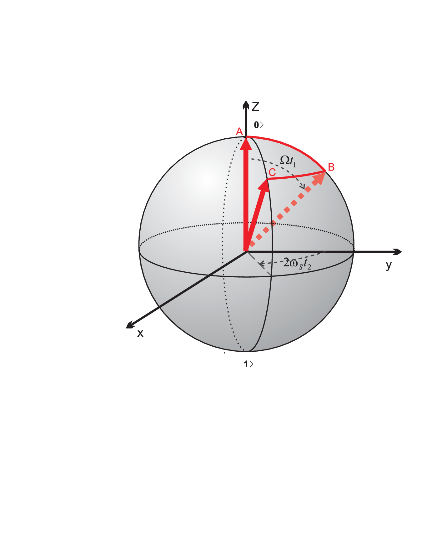
The control protocol here is illustrated in the Fig. 2. Since an arbitrary state of the two-level system can be expresses as $\left|\Phi\right\rangle_{S}=\cos\theta\left|0\right\rangle_{S}+\sin\theta e^{i\varphi}\left|1\right\rangle_{S}$, we can conclude that we can prepare the two level system to arbitrary states by choosing appropriate $t_{1}$ and $t_{2}$. This proves the controllability directly.

Before concluding our paper, we point out that there is no limit to the control scheme, and it is different from the observation in Ref. xue that there is a phase uncertainty due to the standard quantum limit. The Hamiltonian we use here is non-demolition of the accessor, while the one in Ref. xue is of the system. And it preserves the separability of the wave function. Therefore, there is no control limit to our scheme.

In this paper, we propose a general scheme to manipulate the quantum states of a quantum system by preparing the initial state of the accessor. Different from our previous approach ind3, we control the controlled system by preparing the state of the accessor. Based on the scheme, we simplify the model and point out its equivalence to broadly investigated direct quantum control. And we take advantage of the proof of controllability of direct quantum control and prove the controllability of arbitrary finite dimensional quantum system. We investigated the concrete control process of our indirect control scheme with two-level system as an example. It is found that the two-level system to reach any given target state by preparing the initial state of accessor (a qubit)only one time and the time evolution supplies the relative phase of the target state.

Finally, we point out that it is very important to study the concrete control protocol of our scheme for arbitrary finite dimensional quantum systems proposed in this paper. Generalization of our approach to infinite dimensional quantum systems will be also in consideration.

This work is supported by the NSFC with grant No.190203018, 10474104 and 60433050, 0675085, and NFRPC with No. 2001CB309310 and 2005CB724508.

References

- (1) G. M. Huang, T. J. Tarn and J. W. Clark, J. Math. Phys. 24, 2608 (1983).
- (2) Information Complexity and Control in Quantum Physics, edited by A. Blaquiere, S. Dinerand and G. Lochak (Springer, New York, 1987).
- (3) A. G. Butkovskiy and Yu. I. Samoilenko, Control of Quantum-mechanical Processes and Systems (Kluwer Academic, Dordrecht, 1990).
- (4) V. Jurdjevic, Geometric Control Theory, Cambridge University Press, 1997.
- (5) W. S. Warren, H. Rabitz, and M. Dahleh, Science 259, 1581 (1993).
- (6) V. Ramakrishna and H. Rabitz, Phys. Rev. A 54, 1715 (1996).
- (7) L. Viola, E. Knill, and S. Lloyd, Phys. Rev. Lett. 82, 2417 (1999);
- (8) S. Lloyd, Phys. Rev. A 62, 022108 (2000).
- (9) H. Rabitz et al., Science 288, 824 (2000).
- (10) L. Roa, A. Delgado, M. L. Ladronde-Guevara, and A. B. Klimov, Phys. Rev. A 73, 012322 (2006)
- (11) N. Ganesan and T. J. Tarn, Phys. Rev. A 75, 032323 (2007).
- (12) Fei Xue, S.X. Yu, C.P. Sun Phys. Rev. A 73, 013403 (2006).
- (13) H. C. Fu, Hui Dong, X. F. Liu and C.P. Sun, Phys. Rev. A 75, 052317 (2007).
- (14) R. Romano and D. D’Alessandro, Phys. Rev. A 73, 022323 (2006).
- (15) R. Romano and D. D’Alessandro, Phys. Rev. Lett. 97, 080402 (2006).
- (16) R. Romano, arXiv:0709.1675; R. Romano, arXiv:0707.3383.
- (17) H. Fu, S. G. Schirmer and A. I. Solomon, J. Phys. A. 34, 1679 (2001).
- (18) S. G. Schirmer, H. Fu and A. I. Solomon, Phys. Rev. A. 63, 063410 (2001).
- (19) R.-B. Wu, T.-J. Tarn, and C.-W. Li, Phys. Rev. A 73, 012719 (2006).
- (20) V. Jurdjevic and H. J. Sussmann, J. Diff. Eq. 12, 313 (1972).