跳到论文正文
W Papers独立论文阅读器 arXiv:0712.0396 论文正文 计算阅读时间 · 0%
引用这篇论文根据当前论文元数据生成,正式投稿前建议核对。


License: Assumed arXiv.org perpetual non-exclusive license
arXiv:0712.0396v1 [hep-ph] 03 Dec 2007

Electroweak Corrections in High Energy Processes using Effective Field Theory

Jui-yu Chiu Affiliation: Department of Physics, University of California at San Diego, La Jolla, CA 92093    Frank Golf Affiliation: Department of Physics, University of California at San Diego, La Jolla, CA 92093    Randall Kelley Affiliation: Department of Physics, University of California at San Diego, La Jolla, CA 92093    Aneesh V. Manohar Affiliation: Department of Physics, University of California at San Diego, La Jolla, CA 92093
August 11, 2026 18:33
Abstract

Electroweak Sudakov logarithms at high energy, of the form (α/sin2⁡θW)n​logm​s/MZ,W2(\alpha/\sin^{2}\theta_{W})^{n}\log^{m}s/M_{Z,W}^{2}, are summed using effective theory methods. The corrections are computed to processes involving two external particles in the standard model. The results include non-zero particle masses, such as the tt-quark mass, electroweak mixing effects which lead to unequal WW and ZZ masses, and radiative Higgs corrections proportional to the Yukawa couplings. We show that the matching at the scale MW,ZM_{W,Z} has a term at most linear in log⁡s/μ2\log s/\mu^{2} to all orders. The effective theory formalism is compared with, and extends, previous work based on infrared evolution equations.

I Introduction

The Large Hadron Collider (LHC) has a center-of-mass energy of s=14\sqrt{s}=14 TeV, and will be able to measure collisions with a partonic center-of-mass energy of several TeV, more than an order of magnitude larger than the masses of the electroweak gauge bosons. Radiative corrections to scattering processes depend on the ratio of mass scales, and radiative corrections at high energy depend on logarithms of the form log⁡s/MW,Z2\log s/M^{2}_{W,Z}. In high energy exclusive processes, radiative corrections are enhanced by two powers of a large logarithm for each order in perturbation theory, and the logarithms are often referred to as Sudakov (double) logarithms. Electroweak Sudakov corrections are not small at LHC energies, since α​log2​s/MW,Z2/(4​π​sin2⁡θW)∼0.15\alpha\log^{2}s/M^{2}_{W,Z}/(4\pi\sin^{2}\theta_{W})\sim 0.15 at s=4\sqrt{s}=4 TeV. These Sudakov corrections lead to a breakdown of fixed order perturbation theory, and need to be summed to all orders.

Electroweak corrections at high energy have double logarithms, even for processes which are conventionally called inclusive, such as the total e+​e−e^{+}e^{-} cross-section at large angles, because the colliding particles are not electroweak gauge singlets ccc. There are no electroweak singlet fields in the standard model. A composite particle such as the proton, while a color singlet, is not an electroweak singlet.

There is an extensive literature on electroweak Sudakov effects ciafaloni; fadin; kps; fkps; jkps; jkps4; beccaria; dp1; dp2; hori; beenakker; dmp; pozzorini; js. The computations use infrared evolution equations fadin, based on an analysis of the infrared structure of the perturbation theory amplitude and a factorization theorem for the Sudakov form factor pqcd. These summations have been checked against one-loop beccaria; dp1; dp2 and two-loop hori; beenakker; dmp; pozzorini; js computations.

The Sudakov logarithm log⁡(s/MW,Z2)\log(s/M_{W,Z}^{2}) can be thought of as an infrared logarithm in the electroweak theory, since it diverges as MW,Z→0M_{W,Z}\to 0. By using an effective field theory (EFT), these infrared logarithms in the original theory can be converted to ultraviolet logarithms in the effective theory, and summed using standard renormalization group techniques. The effective theory needed is soft-collinear effective theory (SCET) BFL; SCET, which has been used to study high energy processes in QCD, and to perform Sudakov resummations arising from radiative gluon corrections.

This paper studies high energy electroweak Sudakov corrections using SCET, and expands on our previous work cgkm1. In Ref. cgkm1, we showed how to compute log⁡s/MW,Z2\log s/M^{2}_{W,Z} corrections to the Sudakov form factor for massless fermions using EFT methods. In this paper, the results are generalized to massive fermions such as the top quark, and include radiative corrections due to Higgs exchange. The corrections are computed without assuming that the Higgs and electroweak gauge bosons are degenerate in mass, as in previous calculations. A new feature of EFT matching, the existence of single logarithmic matching corrections cgkm1, is discussed in detail, and proven to be true to all orders in perturbation theory. This paper discusses the Sudakov form factor computation in detail. The Sudakov form factor is not of direct relevance to LHC processes, but it allows us to illustrate the EFT method for operators involving two external particles. The computations of the Sudakov form factor given in this paper can be used to compute electroweak corrections to processes relevant for the LHC, such as dijet production, t​t¯t\bar{t} production, or squark pair production, which involve operators with four external particles. The results are given in a future publication cgkm3, and can be obtained from the computations given in this paper by summing over all pairs of external particles with the appropriate group theoretic factors.

The outline of the calculation is given in Sec. II. The SCET formalism and the full theory we use for our calculations are described in Sec. III. Known results on the exponentiation of the Sudakov form factor, and a comparison of the infrared evolution equation formalism with the SCET approach is given in Sec. IV. Section V discusses the calculation of Sudakov corrections for massive gauge bosons and massless external particles. Section VI gives the proof that there is at most a single logarithm found in the matching condition to all orders in perturbation theory, and consistency conditions on the matching coefficients and anomalous dimensions are given in Sec. VII. The extension to massive external particles is given in Sec. VIII for all possible hierarchies of mass-scales, including cases in which particle masses are not widely separated, so that multiple scales have to be integrated out simultaneously. Massive scalar exchange graphs, relevant for Higgs exchange, are computed in Sec. IX. Applications of the formalism to electroweak Sudakov corrections in the standard model is given in Sec. X for light quarks, the top quark, and leptons.

Notation: We use a⁡(μ)≡α⁡(μ)/(4​π)a(\mu)\equiv\alpha(\mu)/(4\pi), and ai​(μ)≡αi​(μ)/(4​π)a_{i}(\mu)\equiv\alpha_{i}(\mu)/(4\pi) where i=s,2,1i=s,2,1 for the QCD, S​U​(2)SU(2) and U⁡(1)U(1) couplings in the standard model. Hypercharge is normalized so that Q=T3+YQ=T_{3}+Y. Logarithms are denoted by 𝖫A≡log⁡A2/μ2\mathsf{L}_{A}\equiv\log A^{2}/\mu^{2}, for A=Q,M,m1,m2A=Q,M,m_{1},m_{2}. CFC_{F} and TFT_{F} are the Casimir and index for the external particles. We use the subscript FF for both fermions and scalars, to avoid rewriting the same expression twice.

II Outline of Calculation

The physical quantity we study is the Sudakov form factor in the Euclidean region, defined as the amplitude FE​(Q2)=⟨p2|𝒪|p1⟩F_{E}(Q^{2})=\braket{p_{2}|\mathcal{O}|p_{1}} for the scattering of on-shell particles pi2=mi2p_{i}^{2}=m_{i}^{2} by an operator 𝒪\mathcal{O}, with Q2=−(p2−p1)2>0Q^{2}=-(p_{2}-p_{1})^{2}>0. The timelike Sudakov form factor is given by analytic continuation, F⁡(s)=FE​(−s−i​0+)F(s)=F_{E}(-s-i0^{+}), so that log⁡(Q2/μ2)→log⁡(s/μ2)−i​π\log(Q^{2}/\mu^{2})\to\log(s/\mu^{2})-i\pi.

We will compute FE​(Q2)F_{E}(Q^{2}) for fermion scattering by 𝒪=ψ¯​γμ​ψ,ψ¯​ψ,ψ¯​σμ​ν​ψ\mathcal{O}=\bar{\psi}\gamma^{\mu}\psi,\,\bar{\psi}\psi,\,\bar{\psi}\sigma^{\mu\nu}\psi, scalars scattering by 𝒪=ϕ†​ϕ,i⁡(ϕ†​Dμ​ϕ−Dμ​ϕ†​ϕ)\mathcal{O}=\phi^{\dagger}\phi,\,i(\phi^{\dagger}D^{\mu}\phi-D^{\mu}\phi^{\dagger}\phi), and fermion to scalar (or vice-versa) scattering by 𝒪=ψ¯​ϕ\mathcal{O}=\bar{\psi}\phi. All operators are taken to be gauge singlets so the incoming and outgoing particles have the same gauge quantum numbers, but not necessarily the same mass.

The form factor, FE​(Q2)F_{E}(Q^{2}) is computed using a sequence of effective theories. For the high energy process considered is this paper, there are several widely separated scales and we must switch to the relevant theory as we move between scales. At scales higher than Q2Q^{2}, the theory is the original gauge theory, referred to as the full theory in EFT terminology. The precise theory, and the SCET formalism used are given in Sec. III.

As we move to scales below Q2Q^{2} we transition to an effective field theory (SCET) where degrees of freedom with offshellness on the order of Q2Q^{2} are integrated out. The full and EFT have the same infrared (IR) physics but different ultraviolet (UV) behavior and to ensure that the operators in the respective theories have the same on-shell matrix elements, we must introduce a matching coefficient, exp⁡[C⁡(μ)]\exp[C(\mu)]. For later convenience, the matching coefficient is written as an exponential. If the full theory is matched onto SCET at μQ\mu_{Q} then the matching coefficient is chosen so that

⟨p2|𝒪⁡(μQ)|p1⟩\displaystyle\braket{p_{2}|\mathcal{O}(\mu_{Q})|p_{1}} =\displaystyle= exp⁡[C⁡(μQ)]​⟨p2|𝒪~​(μQ)|p1⟩\displaystyle\exp[C(\mu_{Q})]\braket{p_{2}|\widetilde{\mathcal{O}}(\mu_{Q})|p_{1}} (1)

where 𝒪~​(μ)\tilde{\mathcal{O}}(\mu) is the EFT operator corresponding to the full theory operator 𝒪⁡(μ)\mathcal{O}(\mu). The matching coefficient exp⁡C⁡(μQ)\exp C(\mu_{Q}) is independent of infrared physics, and can be computed if perturbation theory is valid at μQ\mu_{Q}. In general, a single operator 𝒪\mathcal{O} can match onto a set of operators 𝒪~i\widetilde{\mathcal{O}}_{i} in the EFT with the same quantum numbers. This occurs, for example, for four-fermion operators in the analysis of high-energy parton scattering, and can be included by treating all the equations below as matrix equations, as is familiar from the well-known analysis of operator mixing. The matching coefficient C⁡(μQ)C(\mu_{Q}) contains log⁡μQ2/Q2\log\mu_{Q}^{2}/Q^{2} terms, and there are no large logarithms if μQ\mu_{Q} is chosen to be of order QQ. We will choose μQ=Q\mu_{Q}=Q, though any value of order QQ is acceptable. Any physical observable is independent of the choice for μQ\mu_{Q}. It is conventional to choose c⁡(μ)c(\mu), the coefficient of 𝒪\mathcal{O} in the full theory, to equal unity at μ=Q\mu=Q. With this choice, which gives the usual normalization for FE​(Q2)F_{E}(Q^{2}), c⁡(Q)=exp⁡C⁡(Q)c(Q)=\exp C(Q) is the coefficient of 𝒪~\widetilde{\mathcal{O}} in SCET at μ=Q\mu=Q. The evolution of c⁡(μ)c(\mu) between scales is given by the renormalization group equation

μ​d​c​(μ)d​μ=γ⁡(μ)​c​(μ),\mu\frac{dc(\mu)}{d\mu}=\gamma(\mu)c(\mu), (2)

where γ⁡(μ)\gamma(\mu) is the anomalous dimension of 𝒪~\widetilde{\mathcal{O}} in the EFT.

We must repeat this sequence of matching and renormalization group evolution as various energy scales are crossed, and more and more degrees of freedom are integrated out. An advantage of the EFT approach is that it divides the full multiscale computation into several simpler pieces, each of which depends on a single scale. This allows one to easily identify which quantities are universal, and which ones depend on the specific process. In an EFT calculation, the IR divergences in the theory above a matching scale must match with the UV divergences in the theory below the matching scale. We have checked this explicitly for all the computations in this paper. In most of the tables, we have given only the finite parts of the graphs.

III SCET Formalism

SCET is an effective theory that describes energetic particles, with energy of order QQ, where QQ is some large scale which characterizes the scattering process. SCET contains all the modes of the full theory with invariant mass much smaller than Q2Q^{2}. The SCET fields and Lagrangian depend on two null four-vectors nn and n¯\bar{n}, with n=(1,𝐧)n=(1,\bf{n}) and n¯=(1,−𝐧)\bar{n}=(1,-\bf{n}), where 𝐧\bf{n} is a unit vector, so that n¯⋅n=2\bar{n}\cdot n=2. In the Sudakov problem, one works in the Breit frame, with nn chosen to be along the p2p_{2} direction, so that n¯\bar{n} is along the p1p_{1} direction. The momentum transfer qq has no time component, q0=0q^{0}=0, so that the particle is back-scattered. The light-cone components of a four-vector pp are defined by p+≡n⋅pp^{+}\equiv n\cdot p, p−≡n¯⋅pp^{-}\equiv\bar{n}\cdot p. In our problem, p1−=p1⟂=p2+=p2⟂=0p_{1}^{-}=p_{1\perp}=p_{2}^{+}=p_{2\perp}=0, and Q2=p1+​p2−Q^{2}=p_{1}^{+}p_{2}^{-}. A fermion moving in a direction close to nn is described by the nn-collinear SCET field ξn,p​(x)\xi_{n,p}(x), where pp is a label momentum, and has components n¯⋅p\bar{n}\cdot p and p⟂p_{\perp} BFL; SCET. It describes particles (on- or off-shell) with energy 2​E=n¯⋅p2E=\bar{n}\cdot p, and p2≪Q2p^{2}\ll Q^{2}. The SCET power counting is p−∼Qp^{-}\sim Q, p+∼Q​λ2p^{+}\sim Q\lambda^{2}, p⟂∼Q​λp_{\perp}\sim Q\lambda, where λ≪1\lambda\ll 1 is the power counting parameter used for the EFT expansion. The total momentum of the field ξn,p​(x)\xi_{n,p}(x) is p+kp+k, where kk is the residual momentum of order Q​λ2Q\lambda^{2} contained in the Fourier transform of xx. Note that the label momentum pp only contributes to the minus and ⟂\perp components of the total momentum.

The gauge field is represented by several distinct fields in the effective theory: nn-collinear fields An,p​(x)A_{n,p}(x) and n¯\bar{n}-collinear fields An¯,p​(x)A_{\bar{n},p}(x) with labels, and ultrasoft fields A⁡(x)A(x) with no label, analogous to the soft and ultrasoft fields introduced in NRQCD lmr. The nn-collinear field contains gluons with momentum near the nn-direction, and momentum scaling n¯⋅p∼Q\bar{n}\cdot p\sim Q, n⋅p∼Q​λ2n\cdot p\sim Q\lambda^{2}, p⟂∼Q​λp_{\perp}\sim Q\lambda, and the n¯\bar{n}-collinear fields contain gluons moving near the n¯\bar{n}-direction, with momentum scaling n⋅p∼Qn\cdot p\sim Q, n¯⋅p∼Q​λ2\bar{n}\cdot p\sim Q\lambda^{2}, p⟂∼Q​λp_{\perp}\sim Q\lambda. The ultrasoft field contains gluons with all momentum components scaling as Q​λ2Q\lambda^{2}.

The EFT fermion field satisfies the constraint

n̸​n¯4​ξn,p\displaystyle\frac{\not{n}\not{\bar{n}}}{4}\xi_{n,p} =\displaystyle= ξn,p,\displaystyle\xi_{n,p}, (3)

where

Pn=n̸​n¯4,Pn¯=n¯​n̸4,Pn+Pn¯=1,\displaystyle P_{n}=\frac{\not{n}\not{\bar{n}}}{4},\quad P_{\bar{n}}=\frac{\not{\bar{n}}\not{n}}{4},\quad P_{n}+P_{\bar{n}}=1, (4)

are projection operators. The leading order fermion Lagrangian is SCET

ξ¯n,p​n¯2​(i​n⋅D+p⟂2n¯⋅p)​ξn,p+…,\displaystyle\bar{\xi}_{n,p}\frac{\not{\bar{n}}}{2}\left(in\cdot D+\frac{p_{\perp}^{2}}{\bar{n}\cdot p}\right)\xi_{n,p}+\ldots\,, (5)

where iD=i∂+gAiD=i\partial+gA is the ultrasoft covariant derivative, and …\ldots denotes terms involving the collinear gauge field. The fermion propagator is

n̸​n¯⋅p2​p2.\displaystyle\frac{\not{n}\ \bar{n}\cdot p}{2p^{2}}. (6)

The effective theory knows about the large momentum scale QQ through the labels n¯⋅p2\bar{n}\cdot p_{2} and n⋅p1n\cdot p_{1} on the fields ξn,p2\xi_{n,p_{2}} and ξn¯,p1\xi_{\bar{n},p_{1}} for the outgoing and incoming particles. As a result, SCET anomalous dimensions can depend on QQ. However, there are no modes in SCET which couple n¯⋅p2\bar{n}\cdot p_{2} to n⋅p1n\cdot p_{1}, so that SCET does not contain modes with off-shellness of order Q2Q^{2}, which are present in the full theory.

We will also need to introduce SCET fields to describe energetic scalar particles, such as the Higgs boson. We will use Φn,p\Phi_{n,p} as the nn-collinear field for a scalar particle moving in a direction close to nn, analogous to ξn,p\xi_{n,p} for fermions. The field Φn,p\Phi_{n,p} is normalized the same way as the full-theory field ϕ\phi, and produces scalar particles with amplitude unity. The scalar kinetic energy term becomes

Dμ​ϕ†​Dμ​ϕ→Φn,p†​[(n¯⋅p)​(i​n⋅D)+p⟂2]​Φn,p\displaystyle D_{\mu}\phi^{\dagger}D^{\mu}\phi\to\Phi_{n,p}^{\dagger}\left[\left(\bar{n}\cdot p\right)\left(in\cdot D\right)+p_{\perp}^{2}\right]\Phi_{n,p} (7)

in the effective theory. It is also convenient to use a redefined scalar field,

ϕn,p=(n¯⋅p)​Φn,p,\displaystyle\phi_{n,p}=\sqrt{\left(\bar{n}\cdot p\right)}\,\Phi_{n,p}, (8)

in terms of which the kinetic term becomes

L\displaystyle L =\displaystyle= ϕn,p†​(i​n⋅D+p⟂2n¯⋅p)​ϕn,p\displaystyle\phi_{n,p}^{\dagger}\left(in\cdot D+\frac{p_{\perp}^{2}}{\bar{n}\cdot p}\right)\phi_{n,p} (9)

and has the same normalization as the fermion Lagrangian Eq. (5). The rescaled scalar propagator is now

1p2\displaystyle\frac{1}{p^{2}} →\displaystyle\to n¯⋅pp2.\displaystyle\frac{\bar{n}\cdot p}{p^{2}}. (10)

ϕn,p\phi_{n,p} produces scalar particles moving in the nn-direction with amplitude (n¯⋅p)\sqrt{\left(\bar{n}\cdot p\right)}.

The theory we consider is a S​U​(2)SU(2) spontaneously broken gauge theory, with a Higgs in the fundamental representation, where all gauge bosons have a common mass, MM. This is the theory used in many previous computations kps; fkps; jkps; jkps4; js, and allows us to compare with previous results. It is convenient, as in Ref. js, to write the group theory factors using CFC_{F}, CAC_{A}, TFT_{F} and nFn_{F}, where 2​nF2n_{F} is defined to be the number of weak doublets Weyl fermions.11 1 This convention for nFn_{F} is used in Ref. js. Note that the results only hold for CA=2C_{A}=2, since for an S​U​(N)SU(N) group with N>2N>2, a fundamental Higgs does not break the gauge symmetry completely. We will consider this theory with fermionic and scalar matter fields in arbitrary gauge representations, with the fermions assumed to be vector-like. These fields are the external particles in the operators 𝒪\mathcal{O}. We will also need to consider graphs which are analogous to Higgs exchange graphs in the standard model. For this purpose, we will add a gauge singlet scalar field χ\chi, which couples to the fermions and scalars via gauge-invariant interactions,

Lint\displaystyle L_{\text{int}} =\displaystyle= −hψ,i​χ​ψ¯i​ψi−hϕ,i​χ​ϕi†​ϕi,\displaystyle-h_{\psi,i}\chi\bar{\psi}_{i}\psi_{i}-h_{\phi,i}\chi\phi_{i}^{\dagger}\phi_{i}, (11)

hψ,ih_{\psi,i} is dimensionless, and hϕ,ih_{\phi,i} has dimensions of mass. We will assume that hϕ,ih_{\phi,i} is independent of QQ for power counting purposes. In our toy example, χ\chi is a gauge singlet field, and does not break the gauge symmetry. The fermion masses are independent of the Yukawa couplings of χ\chi. The toy example Higgs field is a doublet, and breaks the gauge symmetry, but does not couple to the matter fields. In the standard model, the Higgs field breaks the gauge symmetry, and also has Yukawa couplings which generate fermion masses.

The computations are extended to the S​U​(3)×S​U​(2)L×U​(1)YSU(3)\times SU(2)_{L}\times U(1)_{Y} standard model in Sec. X, including Higgs exchange corrections and unequal gauge boson masses. Our results are given to leading order in the EFT power counting, i.e. we neglect power corrections of the form mi2/Q2m_{i}^{2}/Q^{2}, and M2/Q2M^{2}/Q^{2}, while retaining all logarithmic corrections log⁡mi2/Q2\log m_{i}^{2}/Q^{2} and log⁡M2/Q2\log M^{2}/Q^{2}. The gauge boson exchange graphs can be obtained from those of the toy model. In the standard model, the Higgs field breaks the gauge symmetry, and also has Yukawa couplings to the chiral fermions. At one-loop, we can obtain the Higgs exchange corrections from the χ\chi-exchange graphs in our toy example. Graphs with Higgs bosons coupling to both the fermions and the gauge bosons start at two-loops (see Fig. 1).

Refer to caption
Figure 1: Graphs in the standard model involving both Yukawa and gauge couplings which have no analog in the toy example.

IV Exponentiation

We start by summarizing some known properties of the Sudakov form-factor collins for the vector current. We will see later how the same expressions can be rederived using renormalization group methods in SCET. The Euclidean form-factor FE​(Q2)F_{E}(Q^{2}) has the expansion (𝖫=log⁡(Q2/M2)\mathsf{L}=\log(Q^{2}/M^{2}))

FE\displaystyle F_{E} =\displaystyle= 1\displaystyle 1 (12)
+α⁡(k12​𝖫2+k11​𝖫+k10)\displaystyle+\alpha\left(k_{12}\mathsf{L}^{2}+k_{11}\mathsf{L}+k_{10}\right)
+α2​(k24​𝖫4+k23​𝖫3+k22​𝖫2+k21​𝖫+k20)\displaystyle+\alpha^{2}\left(k_{24}\mathsf{L}^{4}+k_{23}\mathsf{L}^{3}+k_{22}\mathsf{L}^{2}+k_{21}\mathsf{L}+k_{20}\right)
+α3​(k36​𝖫6+…)+…,\displaystyle+\alpha^{3}\left(k_{36}\mathsf{L}^{6}+\ldots\right)+\ldots\,,

with the αn\alpha^{n} term having powers of 𝖫\mathsf{L} up to 𝖫2​n\mathsf{L}^{2n}. In the literature, the highest power of 𝖫\mathsf{L} is called the LLF\text{LL}_{\text{F}} term, the next power is called the NLLF\text{NLL}_{\text{F}} term, etc. We have included the subscript FF (for the form-factor) to distinguish it from the renormalization group counting described below.

The series for log⁡FE​(Q2)\log F_{E}(Q^{2}) takes a simpler form

log⁡FE\displaystyle\log F_{E} =\displaystyle= α⁡(k~12​𝖫2+k~11​𝖫+k~10)\displaystyle\alpha\left(\tilde{k}_{12}\mathsf{L}^{2}+\tilde{k}_{11}\mathsf{L}+\tilde{k}_{10}\right) (13)
+α2​(k~23​𝖫3+k~22​𝖫2+k~21​𝖫+k~20)\displaystyle+\alpha^{2}\left(\tilde{k}_{23}\mathsf{L}^{3}+\tilde{k}_{22}\mathsf{L}^{2}+\tilde{k}_{21}\mathsf{L}+\tilde{k}_{20}\right)
+α3​(k~34​𝖫4+…)+…,\displaystyle+\alpha^{3}\left(\tilde{k}_{34}\mathsf{L}^{4}+\ldots\right)+\ldots\,,

with the αn\alpha^{n} term having powers of 𝖫\mathsf{L} up to 𝖫n+1\mathsf{L}^{n+1}, and the expansion begins at order α\alpha. Note that Eq. (13) implies non-trivial relations among the coefficients kn​mk_{nm} in Eq. (12). At order nn, there are 2​n+12n+1 coefficients kn​mk_{nm}, 0≤m≤2​n0\leq m\leq 2n in Eq. (12), but only n+2n+2 coefficients k~n​m\tilde{k}_{nm}, 0≤m≤n+10\leq m\leq n+1 in Eq. (13).

The right-hand-side (rhs) of Eq. (13) can be written in terms of the LL series 𝖫​f0​(α​𝖫)=k~12​α​𝖫2+k~23​α2​𝖫3+…\mathsf{L}f_{0}(\alpha\mathsf{L})=\tilde{k}_{12}\alpha\mathsf{L}^{2}+\tilde{k}_{23}\alpha^{2}\mathsf{L}^{3}+\ldots, the NLL series f1​(α​𝖫)=k~11​α​𝖫+k~22​α2​𝖫2+…f_{1}(\alpha\mathsf{L})=\tilde{k}_{11}\alpha\mathsf{L}+\tilde{k}_{22}\alpha^{2}\mathsf{L}^{2}+\ldots, the NNLL series α​f2​(α​𝖫)=k~10​α+k~21​α2​𝖫+…\alpha f_{2}(\alpha\mathsf{L})=\tilde{k}_{10}\alpha+\tilde{k}_{21}\alpha^{2}\mathsf{L}+\ldots etc. as

log⁡FE\displaystyle\log F_{E} =\displaystyle= 𝖫​f0​(α​𝖫)+f1​(α​𝖫)+α​f2​(α​𝖫)+….\displaystyle\mathsf{L}f_{0}(\alpha\mathsf{L})+f_{1}(\alpha\mathsf{L})+\alpha f_{2}(\alpha\mathsf{L})+\ldots\,. (14)

f0f_{0} and f1f_{1} begin at order α\alpha, and the remaining fnf_{n} begin at order one.

In this paper, LL, NLL, etc. (with no subscripts) will refer to the counting for log⁡FE\log F_{E}. This is also the counting appropriate for a renormalization group improved computation, and is different from the conventional counting discussed above. If one looks at the order α2\alpha^{2} terms, for example, the conventional counting is that the 𝖫4\mathsf{L}^{4} term is LLF\text{LL}_{\text{F}}, the 𝖫3\mathsf{L}^{3} term is NLLF\text{NLL}_{\text{F}}, the 𝖫2\mathsf{L}^{2} term is N2​LLF\text{N}^{2}\text{LL}_{\text{F}}, the 𝖫\mathsf{L} term is N3​LLF\text{N}^{3}\text{LL}_{\text{F}}, and the 𝖫0\mathsf{L}^{0} term is N4​LLF\text{N}^{4}\text{LL}_{\text{F}}. Using our counting, the terms are given by exponentiating log⁡FE\log F_{E} to LL, NLL, N2​LL\text{N}^{2}\text{LL}, N2​LL\text{N}^{2}\text{LL}, and N3​LL\text{N}^{3}\text{LL}, respectively. At higher orders, the mismatch in powers of N between the two counting methods increases.

For precision electroweak studies, the first few orders are sufficient. Typical loop corrections are suppressed by α/(4​π)\alpha/(4\pi). There can be large coefficients in the perturbation expansion. For example, there are large coefficients in the cusp anomalous dimension (see Eqs. (54,)). In this paper we have computed corrections to the Sudakov form factor; for dijet production and processes involving four-particle operators, the anomalous dimensions are at least twice as large as for the Sudakov problem. For these reasons, we use the estimate α\alpha instead of α/(4​π)\alpha/(4\pi) for the size of loop corrections. For QCD, α∼0.1\alpha\sim 0.1, and for electroweak corrections, α→αem/sin2⁡θW∼0.03\alpha\to\alpha_{\text{em}}/\sin^{2}\theta_{W}\sim 0.03. log⁡s/MZ2∼8\log s/M_{Z}^{2}\sim 8 for s∼4s\sim 4 TeV, so α​𝖫∼1\alpha\mathsf{L}\sim 1 for QCD and ∼0.2\sim 0.2 for electroweak corrections. The NLL series is of order ten percent for QCD corrections, and a few percent for electroweak corrections. The NNLL series is of order a percent for QCD, and sub-percent for electroweak corrections.

IV.1 Infrared Evolution Equations

An expression for the Sudakov form-factor in the limit M/Q≪1M/Q\ll 1 with onshell massless fermions, p22=p12=0p_{2}^{2}=p_{1}^{2}=0, obtained using the evolution equations is mueller; collins; sen; js

log⁡FE​(Q2)=log⁡F0​(a⁡(M))\displaystyle\log F_{E}(Q^{2})=\log F_{0}(a(M))
+∫M2Q2d​μ2μ2[ζ(a(μ))+ξ(a(M))+∫M2μ2d​μ′ 2μ′ 2Γ(a(μ′))]\displaystyle+\int_{M^{2}}^{Q^{2}}\frac{{\rm d}\mu^{2}}{\mu^{2}}\left[\zeta(a(\mu))+\xi(a(M))+\int_{M^{2}}^{\mu^{2}}\frac{{\rm d}\mu^{\prime\,2}}{\mu^{\prime\,2}}\Gamma(a(\mu^{\prime}))\right]
(15)

in terms of functions F0F_{0}, ζ\zeta, ξ\xi and Γ\Gamma of the coupling constant, which have the expansions

F0​(a)\displaystyle F_{0}(a) =\displaystyle= 1+F0(1)​a+F0(2)​a2+…,\displaystyle 1+F_{0}^{(1)}a+F_{0}^{(2)}a^{2}+\ldots\,,
Γ⁡(a)\displaystyle\Gamma(a) =\displaystyle= Γ(1)​a+Γ(2)​a2+…,\displaystyle\Gamma^{(1)}a+\Gamma^{(2)}a^{2}+\ldots\,,
ζ⁡(a)\displaystyle\zeta(a) =\displaystyle= ζ(1)​a+ζ(2)​a2+…,\displaystyle\zeta^{(1)}a+\zeta^{(2)}a^{2}+\ldots\,,
ξ⁡(a)\displaystyle\xi(a) =\displaystyle= ξ(1)​a+ξ(2)​a2+….\displaystyle\xi^{(1)}a+\xi^{(2)}a^{2}+\ldots\,. (16)

The superscript gives the loop-order of the Feynman graphs which contribute. Γ\Gamma is known as the cusp anomalous dimension.

The gauge coupling constant gg satisfies the renormalization group evolution equation

μ​d​gd​μ\displaystyle\mu\frac{{\rm d}g}{{\rm d}\mu} =\displaystyle= βg​(g)\displaystyle\beta_{g}(g)
=\displaystyle= −b0​g316​π2−b1​g5(16​π2)2−b2​g7(16​π2)3+…,\displaystyle-b_{0}\frac{g^{3}}{16\pi^{2}}-b_{1}\frac{g^{5}}{(16\pi^{2})^{2}}-b_{2}\frac{g^{7}}{(16\pi^{2})^{3}}+\ldots\,,

or equivalently,

μ​d​ad​μ\displaystyle\mu\frac{{\rm d}a}{{\rm d}\mu} =\displaystyle= βa​(a)\displaystyle\beta_{a}(a) (18)
=\displaystyle= −2​a​(b0​a+b1​a2+b2​a3+…).\displaystyle-2a\left(b_{0}a+b_{1}a^{2}+b_{2}a^{3}+\ldots\right)\,.

The one-loop coefficient is

b0\displaystyle b_{0} =\displaystyle= 113​CA−43​TF​nF−13​TF​ns\displaystyle\frac{11}{3}C_{A}-\frac{4}{3}T_{F}n_{F}-\frac{1}{3}T_{F}n_{s} (19)

where nsn_{s} is the number of complex scalars, and 2​nF2n_{F} is the number of fermion weak doublets, in the convention of Ref. js.

After combining Eqs. (15–18) and expanding to order a​(M)3a(M)^{3}, the form factor takes the following form:

log⁡FE​(Q2)=\displaystyle\log F_{E}(Q^{2})=
[F0(1)+(ζ(1)+ξ(1))​𝖫+12​Γ(1)​𝖫2]​a​(M)\displaystyle\ \ \left[F_{0}^{(1)}+\left(\zeta^{(1)}+\xi^{(1)}\right)\mathsf{L}+\frac{1}{2}\Gamma^{(1)}\mathsf{L}^{2}\right]a(M)
+[−12(F0(1))2+F0(2)+(ζ(2)+ξ(2))𝖫\displaystyle\ \ +\left[-\frac{1}{2}\left(F_{0}^{(1)}\right)^{2}+F_{0}^{(2)}+\left(\zeta^{(2)}+\xi^{(2)}\right)\mathsf{L}\right.
+12(Γ(2)−b0ζ(1))𝖫2−16(b0Γ(1))𝖫3]a(M)2\displaystyle\ \ +\left.\frac{1}{2}\left(\Gamma^{(2)}-b_{0}\zeta^{(1)}\right)\mathsf{L}^{2}-\frac{1}{6}\left(b_{0}\Gamma^{(1)}\right)\mathsf{L}^{3}\right]a(M)^{2}
+[13(F0(1))3−F0(1)F0(2)+F0(3)+(ζ(3)+ξ(3))𝖫\displaystyle\ \ +\left[\frac{1}{3}\left(F_{0}^{(1)}\right)^{3}-F_{0}^{(1)}F_{0}^{(2)}+F_{0}^{(3)}+\left(\zeta^{(3)}+\xi^{(3)}\right)\mathsf{L}\right.
+12​(Γ(3)−b1​ζ(1)−2​b0​ζ(2))​𝖫2+16​(−b1​Γ(1)CLOSE\displaystyle\ \ +\left.\frac{1}{2}\left(\Gamma^{(3)}-b_{1}\zeta^{(1)}-2b_{0}\zeta^{(2)}\right)\mathsf{L}^{2}+\frac{1}{6}\left(-b_{1}\Gamma^{(1)}\right.\right.
+2b0(b0ζ(1)−Γ(2)))𝖫3+112b02Γ(1)𝖫4]a(M)3\displaystyle\ \ +\left.\left.2b_{0}\left(b_{0}\zeta^{(1)}-\Gamma^{(2)}\right)\right)\mathsf{L}^{3}+\frac{1}{12}b_{0}^{2}\Gamma^{(1)}\mathsf{L}^{4}\right]a(M)^{3}
+….\displaystyle+\ldots\,. (20)

A comparison of this expansion with Eq. (14) shows that f0f_{0} is determined by Γ(1)\Gamma^{(1)} and b0b_{0}, f1f_{1} by Γ(1,2),ζ(1),ξ(1),b0,1\Gamma^{(1,2)},\zeta^{(1)},\xi^{(1)},b_{0,1}, and f2f_{2} by F0(1),Γ(1,2,3),ζ(1,2),ξ(2),b0,1,2F_{0}^{(1)},\Gamma^{(1,2,3)},\zeta^{(1,2)},\xi^{(2)},b_{0,1,2}. In general fnf_{n} is determined by ξ(n)\xi^{(n)} and terms up to F0(n−1),Γ(n+1),ζ(n),bnF_{0}^{(n-1)},\Gamma^{(n+1)},\zeta^{(n)},b_{n}.

The expression Eq. (15) is not unique. The identity

12​∫y2z2d​μ2μ2​∂G⁡(a⁡(μ))∂a⁡(μ)​βa​(a⁡(μ))\displaystyle\hskip-22.76228pt\frac{1}{2}\int_{y^{2}}^{z^{2}}\frac{{\rm d}\mu^{2}}{\mu^{2}}\frac{\partial G(a(\mu))}{\partial a(\mu)}\beta_{a}(a(\mu)) =\displaystyle= G⁡(a⁡(z))−G⁡(a⁡(y))\displaystyle G(a(z))-G(a(y)) (21)

can be used to show that Eq. (15) is invariant under the transformation

Γ⁡(a⁡(μ′))\displaystyle\Gamma(a(\mu^{\prime})) →\displaystyle\to Γ⁡(a⁡(μ′))+∂G⁡(a⁡(μ′))∂a​βa​(a⁡(μ′)),\displaystyle\Gamma(a(\mu^{\prime}))+\frac{\partial G(a(\mu^{\prime}))}{\partial a}\beta_{a}(a(\mu^{\prime}))\,,
ζ⁡(a⁡(μ))\displaystyle\zeta(a(\mu)) →\displaystyle\to ζ⁡(a⁡(μ))−2​G​(a⁡(μ)),\displaystyle\zeta(a(\mu))-2G(a(\mu))\,,
ξ⁡(a⁡(M))\displaystyle\xi(a(M)) →\displaystyle\to ξ⁡(a⁡(M))+2​G​(a⁡(M)).\displaystyle\xi(a(M))+2G(a(M))\,. (22)

As a result, Γ\Gamma, ζ\zeta and ξ\xi are not uniquely determined from FE​(Q2)F_{E}(Q^{2}) by Eq. (15).

IV.2 Renormalization Group Evolution Equations

The corresponding expression for FE​(Q2)F_{E}(Q^{2}) in the EFT formalism, as will be derived in Sec. V, is

log⁡FE​(Q2)=C⁡(a⁡(Q))+D0​(a⁡(M))\displaystyle\log F_{E}(Q^{2})=C(a(Q))+D_{0}(a(M))
+D1​(a⁡(M))​log⁡Q2M2\displaystyle\qquad+D_{1}(a(M))\log\frac{Q^{2}}{M^{2}}
−∫MQd​μμ[A(a(μ))logμ2Q2+B(a(μ))],\displaystyle-\int_{M}^{Q}\frac{{\rm d}\mu}{\mu}\left[A(a(\mu))\log\frac{\mu^{2}}{Q^{2}}+B(a(\mu))\right]\,, (23)

where exp⁡C⁡(a⁡(Q))\exp C(a(Q)) is the multiplicative matching coefficient at Q2Q^{2}, γ⁡(μ)=A⁡(a⁡(μ))​log⁡(μ2/Q2)+B⁡(a⁡(μ))\gamma(\mu)=A(a(\mu))\log(\mu^{2}/Q^{2})+B(a(\mu)) is the SCET anomalous dimension between QQ and MM, and exp⁡D⁡(a⁡(M))\exp D(a(M)), D⁡(a⁡(M))=D0​(a⁡(M))+D1​(a⁡(M))​log​Q2/M2D(a(M))=D_{0}(a(M))+D_{1}(a(M))\log{Q^{2}}/{M^{2}} is the multiplicative matching coefficient at MM. The matching coefficient CC and the SCET anomalous dimension γ\gamma are independent of physics at the low scale MM, and so do not depend on the gauge boson and Higgs masses. The new feature of the massive gauge boson calculation is the existence of a single-log term, D1​(a​(M))D_{1}(a(M)) in the matching at MM. That there are no higher powers of log⁡Q2/M2\log Q^{2}/M^{2} in the matching is proved to hold to all orders in Sec. VI. A,B,C,D0,1A,B,C,D_{0,1} have loop expansions analogous to Eq. (16). The Nn​LL\text{N}^{n}\text{LL} series for log⁡FE\log F_{E} requires A(n+1)A^{(n+1)}, B(n)B^{(n)}, D(n)D^{(n)}, and C(n−1)C^{(n-1)}. D(n)D^{(n)} contributes only to the αn​𝖫\alpha^{n}\mathsf{L} term in fnf_{n}.

The identity Eq. (21) and

∫M2Q2d​μ2μ2​∫M2μ2d​μ′ 2μ′ 2​Γ​(a⁡(μ′))\displaystyle\int_{M^{2}}^{Q^{2}}\frac{{\rm d}\mu^{2}}{\mu^{2}}\int_{M^{2}}^{\mu^{2}}\frac{{\rm d}\mu^{\prime\,2}}{\mu^{\prime\,2}}\Gamma(a(\mu^{\prime})) =\displaystyle= ∫M2Q2d​μ2μ2​Γ​(a⁡(μ))​log⁡Q2μ2\displaystyle\int_{M^{2}}^{Q^{2}}\frac{{\rm d}\mu^{2}}{\mu^{2}}\Gamma(a(\mu))\log\frac{Q^{2}}{\mu^{2}}

can be used to show that Eq. (23) is unchanged by the redefinitions

A⁡(a⁡(μ))\displaystyle A(a(\mu)) →\displaystyle\to A⁡(a⁡(μ))+∂G~​(a​(μ))∂a​βa​(a⁡(μ)),\displaystyle A(a(\mu))+\frac{\partial\tilde{G}(a(\mu))}{\partial a}\beta_{a}(a(\mu))\,,
B⁡(a⁡(μ))\displaystyle B(a(\mu)) →\displaystyle\to B⁡(a⁡(μ))+∂H~​(a​(μ))∂a​βa​(a⁡(μ))\displaystyle B(a(\mu))+\frac{\partial\tilde{H}(a(\mu))}{\partial a}\beta_{a}(a(\mu))
+2​G~​(a⁡(μ)),\displaystyle+2\tilde{G}(a(\mu))\,,
C⁡(a⁡(Q))\displaystyle C(a(Q)) →\displaystyle\to C​(a​(Q))+H~​(a​(Q)),\displaystyle C(a(Q))+\tilde{H}(a(Q))\,,
D0​(a​(M))\displaystyle D_{0}(a(M)) →\displaystyle\to D0​(a⁡(M))−H~​(a⁡(M)),\displaystyle D_{0}(a(M))-\tilde{H}(a(M))\,,
D1​(a​(M))\displaystyle D_{1}(a(M)) →\displaystyle\to D1​(a⁡(M))+G~​(a⁡(M)).\displaystyle D_{1}(a(M))+\tilde{G}(a(M))\,. (25)

Transformations such as these can arise from a change of scheme in the computation of the SCET matching coefficients and anomalous dimensions.

We can now demonstrate the equivalence of the Sudakov form-factor in Eq. (23) and the form-factor given in Eq. (15). By taking G(a)=−ξ(a)/2G(a)=-\xi(a)/2 in Eq. (22), H~​(a)=−C​(a)\tilde{H}(a)=-C(a) and G~​(a)=−D1​(a)\tilde{G}(a)=-D_{1}(a) in Eq. (25), brings Eq. (15) with Eq. (23) to a common form, and gives the identifications:

12​A​(a⁡(μ))−12​∂D1​(a​(μ))∂a​βa​(a⁡(μ))\displaystyle\frac{1}{2}A(a(\mu))-\frac{1}{2}\frac{\partial D_{1}(a(\mu))}{\partial a}\beta_{a}(a(\mu))
=Γ⁡(a⁡(μ))−12​∂ξ⁡(a⁡(μ))∂a​βa​(a⁡(μ)),\displaystyle\qquad\qquad=\Gamma(a(\mu))-\frac{1}{2}\frac{\partial\xi(a(\mu))}{\partial a}\beta_{a}(a(\mu))\,,
−12​B​(a⁡(μ))+12​∂C⁡(a⁡(μ))∂a​βa​(a⁡(μ))+D1​(a⁡(μ)CLOSE\displaystyle-\frac{1}{2}B(a(\mu))+\frac{1}{2}\frac{\partial C(a(\mu))}{\partial a}\beta_{a}(a(\mu))+D_{1}(a(\mu)
=ζ⁡(a⁡(μ))+ξ⁡(a⁡(μ)),\displaystyle\qquad\qquad=\zeta(a(\mu))+\xi(a(\mu))\,,
C⁡(a⁡(M))+D0​(a⁡(M))=log⁡F0​(a⁡(M)).\displaystyle C(a(M))+D_{0}(a(M))=\log F_{0}(a(M)). (26)

The lhs of Eq. (26) is invariant under Eq. (25), and the rhs under Eq. (22). The computations of the SCET anomalous dimension and the cusp anomalous dimension in the literature use the same scheme, so that Γ=A/2\Gamma=A/2, and

12​A​(a)\displaystyle\frac{1}{2}A(a) =\displaystyle= Γ⁡(a),\displaystyle\Gamma(a)\,,
D1​(a)\displaystyle D_{1}(a) =\displaystyle= ξ⁡(a),\displaystyle\xi(a)\,,
−12​B​(a)+12​∂C⁡(a)∂a​βa​(a)\displaystyle-\frac{1}{2}B(a)+\frac{1}{2}\frac{\partial C(a)}{\partial a}\beta_{a}(a) =\displaystyle= ζ⁡(a),\displaystyle\zeta(a)\,,
C​(a)+D0​(a)\displaystyle C(a)+D_{0}(a) =\displaystyle= log⁡F0​(a).\displaystyle\log F_{0}(a)\,. (27)

The expansion of log⁡FE​(Q2)\log F_{E}(Q^{2}) to order a​(M)3a(M)^{3} using the SCET form is:

log⁡FE​(Q2)=\displaystyle\log F_{E}(Q^{2})=
[C(1)+D0(1)+(−12​B(1)+D1(1))​𝖫+14​A(1)​𝖫2]​a​(M)\displaystyle\ \ \left[C^{(1)}+D_{0}^{(1)}+\left(-\frac{1}{2}B^{(1)}+D_{1}^{(1)}\right)\mathsf{L}+\frac{1}{4}A^{(1)}\mathsf{L}^{2}\right]a(M)
+[C(2)+D0(2)+(−12B(2)−b0C(1)+D1(2))𝖫\displaystyle\ \ +\left[C^{(2)}+D_{0}^{(2)}+\left(-\frac{1}{2}B^{(2)}-b_{0}C^{(1)}+D_{1}^{(2)}\right)\mathsf{L}\right.
+14(A(2)+b0B(1))𝖫2−112(b0A(1))𝖫3]a(M)2\displaystyle\ \ +\left.\frac{1}{4}\left(A^{(2)}+b_{0}B^{(1)}\right)\mathsf{L}^{2}-\frac{1}{12}\left(b_{0}A^{(1)}\right)\mathsf{L}^{3}\right]a(M)^{2}
+[C(3)+D0(3)+(−12B(3)−b1C(1)−2b0C(2)\displaystyle\ \ +\left[C^{(3)}+D_{0}^{(3)}+\left(-\frac{1}{2}B^{(3)}-b_{1}C^{(1)}-2b_{0}C^{(2)}\right.\right.
OPEN+D1(3))​𝖫+14​(A(3)+b1​B(1)CLOSE\displaystyle\ \ \left.\left.+D_{1}^{(3)}\right)\mathsf{L}+\frac{1}{4}\left(A^{(3)}+b_{1}B^{(1)}\right.\right.
OPEN+2​b0​(B(2)+2​b0​C(1)))​𝖫2−112​(b1​A(1)CLOSE\displaystyle\left.+2b_{0}\left(B^{(2)}+2b_{0}C^{(1)}\right)\right)\mathsf{L}^{2}-\frac{1}{12}\left(b_{1}A^{(1)}\right.
+2b02B(1)+2b0A(2))𝖫3+124b02A(1)𝖫4]a(M)3.\displaystyle\ \ \left.\left.+2b_{0}^{2}B^{(1)}+2b_{0}A^{(2)}\right)\mathsf{L}^{3}+\frac{1}{24}b_{0}^{2}A^{(1)}\mathsf{L}^{4}\right]a(M)^{3}\,. (28)

V Massless External Particles

In this section we calculate the form-factor log⁡FE​(Q2)\log F_{E}(Q^{2}) for the case Q2≫M2≫m12,m22Q^{2}\gg M^{2}\gg m_{1}^{2},m_{2}^{2}. At scales μ>Q\mu>Q we use the full theory, and the renormalization group evolution of c⁡(μ)c(\mu) is given by

μ​d​c​(μ)d​μ\displaystyle\mu\frac{{\rm d}c(\mu)}{{\rm d}\mu} =\displaystyle= γF​(a​(μ))​c​(μ),\displaystyle\gamma_{F}(a(\mu))\ c(\mu)\,, (29)

where γF​(a)=γF(1)​a+γF(2)​a2+…\gamma_{F}(a)=\gamma_{F}^{(1)}a+\gamma_{F}^{(2)}a^{2}+\ldots is the full theory anomalous dimension for 𝒪\mathcal{O}. The one-loop values γF(1)\gamma_{F}^{(1)} are given in Table 1. The general form for FEF_{E} given in Sec. IV is for the vector current, where γF=0\gamma_{F}=0, and c⁡(μ>Q)c(\mu>Q) is chosen to be unity. It also holds for the other operators with c⁡(μ=Q)=1c(\mu=Q)=1 in the full theory.

𝒪γF(1)/CFC(1)​(μ)/CFγ1(1)​(μ)/CFD(1)​(μ)/CFψ¯​ψ−6−𝖫Q2+π26−24​𝖫Q−6−𝖫M2+2​𝖫M​𝖫Q−3​𝖫M+92−5​π26ψ¯​γμ​ψ0−𝖫Q2+3​𝖫Q+π26−84​𝖫Q−6−𝖫M2+2​𝖫M​𝖫Q−3​𝖫M+92−5​π26ψ¯​σμ​ν​ψ2−𝖫Q2+4​𝖫Q+π26−84​𝖫Q−6−𝖫M2+2​𝖫M​𝖫Q−3​𝖫M+92−5​π26ϕ†​ϕ−6−𝖫Q2+𝖫Q+π26−24​𝖫Q−8−𝖫M2+2​𝖫M​𝖫Q−4​𝖫M+72−5​π26i⁡(ϕ†​Dμ​ϕ−Dμ​ϕ†​ϕ)0−𝖫Q2+4​𝖫Q+π26−84​𝖫Q−8−𝖫M2+2​𝖫M​𝖫Q−4​𝖫M+72−5​π26ψ¯​ϕ,ϕ†​ψ−3−𝖫Q2+2​𝖫Q+π26−44​𝖫Q−7−𝖫M2+2​𝖫M​𝖫Q−72​𝖫M+4−5​π26\displaystyle\begin{array}[]{|c|r|c|c|c|}\hline\cr\mathcal{O}&\gamma_{F}^{(1)}/C_{F}&C^{(1)}(\mu)/C_{F}&\gamma_{1}^{(1)}(\mu)/C_{F}&D^{(1)}(\mu)/C_{F}\\ \hline\cr\bar{\psi}\psi&-6&-\mathsf{L}_{Q}^{2}+\frac{\pi^{2}}{6}-2&4\mathsf{L}_{Q}-6&-\mathsf{L}_{M}^{2}+2\mathsf{L}_{M}\mathsf{L}_{Q}-3\mathsf{L}_{M}+\frac{9}{2}-\frac{5\pi^{2}}{6}\\[5.0pt] \bar{\psi}\gamma^{\mu}\psi&0&-\mathsf{L}_{Q}^{2}+3\mathsf{L}_{Q}+\frac{\pi^{2}}{6}-8&4\mathsf{L}_{Q}-6&-\mathsf{L}_{M}^{2}+2\mathsf{L}_{M}\mathsf{L}_{Q}-3\mathsf{L}_{M}+\frac{9}{2}-\frac{5\pi^{2}}{6}\\[5.0pt] \bar{\psi}\sigma^{\mu\nu}\psi&2&-\mathsf{L}_{Q}^{2}+4\mathsf{L}_{Q}+\frac{\pi^{2}}{6}-8&4\mathsf{L}_{Q}-6&-\mathsf{L}_{M}^{2}+2\mathsf{L}_{M}\mathsf{L}_{Q}-3\mathsf{L}_{M}+\frac{9}{2}-\frac{5\pi^{2}}{6}\\[5.0pt] \phi^{\dagger}\phi&-6&-\mathsf{L}_{Q}^{2}+\mathsf{L}_{Q}+\frac{\pi^{2}}{6}-2&4\mathsf{L}_{Q}-8&-\mathsf{L}_{M}^{2}+2\mathsf{L}_{M}\mathsf{L}_{Q}-4\mathsf{L}_{M}+\frac{7}{2}-\frac{5\pi^{2}}{6}\\[5.0pt] i(\phi^{\dagger}D^{\mu}\phi-D^{\mu}\phi^{\dagger}\phi)&0&-\mathsf{L}_{Q}^{2}+4\mathsf{L}_{Q}+\frac{\pi^{2}}{6}-8&4\mathsf{L}_{Q}-8&-\mathsf{L}_{M}^{2}+2\mathsf{L}_{M}\mathsf{L}_{Q}-4\mathsf{L}_{M}+\frac{7}{2}-\frac{5\pi^{2}}{6}\\[5.0pt] \bar{\psi}\phi,\phi^{\dagger}\psi&-3&-\mathsf{L}_{Q}^{2}+2\mathsf{L}_{Q}+\frac{\pi^{2}}{6}-4&4\mathsf{L}_{Q}-7&-\mathsf{L}_{M}^{2}+2\mathsf{L}_{M}\mathsf{L}_{Q}-\frac{7}{2}\mathsf{L}_{M}+4-\frac{5\pi^{2}}{6}\\[5.0pt] \hline\cr\end{array}
Table 1: One-loop corrections to the Sudakov form-factor. γF\gamma_{F} is the full theory anomalous dimension, CC is the matching coefficient at μ∼Q\mu\sim Q, γ1\gamma_{1} is the SCET anomalous dimension, and DD is the matching coefficient at μ∼M\mu\sim M. γF(1)\gamma^{(1)}_{F}, C(1)C^{(1)}, γ1(1)\gamma^{(1)}_{1} and D(1)D^{(1)} are the coefficients of a≡α/(4​π)a\equiv\alpha/(4\pi) in the one-loop corrections, and 𝖫Q≡log⁡Q2/μ2\mathsf{L}_{Q}\equiv\log Q^{2}/\mu^{2}, 𝖫M≡log⁡M2/μ2\mathsf{L}_{M}\equiv\log M^{2}/\mu^{2}.

The full theory is matched onto SCET at a scale μ\mu of order QQ. The effective theory has modes with off-shellness of order QQ integrated out, so the matching coefficient depends on log⁡Q2/μ2\log Q^{2}/\mu^{2}, and these logarithms are not large if μ∼Q\mu\sim Q.

The operator 𝒪\mathcal{O} in the full theory matches to the operator 𝒪~\widetilde{\mathcal{O}} in SCET:

ψ¯​Γ​ψ\displaystyle\bar{\psi}\Gamma\psi →\displaystyle\to exp⁡C⁡(μ)​[ξ¯n,p2​Wn]​Γ​[Wn¯†​ξn¯,p1],\displaystyle\exp C(\mu)\,[\bar{\xi}_{n,p_{2}}W_{n}]\Gamma[W^{\dagger}_{\bar{n}}\xi_{\bar{n},p_{1}}]\,,
ϕ†​ϕ\displaystyle\phi^{\dagger}\phi →\displaystyle\to exp⁡C⁡(μ)​[Φn,p2†​Wn]​[Wn¯†​Φn¯,p1],\displaystyle\exp C(\mu)\,[\Phi_{n,p_{2}}^{\dagger}W_{n}][W^{\dagger}_{\bar{n}}\Phi_{\bar{n},p_{1}}]\,,
i​ϕ†↔Dμ​ϕ\displaystyle i\phi^{\dagger}\raise 6.45831pt\hbox{$\leftrightarrow$}\mkern-16.5muD^{\mu}\phi →\displaystyle\to exp⁡C⁡(μ)​[Φn,p2†​Wn]​(i​𝒟1+i​𝒟2)μ​[Wn¯†​Φn¯,p1],\displaystyle\exp C(\mu)\,[\Phi_{n,p_{2}}^{\dagger}W_{n}](i\mathcal{D}_{1}+i\mathcal{D}_{2})^{\mu}[W^{\dagger}_{\bar{n}}\Phi_{\bar{n},p_{1}}]\,,
ψ¯​ϕ\displaystyle\bar{\psi}\phi →\displaystyle\to exp⁡C⁡(μ)​[ξ¯n,p2​Wn]​[Wn¯†​Φn¯,p1],\displaystyle\exp C(\mu)\,[\bar{\xi}_{n,p_{2}}W_{n}][W^{\dagger}_{\bar{n}}\Phi_{\bar{n},p_{1}}]\,, (31)

where i​𝒟1=𝒫+g⁡(n⋅An¯,q)​n¯2i\mathcal{D}_{1}=\mathcal{P}+g(n\cdot A_{\bar{n},q})\frac{\bar{n}}{2}, i​𝒟2=𝒫†+g⁡(n¯⋅An,−q)​n2i\mathcal{D}_{2}=\mathcal{P}^{\dagger}+g(\bar{n}\cdot A_{n,-q})\frac{n}{2} and 𝒫\mathcal{P} are the SCET label operators introduced in Bauer et al.  SCET. Collinear gauge invariance requires that, in the matching of gauge invariant operators at leading order in the power counting, the fields occur in the combination Wn†​ξn,pW_{n}^{\dagger}\xi_{n,p}, Wn†​Φn,pW_{n}^{\dagger}\Phi_{n,p}, where WnW_{n} is a Wilson line containing nn-collinear gauge fields obtained by integrating over a path in the n¯\bar{n}-direction SCET.

C⁡(μ)C(\mu) depends on the operator being matched (i.e. the CC’s in Eq. (31) have different values, and CC can depend on Γ\Gamma) and, for convenience, we have written the multiplicative matching coefficient as exp⁡C⁡(μ)\exp C(\mu) rather than C⁡(μ)C(\mu). As is well-known, the matching coefficient can be computed as the finite part of the full theory matrix element, evaluated on-shell, with all infrared scales such as the gauge boson mass set to zero (see e.g. hqet; eft; dis). The full theory graphs to be evaluated at one-loop are those in Fig. 2,

Refer to caption
Refer to caption
Figure 2: Graphs contributing to the matching condition C⁡(α⁡(Q))C(\alpha(Q)). The solid line can be either a fermion or scalar. The second graph only exists for the scalar case 𝒪=i⁡(ϕ†​Dμ​ϕ−Dμ​ϕ†​ϕ)\mathcal{O}=i(\phi^{\dagger}D^{\mu}\phi-D^{\mu}\phi^{\dagger}\phi).

and when combined with the wavefunction and tree-level graphs, give the value of the full theory matrix element ⟨p2|𝒪|p1⟩\braket{p_{2}|\mathcal{O}|p_{1}}. The graphs for the EFT vertex correction are shown in Fig. 3, and when combined with the tree-level and wavefunction graphs, give the EFT matrix element ⟨p2|𝒪~|p1⟩\braket{p_{2}|\widetilde{\mathcal{O}}|p_{1}}. The gauge boson and fermion masses are infrared scales and can be set to zero in the matching computation thus leading to scaleless integrals for the one-loop EFT and wavefunction graphs. Since these scaleless integrals are set to zero in dimensional regularization, the EFT matrix element is equal to its tree-level value. The full theory and EFT operators 𝒪\mathcal{O} and 𝒪~\widetilde{\mathcal{O}} are normalized to have the same tree-level value, so exp⁡[C⁡(μ)]=⟨p2|𝒪|p1⟩/⟨p2|𝒪|p1⟩tree\exp[C(\mu)]=\braket{p_{2}|\mathcal{O}|p_{1}}/\braket{p_{2}|\mathcal{O}|p_{1}}_{\text{tree}}, i.e. the matching condition exp⁡C\exp C is given by the on-shell full theory matrix element normalized to its tree-level value (see e.g. Ref. hqet for more details).

The computation of the SCET one loop graphs for 𝒪=ψ¯​γμ​ψ\mathcal{O}=\bar{\psi}\gamma^{\mu}\psi is identical to that for DIS dis. Particle masses, such as the gauge boson mass, are all much smaller than QQ, and only contribute M2/Q2M^{2}/Q^{2} power corrections at the scale QQ, which are being neglected. The one-loop values of C⁡(μ)C(\mu) for the other cases are computed similarly, and are given in Table 1, where C⁡(μ)=C(1)​α​(μ)/(4​π)C(\mu)=C^{(1)}\alpha(\mu)/(4\pi) defines the one-loop correction C(1)C^{(1)}. There are no large logarithms in this matching correction if the matching scale μ\mu is chosen to be of order QQ. We will choose the matching at the high scale to be at μ=Q\mu=Q, and C⁡(μ=Q)C(\mu=Q) is given by the third column in Table 1 with 𝖫Q→0\mathsf{L}_{Q}\to 0.

The renormalization group evolution of c⁡(μ)c(\mu) in the effective theory is given by the anomalous dimension of 𝒪~\widetilde{\mathcal{O}} in SCET. The anomalous dimension γ1\gamma_{1} is used to evolve c⁡(μ)c(\mu) from μ=Q\mu=Q down to the low scale μ=M\mu=M. The one-loop anomalous dimension is given by the ultraviolet counterterms for the SCET graphs in Fig. 3 (after zero-bin subtraction, see Ref zerobin).

Refer to caption
Refer to caption
Refer to caption
Figure 3: SCET graphs for the matrix element of 𝒪~\widetilde{\mathcal{O}}. The dotted lines are SCET propagators, and represent either fermions or scalars. The upper graphs are the nn-collinear and n¯\bar{n}-collinear graphs, and the lower graph is the ultrasoft graph. There are also wavefunction graphs. For i​ϕ†↔Dμ​ϕi\phi^{\dagger}\raise 6.45831pt\hbox{$\leftrightarrow$}\mkern-16.5muD^{\mu}\phi, graph (a) also has a contribution where the gauge boson field at ⊗\otimes arises from the covariant derivative.

As noted earlier, anomalous dimensions in SCET can depend on QQ. Ultraviolet divergences do not depend on the infrared properties of the theory, such as a gauge boson mass, so the anomalous dimension for 𝒪=ψ¯​γμ​ψ\mathcal{O}=\bar{\psi}\gamma^{\mu}\psi is identical to the DIS result dis. The same argument as that given in Ref. dis for deep inelastic scattering shows that γ1​(μ)\gamma_{1}(\mu) is linear in log⁡μ2/Q2\log\mu^{2}/Q^{2} to all orders dis; Bauer:2003pi, so γ\gamma is written as

γ1​(μ)\displaystyle\gamma_{1}(\mu) =\displaystyle= A⁡(α⁡(μ))​log⁡μ2Q2+B⁡(α⁡(μ)),\displaystyle A(\alpha(\mu))\log\frac{\mu^{2}}{Q^{2}}+B(\alpha(\mu))\,, (32)

which defines AA and BB. The anomalous dimension has the expansion γ1=γ1(1)​a+γ1(2)​a2+…\gamma_{1}=\gamma^{(1)}_{1}a+\gamma^{(2)}_{1}a^{2}+\ldots, A=A(1)​a+A(2)​a2+…A=A^{(1)}a+A^{(2)}a^{2}+\ldots, B=B(1)​a+B(2)​a2+…B=B^{(1)}a+B^{(2)}a^{2}+\ldots The computations for the other cases are similar, and the results are given in Table 1. Note that the anomalous dimension depends only on the external fields for the operators, and is equal for the three fermion operators, and for the two scalar operators. The reason is that the EFT anomalous dimension depends on the IR divergence of the full theory graph, and the IR divergence is independent of the vertex factors. The anomalous dimension for ψ¯​ϕ\bar{\psi}\phi is the average of the anomalous dimensions for the fermionic and scalar operators.

The next step in the EFT computation is the matching condition at the low scale μ∼M\mu\sim M. At this scale, the massive gauge boson is integrated out, and one matches to an effective theory which is SCET without the massive gauge boson. In our toy example, this effective theory contains no gauge particles, and is a free theory. There is no need to introduce any propagating gauge modes below MM ir. The matching at μ∼M\mu\sim M is given by evaluating the graphs in Fig. 3, and the wavefunction graphs. The gauge boson mass can no longer be set to zero, since it is of the same order as the matching scale, and the one loop SCET graphs are non-zero. The matching computation is discussed in detail here for the fermion vector current. The other cases are treated similarly.

One matches the operator c⁡(μ)​[ξ¯n,p2​Wn]​γμ​[Wn¯†​ξn¯,p1]c(\mu)[\bar{\xi}_{n,p_{2}}W_{n}]\gamma^{\mu}[W^{\dagger}_{\bar{n}}\xi_{\bar{n},p_{1}}] in SCET with gauge particles (the theory above MM) onto the operator [exp⁡D⁡(μ)]​c​(μ)​ξ¯n,p2​γμ​ξn¯,p1\left[\exp D(\mu)\right]c(\mu)\bar{\xi}_{n,p_{2}}\gamma^{\mu}\xi_{\bar{n},p_{1}} in SCET without gauge particles (the theory below MM). The nn-collinear graph in Fig. 3 gives

In\displaystyle I_{n} =\displaystyle= −ig2μ2​ϵCFc(μ)∫dd​k(2​π)d1k2−M2\displaystyle-ig^{2}\mu^{2\epsilon}C_{F}c(\mu)\int{{\rm d}^{d}k\over(2\pi)^{d}}\frac{1}{k^{2}-M^{2}}
×\displaystyle\times n¯2​nα​n̸2​n¯⋅(p2−k)(p2−k)2​γμ​1−n¯⋅k​n¯α\displaystyle{\not{\bar{n}}\ \over 2}n^{\alpha}\frac{\not{n}}{2}\frac{\bar{n}\cdot(p_{2}-k)}{(p_{2}-k)^{2}}\gamma^{\mu}\frac{1}{-\bar{n}\cdot k}\bar{n}_{\alpha}
=\displaystyle= −2ig2CFγμμ2​ϵ∫dd​k(2​π)d\displaystyle-2ig^{2}C_{F}\gamma^{\mu}\mu^{2\epsilon}\int{{\rm d}^{d}k\over(2\pi)^{d}}
×\displaystyle\times n¯⋅(p2−k)[(p2−k)2+i0+][−n¯⋅k+i0+][k2−M2+i0+].\displaystyle\frac{\bar{n}\cdot(p_{2}-k)}{[(p_{2}-k)^{2}+i0^{+}][-\bar{n}\cdot k+i0^{+}][k^{2}-M^{2}+i0^{+}]}.

This integral is divergent, even in 4−2​ϵ4-2\epsilon dimensions with an off-shellness, unlike the previously studied examples where the gauge boson was massless. A related divergence was encountered by Beneke and Feldman in their study of the B→π​ℓ​νB\to\pi\ell\nu form-factor. Beneke and Feldman used an analytic regulator bf; analytic to evaluate their integrals, and we use an extension of their method. A similar procedure was used by Jantzen et al. jkps4 in their study of two-loop electroweak Sudakov corrections. The pip_{i} propagator denominator (pi−k)2(p_{i}-k)^{2} in the full theory is analytically continued to

1(pi−k)2\displaystyle\frac{1}{(p_{i}-k)^{2}} →\displaystyle\to (−νi2)δi[(pi−k)2]1+δi.\displaystyle\frac{(-\nu_{i}^{2})^{\delta_{i}}}{\left[(p_{i}-k)^{2}\right]^{1+\delta_{i}}}\>. (34)

where νi\nu_{i} and δi\delta_{i} are new parameters. The (p2−k)2(p_{2}-k)^{2} denominator in Eq. () arises from the collinear p2p_{2} propagator, and so gets modified as in Eq. (34). The −n¯⋅k-\bar{n}\cdot k propagator in Eq. () arises from the (p1−k)2(p_{1}-k)^{2} propagator when kk becomes nn-collinear. In this limit

1(p1−k)2\displaystyle\frac{1}{(p_{1}-k)^{2}} →\displaystyle\to (−ν12)δ1[(n⋅p1)(−n¯⋅k)]1+δ1.\displaystyle\frac{(-\nu_{1}^{2})^{\delta_{1}}}{\left[(n\cdot p_{1})(-\bar{n}\cdot k)\right]^{1+\delta_{1}}}\>. (35)

We will therefore analytically continue the −n¯⋅k-\bar{n}\cdot k propagator in Eq. (), which arises from the WnW_{n} Wilson line in 𝒪\mathcal{O} using

1−n¯⋅k\displaystyle\frac{1}{-\bar{n}\cdot k} →\displaystyle\to (−ν1−)δ1(−n¯⋅k)1+δ1,\displaystyle\frac{(-\nu_{1}^{-})^{\delta_{1}}}{(-\bar{n}\cdot k)^{1+\delta_{1}}}\,, (36)

where ν1−≡ν12/p1+\nu_{1}^{-}\equiv\nu_{1}^{2}/p_{1}^{+}. We will see below that it is important that ν1−\nu_{1}^{-} is related to ν12\nu_{1}^{2} in this way. Note that under boosts, ν1−\nu_{1}^{-} transforms like the minus component of a four-vector. With this choice, Eq. () gives

In\displaystyle I_{n} =\displaystyle= −2​α4​π​CF​c​(μ)​γμ​(μ2M2)ϵ​(ν22M2)δ2​(ν1−p2−)δ1\displaystyle-2{\alpha\over 4\pi}C_{F}c(\mu)\gamma^{\mu}\left(\frac{\mu^{2}}{M^{2}}\right)^{\epsilon}\left(\frac{\nu_{2}^{2}}{M^{2}}\right)^{\delta_{2}}\left(\frac{\nu_{1}^{-}}{p_{2}^{-}}\right)^{\delta_{1}} (37)
×Γ⁡(ϵ+δ2)Γ⁡(1+δ2)​Γ⁡(2−ϵ−δ2)​Γ​(δ2−δ1)Γ⁡(2−ϵ−δ1).\displaystyle\times\frac{\Gamma(\epsilon+\delta_{2})}{\Gamma(1+\delta_{2})}\frac{\Gamma(2-\epsilon-\delta_{2})\Gamma(\delta_{2}-\delta_{1})}{\Gamma(2-\epsilon-\delta_{1})}\ .

The regulated value of InI_{n} is given by setting δi=ri​δ\delta_{i}=r_{i}\delta and taking the limit δ→0\delta\to 0 first, followed by ϵ→0\epsilon\to 0 bf; analytic,

In\displaystyle I_{n} =\displaystyle= α4​πCFc(μ)γμ[2r1−r21δ​ϵ+2r1−r21δlogμ2M2\displaystyle\frac{\alpha}{4\pi}C_{F}c(\mu)\gamma^{\mu}\Biggl[\frac{2}{r_{1}-r_{2}}\frac{1}{\delta\epsilon}+\frac{2}{r_{1}-r_{2}}\frac{1}{\delta}\log\frac{\mu^{2}}{M^{2}} (38)
−2​r2r1−r2​1ϵ2\displaystyle-\frac{2r_{2}}{r_{1}-r_{2}}\frac{1}{\epsilon^{2}}
+1ϵ​(2+2​r1r1−r2​log⁡ν1−p2−+2​r2r1−r2​log⁡ν22μ2)\displaystyle+\frac{1}{\epsilon}\biggl(2+\frac{2r_{1}}{r_{1}-r_{2}}\log\frac{\nu_{1}^{-}}{p_{2}^{-}}+\frac{2r_{2}}{r_{1}-r_{2}}\log\frac{\nu_{2}^{2}}{\mu^{2}}\biggr)
+2+2​log⁡μ2M2+2​r2r1−r2​log⁡μ2M2​log​ν22μ2\displaystyle+2+2\log\frac{\mu^{2}}{M^{2}}+\frac{2r_{2}}{r_{1}-r_{2}}\log\frac{\mu^{2}}{M^{2}}\log\frac{\nu_{2}^{2}}{\mu^{2}}
+2​r1r1−r2​log⁡μ2M2​log​ν1−p2−+r2r1−r2​log2​μ2M2\displaystyle+\frac{2r_{1}}{r_{1}-r_{2}}\log\frac{\mu^{2}}{M^{2}}\log\frac{\nu_{1}^{-}}{p_{2}^{-}}+\frac{r_{2}}{r_{1}-r_{2}}\log^{2}\frac{\mu^{2}}{M^{2}}
+r2​π22​(r1−r2)−r1​π23​(r1−r2)],\displaystyle+\frac{r_{2}\pi^{2}}{2(r_{1}-r_{2})}-\frac{r_{1}\pi^{2}}{3(r_{1}-r_{2})}\Biggr],

which is a boost invariant expression, since ν1−/p2−\nu_{1}^{-}/p_{2}^{-} is boost invariant. Equation (38) is valid away from the symmetric point r1=r2r_{1}=r_{2}.

The n¯\bar{n}-collinear graph is given by Eq. (38) with the replacements δ1↔δ2\delta_{1}\leftrightarrow\delta_{2}, ν2→ν1\nu_{2}\to\nu_{1}, ν1−→ν2+\nu_{1}^{-}\to\nu_{2}^{+}, p2−→p1+p_{2}^{-}\to p_{1}^{+}, with ν2+≡ν22/p2−\nu_{2}^{+}\equiv\nu_{2}^{2}/p_{2}^{-},

In¯\displaystyle I_{\bar{n}} =\displaystyle= −2​α4​π​CF​c​(μ)​γμ​(μ2M2)ϵ​(ν12M2)δ1​(ν2+p1+)δ2\displaystyle-2{\alpha\over 4\pi}C_{F}c(\mu)\gamma^{\mu}\left(\frac{\mu^{2}}{M^{2}}\right)^{\epsilon}\left(\frac{\nu_{1}^{2}}{M^{2}}\right)^{\delta_{1}}\left(\frac{\nu_{2}^{+}}{p_{1}^{+}}\right)^{\delta_{2}} (39)
×Γ⁡(ϵ+δ1)Γ⁡(1+δ1)​Γ⁡(2−ϵ−δ1)​Γ​(δ1−δ2)Γ⁡(2−ϵ−δ2).\displaystyle\times\frac{\Gamma(\epsilon+\delta_{1})}{\Gamma(1+\delta_{1})}\frac{\Gamma(2-\epsilon-\delta_{1})\Gamma(\delta_{1}-\delta_{2})}{\Gamma(2-\epsilon-\delta_{2})}\ .

The parameters ν2+\nu_{2}^{+} and ν1−\nu_{1}^{-} play the same role as μ±\mu^{\pm} in the rapidity regularization method of Ref. zerobin.

The ultrasoft graph in Fig. 3 is regulated by the same method. The p2p_{2} propagator (p2−k)2(p_{2}-k)^{2} is multipole expanded in the effective theory, and becomes −p2−​k+-p_{2}^{-}k^{+}, where p2−p_{2}^{-} is a label momentum. Using Eq. (34) for the fermion propagators, we see that after multipole expansion, they are regulated in the same way as the Wilson line propagators. The ultrasoft graph gives

Ius\displaystyle I_{\rm us} =\displaystyle= −ig2CFc(μ)γμ∫dd​k(2​π)d1k2−M2\displaystyle-ig^{2}C_{F}c(\mu)\gamma^{\mu}\int{{\rm d}^{d}k\over(2\pi)^{d}}{1\over k^{2}-M^{2}}
nα​(−ν2+)δ2[n⋅(p2−k)]1+δ2​γμ​(−ν1−)δ1[n¯⋅(p1−k)]1+δ1​n¯α,\displaystyle n^{\alpha}{(-\nu_{2}^{+})^{\delta_{2}}\over[n\cdot(p_{2}-k)]^{1+\delta_{2}}}\gamma^{\mu}{(-\nu_{1}^{-})^{\delta_{1}}\over[\bar{n}\cdot(p_{1}-k)]^{1+\delta_{1}}}\bar{n}_{\alpha}\,,

and vanishes on-shell, since p2+=p1−=0p_{2}^{+}=p_{1}^{-}=0.

The total SCET contribution is given by the sum of the nn-collinear, n¯\bar{n}-collinear and ultrasoft graphs, as well as the wavefunction renormalization correction. The collinear correction to the particle propagator is the same as in the full theory SCET, and the ultrasoft correction vanishes, so the wavefunction corrections are the same as in the full theory. The fermion graph, Fig. 4, gives

Refer to caption
Figure 4: One-loop correction to the fermion propagator.
FieldmMψ001ϵUV−1ϵIRψ0≠01ϵUV−12−𝖫Mψ≠001ϵUV+2ϵIR+4−3​𝖫mψ≠0≠01ϵUV−12−𝖫M+hF​(m2/M2)ϕ00−2ϵUV+2ϵIRϕ0≠0−2ϵUV−32+2​𝖫Mϕ≠00−2ϵUV+2ϵIRϕ≠0≠0−2ϵUV−32+2​𝖫M+hS​(m2/M2)hv∞0−2ϵUV+2ϵIRhv∞≠0−2ϵUV+2​𝖫M\displaystyle\begin{array}[]{|c|c|c|c|c|}\hline\cr\text{Field}&m&M&\\[5.0pt] \hline\cr\psi&0&0&\frac{1}{\epsilon_{\text{UV}}}-\frac{1}{\epsilon_{\text{IR}}}\\[5.0pt] \psi&0&\not=0&\frac{1}{\epsilon_{\text{UV}}}-\frac{1}{2}-\mathsf{L}_{M}\\[5.0pt] \psi&\not=0&0&\frac{1}{\epsilon_{\text{UV}}}+\frac{2}{\epsilon_{\text{IR}}}+4-3\mathsf{L}_{m}\\[5.0pt] \psi&\not=0&\not=0&\frac{1}{\epsilon_{\text{UV}}}-\frac{1}{2}-\mathsf{L}_{M}+h_{F}(m^{2}/M^{2})\\[5.0pt] \phi&0&0&-\frac{2}{\epsilon_{\text{UV}}}+\frac{2}{\epsilon_{\text{IR}}}\\[5.0pt] \phi&0&\not=0&-\frac{2}{\epsilon_{\text{UV}}}-\frac{3}{2}+2\mathsf{L}_{M}\\[5.0pt] \phi&\not=0&0&-\frac{2}{\epsilon_{\text{UV}}}+\frac{2}{\epsilon_{\text{IR}}}\\[5.0pt] \phi&\not=0&\not=0&-\frac{2}{\epsilon_{\text{UV}}}-\frac{3}{2}+2\mathsf{L}_{M}+h_{S}(m^{2}/M^{2})\\[5.0pt] h_{v}&\infty&0&-\frac{2}{\epsilon_{\text{UV}}}+\frac{2}{\epsilon_{\text{IR}}}\\[5.0pt] h_{v}&\infty&\not=0&-\frac{2}{\epsilon_{\text{UV}}}+2\mathsf{L}_{M}\\[5.0pt] \hline\cr\end{array}
Table 2: One-loop gauge boson contribution to on-shell wavefunction renormalization. The gauge boson mass is MM and the particle (fermion or scalar) mass is mm. hF,Sh_{F,S} are given in Appendix B.
CF​α4​π​i​p̸​[1ϵUV−12−ln⁡M2μ2],\displaystyle C_{F}{\alpha\over 4\pi}\,i\not{p}\left[{1\over\epsilon_{\text{UV}}}-\frac{1}{2}-\ln{M^{2}\over\mu^{2}}\right]\,, (42)

and so contributes a wavefunction correction

δ​z=CF​α4​π​[1ϵUV−12−𝖫M].\displaystyle\delta z=C_{F}{\alpha\over 4\pi}\,\left[{1\over\epsilon_{\text{UV}}}-\frac{1}{2}-\mathsf{L}_{M}\right]\,. (43)

Our normalization convention is such that the on-shell matrix element gets a contribution −δz/2-\delta z/2 for each external particle. The wavefunction corrections for the various cases we need are tabulated in Table 2. In the table, we have distinguished between UV and IR divergences by the subscript on the 1/ϵ1/\epsilon terms. The scalar operators requires the scalar propagator correction, Fig. 5, which gives

Refer to caption

Refer to caption

Figure 5: One-loop correction to the scalar propagator.
i​p2​αs4​π​CF​[−2ϵUV−32+2​ln⁡M2μ2]\displaystyle ip^{2}\frac{\alpha_{s}}{4\pi}C_{F}\Biggl[-\frac{2}{\epsilon_{\text{UV}}}-\frac{3}{2}+2\ln\frac{M^{2}}{\mu^{2}}\Biggr]
−i​M2​αs4​π​CF​[−3ϵUV−1+3​ln⁡M2μ2].\displaystyle-iM^{2}\frac{\alpha_{s}}{4\pi}C_{F}\Biggl[-\frac{3}{\epsilon_{\text{UV}}}-1+3\ln\frac{M^{2}}{\mu^{2}}\Biggr]\,. (44)

The first term gives the wavefunction correction, and the second is the mass-shift of the scalar proportional to the gauge boson mass. The scalar mass-shift is canceled by the bare mass term in the scalar Lagrangian, which is adjusted to keep the physical scalar massless. This cancellation is an example of fine-tuning required to have light scalars.

The total on-shell amplitude In+In¯+Is−2​(δ​z/2)I_{n}+I_{\bar{n}}+I_{s}-2(\delta z/2) is

α4​πCFc(μ)γμ[2ϵ2+1ϵ(3−2𝖫Q)+2𝖫M𝖫Q\displaystyle\frac{\alpha}{4\pi}C_{F}c(\mu)\gamma^{\mu}\Biggl[\frac{2}{\epsilon^{2}}+\frac{1}{\epsilon}\left(3-2\mathsf{L}_{Q}\right)+2\mathsf{L}_{M}\mathsf{L}_{Q}
−𝖫M2−3𝖫M+92−5​π26].\displaystyle\hskip 64.01869pt-\mathsf{L}_{M}^{2}-3\mathsf{L}_{M}+\frac{9}{2}-\frac{5\pi^{2}}{6}\Biggr]. (45)

The total amplitude Eq. (45) is independent of δ\delta, r1r_{1} and r2r_{2} introduced by the analytic regulator, and depends only on ϵ\epsilon of dimensional regularization. The cancellation of the ν\nu and δ\delta dependence is discussed in more detail in Appendix A. In evaluating Eq. (45), we have used ν1−=ν12/p1+\nu_{1}^{-}=\nu_{1}^{2}/p_{1}^{+}, ν2+=ν22/p2−\nu_{2}^{+}=\nu_{2}^{2}/p_{2}^{-} and Q2=p1+​p2−Q^{2}=p_{1}^{+}p_{2}^{-}. The 1/ϵ1/\epsilon and 1/ϵ21/\epsilon^{2} poles are ultraviolet divergences, and are canceled by the renormalization counterterms in the effective theory. The IR divergences in the EFT are regulated by the gauge boson mass, so the 1/ϵ1/\epsilon divergences in Eq. (45) are UV divergences. The 1/ϵ1/\epsilon term multiplied by −2-2 gives the SCET anomalous dimension listed in Table 1, and is a non-trivial check on the analytic regulator computation. The SCET anomalous dimension was computed in Ref. dis using an off-shell regulator, and the analytic regulator gives the same result. While the total anomalous dimension is the same, the contribution of individual diagrams to the anomalous dimension depends on the regulator. For example, in Ref. dis, the ultrasoft graph had a 1/ϵ1/\epsilon divergence which contributed to the anomalous dimension, whereas the ultrasoft graph vanishes on-shell when evaluated using the analytic regulator method. Contributions can be moved between the collinear and ultrasoft diagrams, depending on the choice of regulator.

The EFT below the matching scale μ∼M\mu\sim M is SCET without gauge particles; thus there are no one loop diagrams to consider in the theory below MM. The finite part of Eq. (45) gives the multiplicative matching coefficient exp⁡D⁡(μ)\exp D(\mu) at the low scale μ\mu of order MM. The coefficient of 𝒪~\widetilde{\mathcal{O}} in the effective theory after integrating out the gauge bosons is given by c⁡(μ−0+)=[exp⁡D⁡(μ)]​c​(μ+0+)c(\mu-0^{+})=\left[\exp D(\mu)\right]c(\mu+0^{+}). The coefficient D⁡(μ)D(\mu) has the usual expansion D=D(1)​a+D(2)​a2+…D=D^{(1)}a+D^{(2)}a^{2}+\ldots, and at one-loop order is

D(1)\displaystyle D^{(1)} =\displaystyle= CF​[−𝖫M2+2​𝖫M​𝖫Q−3​𝖫M+92−5​π26].\displaystyle C_{F}\Biggl[-\mathsf{L}_{M}^{2}+2\mathsf{L}_{M}\mathsf{L}_{Q}-3\mathsf{L}_{M}+\frac{9}{2}-\frac{5\pi^{2}}{6}\Biggr]\,.

for the fermion vector current. The other cases are computed similarly, and are given in Table 1. The matching at MM is independent of the vertex structure, and depends only on whether the particles are fermions or scalars. The ψ¯​ϕ\bar{\psi}\phi matching is the average of the results for two fermions and two scalars. This is a new feature of the effective theory, which follows because the graphs factorize into contributions from the individual particles. The matching at QQ from the full theory does not have this property.

Note that D⁡(μ)D(\mu) is a function of both 𝖫M\mathsf{L}_{M} and 𝖫Q\mathsf{L}_{Q}, and is linear in 𝖫Q\mathsf{L}_{Q}. The matching condition depends on both scales QQ and MM. The dependence of the matching on the high scale QQ is a new feature of SCET with massive gauge bosons, and has not occurred in previous computations in SCET, or other EFTs. We noted earlier that SCET graphs know about the scale QQ through the labels n¯⋅p2\bar{n}\cdot p_{2} and n⋅p1n\cdot p_{1} since Q2=n¯⋅p2​n⋅p1Q^{2}=\bar{n}\cdot p_{2}\,n\cdot p_{1}. Nevertheless, in previous computations such as DIS, the matching condition at the jet scale MJ2≪Q2M_{J}^{2}\ll Q^{2} depended on log⁡MJ2/μ2\log M_{J}^{2}/\mu^{2}, and there was no log⁡Q2/μ2\log Q^{2}/\mu^{2} dependence. It is easy to see why there must in general be 𝖫Q\mathsf{L}_{Q} terms in the matching condition in our case. If DD is the matching condition at μ\mu, and γh,l\gamma_{h,l} are the anomalous dimension in the theories above and below μ\mu,

μ​d​Dd​μ=γl​(μ)−γh​(μ).\displaystyle\mu\frac{{{\rm d}}D}{{{\rm d}}\mu}=\gamma_{l}(\mu)-\gamma_{h}(\mu). (47)

In our example, γl=0\gamma_{l}=0 since the theory below MM is a free theory. Since γh\gamma_{h} has the form Eq. (32) with a 𝖫Q\mathsf{L}_{Q} term, such terms must also be present in DD. Let us contrast this with DIS. For moments MNM_{N} of the deep inelastic scattering structure function with N≫1N\gg 1, the jet scale is MJ2=Q2/NM_{J}^{2}=Q^{2}/N. The theory above the jet scale has an anomalous dimension γh\gamma_{h} which depends on 𝖫Q\mathsf{L}_{Q}, and the theory below the jet scale has Altarelli-Parisi evolution with anomalous dimension γl\gamma_{l} which depends on log⁡N\log N. The two anomalous dimension are related in such a way that γl−γh∝log⁡Q2/N\gamma_{l}-\gamma_{h}\propto\log Q^{2}/N, the logarithm of the jet scale. The matching DD also depends only on the jet scale Q2/NQ^{2}/N, and there are no large logarithms in DD if μ\mu is chosen to be of order the jet scale dis.

The 𝖫Q\mathsf{L}_{Q} term in Eq. () is multiplied by 𝖫M\mathsf{L}_{M}, and so there is no 𝖫Q\mathsf{L}_{Q} term in DD if the matching scale is chosen to be exactly equal to MM. This is accidental, and does not happen at higher orders. One can show explicitly that at two-loops, there is a non-zero 𝖫Q\mathsf{L}_{Q} contribution to DD even if μ=M\mu=M. In the standard model, it is convenient to integrate the weak gauge bosons out at a single scale μ=MZ\mu=M_{Z}, and one has one-loop terms in the matching condition of the form (log⁡Q2/MZ2)​(log⁡MW2/MZ2)(\log Q^{2}/M_{Z}^{2})(\log M_{W}^{2}/M_{Z}^{2}).

Renormalization group improved perturbation theory is used to sum logarithms in an EFT. This would not be possible if there were arbitrary powers of 𝖫Q\mathsf{L}_{Q} in the matching condition. We will prove in Sec. VI that to all orders in perturbation theory, the matching condition DD is linear in 𝖫Q\mathsf{L}_{Q}. Thus renormalization group summation can be used to obtain all logarithms except the first, so that in the Sudakov problem at order αn\alpha^{n}, the 2​n−12n-1 terms αn​𝖫2​n,…,αn​𝖫2\alpha^{n}\mathsf{L}^{2n},\ldots,\alpha^{n}\mathsf{L}^{2} can be obtained by renormalization group evolution, but not the single log term αn​𝖫\alpha^{n}\mathsf{L}, which gets a matching contribution from DD. The general form for D⁡(μ)D(\mu) is

D⁡(μ)\displaystyle D(\mu) =\displaystyle= D0​(a⁡(μ),𝖫M)+D1​(a⁡(μ),𝖫M)​𝖫Q,\displaystyle D_{0}(a(\mu),\mathsf{L}_{M})+D_{1}(a(\mu),\mathsf{L}_{M})\mathsf{L}_{Q}\,, (48)

which defines D0,1D_{0,1}. At one-loop, Eq. () gives

D0(1)\displaystyle D^{(1)}_{0} =\displaystyle= CF​[−𝖫M2−3​𝖫M+92−5​π26],\displaystyle C_{F}\Biggl[-\mathsf{L}_{M}^{2}-3\mathsf{L}_{M}+\frac{9}{2}-\frac{5\pi^{2}}{6}\Biggr]\,,
D1(1)\displaystyle D^{(1)}_{1} =\displaystyle= 2​CF​𝖫M.\displaystyle 2C_{F}\mathsf{L}_{M}\,. (49)

Choosing μ=M\mu=M gives the matching coefficient

D⁡(μ=M)\displaystyle D(\mu=M) =\displaystyle= D0​(a⁡(M),0)+D1​(a⁡(M),0)​log⁡Q2M2.\displaystyle D_{0}(a(M),0)+D_{1}(a(M),0)\log\frac{Q^{2}}{M^{2}}\,.

In our example, D1​(a​(M),0)=0D_{1}(a(M),0)=0, so there is no log⁡Q2/M2\log Q^{2}/M^{2} term in the one-loop matching coefficient. One expects that D1​(a⁡(M),0)≠0D_{1}(a(M),0)\not=0 at higher orders, so there can be a single large logarithm in the matching coefficient.

The final step in the computation is to compute the on-shell matrix element of 𝒪~\widetilde{\mathcal{O}} in the theory below MM. Since the gauge bosons have been integrated out, this theory is a free theory, and the matrix element is trivial, being given by its free field value. The Sudakov form-factor is defined as the ratio of the scattering amplitude to its value in the free theory, so the low-energy matrix element contribution to the Sudakov form-factor is unity.

The contributions to the Sudkakov form-factor are:

  1. 1.

    The coefficient c⁡(μ)c(\mu) in the full theory just above the matching scale μ=Q\mu=Q, which is chosen to be unity.

  2. 2.

    The multiplicative matching coefficient exp⁡C⁡(μ)\exp C(\mu) for the matching between the full theory and SCET at the scale μ=Q\mu=Q.

  3. 3.

    The integral of the SCET anomalous dimension between μ=Q\mu=Q and μ=M\mu=M.

  4. 4.

    The multiplicative matching coefficient exp⁡D⁡(μ)\exp D(\mu) for the matching at the scale μ=Q\mu=Q between SCET, and SCET with the gauge bosons integrated out.

  5. 5.

    The low-energy matrix element, which gives unity, using the conventional normalization for the form-factor.

Combining these contributions gives Eq. (23) for the Sudakov form-factor given earlier. The terms are represented schematically as:

Cγ1DQ⟶M\displaystyle\begin{array}[]{ccccccc}C&\gamma_{1}&D\\ Q&\longrightarrow&M\end{array}

The expression Eq. (23) for the Sudakov form-factor, with the one-loop coefficients given in Table 1, can be compared with known fixed order results in the case of the fermion vector current by expanding this in a power series expansion in α⁡(M)\alpha(M) as shown in Eq. (28). The result correctly reproduces the known α​𝖫\alpha\mathsf{L}, α2​𝖫4\alpha^{2}\mathsf{L}^{4} and α2​𝖫3\alpha^{2}\mathsf{L}^{3} terms (𝖫=log⁡Q2/M2\mathsf{L}=\log Q^{2}/M^{2}).

Comparison with the two-loop results of Ref. jkps4; js allows us to extract values for the two-loop cusp anomalous dimension,

A(2)\displaystyle A^{(2)} =\displaystyle= (−2689+43​π2)​CF​CA+809​CF​TF​nf\displaystyle\left(-{268\over 9}+{4\over 3}\pi^{2}\right)C_{F}C_{A}+{80\over 9}C_{F}T_{F}n_{f} (54)
+329​CF​TF​ns.\displaystyle+{32\over 9}C_{F}T_{F}n_{s}\,.

The non-log part of the anomalous dimension is

B(2)\displaystyle B^{(2)} =\displaystyle= (4​π2−3−48​ζ​(3))​CF2\displaystyle\left(4\pi^{2}-3-48\zeta(3)\right)C_{F}^{2} (55)
+(−96127−11​π23+52​ζ​(3))​CF​CA\displaystyle+\left(-\frac{961}{27}-\frac{11\pi^{2}}{3}+52\zeta(3)\right)C_{F}C_{A}
+(26027+4​π23)​CF​TF​nF\displaystyle+\left(\frac{260}{27}+\frac{4\pi^{2}}{3}\right)C_{F}T_{F}n_{F}
+(16727+π23)​CF​TF​ns.\displaystyle+\left(\frac{167}{27}+\frac{\pi^{2}}{3}\right)C_{F}T_{F}n_{s}\,.

The log part of the matching at MM for equal Higgs and gauge boson masses is

D1(2)\displaystyle D_{1}^{(2)} =\displaystyle= [11227+49π2]CFTFnf+[−78227−203ζ(3)\displaystyle\left[{112\over 27}+{4\over 9}\pi^{2}\right]C_{F}T_{F}n_{f}+\left[-{782\over 27}-\frac{20}{3}\zeta(3)\right. (56)
+53π+263Cl2(π3)]CF.\displaystyle\left.+5\sqrt{3}\pi+\frac{26}{\sqrt{3}}{\rm Cl}_{2}\left({\pi\over 3}\right)\right]C_{F}\,.

where the Clausen function is

Cl2​(x)\displaystyle{\rm Cl}_{2}\left(x\right) =\displaystyle= ∑1∞sin⁡n​xn2.\displaystyle\sum_{1}^{\infty}\frac{\sin nx}{n^{2}}\,. (57)

The anomalous dimension for Q>μ>MQ>\mu>M is independent of infrared physics, such as spontaneous symmetry breaking and the gauge boson mass, and so can be written in terms of group invariants such as CFC_{F} and CAC_{A}. The expressions for A(2)A^{(2)} and B(2)B^{(2)} hold in a gauge theory with fermion and scalar fields in arbitrary representations.

The matching D1(2)D_{1}^{(2)} depends on the gauge boson masses, and is only valid in a S​U​(2)SU(2) gauge theory with scalars in the fundamental representation. The expression Eq. (56) has a CF​TF​nFC_{F}T_{F}n_{F} term from fermion loop corrections to the gauge boson propagator, and a CFC_{F} term. The CFC_{F} term arises from scalar loop corrections to the gauge boson propagator, as well as graphs such as Fig. 6 which arise due to spontaneous symmetry breaking.

Refer to caption
Figure 6: A graph whose group-theoretic factor cannot be written in terms of invariants such as CFC_{F} and CAC_{A}.

The group theory invariant for Fig. 6 depends on the pattern of symmetry breaking, and cannot be written in terms of S​U​(2)×U⁡(1)SU(2)\times U(1) invariants. Jantzen and Smirnov js have therefore explicitly used the group theory factors for a broken S​U​(2)SU(2) theory in evaluating these contributions, and we follow their convention here. Furthermore, Ref. js computed the two-loop graphs only for MH=MWM_{H}=M_{W}, and so Eq. (56) is only valid for equal Higgs and gauge boson masses.

The three-loop cusp anomalous dimension is known in a theory without scalar fields MVV

Γ(3)\displaystyle\Gamma^{(3)} =\displaystyle= CF[(−2453+26827π2−443ζ(3)−2245π4)CA2\displaystyle C_{F}\Biggl[\left(-{245\over 3}+{268\over 27}\pi^{2}-{44\over 3}\zeta(3)-{22\over 45}\pi^{4}\right)C_{A}^{2}
+(83627−8027​π2+1123​ζ​(3))​CA​TF​nf\displaystyle+\left({836\over 27}-{80\over 27}\pi^{2}+{112\over 3}\zeta(3)\right)C_{A}T_{F}n_{f}
+(1103−32ζ(3))CFTFnf+3227(TFnf)2].\displaystyle+\left({110\over 3}-{32}\zeta(3)\right)C_{F}T_{F}n_{f}+{32\over 27}(T_{F}n_{f})^{2}\Biggr]\,.

so A(3)=2​Γ(3)A^{(3)}=2\Gamma^{(3)} is known, neglecting scalar contributions. These missing scalar contributions are expected to make small corrections to Γ(3)\Gamma^{(3)}. The scalar term contributes 7% to the two-loop cusp anomalous dimension A(2)A^{(2)}.

Our one-loop computation combined with the known two-loop cusp anomalous dimension sums the LL and NLL series for the Sudakov form factor. The NNLL series requires A(3)A^{(3)} which is known excluding Higgs contributions, B(2)B^{(2)} which is known (Eq. (55)), D1(2)D_{1}^{(2)} which is known for MH=MM_{H}=M, and C(1),D0(1)C^{(1)},D_{0}^{(1)} which are known (Table 1). For electroweak applications, the LL and NLL are more than adequate for precision studies.

VI Proof that DD is linear in 𝖫Q\mathsf{L}_{Q}

The general functional form of the nn-collinear graphs is exp⁡F⁡(a⁡(μ),𝖫M,𝖫2,𝖫−)\exp F(a(\mu),\mathsf{L}_{M},\mathsf{L}_{2},\mathsf{L}_{-}), where 𝖫M=log⁡M2/μ2\mathsf{L}_{M}=\log M^{2}/\mu^{2}, 𝖫2=log⁡ν22/μ2\mathsf{L}_{2}=\log\nu_{2}^{2}/\mu^{2} and 𝖫−=log⁡ν1−/p1−\mathsf{L}_{-}=\log\nu_{1}^{-}/p_{1}^{-}. Using ν1−=ν12/p1+\nu_{1}^{-}=\nu_{1}^{2}/p_{1}^{+} and Q2=p1+​p2−Q^{2}=p_{1}^{+}p_{2}^{-}, this can be rewritten as exp⁡F⁡(a⁡(μ),𝖫M,𝖫2,𝖫1−𝖫Q)\exp F(a(\mu),\mathsf{L}_{M},\mathsf{L}_{2},\mathsf{L}_{1}-\mathsf{L}_{Q}), where 𝖫Q=log⁡Q2/μ2\mathsf{L}_{Q}=\log Q^{2}/\mu^{2}. Similarly, the n¯\bar{n}-collinear graphs have the functional form exp⁡G⁡(a⁡(μ),𝖫M,𝖫1,𝖫2−𝖫Q)\exp G(a(\mu),\mathsf{L}_{M},\mathsf{L}_{1},\mathsf{L}_{2}-\mathsf{L}_{Q}). The sum of all the collinear graphs is the product exp⁡(F+G)\exp(F+G), because the nn and n¯\bar{n}-collinear graphs factor. These graphs give the matching coefficient exp⁡D\exp D, since the ultrasoft graphs vanish on-shell, so that DD has the additive form

D⁡(a⁡(μ),𝖫M,𝖫Q)\displaystyle D(a(\mu),\mathsf{L}_{M},\mathsf{L}_{Q}) =\displaystyle= F⁡(a⁡(μ),𝖫M,𝖫2,𝖫1−𝖫Q)\displaystyle F(a(\mu),\mathsf{L}_{M},\mathsf{L}_{2},\mathsf{L}_{1}-\mathsf{L}_{Q})
+G⁡(a⁡(μ),𝖫M,𝖫1,𝖫2−𝖫Q).\displaystyle+G(a(\mu),\mathsf{L}_{M},\mathsf{L}_{1},\mathsf{L}_{2}-\mathsf{L}_{Q})\,.

The 𝖫1,𝖫2\mathsf{L}_{1},\mathsf{L}_{2} dependence cancels, since DD is independent of ν1,2\nu_{1,2}.22 2 There are also wavefunction contributions to DD. These are independent of QQ.

Equation () implies that D⁡(a⁡(μ),𝖫M,𝖫Q)D(a(\mu),\mathsf{L}_{M},\mathsf{L}_{Q}) is linear in 𝖫Q\mathsf{L}_{Q}. The proof is as follows: Differentiating Eq. () with respect to 𝖫1\mathsf{L}_{1} and 𝖫Q\mathsf{L}_{Q}, with respect to 𝖫2\mathsf{L}_{2} and 𝖫Q\mathsf{L}_{Q}, and with respect to 𝖫1\mathsf{L}_{1} and 𝖫2\mathsf{L}_{2} give

0\displaystyle 0 =\displaystyle= ∂1∂1F+∂2∂1G,\displaystyle\partial_{1}\partial_{1}F+\partial_{2}\partial_{1}G\,,
0\displaystyle 0 =\displaystyle= ∂1∂2F+∂2∂2G,\displaystyle\partial_{1}\partial_{2}F+\partial_{2}\partial_{2}G\,,
0\displaystyle 0 =\displaystyle= ∂2∂1F+∂2∂1G,\displaystyle\partial_{2}\partial_{1}F+\partial_{2}\partial_{1}G\,, (60)

where ∂1,2\partial_{1,2} is the derivative with respect to 𝖫1,2\mathsf{L}_{1,2}. The second derivative of DD with respect to 𝖫Q\mathsf{L}_{Q} is

∂D∂𝖫Q2\displaystyle\frac{\partial D}{\partial\mathsf{L}_{Q}^{2}} =\displaystyle= ∂1∂1F+∂2∂2G\displaystyle\partial_{1}\partial_{1}F+\partial_{2}\partial_{2}G (61)
=\displaystyle= −∂2∂1G−∂1∂2F\displaystyle-\partial_{2}\partial_{1}G-\partial_{1}\partial_{2}F
=\displaystyle= −∂1∂2(F+G)\displaystyle-\partial_{1}\partial_{2}\left(F+G\right)
=\displaystyle= −∂1∂2D=0,\displaystyle-\partial_{1}\partial_{2}D=0\,,

using Eq. (60) and the commutation of partial derivatives, ∂3∂2=∂2∂3\partial_{3}\partial_{2}=\partial_{2}\partial_{3}. Thus DD can be at most linear in 𝖫Q\mathsf{L}_{Q}. Equation () is DD before the addition of renormalization counterterms. The finite part shows that the matching correction is linear in 𝖫Q\mathsf{L}_{Q}, justifying the form Eq. (48) used earlier. The infinite part shows that the SCET anomalous dimension is linear in 𝖫Q\mathsf{L}_{Q}, and so gives another proof of this known result dis; Bauer:2003pi.

VII Consistency Conditions

There are consistency conditions on matching coefficients and anomalous dimensions which follow from the structure of the effective theory. Consider the matching of an operator between a high energy theory and a low energy theory at some scale μ\mu. The operator coefficients are ch,l​(μ)c_{h,l}(\mu), with anomalous dimensions γh,l​(μ)\gamma_{h,l}(\mu) in the two theories, μ​d​ch,l/d​μ=γh,l​ch,l\mu{\rm d}c_{h,l}/{\rm d}\mu=\gamma_{h,l}c_{h,l}. Assume that there is a multiplicative matching coefficient X⁡(μ)X(\mu) between the two theories, so that cl​(μ)=X⁡(μ)​ch​(μ)c_{l}(\mu)=X(\mu)c_{h}(\mu). The matching scale μ\mu is arbitrary, so one gets the constraint

μ​dd​μ​log⁡cl\displaystyle\mu\frac{{\rm d}}{{\rm d}\mu}\log c_{l} =\displaystyle= μ​dd​μ​log⁡X+μ​dd​μ​log⁡ch,\displaystyle\mu\frac{{\rm d}}{{\rm d}\mu}\log X+\mu\frac{{\rm d}}{{\rm d}\mu}\log c_{h}\,, (62)

which gives the relation

γl−γh\displaystyle\gamma_{l}-\gamma_{h} =\displaystyle= μ​dd​μ​log⁡X,\displaystyle\mu\frac{{\rm d}}{{\rm d}\mu}\log X\,, (63)

between the matching coefficient and the anomalous dimensions in the two theories. In the Sudakov problem, applying Eq. (63) to the matching between the full theory and SCET gives

γ−γF\displaystyle\gamma-\gamma_{F} =\displaystyle= μ​dd​μ​C,\displaystyle\mu\frac{{\rm d}}{{\rm d}\mu}C\,, (64)

and applying it to the matching when the gauge boson is integrated out gives

0−γ\displaystyle 0-\gamma =\displaystyle= μ​dd​μ​D,\displaystyle\mu\frac{{\rm d}}{{\rm d}\mu}D\,, (65)

since the theory below MM is a free theory, and so has zero anomalous dimension.

The anomalous dimension in the full theory and SCET have the form γF​(a​(μ))\gamma_{F}(a(\mu)) and γ=−A⁡(a⁡(μ))​𝖫Q+B⁡(a⁡(μ))\gamma=-A(a(\mu))\mathsf{L}_{Q}+B(a(\mu)), respectively, where we have used the result that γ\gamma is linear in 𝖫Q\mathsf{L}_{Q} to all orders dis. The matching coefficient CC at the high scale QQ is independent of the low-energy scales such as MM, and has the form C⁡(a⁡(μ),𝖫Q)C(a(\mu),\mathsf{L}_{Q}). The matching coefficient DD at μ∼M\mu\sim M can depend on both QQ and MM, since the SCET field labels depend on QQ. As a result, DD has the form D⁡(a⁡(μ),𝖫M,𝖫Q)D(a(\mu),\mathsf{L}_{M},\mathsf{L}_{Q}). Any dependence on Q2/M2Q^{2}/M^{2} can be converted into dependence on 𝖫M\mathsf{L}_{M} and 𝖫Q\mathsf{L}_{Q} using Q2/M2=exp⁡(𝖫Q−𝖫M)Q^{2}/M^{2}=\exp(\mathsf{L}_{Q}-\mathsf{L}_{M}).

Equation (64) gives

A⁡(a⁡(μ))​𝖫Q−B⁡(a⁡(μ))+γF​(a⁡(μ))\displaystyle A(a(\mu))\mathsf{L}_{Q}-B(a(\mu))+\gamma_{F}(a(\mu)) =\displaystyle= 2​∂C∂𝖫Q−∂C∂a​βa​(a).\displaystyle 2\frac{\partial C}{\partial\mathsf{L}_{Q}}-\frac{\partial C}{\partial a}\beta_{a}(a)\,.

Writing CC as an expansion in 𝖫Q\mathsf{L}_{Q}

C⁡(a⁡(μ),𝖫Q)\displaystyle C(a(\mu),\mathsf{L}_{Q}) =\displaystyle= ∑n=0∞Cn​(a⁡(μ))​𝖫Qn,\displaystyle\sum_{n=0}^{\infty}C_{n}(a(\mu))\mathsf{L}_{Q}^{n}\,, (67)

gives the consistency conditions

γF​(a)−B​(a)\displaystyle\gamma_{F}(a)-B(a) =\displaystyle= 2​C1​(a)−∂C0∂a​βa​(a),\displaystyle 2C_{1}(a)-\frac{\partial C_{0}}{\partial a}\beta_{a}(a)\,,
A⁡(a)\displaystyle A(a) =\displaystyle= 4​C2​(a)−∂C1∂a​βa​(a),\displaystyle 4C_{2}(a)-\frac{\partial C_{1}}{\partial a}\beta_{a}(a)\,,
2​n​Cn​(a)\displaystyle 2nC_{n}(a) =\displaystyle= ∂Cn−1∂a​βa​(a),n≥3,\displaystyle\frac{\partial C_{n-1}}{\partial a}\beta_{a}(a)\,,\qquad n\geq 3\,, (68)

which determine CnC_{n}, n>0n>0 in terms of C0C_{0}, AA, BB and γF\gamma_{F}, and are satisfied by the one-loop values in Table 1. The matching coefficient at μ=Q\mu=Q is C0​(a​(Q))C_{0}(a(Q)).

Equation (65) applied to the matching at MM, gives

A⁡(a⁡(μ))​𝖫Q−B⁡(a⁡(μ))\displaystyle A(a(\mu))\mathsf{L}_{Q}-B(a(\mu)) =\displaystyle= ∂D∂a​βa​(a)−2​∂D∂𝖫Q−2​∂D∂𝖫M.\displaystyle\frac{\partial D}{\partial a}\beta_{a}(a)-2\frac{\partial D}{\partial\mathsf{L}_{Q}}-2\frac{\partial D}{\partial\mathsf{L}_{M}}\,.

Using Eq. (48), and equating powers of 𝖫Q\mathsf{L}_{Q} gives

−B⁡(a⁡(μ))\displaystyle-B(a(\mu)) =\displaystyle= ∂D0∂a​βa​(a)−2​D1−2​∂D0∂𝖫M,\displaystyle\frac{\partial D_{0}}{\partial a}\beta_{a}(a)-2D_{1}-2\frac{\partial D_{0}}{\partial\mathsf{L}_{M}}\,,
A⁡(a⁡(μ))\displaystyle A(a(\mu)) =\displaystyle= ∂D1∂a​βa​(a)−2​∂D1∂𝖫M.\displaystyle\frac{\partial D_{1}}{\partial a}\beta_{a}(a)-2\frac{\partial D_{1}}{\partial\mathsf{L}_{M}}\,. (70)

Writing DiD_{i}, i=0,1i=0,1 as an expansion in 𝖫M\mathsf{L}_{M}

Di​(a⁡(μ),𝖫M)\displaystyle D_{i}(a(\mu),\mathsf{L}_{M}) =\displaystyle= ∑n=0∞Di,n​(a⁡(μ))​𝖫Mn,\displaystyle\sum_{n=0}^{\infty}D_{i,n}(a(\mu))\mathsf{L}_{M}^{n}\,, (71)

gives the consistency conditions

−B\displaystyle-B =\displaystyle= ∂D0,0∂a​βa−2​D1,0−2​D0,1,\displaystyle\frac{\partial D_{0,0}}{\partial a}\beta_{a}-2D_{1,0}-2D_{0,1}\,,
2​n​D0,n\displaystyle 2nD_{0,n} =\displaystyle= ∂D0,n−1∂a​βa−2​D1,n−1,n≥2,\displaystyle\frac{\partial D_{0,n-1}}{\partial a}\beta_{a}-2D_{1,n-1}\,,\qquad n\geq 2\,,
A\displaystyle A =\displaystyle= ∂D1,0∂a​βa−2​D1,1,\displaystyle\frac{\partial D_{1,0}}{\partial a}\beta_{a}-2D_{1,1}\,,
2​n​D1,n​(a)\displaystyle 2nD_{1,n}(a) =\displaystyle= ∂D1,n−1∂a​βa,n≥2,\displaystyle\frac{\partial D_{1,n-1}}{\partial a}\beta_{a}\,,\qquad n\geq 2\,, (72)

which determine Di,nD_{i,n}, n>0n>0 in terms of Di,0D_{i,0}, AA and BB, and are satisfied by the one-loop values in Table 1. The matching coefficient at μ=M\mu=M is D0,0​(a⁡(M))+D1,0​(a⁡(M))​log⁡Q2/M2D_{0,0}(a(M))+D_{1,0}(a(M))\log Q^{2}/M^{2}.

VIII Massive Particles

The calculations so far have been performed for external particles with masses m1,2m_{1,2} much smaller than the gauge boson mass. In this section, we extend the results to massive external particles. For fermions, we will assume that the theory is vectorlike, so that the fermion mass arises from a gauge invariant mass term −m​ψ¯​ψ-m\bar{\psi}\psi. The standard model, a chiral gauge theory, where masses arise from Higgs couplings due to spontaneous symmetry breaking, is discussed in Sec. X.

VIII.1 Q≫m2≫M≫m1Q\gg m_{2}\gg M\gg m_{1}

Consider first the case where one particle has mass m2m_{2}, with Q≫m2≫MQ\gg m_{2}\gg M, and the other particle has mass m1m_{1} much smaller than MM. For definiteness, the outgoing particle is taken to be heavier than MM, and the incoming one lighter than MM, but the results are symmetric under 1↔21\leftrightarrow 2. The Sudakov form-factor can be computed using a sequence of effective field theories.

One first matches from the full theory to SCET with a massive particle at μ∼Q\mu\sim Q and uses the same set of operators listed in Eq. (31) except ξn,p2\xi_{n,p_{2}} is now a nn-collinear SCET field with mass m2m_{2} as in Ref. llw. This matching is independent of scales much smaller than QQ, such as m1m_{1}, m2m_{2} and MM, and thus remains the same as in Table 1. The second step is to run the operator in the effective theory from QQ to m2m_{2}. The anomalous dimension γ\gamma is also independent of low mass scales and again gives the same result as the massless case. At the scale m2m_{2}, one switches from SCET to a new effective theory in which the massive particle is described by a heavy quark effective theory (HQET) field hv2h_{v_{2}}, with a velocity v2v_{2}, with v22=1v_{2}^{2}=1 book. The other (massless) particle is still described by a SCET field. The fermion vector current, for example, is now given by h¯v2​γμ​Wn¯†​ξn¯,p1\bar{h}_{v_{2}}\gamma^{\mu}W^{\dagger}_{\bar{n}}\xi_{\bar{n},p_{1}}, instead of Eq. (31), and similarly for the other operators. The HQET field, hv2h_{v_{2}}, does not transform under collinear gauge transformations; therefore, there is no factor analogous to the Wn¯†W_{\bar{n}}^{\dagger} Wilson line that goes along with the ξn¯\xi_{\bar{n}} field. hvh_{v} still couples to ultrasoft gluons. One can make an additional field redefinition which eliminates the ultrasoft gluon coupling to hvh_{v} and introduces a Wilson line in the v2v_{2} direction fhms. Both methods give the same on-shell matrix elements.

The matching condition at m2m_{2} is given by the difference between the vertex graphs in Fig. 3 and Fig. 7,

Refer to caption
Refer to caption
Figure 7: SCET graphs for the matrix element of 𝒪~\widetilde{\mathcal{O}}. The dotted lines are SCET propagators, and represent either fermions or scalars. The double lines are HQET propagators.

and the wavefunction graphs, evaluated at μ=m2\mu=m_{2}, i.e. between graphs where ξn,p2\xi_{n,p_{2}} and hv2h_{v_{2}} are used for particle 2. Note that there are three vertex graphs in the theory above m2m_{2}, and only two graphs in the theory below m2m_{2}, because there is no collinear Wilson line associated with hv2h_{v_{2}}. The graphs in the theory above m2m_{2} are evaluated with the gauge boson mass set to zero (since m2≫Mm_{2}\gg M) at the on-shell point p22=m22p_{2}^{2}=m_{2}^{2}. The graphs in the effective theory are evaluated with M→0M\to 0 at the onshell point k2⋅v2=0k_{2}\cdot v_{2}=0, where k2k_{2} is the residual momentum of particle 22. Graphs Fig. 3b and Fig. 7a are equal, since the n¯\bar{n} collinear interactions do not depend on whether the other field at the vertex is h¯v\bar{h}_{v} or ξ¯n,p2\bar{\xi}_{n,p_{2}}. They cancel in the matching computation. The ultrasoft graphs Fig. 3c and Fig. 7b, the ξn¯,p1\xi_{\bar{n},p_{1}} wavefunction graph, and the HQET wavefunction graph all vanish on-shell, so the matching computation is given by Fig. 3a and the on-shell wavefunction graph for ξn,p2\xi_{n,p_{2}}. The vertex graph Fig. 3a does not need an analytic regulator, and gives (for 𝒪=ψ¯​γμ​ψ\mathcal{O}=\bar{\psi}\gamma^{\mu}\psi)

In\displaystyle I_{n} =\displaystyle= aCFγμ[1ϵ2+1ϵ(2−logm22μ2)\displaystyle aC_{F}\gamma^{\mu}\Biggl[\frac{1}{\epsilon^{2}}+\frac{1}{\epsilon}\biggl(2-\log\frac{m_{2}^{2}}{\mu^{2}}\biggr) (73)
+12log2m22μ2−2logm22μ2+π212+4].\displaystyle+\frac{1}{2}\log^{2}\frac{m_{2}^{2}}{\mu^{2}}-2\log\frac{m_{2}^{2}}{\mu^{2}}+\frac{\pi^{2}}{12}+4\Biggr]\,.

The wavefunction correction for a massive fermion is

δ​z\displaystyle\delta z =\displaystyle= a​CF​[1ϵUV+2ϵIR+4−3​log⁡m22μ2].\displaystyle aC_{F}\left[\frac{1}{\epsilon_{\text{UV}}}+\frac{2}{\epsilon_{\text{IR}}}+4-3\log\frac{m_{2}^{2}}{\mu^{2}}\right]\,. (74)

Combining Eq. (73) and Eq. (74) gives the multiplicative matching condition exp⁡R\exp R, R=R(1)​a+…R=R^{(1)}a+\ldots, at μ\mu of order m2m_{2},

R\displaystyle R =\displaystyle= a​CF​[12​𝖫m22−12​𝖫m2+π212+2],\displaystyle aC_{F}\Biggl[\frac{1}{2}\mathsf{L}_{m_{2}}^{2}-\frac{1}{2}\mathsf{L}_{m_{2}}+\frac{\pi^{2}}{12}+2\Biggr]\,, (75)

where 𝖫m2≡log⁡m22/μ2\mathsf{L}_{m_{2}}\equiv\log m_{2}^{2}/\mu^{2}. The other cases are evaluated in a similar manner, and the results are summarized in Table 3. The wavefunction correction for a massive scalar, which is needed for the last three rows, is

δ​z\displaystyle\delta z =\displaystyle= a​CF​[−2ϵUV+2ϵIR].\displaystyle aC_{F}\left[-\frac{2}{\epsilon_{\text{UV}}}+\frac{2}{\epsilon_{\text{IR}}}\right]\,. (76)
𝒪R(1)/CFγ2(1)/CFS(1)/CFψ¯2​Γ​ψ112​𝖫m22−12​𝖫m2+π212+2−5−2​𝖫m2+4​𝖫Q−52​𝖫M+94−5​π212−12​𝖫M2−𝖫M​(𝖫m2−2​𝖫Q)ϕ2†​ϕ1,i⁡(ϕ2†​Dμ​ϕ1−Dμ​ϕ2†​ϕ1)12​𝖫m22−𝖫m2+π212+2−6−2​𝖫m2+4​𝖫Q−3​𝖫M+74−5​π212−12​𝖫M2−𝖫M​(𝖫m2−2​𝖫Q)ψ¯2​ϕ112​𝖫m22−12​𝖫m2+π212+2−6−2​𝖫m2+4​𝖫Q−3​𝖫M+74−5​π212−12​𝖫M2−𝖫M​(𝖫m2−2​𝖫Q)ϕ2†​ψ112​𝖫m22−𝖫m2+π212+2−5−2​𝖫m2+4​𝖫Q−52​𝖫M+94−5​π212−12​𝖫M2−𝖫M​(𝖫m2−2​𝖫Q)\displaystyle\begin{array}[]{|c|c|c|c|c|}\hline\cr\mathcal{O}&R^{(1)}/C_{F}&\gamma_{2}^{(1)}/C_{F}&S^{(1)}/C_{F}\\ \hline\cr\bar{\psi}_{2}\Gamma\psi_{1}&\frac{1}{2}\mathsf{L}_{m_{2}}^{2}-\frac{1}{2}\mathsf{L}_{m_{2}}+\frac{\pi^{2}}{12}+2&-5-2\mathsf{L}_{m_{2}}+4\mathsf{L}_{Q}&-\frac{5}{2}\mathsf{L}_{M}+\frac{9}{4}-\frac{5\pi^{2}}{12}-\frac{1}{2}\mathsf{L}_{M}^{2}-\mathsf{L}_{M}\left(\mathsf{L}_{m_{2}}-2\mathsf{L}_{Q}\right)\\[5.0pt] \phi^{\dagger}_{2}\phi_{1},i(\phi^{\dagger}_{2}D^{\mu}\phi_{1}-D^{\mu}\phi^{\dagger}_{2}\phi_{1})&\frac{1}{2}\mathsf{L}_{m_{2}}^{2}-\mathsf{L}_{m_{2}}+\frac{\pi^{2}}{12}+2&-6-2\mathsf{L}_{m_{2}}+4\mathsf{L}_{Q}&-3\mathsf{L}_{M}+\frac{7}{4}-\frac{5\pi^{2}}{12}-\frac{1}{2}\mathsf{L}_{M}^{2}-\mathsf{L}_{M}\left(\mathsf{L}_{m_{2}}-2\mathsf{L}_{Q}\right)\\[5.0pt] \bar{\psi}_{2}\phi_{1}&\frac{1}{2}\mathsf{L}_{m_{2}}^{2}-\frac{1}{2}\mathsf{L}_{m_{2}}+\frac{\pi^{2}}{12}+2&-6-2\mathsf{L}_{m_{2}}+4\mathsf{L}_{Q}&-3\mathsf{L}_{M}+\frac{7}{4}-\frac{5\pi^{2}}{12}-\frac{1}{2}\mathsf{L}_{M}^{2}-\mathsf{L}_{M}\left(\mathsf{L}_{m_{2}}-2\mathsf{L}_{Q}\right)\\[5.0pt] \phi^{\dagger}_{2}\psi_{1}&\frac{1}{2}\mathsf{L}_{m_{2}}^{2}-\mathsf{L}_{m_{2}}+\frac{\pi^{2}}{12}+2&-5-2\mathsf{L}_{m_{2}}+4\mathsf{L}_{Q}&-\frac{5}{2}\mathsf{L}_{M}+\frac{9}{4}-\frac{5\pi^{2}}{12}-\frac{1}{2}\mathsf{L}_{M}^{2}-\mathsf{L}_{M}\left(\mathsf{L}_{m_{2}}-2\mathsf{L}_{Q}\right)\\[5.0pt] \hline\cr\end{array}
Table 3: One-loop results for Q>m2>M>m1Q>m_{2}>M>m_{1}. RR is the matching coefficient at μ∼m2\mu\sim m_{2}, γ2\gamma_{2} is the anomalous dimension between m2m_{2} and MM, and SS is the matching coefficient at μ∼M\mu\sim M. The results only depend on whether the light particle is a fermion or scalar.

The remaining steps are the evaluation of the anomalous dimension in the region M<μ<m2M<\mu<m_{2}, and the matching condition exp⁡S\exp S at the scale MM. These can be computed by evaluating the graphs in Fig. 7 and the wavefunction corrections, at the on-shell point k2=0k_{2}=0, p12=0p_{1}^{2}=0, and keeping the gauge boson mass non-zero. The graphs need to be regulated using an analytic regulator. The ξn¯,p1\xi_{\bar{n},p_{1}} is regulated as in Eq. (34) for the collinear propagator. The Wilson line in Fig. 7a is regulated using Eq. (35), as is the massless particle propagator in Fig. 7b. The new feature is the HQET propagator for particle 2, which is regulated using

1k2⋅v2\displaystyle\frac{1}{k_{2}\cdot v_{2}} →\displaystyle\to (−ν2​H)δ2[k2⋅v2]1+δ2.\displaystyle\frac{(-\nu_{2H})^{\delta_{2}}}{\left[k_{2}\cdot v_{2}\right]^{1+\delta_{2}}}\>. (78)

Taking the HQET limit of the particle 2 propagator,

(−ν22)δ2[(m2​v2+k2)2−m22]1+δ2\displaystyle\frac{(-\nu_{2}^{2})^{\delta_{2}}}{\left[(m_{2}v_{2}+k_{2})^{2}-m_{2}^{2}\right]^{1+\delta_{2}}} →\displaystyle\to (−ν22)δ2[2​m2​k2⋅v2]1+δ2.\displaystyle\frac{(-\nu_{2}^{2})^{\delta_{2}}}{\left[2m_{2}k_{2}\cdot v_{2}\right]^{1+\delta_{2}}}\>. (79)

and comparing Eq. (78) with Eq. (34), we see that ν2​H=ν22/(2​m2)\nu_{2H}=\nu_{2}^{2}/(2m_{2}). Figure 7a is given by the n¯\bar{n}-collinear graph evaluated earlier, Eq. (39). Figure 7b is

−a​CF​γμ​(2​νHM)δ2​(ν1−M)δ1​(μ2M2)ϵ\displaystyle-aC_{F}\gamma^{\mu}\left(\frac{2\nu_{H}}{M}\right)^{\delta_{2}}\left(\frac{\nu_{1}^{-}}{M}\right)^{\delta_{1}}\left(\frac{\mu^{2}}{M^{2}}\right)^{\epsilon}
×Γ⁡(δ2/2−δ1/2)​Γ​(ϵ+δ1/2+δ2/2)Γ⁡(1+δ2).\displaystyle\times\frac{\Gamma(\delta_{2}/2-\delta_{1}/2)\Gamma(\epsilon+\delta_{1}/2+\delta_{2}/2)}{\Gamma(1+\delta_{2})}\,. (80)

The n¯\bar{n}-collinear wavefunction graph is Eq. (42), and the HQET propagator correction, Fig. 8

Refer to caption

Figure 8: HQET propagator Correction

is

a​CF​[2​M​π+(k2⋅v2)​(−2ϵ+2​log⁡M2μ2)].\displaystyle aC_{F}\left[2M\pi+(k_{2}\cdot v_{2})\left(-\frac{2}{\epsilon}+2\log\frac{M^{2}}{\mu^{2}}\right)\right]\,. (81)

Eq. (81) gives a contribution to the heavy quark residual mass term, δ​m=−2​a​CF​M​π\delta m=-2aC_{F}M\pi, and a wavefunction contribution listed in Table 2. The shift in the heavy quark mass is non-analytic in the gauge boson mass-squared. Such non-analytic contributions occur in mass corrections to particles with k⋅vk\cdot v propagators chpt; hoang. They arise from loop integrals which diverge as an odd power of kk. Such integrals are finite, but non-analytic, in dimensional regularization.

Adding Eqs. (39) and Eq. (80), expanding in δi\delta_{i}, and subtracting the wavefunction corrections due to the heavy fermion, Eq. (81), and the collinear fermion, Eq. (42), gives

=\displaystyle= aCF[1ϵ2+1ϵ(52+2logμ​m2Q2)+52logμ2M2\displaystyle aC_{F}\Biggl[\frac{1}{\epsilon^{2}}+\frac{1}{\epsilon}\left(\frac{5}{2}+2\log\frac{\mu m_{2}}{Q^{2}}\right)+\frac{5}{2}\log\frac{\mu^{2}}{M^{2}}
+94−5​π212−12log2μ2M2+2logμ2M2logμ​m2Q2].\displaystyle+\frac{9}{4}-\frac{5\pi^{2}}{12}-\frac{1}{2}\log^{2}\frac{\mu^{2}}{M^{2}}+2\log\frac{\mu^{2}}{M^{2}}\log\frac{\mu m_{2}}{Q^{2}}\Biggr].

To obtain Eq. () we have used ν2​H=ν22/(2​m2)\nu_{2H}=\nu_{2}^{2}/(2m_{2}), ν1−=ν12/p1+\nu_{1}^{-}=\nu_{1}^{2}/p_{1}^{+}, ν2+=ν22/p2−\nu_{2}^{+}=\nu_{2}^{2}/p_{2}^{-}, and Q2=m2​p1+Q^{2}=m_{2}p_{1}^{+}. The 1/ϵ1/\epsilon coefficient multiplied by −2-2 gives the anomalous dimension

γ2\displaystyle\gamma_{2} =\displaystyle= a​CF​(−5−2​𝖫m2+4​𝖫Q),\displaystyle aC_{F}\left(-5-2\mathsf{L}_{m_{2}}+4\mathsf{L}_{Q}\right)\,, (83)

and the finite part gives the matching correction

S\displaystyle S =\displaystyle= aCF[−52𝖫M+94−5​π212\displaystyle aC_{F}\Biggl[-\frac{5}{2}\mathsf{L}_{M}+\frac{9}{4}-\frac{5\pi^{2}}{12} (84)
−12𝖫M2−𝖫M(𝖫m2−2𝖫Q)].\displaystyle-\frac{1}{2}\mathsf{L}_{M}^{2}-\mathsf{L}_{M}\left(\mathsf{L}_{m_{2}}-2\mathsf{L}_{Q}\right)\Biggr]\,.

The other cases are computed similarly, and are given in Table 3.

𝒪T(1)/CFγ3(1)/CFU(1)/CFψ¯2​Γ​ψ112​𝖫m12−12​𝖫m1+π212+24​[w​r​(w)−1]2​[w​r​(w)−1]​𝖫Mϕ2†​ϕ1,i⁡(ϕ2†​Dμ​ϕ1−Dμ​ϕ2†​ϕ1)12​𝖫m12−𝖫m1+π212+24​[w​r​(w)−1]2​[w​r​(w)−1]​𝖫Mψ¯2​ϕ112​𝖫m12−𝖫m1+π212+24​[w​r​(w)−1]2​[w​r​(w)−1]​𝖫Mϕ2†​ψ112​𝖫m12−12​𝖫m1+π212+24​[w​r​(w)−1]2​[w​r​(w)−1]​𝖫M\displaystyle\begin{array}[]{|c|c|c|c|c|}\hline\cr\mathcal{O}&T^{(1)}/C_{F}&\gamma_{3}^{(1)}/C_{F}&U^{(1)}/C_{F}\\ \hline\cr\bar{\psi}_{2}\Gamma\psi_{1}&\frac{1}{2}\mathsf{L}_{m_{1}}^{2}-\frac{1}{2}\mathsf{L}_{m_{1}}+\frac{\pi^{2}}{12}+2&4\left[wr(w)-1\right]&2\left[wr(w)-1\right]\mathsf{L}_{M}\\[5.0pt] \phi^{\dagger}_{2}\phi_{1},i(\phi^{\dagger}_{2}D^{\mu}\phi_{1}-D^{\mu}\phi^{\dagger}_{2}\phi_{1})&\frac{1}{2}\mathsf{L}_{m_{1}}^{2}-\mathsf{L}_{m_{1}}+\frac{\pi^{2}}{12}+2&4\left[wr(w)-1\right]&2\left[wr(w)-1\right]\mathsf{L}_{M}\\[5.0pt] \bar{\psi}_{2}\phi_{1}&\frac{1}{2}\mathsf{L}_{m_{1}}^{2}-\mathsf{L}_{m_{1}}+\frac{\pi^{2}}{12}+2&4\left[wr(w)-1\right]&2\left[wr(w)-1\right]\mathsf{L}_{M}\\[5.0pt] \phi^{\dagger}_{2}\psi_{1}&\frac{1}{2}\mathsf{L}_{m_{1}}^{2}-\frac{1}{2}\mathsf{L}_{m_{1}}+\frac{\pi^{2}}{12}+2&4\left[wr(w)-1\right]&2\left[wr(w)-1\right]\mathsf{L}_{M}\\[5.0pt] \hline\cr\end{array}
Table 4: One-loop results for Q>m2>m1>MQ>m_{2}>m_{1}>M. TT is the matching at m1m_{1}, γ3\gamma_{3} is the anomalous dimension between m1m_{1} and MM, and UU is the matching at MM. TT only depends on whether the light particle is a scalar or a fermion

The terms which contribute to the final result are summarized schematically as:

Cγ1Rγ2SQ⟶m2⟶M\displaystyle\begin{array}[]{ccccccc}C&\gamma_{1}&R&\gamma_{2}&S\\ Q&\longrightarrow&m_{2}&\longrightarrow&M\end{array}

VIII.2 Q≫m2≫m1≫MQ\gg m_{2}\gg m_{1}\gg M

The second case we consider is where both particles have mass between QQ and MM. For definiteness, we choose m2>m1m_{2}>m_{1}. The Sudakov form-factor can be computed using a sequence of matching and running steps. The matching exp⁡C\exp C at QQ, the anomalous dimension γ1\gamma_{1} between QQ and m2m_{2}, the matching exp⁡R\exp R at m2m_{2}, and the anomalous dimension γ2\gamma_{2} between m2m_{2} and m1m_{1} are all independent of the lower scales m1m_{1} and MM, and have the same values as in Tables 1, 3.

The new feature is the matching condition exp⁡T\exp T at the lower particle mass m1m_{1}. The graphs in the theory above m1m_{1} are shown in Fig. 7. In the theory below m1m_{1}, the SCET field ξn¯,p1\xi_{\bar{n},p_{1}} for particle 1 is replaced by the HQET field hv1h_{v_{1}}. The fermion vector current, for example, is now given by h¯v2​γμ​hv1\bar{h}_{v_{2}}\gamma^{\mu}h_{v_{1}} instead of h¯v2​γμ​Wn¯†​ξn¯,p1\bar{h}_{v_{2}}\gamma^{\mu}W^{\dagger}_{\bar{n}}\xi_{\bar{n},p_{1}}. The vertex correction in the theory below m1m_{1} is shown in Fig. 9.

Refer to caption

Figure 9: Vertex Correction in the theory below m1,2m_{1,2}.

There is only one vertex graph instead of two, because there is no collinear Wilson line WW associated with the HQET field hv1h_{v_{1}}. The matching condition is given by computing the difference of graphs Fig. 7 and Fig. 9 on-shell, and setting all scales less than m1m_{1} to zero. The only non-zero contribution is from Fig. 7a and the n¯\bar{n}-collinear wavefunction renormalization graph. These are the same graphs that contribute to the matching condition at m2m_{2}, so TT is given by RR with m2→m1m_{2}\to m_{1},33 3 TT depends on whether the particle being integrated out is a fermion or a scalar. and is tabulated in Table 4.

The remaining quantities needed are the anomalous dimension γ3\gamma_{3} between m1m_{1} and MM, and the matching condition exp⁡U\exp U at MM. These can be computed from the graph in Fig. 9 evaluated on-shell, but now with the gauge boson mass MM included. The graph gives

a​w​r​(w)​[−2ϵ+2​log⁡M2μ2],\displaystyle a\,wr(w)\left[-\frac{2}{\epsilon}+2\log\frac{M^{2}}{\mu^{2}}\right]\,, (89)

where w=v2⋅v1w=v_{2}\cdot v_{1} and

r⁡(w)\displaystyle r(w) =\displaystyle= log⁡(w+w2−1)w2−1,\displaystyle\frac{\log\left(w+\sqrt{w^{2}-1}\right)}{\sqrt{w^{2}-1}}\,, (90)

is the factor which occurs in the velocity-dependent anomalous dimension in HQET book. Including the heavy quark wavefunction correction, Eq. (81), gives the anomalous dimensions and matching coefficient listed in Table 4. In the high energy limit Q2∼2​m1​m2​wQ^{2}\sim 2m_{1}m_{2}w,

w​r​(w)∼log⁡(2​w).\displaystyle wr(w)\sim\log(2w)\,. (91)

The terms which contribute to the final result are:

Cγ1Rγ2Tγ3UQ⟶m2⟶m1⟶M\displaystyle\begin{array}[]{ccccccc}C&\gamma_{1}&R&\gamma_{2}&T&\gamma_{3}&U\\ Q&\longrightarrow&m_{2}&\longrightarrow&m_{1}&\longrightarrow&M\end{array}

VIII.3 Q≫m2=m1≫MQ\gg m_{2}=m_{1}\gg M

The third case we consider is where the two particles are degenerate, with m2=m1=mm_{2}=m_{1}=m, and Q≫m≫MQ\gg m\gg M. This can be computed using the results already derived. The matching exp⁡C\exp C at QQ and the running γ1\gamma_{1} between QQ and mm is the same as in Table 1. The matching at mm is given by switching both particles from SCET to HQET simultaneously. This is just the sum of the matching coefficients at m2m_{2} and m1m_{1} computed previously, so the matching condition is exp⁡[R+T]\exp\left[R+T\right], with m1=m2=mm_{1}=m_{2}=m, where RR and TT are given in Tables 3 and 4, respectively. The anomalous dimension between mm and MM, and the matching at MM are given by γ3\gamma_{3} and UU in Table 4.

The terms which contribute to the final result are:

Cγ1R+Tγ3UQ⟶m2=m1⟶M\displaystyle\begin{array}[]{ccccccc}C&\gamma_{1}&R+T&\gamma_{3}&U\\ Q&\longrightarrow&m_{2}=m_{1}&\longrightarrow&M\end{array}

VIII.4 Q≫m2∼M≫m1Q\gg m_{2}\sim M\gg m_{1}

It is also useful to derive results where the particle masses and gauge boson masses are not widely separated from each other. In this case, it is more important to include the full m/Mm/M dependence, rather than sum high order α​log⁡m/M\alpha\log m/M terms, which are no longer very large. In the standard model, this situation arises for the WW, ZZ and tt, which have masses which are not sufficiently widely separated that electroweak logarithms need to be summed. If two (or more) particle masses are not widely separated, one can make a transition to a new EFT by integrating out both particles at a common scale μ\mu, rather than integrating them out sequentially. The results for the various cases are summarized in this and the following subsections. The difference from previous results is that one has to include all the relevant masses in the particle propagators. For example, for the case studied in this subsection, m2∼Mm_{2}\sim M, one also includes m2m_{2} in the denominator of Eq. (). The integrals now depend on a dimensionless parameter, the ratio of particle masses m22/M2m_{2}^{2}/M^{2}.

If Q≫m2∼M≫m1Q\gg m_{2}\sim M\gg m_{1}, then the matching at QQ and the running between QQ and m2∼Mm_{2}\sim M, remain unchanged, and are given by CC and γ1\gamma_{1} in Table 1. At the scale μ\mu of order m2∼Mm_{2}\sim M, one integrates out the gauge boson, and switches to a theory in which particle 2 is described by a HQET field. In this matching, the nn-collinear graph Eq. () with the analytic regulator is now

In\displaystyle I_{n} =\displaystyle= −ig2μ2​ϵCFc(μ)∫dd​k(2​π)d1k2−M2n¯2nα\displaystyle-ig^{2}\mu^{2\epsilon}C_{F}c(\mu)\int{{\rm d}^{d}k\over(2\pi)^{d}}\frac{1}{k^{2}-M^{2}}{\not{\bar{n}}\ \over 2}n^{\alpha}
×\displaystyle\times n̸2​(−ν22)δ2​n¯⋅(p2−k)[(p2−k)2−m22]1+δ2​γμ​(−ν1−)δ1[−n¯⋅k]1+δ1​n¯α,\displaystyle\frac{\not{n}}{2}\frac{(-\nu_{2}^{2})^{\delta_{2}}\bar{n}\cdot(p_{2}-k)}{\left[(p_{2}-k)^{2}-m_{2}^{2}\right]^{1+\delta_{2}}}\gamma^{\mu}\frac{(-\nu_{1}^{-})^{\delta_{1}}}{\left[-\bar{n}\cdot k\right]^{1+\delta_{1}}}\bar{n}_{\alpha}\ ,

and is evaluated at the on-shell point p22=m22p_{2}^{2}=m_{2}^{2}. The n¯\bar{n}-collinear and ultrasoft integrals remain unchanged. We saw in Sec. VIII.1 that the δ\delta and ν\nu dependence canceled between all the diagrams for the massless case. The cancellation must still hold when InI_{n} is evaluated with m2≠0m_{2}\not=0, so that a​CF​fF​(z)=In​(m2)−In​(m2=0)aC_{F}f_{F}(z)=I_{n}(m_{2})-I_{n}(m_{2}=0), z=m22/M2z=m_{2}^{2}/M^{2} has a finite limit independent of the analytic regulator, as can be verified by explicit computation. The result for fF​(z)f_{F}(z) is given in Eq. (152). The wavefunction renormalization is also modified, and the shift hF​(z)h_{F}(z) is given in Eq. (153). The matching condition DD is given by D⁡(m2)=D⁡(m2=0)+a​CF​(fF​(z)−hF​(z)/2)D(m_{2})=D(m_{2}=0)+aC_{F}\left(f_{F}(z)-h_{F}(z)/2\right) if the particle integrated out is a heavy fermion, where the massless value D⁡(m2=0)D(m_{2}=0) is given in Table 1. Similarly, if the particle integrated out is a heavy scalar, the matching DD is D⁡(m2)=D⁡(m2=0)+a​CF​(fS​(z)−hS​(z)/2)D(m_{2})=D(m_{2}=0)+aC_{F}\left(f_{S}(z)-h_{S}(z)/2\right) where the scalar functions are given in Eqs. (155,156).

The theory below m2∼Mm_{2}\sim M is a theory in which particle 2 is described using a HQET field, and particle 1 by an SCET, with the massive gauge boson integrated out. In our toy example, this is a free theory.

Schematically, the terms are (z=m22/M2z=m_{2}^{2}/M^{2}):

Cγ1D+a​CF​(f⁡(z)−h⁡(z)/2)Q⟶m2∼M\displaystyle\begin{array}[]{ccccccc}C&\gamma_{1}&D+aC_{F}(f(z)-h(z)/2)\\ Q&\longrightarrow&m_{2}\sim M\end{array}

VIII.5 Q≫m2≫M∼m1Q\gg m_{2}\gg M\sim m_{1}

If Q≫m2≫M∼m1Q\gg m_{2}\gg M\sim m_{1}, the matching and running down to M∼m1M\sim m_{1} remains the same as in Sec. VIII.1. In the theory at M∼m1M\sim m_{1}, particle 2 is described by an HQET field, and particle 1 by a n¯\bar{n} collinear field. The matching condition at M∼m1M\sim m_{1} would be given by SS if m1→0m_{1}\to 0. By the same arguments as above, the effect of m1m_{1} is to modify the n¯\bar{n}-collinear integral by a finite amount, so the matching is now S+a​CF​(f⁡(z)−h⁡(z)/2)S+aC_{F}(f(z)-h(z)/2), with z=m12/M2z=m_{1}^{2}/M^{2}, where f,hf,h are the fermion or scalar values Eqs. (152,153) or Eqs. (155,156), depending on the type of particle 1.

Schematically, the terms are (z=m12/M2z=m_{1}^{2}/M^{2}):

Cγ1Rγ2S+a​CF​(f⁡(z)−h⁡(z)/2)Q⟶m2⟶m1∼M\displaystyle\begin{array}[]{ccccccc}C&\gamma_{1}&R&\gamma_{2}&S+aC_{F}(f(z)-h(z)/2)\\ Q&\longrightarrow&m_{2}&\longrightarrow&m_{1}\sim M\end{array}

VIII.6 Q≫m1∼m2≫MQ\gg m_{1}\sim m_{2}\gg M

The situation is similar to Q≫m1=m2≫MQ\gg m_{1}=m_{2}\gg M considered in Sec. VIII.3. The evolution down to m1∼m2m_{1}\sim m_{2} is the same as for mi=0m_{i}=0. The nn and n¯\bar{n} collinear graphs at the scale m1∼m2m_{1}\sim m_{2} are independent of each other, so the matching is given by R⁡(m2)+T⁡(m1)R(m_{2})+T(m_{1}) given in Tables 3, 4. Below m1∼m2m_{1}\sim m_{2}, the computation reduces to that in Sec. VIII.3.

Schematically, the terms are:

Cγ1R+Tγ3UQ⟶m1∼m2⟶M\displaystyle\begin{array}[]{ccccccc}C&\gamma_{1}&R+T&\gamma_{3}&U\\ Q&\longrightarrow&m_{1}\sim m_{2}&\longrightarrow&M\end{array}

VIII.7 Q≫m1∼m2∼MQ\gg m_{1}\sim m_{2}\sim M

The evolution to μ∼m1∼m2∼M\mu\sim m_{1}\sim m_{2}\sim M is the same as for the massless case. The matching at μ\mu involves massive collinear propagators, each of which modifies the massless matching condition, so the matching is given by

D⁡(m1,m2)\displaystyle D(m_{1},m_{2}) =\displaystyle= D⁡(m1=m2=0)+a​CF​(f2​(z2)−h2​(z2)/2)\displaystyle D(m_{1}=m_{2}=0)+aC_{F}\left(f_{2}(z_{2})-h_{2}(z_{2})/2\right) (108)
+a​CF​(f1​(z1)−h1​(z1)/2)\displaystyle+aC_{F}\left(f_{1}(z_{1})-h_{1}(z_{1})/2\right)

where zi=mi2/M2z_{i}=m_{i}^{2}/M^{2}, and f1,2f_{1,2}, h1,2h_{1,2} are chosen to be fF,Sf_{F,S} and hF,Sh_{F,S} depending on whether the corresponding particle is a fermion or scalar. The massless value D⁡(m1=m2=0)D(m_{1}=m_{2}=0) is given in Table 1.

Schematically, the terms are (zi=mi2/M2z_{i}=m_{i}^{2}/M^{2}):

Cγ1D+a​CF​(f⁡(z1)−h⁡(z1)/2)+a​CF​(f⁡(z2)−h⁡(z2)/2)Q⟶m1∼m2∼M\displaystyle\begin{array}[]{ccccccc}C&\gamma_{1}&D+aC_{F}(f(z_{1})-h(z_{1})/2)+aC_{F}(f(z_{2})-h(z_{2})/2)\\ Q&\longrightarrow&m_{1}\sim m_{2}\sim M\end{array}

IX Scalar corrections

In this section, we compute the scalar exchange corrections to the Sudakov form-factor. The graphs are the same as those for gauge exchange, with the gauge boson replaced by the scalar χ\chi, with mass MχM_{\chi}. As for gauge bosons, one needs to include both collinear and ultrasoft fields for χ\chi to represent collinear and ultrasoft χ\chi particles. In the gauge boson results we removed an overall factor of a=g2/(16​π2)a=g^{2}/(16\pi^{2}). In the χ\chi-exchange graphs, we remove a factor of h1​h2/(16​π2)h_{1}h_{2}/(16\pi^{2}), where h1,2h_{1,2} are the Yukawa couplings at the two vertices. Note that the coupling of χ\chi to scalars hϕ,ih_{\phi,i} has dimensions of mass, so the factor removed for operators such as ϕ†​ϕ\phi^{\dagger}\phi is dimensionful. Unlike for gauge interactions, the wavefunction and vertex corrections can have different coupling constants.

Collinear gauge bosons and matter fields in the operator 𝒪\mathcal{O} occur in the combination Wn†​ξn,pW_{n}^{\dagger}\xi_{n,p} or Wn†​Φn,pW_{n}^{\dagger}\Phi_{n,p}. They arise from full theory graphs in which the gauge fields couple to the other particle, which moves in the n¯\bar{n}-direction. The intermediate propagators are off-shell by order Q2Q^{2}, and can be shrunk to a point, as shown in Fig. 10.

Refer to caption

⟶\longrightarrowRefer to caption

Figure 10: Graphs in which nn-collinear gauge bosons couple to the n¯\bar{n}-collinear line generate the Wilson line WnW_{n}.

Single gauge boson emission gives the vertex gn¯μ/(−n¯⋅k)g\bar{n}^{\mu}/(-\bar{n}\cdot k). At higher orders, multiple gauge boson emission from the n¯\bar{n} particle line combined with the non-Abelian multi-gluon interaction give the Wilson line operator WnW_{n}. Multi-gluon emission is related to single gluon emission by gauge invariance, and this relation holds even in the presence of loop-corrections. The Wilson line structure of the vertex WnW_{n} is required by collinear gauge invariance SCET.

One has a similar construction for multiple nn-collinear χ\chi fields emitted from the n¯\bar{n} particle. At the level of single χ\chi emission, the χ\chi vertex is hψ,ϕ/(−n¯⋅k)h_{\psi,\phi}/(-\bar{n}\cdot k) instead of the gauge vertex gn¯μ/(−n¯⋅k)g\bar{n}^{\mu}/(-\bar{n}\cdot k). This is all we require for our computation. It would be interesting to work out the structure of the scalar vertex at higher orders, including radiative corrections. Multi-scalar emission is not related to the single scalar vertex by gauge invariance.

Most of the scalar corrections vanish. In SCET, the fermion Yukawa vertex vanishes, because Eq. (3) implies that

ξ¯n,p​ξn,p\displaystyle\bar{\xi}_{n,p}\xi_{n,p} =\displaystyle= ξ¯n,p​n¯​n̸4​n̸​n¯4​ξn,p=0\displaystyle\bar{\xi}_{n,p}\frac{\not{\bar{n}}\not{n}}{4}\frac{\not{n}\not{\bar{n}}}{4}\xi_{n,p}=0 (113)

using n̸​n̸=n2=0\not{n}\not{n}=n^{2}=0. The tri-scalar couplings χ​ϕ†​ϕ\chi\phi^{\dagger}\phi have dimensions of mass, and χ\chi exchange corrections to the scalar operators are suppressed by powers of hϕ/Qh_{\phi}/Q, which is subleading in the EFT power counting given our assumption that hϕh_{\phi} does not grow with QQ. The easiest way to see this is to use the rescaled fields ϕn,p\phi_{n,p}, which have a propagator of the same form as that for fermions. The Yukawa coupling becomes

hϕ​χ​ϕ†​ϕ\displaystyle h_{\phi}\,\chi\phi^{\dagger}\phi =\displaystyle= hϕ​χ​Φn,p†​Φn,p=hϕn¯⋅p​χ​ϕn,p†​ϕn,p,\displaystyle h_{\phi}\,\chi\Phi^{\dagger}_{n,p}\Phi_{n,p}=\frac{h_{\phi}}{\bar{n}\cdot p}\,\chi\phi^{\dagger}_{n,p}\phi_{n,p}\,, (114)

which is order 1/Q1/Q since n¯⋅p\bar{n}\cdot p is order QQ, and gives an explicit 1/Q1/Q suppression to the graph at each tri-scalar vertex.

One interesting point is the decoupling of scalars below m1m_{1} and m2m_{2}, so that particles 1 and 2 can be treated as HQET fields. If one directly matches from the full theory onto HQET, then hψ​χ​ψ¯​ψ→hψ​χ​h¯v​hvh_{\psi}\chi\bar{\psi}\psi\to h_{\psi}\chi\bar{h}_{v}h_{v}, which is non-zero. If instead, one first goes through SCET, then hψ​χ​ψ¯​ψ→hψ​χ​ξ¯n,p​ξn,p=0h_{\psi}\chi\bar{\psi}\psi\to h_{\psi}\chi\bar{\xi}_{n,p}\xi_{n,p}=0, so we have an apparent contradiction. However, the two results are not in disagreement. The scalar HQET vertex graph (Fig. 9 with the gauge boson replaced by a scalar) is equal to −1/w-1/w times the corresponding gauge graphs, rescaled by the ratio of the Yukawa couplings to the gauge couplings. In the Sudakov limit, w∼Q2/(m1​m2)w\sim Q^{2}/(m_{1}m_{2}), and 1/w1/w is a power suppression which can be neglected, so both ways of matching agree, since power corrections are neglected.

FieldmMχψm=0Mχ=012​ϵUV−12​ϵIRψm=0Mχ≠012​ϵUV+14−12​𝖫χψm≠0Mχ=012​ϵUV−2ϵIR−72+32​𝖫mψm≠0Mχ≠012​ϵUV+14−12​𝖫χ+h~F​(m2/Mχ2)ϕm=0Mχ=00ϕm=0Mχ≠012​Mχ2ϕm≠0Mχ=01m2​[−12​ϵIR−1+12​𝖫m]ϕm≠0Mχ≠012​Mχ2+1Mχ2​h~S​(m2/Mχ2)hvMχ=02ϵUV−2ϵIRhvMχ≠02ϵUV−2​𝖫χ\displaystyle\begin{array}[]{|c|c|c|c|c|}\hline\cr\text{Field}&m&M_{\chi}&\\[5.0pt] \hline\cr\psi&m=0&M_{\chi}=0&\frac{1}{2\epsilon_{\text{UV}}}-\frac{1}{2\epsilon_{\text{IR}}}\\[5.0pt] \psi&m=0&M_{\chi}\not=0&\frac{1}{2\epsilon_{\text{UV}}}+\frac{1}{4}-\frac{1}{2}\mathsf{L}_{\chi}\\[5.0pt] \psi&m\not=0&M_{\chi}=0&\frac{1}{2\epsilon_{\text{UV}}}-\frac{2}{\epsilon_{\text{IR}}}-\frac{7}{2}+\frac{3}{2}\mathsf{L}_{m}\\[5.0pt] \psi&m\not=0&M_{\chi}\not=0&\frac{1}{2\epsilon_{\text{UV}}}+\frac{1}{4}-\frac{1}{2}\mathsf{L}_{\chi}+\tilde{h}_{F}(m^{2}/M_{\chi}^{2})\\[5.0pt] \phi&m=0&M_{\chi}=0&0\\[5.0pt] \phi&m=0&M_{\chi}\not=0&\frac{1}{2M_{\chi}^{2}}\\[5.0pt] \phi&m\not=0&M_{\chi}=0&\frac{1}{m^{2}}\left[-\frac{1}{2\epsilon_{\text{IR}}}-1+\frac{1}{2}\mathsf{L}_{m}\right]\\[5.0pt] \phi&m\not=0&M_{\chi}\not=0&\frac{1}{2M_{\chi}^{2}}+\frac{1}{M_{\chi}^{2}}\tilde{h}_{S}(m^{2}/M_{\chi}^{2})\\[5.0pt] h_{v}&&M_{\chi}=0&\frac{2}{\epsilon_{\text{UV}}}-\frac{2}{\epsilon_{\text{IR}}}\\[5.0pt] h_{v}&&M_{\chi}\not=0&\frac{2}{\epsilon_{\text{UV}}}-2\mathsf{L}_{\chi}\\[5.0pt] \hline\cr\end{array}
Table 5: One-loop scalar exchange contribution to on-shell wavefunction renormalization. The exchanged scalar mass is MχM_{\chi}, 𝖫χ=log⁡Mχ2/μ2\mathsf{L}_{\chi}=\log M^{2}_{\chi}/\mu^{2}, and the particle (fermion or scalar) mass is mm. h~F,S\tilde{h}_{F,S} are given in Appendix B. An overall factor of h1​h2/(16​π2)h_{1}h_{2}/(16\pi^{2}) is omitted.

The only scalar graphs which remain are the matching at QQ, which are full theory graphs, and scalar contributions to wavefunction renormalization in the effective theories. The wavefunction contributions are summarized in Table 5, where 𝖫χ=log⁡Mχ2/μ2\mathsf{L}_{\chi}=\log M^{2}_{\chi}/\mu^{2}. The full theory wavefunction renormalization vanishes for both fermions and scalars, so the entire matching correction at QQ given in Eq. (116) arises from the vertex correction. The EFT matching and running can be computed from the scalar wavefunction graphs in Table 5. The EFT matrix elements are given by taking −1/2-1/2 times the entries in the table for each particle, multiplying by h2/(16​π2)h^{2}/(16\pi^{2}), and then adding the contributions from the two particles. The finite part gives the matching correction, and (−2)(-2) times the coefficient of the 1/ϵUV1/\epsilon_{\text{UV}} term gives the anomalous dimension. Since only wavefunction graphs contribute, there are no 𝖫Q\mathsf{L}_{Q} terms which can only arise from vertex graphs.

The computation of scalar contributions to the anomalous dimension and matching for the various cases considered in Sec. VIII parallels the gauge boson discussion. The matching coefficients for m1,2≠0m_{1,2}\not=0 are given by a formula analogous to Eq. (108), with the gauge boson functions fF,Sf_{F,S} and hF,Sh_{F,S} replaced by the corresponding χ\chi-exchange functions fF,S→0f_{F,S}\to 0, since there are no vertex corrections in the effective theory, and hF,S→h~F,Sh_{F,S}\to\tilde{h}_{F,S}.

We have divided the scalar exchange contributions into vertex and wavefunction pieces, rather than giving the total contribution as in the gauge case. The reason is that the standard model is a chiral gauge theory, and the Yukawa couplings connect one matter representation to another. Thus, vertex corrections can mix left-handed currents with right-handed currents, whereas wavefunction corrections do not mix different S​U​(2)×U⁡(1)SU(2)\times U(1) representations. Keeping the two contributions separate allows us to compute Higgs radiative corrections in the standard model using the the results given in this section.

The matching corrections CC at QQ can be computed as for the gauge boson case. The matching corrections for external scalar particles due to scalar χ\chi exchange are power suppressed, and vanish to leading order. For fermions, the χ\chi exchange corrections give

ψ¯​ψ\displaystyle\bar{\psi}\psi →\displaystyle\to exp⁡[aY​(−2+𝖫Q)]​[ξ¯n,p2​Wn]​[Wn¯†​ξn¯,p1]\displaystyle\exp\left[a_{Y}\left(-2+\mathsf{L}_{Q}\right)\right][\bar{\xi}_{n,p_{2}}W_{n}][W^{\dagger}_{\bar{n}}\xi_{\bar{n},p_{1}}]
ψ¯​γμ​ψ\displaystyle\bar{\psi}\gamma^{\mu}\psi →\displaystyle\to exp⁡[aY​(12−12​𝖫Q)]​[ξ¯n,p2​Wn]​γμ​[Wn¯†​ξn¯,p1]\displaystyle\exp\left[a_{Y}\left(\frac{1}{2}-\frac{1}{2}\mathsf{L}_{Q}\right)\right][\bar{\xi}_{n,p_{2}}W_{n}]\gamma^{\mu}[W^{\dagger}_{\bar{n}}\xi_{\bar{n},p_{1}}]
ψ¯​σμ​ν​ψ\displaystyle\bar{\psi}\sigma^{\mu\nu}\psi →\displaystyle\to exp[aY]{[ξ¯n,p2Wn]σμ​ν[Wn¯†ξn¯,p1]\displaystyle\exp\left[a_{Y}\right]\biggl\{[\bar{\xi}_{n,p_{2}}W_{n}]\sigma^{\mu\nu}[W^{\dagger}_{\bar{n}}\xi_{\bar{n},p_{1}}]
−i2(nμn¯ν−nνn¯μ)[ξ¯n,p2Wn][Wn¯†ξn¯,p1]}\displaystyle-\frac{i}{2}\left(n^{\mu}\bar{n}^{\nu}-n^{\nu}\bar{n}^{\mu}\right)[\bar{\xi}_{n,p_{2}}W_{n}][W^{\dagger}_{\bar{n}}\xi_{\bar{n},p_{1}}]\biggr\}
aY\displaystyle a_{Y} =\displaystyle= hψ,1​hψ,216​π2\displaystyle\frac{h_{\psi,1}h_{\psi,2}}{16\pi^{2}} (116)

which have to be combined with the gauge boson matching conditions in Table 1. The vertex graph contributes 2​aY2a_{Y}, −aY-a_{Y} and 00, respectively, to the anomalous dimensions of the three operators in the full theory. The wavefunction graphs contribute an additional aYa_{Y} to all three operators.

X Application to the Standard Model

The results we have obtained for the toy theory can now be used to compute results for the standard model. One has to be careful in using the correct coupling constants, since the standard model is a chiral gauge theory, and the toy model is vector-like.

For the LHC, one is interested in processes such as dijet production. The SCET operators at the high scale QQ involve more than two SCET fields. E.g. in q​q¯→q​q¯q\bar{q}\to q\bar{q}, the EFT operator has four fields, two for the incoming particle and two for the outgoing ones. One can obtain results for more than two external particles by combining the two-particle results computed in this paper with the appropriate gauge theory factors such as CAC_{A} and CFC_{F}. There are several interesting features of the analysis which are independent of the calculations presented in this paper, so we defer the discussion of experimentally relevant examples to a subsequent publication cgkm3. Here we show how our results can be used to compute the radiative corrections to quark production by a gauge invariant current Q¯i​γμ​PL​Qi\bar{Q}_{i}\gamma^{\mu}P_{L}Q_{i}, where QiQ_{i} is the quark doublet44 4 Not to be confused with QQ, the momentum transfer. for generation i=u,c,ti=u,c,t, and to charged lepton production by L¯​γμ​PL​L\bar{L}\gamma^{\mu}P_{L}L. We will do the computations for light quarks in Sec. X.1, for leptons in Sec. X.2, and for top quarks in Sec. X.3. All fermion masses other than the top quark mass are neglected.

X.1 Light Quarks

The first generation quark doublet is

Qu\displaystyle Q_{u} =\displaystyle= (ud′)=(tVu​d​d+Vu​s​s+Vu​b​b),\displaystyle\left(\begin{array}[]{cc}u\\ d^{\prime}\end{array}\right)=\left(\begin{array}[]{cc}t\\ V_{ud}d+V_{us}s+V_{ub}b\end{array}\right)\,,

using the mass eigenstate basis. At the scale Q≫mqQ\gg m_{q} the coefficient of the operator in the full electroweak theory is assumed to be unity. For the first generation, all quark masses and Yukawa couplings can be neglected, and so the answer is given by combining the gauge boson contributions computed earlier.

The operator in SCET at the scale QQ is

Q¯u​γμ​PL​Qu\displaystyle\bar{Q}_{u}\gamma^{\mu}P_{L}Q_{u} →\displaystyle\to c⁡(Q)​[ξ¯n,p2(Qu)​Wn]​γμ​PL​[Wn¯†​ξn¯,p1(Qu)],\displaystyle c(Q)[\bar{\xi}_{n,p_{2}}^{(Q_{u})}W_{n}]\gamma^{\mu}P_{L}[W^{\dagger}_{\bar{n}}\xi^{(Q_{u})}_{\bar{n},p_{1}}]\,,

where ξ(Qu)\xi^{(Q_{u})}represents the left-handed electroweak uu-quark doublet Eq. (X.1) in SCET, and we have suppressed gauge indices. The matching condition is

log⁡c⁡(Q)\displaystyle\log c(Q) =\displaystyle= [αs​(Q)4​π​43+α2​(Q)4​π​34+α1​(Q)4​π​136]​[π26−8],\displaystyle\left[\frac{\alpha_{s}(Q)}{4\pi}\frac{4}{3}+\frac{\alpha_{2}(Q)}{4\pi}\frac{3}{4}+\frac{\alpha_{1}(Q)}{4\pi}\frac{1}{36}\right]\left[\frac{\pi^{2}}{6}-8\right]\,,

using the third column of Table 1 with 𝖫Q=0\mathsf{L}_{Q}=0 at the scale μ=Q\mu=Q. The gauge couplings have been multiplied by the corresponding CFC_{F} values: 4/34/3 for an S​U​(3)SU(3) triplet, 3/43/4 for an S​U​(2)SU(2) doublet, and 1/361/36 for Y=1/6Y=1/6. The electroweak couplings renormalized at μ=MZ\mu=M_{Z} are

α2​(MZ)\displaystyle\alpha_{2}(M_{Z}) =\displaystyle= αem​(MZ)sin2⁡θW​(MZ),\displaystyle\frac{\alpha_{\text{em}}(M_{Z})}{\sin^{2}\theta_{W}(M_{Z})}\,,
α1​(MZ)\displaystyle\alpha_{1}(M_{Z}) =\displaystyle= αem​(MZ)cos2⁡θW​(MZ),\displaystyle\frac{\alpha_{\text{em}}(M_{Z})}{\cos^{2}\theta_{W}(M_{Z})}\,, (124)

and their values at QQ are obtained by the usual β\beta-functions of the standard model.

The theory below QQ is SCET with an S​U​(3)×S​U​(2)×U⁡(1)SU(3)\times SU(2)\times U(1) gauge symmetry. In this regime, the SCET current in Eq. () is multiplicatively renormalized with anomalous dimension (from the fourth column in Table 1)

γ⁡(μ)\displaystyle\gamma(\mu) =\displaystyle= [αs​(μ)4​π​43+α2​(μ)4​π​34+α1​(μ)4​π​136]​[4​𝖫Q−6].\displaystyle\left[\frac{\alpha_{s}(\mu)}{4\pi}\frac{4}{3}+\frac{\alpha_{2}(\mu)}{4\pi}\frac{3}{4}+\frac{\alpha_{1}(\mu)}{4\pi}\frac{1}{36}\right]\left[4\mathsf{L}_{Q}-6\right]\ .

The anomalous dimension γ\gamma is used to run cc down to a scale of order the gauge boson mass. One can integrate out the weak gauge bosons sequentially, by first integrating out the ZZ boson at μ=MZ\mu=M_{Z}, followed by the WW at μ=MW\mu=M_{W}. This sums (α​log2​MW/MZ)n\left(\alpha\log^{2}M_{W}/M_{Z}\right)^{n}, n>1n>1 terms, while neglecting α​(MW/MZ)n\alpha\left(M_{W}/M_{Z}\right)^{n}, n>0n>0 power corrections. This is not a good choice to use for the standard model, since MW/MZM_{W}/M_{Z} is not very small, and summing powers of MW/MZM_{W}/M_{Z} is more important than summing α​log2​MW/MZ\alpha\log^{2}M_{W}/M_{Z} terms. Instead, we integrate out the WW and ZZ at a common scale, chosen to be μ=MZ\mu=M_{Z}. In this way, we match directly from an S​U​(3)×S​U​(2)×U⁡(1)SU(3)\times SU(2)\times U(1) gauge theory onto a S​U​(3)×U​(1)emSU(3)\times U(1)_{\text{em}} gauge theory of gluons and photons, and there are no complications of an intermediate stage of broken electroweak symmetry where the ZZ is integrated out, but not the WW.

At the scale μ=MZ\mu=M_{Z}, integrating out the WW and ZZ bosons give a matching correction to the SCET operator,

[ξ¯n,p2(Qu)​Wn]​γμ​PL​[Wn¯†​ξn¯,p1(Qu)]\displaystyle[\bar{\xi}_{n,p_{2}}^{(Q_{u})}W_{n}]\gamma^{\mu}P_{L}[W^{\dagger}_{\bar{n}}\xi^{(Q_{u})}_{\bar{n},p_{1}}] →\displaystyle\to a(u)​[ξ¯n,p2(u)​Wn]​γμ​PL​[Wn¯†​ξn¯,p1(u)]\displaystyle a^{(u)}[\bar{\xi}_{n,p_{2}}^{(u)}W_{n}]\gamma^{\mu}P_{L}[W^{\dagger}_{\bar{n}}\xi^{(u)}_{\bar{n},p_{1}}] (126)
+a(d′)​[ξ¯n,p2(d′)​Wn]​γμ​PL​[Wn¯†​ξn¯,p1(d′)].\displaystyle\hskip-85.35826pt+a^{(d^{\prime})}[\bar{\xi}_{n,p_{2}}^{(d^{\prime})}W_{n}]\gamma^{\mu}P_{L}[W^{\dagger}_{\bar{n}}\xi^{(d^{\prime})}_{\bar{n},p_{1}}]\,.

Since the electroweak symmetry is broken, the uu and d′d^{\prime} parts of the operator get different matching corrections. The corrections aia_{i} are obtained using the last column of Table 1:

log⁡a(u)​(MZ)\displaystyle\log a^{(u)}(M_{Z}) =\displaystyle= αem4​π​sin2⁡θW​cos2⁡θW​(12−23​sin2⁡θW)2​[92−5​π26]\displaystyle\frac{\alpha_{\text{em}}}{4\pi\sin^{2}\theta_{W}\cos^{2}\theta_{W}}\left(\frac{1}{2}-\frac{2}{3}\sin^{2}\theta_{W}\right)^{2}\Biggl[\frac{9}{2}-\frac{5\pi^{2}}{6}\Biggr]
+αem4​π​sin2⁡θW​(12)​[−log2⁡MW2MZ2+2​log⁡MW2MZ2​log​Q2MZ2−3​log⁡MW2MZ2+92−5​π26],\displaystyle+\frac{\alpha_{\text{em}}}{4\pi\sin^{2}\theta_{W}}\left(\frac{1}{2}\right)\Biggl[-\log^{2}\frac{M_{W}^{2}}{M_{Z}^{2}}+2\log\frac{M_{W}^{2}}{M_{Z}^{2}}\log\frac{Q^{2}}{M_{Z}^{2}}-3\log\frac{M_{W}^{2}}{M_{Z}^{2}}+\frac{9}{2}-\frac{5\pi^{2}}{6}\Biggr]\,,
log⁡a(d′)​(MZ)\displaystyle\log a^{(d^{\prime})}(M_{Z}) =\displaystyle= αem4​π​sin2⁡θW​cos2⁡θW​(−12+13​sin2⁡θW)2​[92−5​π26]\displaystyle\frac{\alpha_{\text{em}}}{4\pi\sin^{2}\theta_{W}\cos^{2}\theta_{W}}\left(-\frac{1}{2}+\frac{1}{3}\sin^{2}\theta_{W}\right)^{2}\Biggl[\frac{9}{2}-\frac{5\pi^{2}}{6}\Biggr] (127)
+αem4​π​sin2⁡θW​(12)​[−log2⁡MW2MZ2+2​log⁡MW2MZ2​log​Q2MZ2−3​log⁡MW2MZ2+92−5​π26].\displaystyle+\frac{\alpha_{\text{em}}}{4\pi\sin^{2}\theta_{W}}\left(\frac{1}{2}\right)\Biggl[-\log^{2}\frac{M_{W}^{2}}{M_{Z}^{2}}+2\log\frac{M_{W}^{2}}{M_{Z}^{2}}\log\frac{Q^{2}}{M_{Z}^{2}}-3\log\frac{M_{W}^{2}}{M_{Z}^{2}}+\frac{9}{2}-\frac{5\pi^{2}}{6}\Biggr]\,.

The first term for log⁡a(u,d′)\log a^{(u,d^{\prime})} is the ZZ contribution, the second term is the WW contribution, and the coupling constants are renormalized at MZM_{Z}.

Below MZM_{Z}, the operators in Eq. (126) are multiplicatively renormalized, with anomalous dimensions

γ(u)\displaystyle\gamma^{(u)} =\displaystyle= [αs​(μ)4​π​43+αem​(μ)4​π​49]​[4​𝖫Q−6],\displaystyle\left[\frac{\alpha_{s}(\mu)}{4\pi}\frac{4}{3}+\frac{\alpha_{\text{em}}(\mu)}{4\pi}\frac{4}{9}\right]\left[4\mathsf{L}_{Q}-6\right]\,,
γ(d′)\displaystyle\gamma^{(d^{\prime})} =\displaystyle= [αs​(μ)4​π​43+αem​(μ)4​π​19]​[4​𝖫Q−6],\displaystyle\left[\frac{\alpha_{s}(\mu)}{4\pi}\frac{4}{3}+\frac{\alpha_{\text{em}}(\mu)}{4\pi}\frac{1}{9}\right]\left[4\mathsf{L}_{Q}-6\right]\,, (128)

for the uu and d′d^{\prime} terms.

The final result for the operator at a low scale is

Q¯u​γμ​PL​Qu\displaystyle\bar{Q}_{u}\gamma^{\mu}P_{L}Q_{u} →\displaystyle\to c(u)​[ξ¯n,p2(u)​Wn]​γμ​PL​[Wn¯†​ξn¯,p1(u)]\displaystyle c^{(u)}[\bar{\xi}_{n,p_{2}}^{(u)}W_{n}]\gamma^{\mu}P_{L}[W^{\dagger}_{\bar{n}}\xi^{(u)}_{\bar{n},p_{1}}] (129)
+c(d′)​[ξ¯n,p2(d′)​Wn]​γμ​PL​[Wn¯†​ξn¯,p1(d′)],\displaystyle\hskip-85.35826pt+c^{(d^{\prime})}[\bar{\xi}_{n,p_{2}}^{(d^{\prime})}W_{n}]\gamma^{\mu}P_{L}[W^{\dagger}_{\bar{n}}\xi^{(d^{\prime})}_{\bar{n},p_{1}}]\,,

with

log⁡c(u)​(μ)\displaystyle\log c^{(u)}(\mu) =\displaystyle= log⁡c⁡(Q)+∫QMZd​μμ​γ​(μ)\displaystyle\log c(Q)+\int_{Q}^{M_{Z}}\frac{{{\rm d}}\mu}{\mu}\gamma(\mu)
+log⁡a(u)+∫MZμd​μμ​γ(u)​(μ),\displaystyle+\log a^{(u)}+\int_{M_{Z}}^{\mu}\frac{{{\rm d}}\mu}{\mu}\gamma^{(u)}(\mu)\,,
log⁡c(d′)​(μ)\displaystyle\log c^{(d^{\prime})}(\mu) =\displaystyle= log⁡c⁡(Q)+∫QMZd​μμ​γ​(μ)\displaystyle\log c(Q)+\int_{Q}^{M_{Z}}\frac{{{\rm d}}\mu}{\mu}\gamma(\mu) (130)
+log⁡a(d′)+∫MZμd​μμ​γ(d′)​(μ),\displaystyle+\log a^{(d^{\prime})}+\int_{M_{Z}}^{\mu}\frac{{{\rm d}}\mu}{\mu}\gamma^{(d^{\prime})}(\mu)\,,

where the various pieces are given in Eqs. (,,127,128). The EFT operator Eq. (129) can then be used to compute processes such as dijet production using SCET 2jet. For jet production, the scale μ\mu would be chosen to be of order the jet invariant mass, around 30 GeV for jets at the LHC.

X.2 Leptons

The computation for the radiative corrections to the lepton current L¯​γμ​PL​L\bar{L}\gamma^{\mu}P_{L}L, where LL is the lepton doublet

L\displaystyle L =\displaystyle= (νℓ),\displaystyle\left(\begin{array}[]{cc}\nu\\ \ell\end{array}\right)\,,

is similar to that for the quark doublet, and we summarize the final result. The full theory operator at the low scale μ\mu is

L¯​γμ​PL​L\displaystyle\bar{L}\gamma^{\mu}P_{L}L →\displaystyle\to c(ν)​[ξ¯n,p2(ν)​Wn]​γμ​PL​[Wn¯†​ξn¯,p1(ν)]\displaystyle c^{(\nu)}[\bar{\xi}_{n,p_{2}}^{(\nu)}W_{n}]\gamma^{\mu}P_{L}[W^{\dagger}_{\bar{n}}\xi^{(\nu)}_{\bar{n},p_{1}}] (134)
+c(ℓ)​[ξ¯n,p2(ℓ)​Wn]​γμ​PL​[Wn¯†​ξn¯,p1(ℓ)],\displaystyle\hskip-85.35826pt+c^{(\ell)}[\bar{\xi}_{n,p_{2}}^{(\ell)}W_{n}]\gamma^{\mu}P_{L}[W^{\dagger}_{\bar{n}}\xi^{(\ell)}_{\bar{n},p_{1}}]\,,

with the coefficients given by Eq. (130) with u→νu\to\nu, d′→ℓd^{\prime}\to\ell, where the on the rhs of Eq. (130) for leptons are:

log⁡c⁡(Q)\displaystyle\log c(Q) =\displaystyle= [α2​(Q)4​π​34+α1​(Q)4​π​14]​[π26−8],\displaystyle\left[\frac{\alpha_{2}(Q)}{4\pi}\frac{3}{4}+\frac{\alpha_{1}(Q)}{4\pi}\frac{1}{4}\right]\left[\frac{\pi^{2}}{6}-8\right]\,,
γ⁡(μ)\displaystyle\gamma(\mu) =\displaystyle= [α2​(μ)4​π​34+α1​(μ)4​π​14]​[4​𝖫Q−6],\displaystyle\left[\frac{\alpha_{2}(\mu)}{4\pi}\frac{3}{4}+\frac{\alpha_{1}(\mu)}{4\pi}\frac{1}{4}\right]\left[4\mathsf{L}_{Q}-6\right]\,,
γ(ν)\displaystyle\gamma^{(\nu)} =\displaystyle= 0,\displaystyle 0\,,
γ(ℓ)\displaystyle\gamma^{(\ell)} =\displaystyle= α⁡(μ)4​π​[4​𝖫Q−6],\displaystyle\frac{\alpha(\mu)}{4\pi}\left[4\mathsf{L}_{Q}-6\right]\,, (135)
log⁡a(ν)​(MZ)\displaystyle\log a^{(\nu)}(M_{Z}) =\displaystyle= αem4​π​sin2⁡θW​cos2⁡θW​(12)2​[92−5​π26]\displaystyle\frac{\alpha_{\text{em}}}{4\pi\sin^{2}\theta_{W}\cos^{2}\theta_{W}}\left(\frac{1}{2}\right)^{2}\Biggl[\frac{9}{2}-\frac{5\pi^{2}}{6}\Biggr]
+αem4​π​sin2⁡θW​(12)​[−log2⁡MW2MZ2+2​log⁡MW2MZ2​log​Q2MZ2−3​log⁡MW2MZ2+92−5​π26],\displaystyle+\frac{\alpha_{\text{em}}}{4\pi\sin^{2}\theta_{W}}\left(\frac{1}{2}\right)\Biggl[-\log^{2}\frac{M_{W}^{2}}{M_{Z}^{2}}+2\log\frac{M_{W}^{2}}{M_{Z}^{2}}\log\frac{Q^{2}}{M_{Z}^{2}}-3\log\frac{M_{W}^{2}}{M_{Z}^{2}}+\frac{9}{2}-\frac{5\pi^{2}}{6}\Biggr]\,,
log⁡a(ℓ)​(MZ)\displaystyle\log a^{(\ell)}(M_{Z}) =\displaystyle= αem4​π​sin2⁡θW​cos2⁡θW​(−12+sin2⁡θW)2​[92−5​π26]\displaystyle\frac{\alpha_{\text{em}}}{4\pi\sin^{2}\theta_{W}\cos^{2}\theta_{W}}\left(-\frac{1}{2}+\sin^{2}\theta_{W}\right)^{2}\Biggl[\frac{9}{2}-\frac{5\pi^{2}}{6}\Biggr] (136)
+αem4​π​sin2⁡θW​(12)​[−log2⁡MW2MZ2+2​log⁡MW2MZ2​log​Q2MZ2−3​log⁡MW2MZ2+92−5​π26].\displaystyle+\frac{\alpha_{\text{em}}}{4\pi\sin^{2}\theta_{W}}\left(\frac{1}{2}\right)\Biggl[-\log^{2}\frac{M_{W}^{2}}{M_{Z}^{2}}+2\log\frac{M_{W}^{2}}{M_{Z}^{2}}\log\frac{Q^{2}}{M_{Z}^{2}}-3\log\frac{M_{W}^{2}}{M_{Z}^{2}}+\frac{9}{2}-\frac{5\pi^{2}}{6}\Biggr]\,.

X.3 Top Quarks

In this subsection, we show how our results can be used to compute the radiative corrections to t​t¯t\bar{t} production by a gauge invariant vector current Q¯t​γμ​PL​Qt\bar{Q}_{t}\gamma^{\mu}P_{L}Q_{t}, where QtQ_{t} is the left-handed quark doublet in the standard model,

Qt\displaystyle Q_{t} =\displaystyle= (tb′)=(tVt​d​d+Vt​s​s+Vt​b​b),\displaystyle\left(\begin{array}[]{cc}t\\ b^{\prime}\end{array}\right)=\left(\begin{array}[]{cc}t\\ V_{td}d+V_{ts}s+V_{tb}b\end{array}\right)\,,

and b′=Vt​d​d+Vt​s​s+Vt​b​bb^{\prime}=V_{td}d+V_{ts}s+V_{tb}b using the mass eigenstate basis. We will neglect all quark masses other than mtm_{t}. This example illustrates how to use the fermion mass and Higgs exchange contributions computed in the toy example.

The operator in SCET at the scale QQ is

Q¯t​γμ​PL​Qt\displaystyle\bar{Q}_{t}\gamma^{\mu}P_{L}Q_{t} →\displaystyle\to c1​(Q)​[ξ¯n,p2(Qt)​Wn]​γμ​PL​[Wn¯†​ξn¯,p1(Qt)]\displaystyle c_{1}(Q)[\bar{\xi}_{n,p_{2}}^{(Q_{t})}W_{n}]\gamma^{\mu}P_{L}[W^{\dagger}_{\bar{n}}\xi^{(Q_{t})}_{\bar{n},p_{1}}] (142)
+c2​(Q)​[ξ¯n,p2(t)​Wn]​γμ​PR​[Wn¯†​ξn¯,p1(t)],\displaystyle\hskip-85.35826pt+c_{2}(Q)[\bar{\xi}_{n,p_{2}}^{(t)}W_{n}]\gamma^{\mu}P_{R}[W^{\dagger}_{\bar{n}}\xi^{(t)}_{\bar{n},p_{1}}]\,,

where ξ(Qt)\xi^{(Q_{t})} and ξ(t)\xi^{(t)} represents the left-handed electroweak tt-quark doublet Eq. (X.3) and the right-handed tt-quark singlet tRt_{R} in SCET and we have suppressed gauge indices. The tRt_{R} terms arise from Higgs exchange graphs Fig. 11.

Refer to caption
Figure 11: Higgs correction which causes Q¯t​γμ​PL​Qt\bar{Q}_{t}\gamma^{\mu}P_{L}Q_{t} to mix with t¯R​γμ​PR​t\bar{t}_{R}\gamma^{\mu}P_{R}t. The index α\alpha is an S​U​(2)SU(2) index, and is summed over.

The matching condition is

log⁡c1​(Q)\displaystyle\log c_{1}(Q) =\displaystyle= [αs​(Q)4​π​43+α2​(Q)4​π​34+α1​(Q)4​π​136]​[π26−8],\displaystyle\left[\frac{\alpha_{s}(Q)}{4\pi}\frac{4}{3}+\frac{\alpha_{2}(Q)}{4\pi}\frac{3}{4}+\frac{\alpha_{1}(Q)}{4\pi}\frac{1}{36}\right]\left[\frac{\pi^{2}}{6}-8\right]\,,
c2​(Q)\displaystyle c_{2}(Q) =\displaystyle= [2​gt2​(Q)16​π2]​[12],\displaystyle\left[2\frac{g_{t}^{2}(Q)}{16\pi^{2}}\right]\left[\frac{1}{2}\right]\,, (143)

using Tables 1 and Eq. (116) with 𝖫Q=0\mathsf{L}_{Q}=0 at the scale μ=Q\mu=Q. The gauge couplings have been multiplied by the corresponding CFC_{F} values, 4/34/3 for an S​U​(3)SU(3) triplet, 3/43/4 for an S​U​(2)SU(2) doublet, and 1/361/36 for Y=1/6Y=1/6. The top quark Yukawa coupling is normalized so that gt=2​mt/vg_{t}=\sqrt{2}m_{t}/v, with v∼247v\sim 247 GeV. The Higgs exchange graph in the chiral standard model has been computed using the toy-model value Eq. (116) for a vector-like theory, combined with the result that a Yukawa vertex flips the fermion chirality. The factor of 2 in front of gt2/(16​π2)g_{t}^{2}/(16\pi^{2}) arises from summing over a closed S​U​(2)SU(2) index loop, i.e. because the Higgs and QQ are S​U​(2)SU(2) doublets (the sum on α\alpha in Fig. 11). The factor of 1/21/2 in square brackets is the coefficient of aYa_{Y} in the second line of Eq. (116), with 𝖫Q→0\mathsf{L}_{Q}\to 0 at μ=Q\mu=Q. The Higgs exchange vertex correction mixes the QLQ_{L} operator with the tRt_{R} operator. Higgs exchange corrections do not contribute to the diagonal coefficient c1c_{1}, since the first row of Table 5 shows that the full theory wavefunction renormalization has no finite part.

The theory below QQ is SCET with an S​U​(3)×S​U​(2)×U⁡(1)SU(3)\times SU(2)\times U(1) gauge symmetry. In this regime, the two operators in Eq. (142) are multiplicatively renormalized with anomalous dimensions

μ​d​c1d​μ\displaystyle\mu\frac{{{\rm d}}c_{1}}{\rm d\mu} =\displaystyle= {[αs​(μ)4​π43+α2​(μ)4​π34+α1​(μ)4​π136][4𝖫Q−6]\displaystyle\Biggl\{\left[\frac{\alpha_{s}(\mu)}{4\pi}\frac{4}{3}+\frac{\alpha_{2}(\mu)}{4\pi}\frac{3}{4}+\frac{\alpha_{1}(\mu)}{4\pi}\frac{1}{36}\right]\left[4\mathsf{L}_{Q}-6\right]
+gt2​(Q)16​π2}c1,\displaystyle+\frac{g_{t}^{2}(Q)}{16\pi^{2}}\Biggr\}c_{1}\,,
μ​d​c2d​μ\displaystyle\mu\frac{{{\rm d}}c_{2}}{\rm d\mu} =\displaystyle= {[αs​(μ)4​π43+α1​(μ)4​π49][4𝖫Q−6]\displaystyle\Biggl\{\left[\frac{\alpha_{s}(\mu)}{4\pi}\frac{4}{3}+\frac{\alpha_{1}(\mu)}{4\pi}\frac{4}{9}\right]\left[4\mathsf{L}_{Q}-6\right] (144)
+2gt2​(Q)16​π2}c2.\displaystyle+2\frac{g_{t}^{2}(Q)}{16\pi^{2}}\Biggr\}c_{2}\,.

The tLt_{L} wavefunction factor due to Higgs exchange does not have the factor of two from the S​U​(2)SU(2) index summation that is present for tRt_{R}. The Higgs vertex graph, which causes c1−c2c_{1}-c_{2} mixing, is 1/Q21/Q^{2} suppressed.

The anomalous dimension γ\gamma is used to run c1,2c_{1,2} down to a scale of order mtm_{t}. At this scale there are several different methods one can use. As for massless quarks, one can integrate out the scales mtm_{t}, MWM_{W}, MZM_{Z} and MHM_{H} in various ways, e.g. one can integrate out each particle at a scale μ\mu equal to its mass, or integrate out one or more particles simultaneously at some common value of μ\mu. Integrating out the top quark leads to a complicated effective theory with dynamical WW and ZZ bosons which is no longer S​U​(2)×U⁡(1)SU(2)\times U(1) invariant, since the b′b^{\prime} quark is in the theory but not tt. Luckily, the best method for experimentally relevant computations is also the simplest to use: Since mtm_{t}, MWM_{W}, MZM_{Z}, and presumably MHM_{H} are not widely separated, one can integrate them all out together. In this way, one goes directly from an S​U​(3)×S​U​(2)×U⁡(1)SU(3)\times SU(2)\times U(1) invariant theory to a S​U​(3)×U​(1)emSU(3)\times U(1)_{\text{em}} gauge theory, with broken S​U​(2)×U⁡(1)SU(2)\times U(1) symmetry and no electroweak gauge bosons. This procedure keeps the entire mass dependence on the four mass scales.

At the scale μ=mt\mu=m_{t} the tt-quark SCET field is replaced by the heavy quark field tvt_{v}, whereas the b′b^{\prime} quark SCET field in the doublet ξ(Qt)\xi^{(Q_{t})} remains an SCET field ξ(b′)\xi^{(b^{\prime})}. The operator matching is

[ξ¯n,p2(Qt)​Wn]​γμ​PL​[Wn¯†​ξn¯,p1(Qt)]\displaystyle[\bar{\xi}_{n,p_{2}}^{(Q_{t})}W_{n}]\gamma^{\mu}P_{L}[W^{\dagger}_{\bar{n}}\xi^{(Q_{t})}_{\bar{n},p_{1}}] →\displaystyle\to 12​a1​t¯v2​tv1\displaystyle\frac{1}{2}a_{1}\bar{t}_{v_{2}}t_{v_{1}}
+a2​[ξ¯n,p2(b′)​Wn]​γμ​PL​[Wn¯†​ξn¯,p1(b′)],\displaystyle\hskip-85.35826pt+a_{2}[\bar{\xi}_{n,p_{2}}^{(b^{\prime})}W_{n}]\gamma^{\mu}P_{L}[W^{\dagger}_{\bar{n}}\xi^{(b^{\prime})}_{\bar{n},p_{1}}]\,,
[ξ¯n,p2(t)​Wn]​γμ​PR​[Wn¯†​ξn¯,p1(t)]\displaystyle{}[\bar{\xi}_{n,p_{2}}^{(t)}W_{n}]\gamma^{\mu}P_{R}[W^{\dagger}_{\bar{n}}\xi^{(t)}_{\bar{n},p_{1}}] →\displaystyle\to 12​a3​t¯v2​tv1,\displaystyle\frac{1}{2}a_{3}\bar{t}_{v_{2}}t_{v_{1}}\,, (145)

where the matching coefficients are denoted a1,2,3a_{1,2,3}. Using the result of Sec. VIII.7 for the gauge boson exchange graphs, and Sec. IX for the Higgs exchange graphs gives

Fg​(Q,M,m)\displaystyle F_{g}(Q,M,m) =\displaystyle= −log2⁡M2m2+2​log⁡M2m2​log​Q2m2−3​log⁡M2m2+92−5​π26+2​fF​(m2M2)−hF​(m2M2)\displaystyle-\log^{2}\frac{M^{2}}{m^{2}}+2\log\frac{M^{2}}{m^{2}}\log\frac{Q^{2}}{m^{2}}-3\log\frac{M^{2}}{m^{2}}+\frac{9}{2}-\frac{5\pi^{2}}{6}+2f_{F}\left(\frac{m^{2}}{M^{2}}\right)-h_{F}\left(\frac{m^{2}}{M^{2}}\right)
Fh​(M,m)\displaystyle F_{h}(M,m) =\displaystyle= 14−12​log⁡M2m2+h~F​(m2M2)\displaystyle\frac{1}{4}-\frac{1}{2}\log\frac{M^{2}}{m^{2}}+\tilde{h}_{F}\left(\frac{m^{2}}{M^{2}}\right)
log⁡a1​(mt)\displaystyle\log a_{1}(m_{t}) =\displaystyle= αem4​π​sin2⁡θW​cos2⁡θW​(12−23​sin2⁡θW)2​Fg​(Q,MZ,mt)+αem4​π​sin2⁡θW​(12)​Fg​(Q,MW,mt)\displaystyle\frac{\alpha_{\text{em}}}{4\pi\sin^{2}\theta_{W}\cos^{2}\theta_{W}}\left(\frac{1}{2}-\frac{2}{3}\sin^{2}\theta_{W}\right)^{2}F_{g}(Q,M_{Z},m_{t})+\frac{\alpha_{\text{em}}}{4\pi\sin^{2}\theta_{W}}\left(\frac{1}{2}\right)F_{g}(Q,M_{W},m_{t})
+(αs4​π​43+αem4​π​49)​(π26+4)−(gt216​π2​12)​Fh​(MH,mt)−(gt216​π2​12)​Fh​(MZ,mt),\displaystyle+\left(\frac{\alpha_{s}}{4\pi}\frac{4}{3}+\frac{\alpha_{\text{em}}}{4\pi}\frac{4}{9}\right)\left(\frac{\pi^{2}}{6}+4\right)-\left(\frac{g_{t}^{2}}{16\pi^{2}}\frac{1}{2}\right)F_{h}(M_{H},m_{t})-\left(\frac{g_{t}^{2}}{16\pi^{2}}\frac{1}{2}\right)F_{h}(M_{Z},m_{t})\,,
log⁡a2​(mt)\displaystyle\log a_{2}(m_{t}) =\displaystyle= αem4​π​sin2⁡θW​cos2⁡θW​(−12+13​sin2⁡θW)2​Fg​(Q,MZ,mt)+αem4​π​sin2⁡θW​(12)​Fg​(Q,MW,mt)\displaystyle\frac{\alpha_{\text{em}}}{4\pi\sin^{2}\theta_{W}\cos^{2}\theta_{W}}\left(-\frac{1}{2}+\frac{1}{3}\sin^{2}\theta_{W}\right)^{2}F_{g}(Q,M_{Z},m_{t})+\frac{\alpha_{\text{em}}}{4\pi\sin^{2}\theta_{W}}\left(\frac{1}{2}\right)F_{g}(Q,M_{W},m_{t})
+(αs4​π​43+αem4​π​19)​(π26+4)−(gt216​π2)​Fh​(MW,mt),\displaystyle+\left(\frac{\alpha_{s}}{4\pi}\frac{4}{3}+\frac{\alpha_{\text{em}}}{4\pi}\frac{1}{9}\right)\left(\frac{\pi^{2}}{6}+4\right)-\left(\frac{g_{t}^{2}}{16\pi^{2}}\right)F_{h}(M_{W},m_{t})\,,
log⁡a3​(mt)\displaystyle\log a_{3}(m_{t}) =\displaystyle= αem4​π​sin2⁡θW​cos2⁡θW​(−23​sin2⁡θW)2​Fg​(Q,MZ,mt)+(αs4​π​43+αem4​π​49)​(π26+4)\displaystyle\frac{\alpha_{\text{em}}}{4\pi\sin^{2}\theta_{W}\cos^{2}\theta_{W}}\left(-\frac{2}{3}\sin^{2}\theta_{W}\right)^{2}F_{g}(Q,M_{Z},m_{t})+\left(\frac{\alpha_{s}}{4\pi}\frac{4}{3}+\frac{\alpha_{\text{em}}}{4\pi}\frac{4}{9}\right)\left(\frac{\pi^{2}}{6}+4\right) (146)
−(gt216​π2​12)​Fh​(MH,mt)−(gt216​π2​12)​Fh​(MZ,mt)−(gt216​π2)​Fh​(MW,mt).\displaystyle-\left(\frac{g_{t}^{2}}{16\pi^{2}}\frac{1}{2}\right)F_{h}(M_{H},m_{t})-\left(\frac{g_{t}^{2}}{16\pi^{2}}\frac{1}{2}\right)F_{h}(M_{Z},m_{t})-\left(\frac{g_{t}^{2}}{16\pi^{2}}\right)F_{h}(M_{W},m_{t})\,.

All running couplings are renormalized at μ=mt\mu=m_{t}. The expressions are given by adding the contributions due to the ZZ (Fg​(Q,MZ,mt)F_{g}(Q,M_{Z},m_{t}) term), WW (Fg​(Q,MW,mt)F_{g}(Q,M_{W},m_{t}) term), gluon, γ\gamma, HH (Fh​(MH,mt)F_{h}(M_{H},m_{t}) term), h0h^{0} (Fh​(MZ,mt)F_{h}(M_{Z},m_{t}) term) and h+h^{+} (Fh​(MW,mt)F_{h}(M_{W},m_{t}) term), where h0h^{0}, h+h^{+} are the unphysical Higgs scalars present in Rξ=1R_{\xi=1} gauge.

Below μ=mt\mu=m_{t}, the t¯v2​tv1\bar{t}_{v_{2}}t_{v_{1}} operator has anomalous dimension (from the third column of Table 4)

γ3\displaystyle\gamma_{3} =\displaystyle= [αs4​π​43+αem4​π​49]​4​[w​r​(w)−1]\displaystyle\left[\frac{\alpha_{s}}{4\pi}\frac{4}{3}+\frac{\alpha_{\text{em}}}{4\pi}\frac{4}{9}\right]4\left[wr(w)-1\right] (147)

where w=v2⋅v1=1+Q2/(2​mt2)w=v_{2}\cdot v_{1}=1+Q^{2}/(2m_{t}^{2}).

The radiative corrections to the t¯​t\bar{t}t operator can then be combined with known methods to obtain tt-quark decay distributions fhms. The QCD corrections (the αs\alpha_{s} terms) have already been included in the analysis of Ref. fhms. The new results in this paper are the additional electroweak radiative corrections, including Higgs effects.

XI Numerics and Conclusions

We have shown how SCET methods can be used to compute the radiative corrections to electroweak processes. We discussed the results for massless external particles given in Ref. cgkm1 in more detail, and derived the result that there is at most a single power of 𝖫Q\mathsf{L}_{Q} in the matching at MM to all orders in perturbation theory. The existence of 𝖫Q\mathsf{L}_{Q} terms in the matching at MM is a new feature of SCET with massive gauge bosons. The results of Ref. cgkm1 have been extended to include external particle masses and radiative Higgs exchange corrections proportional to the Yukawa couplings.

Most of the paper used the vector-like S​U​(2)SU(2) gauge theory. Section X explained in detail how the the results for the vector-like theory could be used to compute radiative corrections in the standard model, which is a chiral gauge theory. In this paper, we have computed radiative corrections to operators with two external particles. These can be used to compute the production rate for two external particles by a gauge invariant bilinear source. This could be applied to the decay rate of a (hypothetical) gauge singlet particle into two fermions. SCET methods can also be used to compute the radiative corrections to the dominant high-energy processes observable at the LHC, such as dijet production from quark-quark scattering. For a partonic process such as q​q→q​qqq\to qq, the EFT operator is a four-quark operator, and the radiative corrections can be obtained by using the results of this paper, summed over all pairs of particles. The anomalous dimensions are about twice as big as the ones for the two-quark operators considered here. We postpone further discussion to a subsequent publication cgkm3.

We conclude by giving some plots which show the typical size of the radiative corrections. The LHC center of mass energy is s=14\sqrt{s}=14 TeV. The partonic center of mass energy s^\sqrt{\hat{s}} is much lower, because a proton with energy EE has partons with energy fraction x≤1x\leq 1, given by a parton distribution f⁡(x)f(x) which vanishes as x→1x\to 1. The bulk of the dijet cross-section is at low s^\hat{s}, but the LHC has sufficient luminosity to be able to observe the dijet cross-section up to s^\sqrt{\hat{s}} of order several TeV. We plot the Sudakov form factor for electron production via L¯​γμ​PL​L\bar{L}\gamma^{\mu}P_{L}L, uu-quark production via Q¯u​γμ​PL​Qu\bar{Q}_{u}\gamma^{\mu}P_{L}Q_{u} and tt-quark production via Q¯t​γμ​PL​Qt\bar{Q}_{t}\gamma^{\mu}P_{L}Q_{t}, which are the results given in Sec. X, for s^\sqrt{\hat{s}} between 0.250.25 and 8 TeV. Figure 12 gives the results for FE​(Q2)F_{E}(Q^{2}) for the three cases, stopping the evolution at μ=MZ\mu=M_{Z}. In Fig. 13, the EFT operators have been evolved all the way down to μ=30\mu=30 GeV, the typical invariant mass used to define a jet at the LHC. Figure 14 shows the electroweak contributions to the three form-factors as a percentage change relative to the form factor including only the QCD radiative corrections. We have used a Higgs mass of 200 GeV in the plots. Varying the Higgs mass between 150 GeV and 500 GeV makes a difference of less than 0.5%.
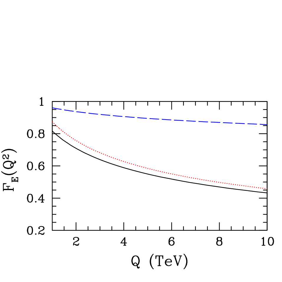
Refer to caption
Figure 12: The Sudakov form-factor for uu-quarks (solid black), tt-quarks (dotted red) and electrons (dashed blue) at μ=MZ\mu=M_{Z} for mH=200m_{H}=200 GeV.
Refer to caption
Figure 13: The Sudakov form-factor for uu-quarks (solid black), tt-quarks (dotted red) and electrons (dashed blue) at μ=30\mu=30 GeV for mH=200m_{H}=200 GeV.
Refer to caption
Figure 14: The electroweak contribution to the Sudakov form-factor (as a percentage change) for uu-quarks (solid black), tt-quarks (dotted red) and electrons (dashed blue) at μ=30\mu=30 GeV for mH=200m_{H}=200 GeV.

FEF_{E} is normalized to unity in the absence of radiative corrections. Radiative corrections for electrons are about 7% at 2 TeV, and μ=MZ\mu=M_{Z}, increasing to about 8% for μ=30\mu=30 GeV due to the QED running below MZM_{Z}. The corrections for quarks are much larger, 15% for the tt-quark, and 30% for the uu-quark at μ=MZ\mu=M_{Z}, increasing to 40% and 50%, respectively, at μ=30\mu=30 GeV. There is also a significant difference between the results for tt- and uu-quarks, arising from power corrections which depend on mt/MW,Zm_{t}/M_{W,Z} and Higgs corrections which depend on the Yukawa coupling gtg_{t}. The bulk of the difference is due to the power corrections, the gtg_{t} terms are less than 1%.55 5 Note that the Higgs corrections do not have the 𝖫Q\mathsf{L}_{Q} enhancement that is present for the gauge bosons. The corrections for the four-quark operators needed for realistic processes are bigger, with corrections even to color singlet processes being greater than 20%. The radiative corrections are large enough that resummation is necessary to get an accurate prediction for the partonic cross-sections. We have shown how one can perform the resummation using EFT methods. Previous computations ciafaloni; fadin; kps; fkps; jkps; jkps4; beccaria; dp1; dp2; hori; beenakker; dmp; pozzorini; js have done the resummation using infrared evolution equations fadin. The EFT method allows one to include mass effects as well as Higgs corrections in a systematic way, which have not been included previously. It also handles the cross-over between the S​U​(3)×S​U​(2)×U⁡(1)SU(3)\times SU(2)\times U(1) and the S​U​(3)×U⁡(1)SU(3)\times U(1) gauge theories above and below the weak interaction symmetry breaking scale, including the effects of unequal WW and ZZ masses. The infrared evolution method uses a conjectured form for this cross-over with equal WW and ZZ masses. The extension of previous results to massive external particles is currently being studied by other groups using a method-of-regions analysis jantzentalk.

RK was supported by an LHC theory fellowship from the NSF.

Appendix A Analytic Regulator Dependence of Collinear Graphs

The nn-collinear contribution Eq. (38) can be written as

In\displaystyle I_{n} =\displaystyle= αs4​πCFc(μ)γμ[2​ηδ​ϵ+2​ηδlogμ2M2+1−ρϵ2\displaystyle\frac{\alpha_{s}}{4\pi}C_{F}c(\mu)\gamma^{\mu}\Biggl[\frac{2\eta}{\delta\epsilon}+\frac{2\eta}{\delta}\log\frac{\mu^{2}}{M^{2}}+\frac{1-\rho}{\epsilon^{2}} (148)
+1ϵ​(2+(1+ρ)​log⁡ν1−p2−−(1−ρ)​log⁡ν22μ2)\displaystyle+\frac{1}{\epsilon}\biggl(2+(1+\rho)\log\frac{\nu_{1}^{-}}{p_{2}^{-}}-(1-\rho)\log\frac{\nu_{2}^{2}}{\mu^{2}}\biggr)
+2+2​log⁡μ2M2−(1−ρ)​log⁡μ2M2​log​ν22μ2\displaystyle+2+2\log\frac{\mu^{2}}{M^{2}}-(1-\rho)\log\frac{\mu^{2}}{M^{2}}\log\frac{\nu_{2}^{2}}{\mu^{2}}
+(1+ρ)​log⁡μ2M2​log​ν1−p2−−12​(1−ρ)​log2​μ2M2\displaystyle+(1+\rho)\log\frac{\mu^{2}}{M^{2}}\log\frac{\nu_{1}^{-}}{p_{2}^{-}}-\frac{1}{2}(1-\rho)\log^{2}\frac{\mu^{2}}{M^{2}}
+ρ​π212−5​π212],\displaystyle+\frac{\rho\pi^{2}}{12}-\frac{5\pi^{2}}{12}\Biggr]\,,

where

η=1r1−r2,ρ=r1+r2r1−r2.\displaystyle\eta=\frac{1}{r_{1}-r_{2}}\,,\qquad\rho=\frac{r_{1}+r_{2}}{r_{1}-r_{2}}\,. (149)

The n¯\bar{n}-collinear contribution is given by Eq. (148) with η→−η\eta\to-\eta, ρ→−ρ\rho\to-\rho, ν2→ν1\nu_{2}\to\nu_{1}, ν1−/p2−→ν2+/p1+\nu_{1}^{-}/p_{2}^{-}\to\nu_{2}^{+}/p_{1}^{+}. The dependence on r1,2r_{1,2} and ν1,2\nu_{1,2} is additional scheme dependence introduced by the analytic regulator. The sum of the nn-collinear and n¯\bar{n}-collinear contributions simplifies greatly, and gives Eq. (45) on using ν1−=ν12/p1+\nu_{1}^{-}=\nu_{1}^{2}/p_{1}^{+}, ν2+=ν22/p2−\nu_{2}^{+}=\nu_{2}^{2}/p_{2}^{-}. In particular, the η\eta and ρ\rho terms cancel between the two contributions. The relevant relations are

[log⁡ν1−p2−+log⁡ν22μ2]−[log⁡ν2+p1++log⁡ν12μ2]\displaystyle\left[\log\frac{\nu_{1}^{-}}{p_{2}^{-}}+\log\frac{\nu_{2}^{2}}{\mu^{2}}\right]-\left[\log\frac{\nu_{2}^{+}}{p_{1}^{+}}+\log\frac{\nu_{1}^{2}}{\mu^{2}}\right] =\displaystyle= log⁡ν1−​ν22​p1+ν2+​ν12​p2−\displaystyle\log\frac{\nu_{1}^{-}\nu_{2}^{2}p_{1}^{+}}{\nu_{2}^{+}\nu_{1}^{2}p_{2}^{-}}
=\displaystyle= 0,\displaystyle 0\,,
[log⁡ν1−p2−−log⁡ν22μ2]+[log⁡ν2+p1+−log⁡ν12μ2]\displaystyle\left[\log\frac{\nu_{1}^{-}}{p_{2}^{-}}-\log\frac{\nu_{2}^{2}}{\mu^{2}}\right]+\left[\log\frac{\nu_{2}^{+}}{p_{1}^{+}}-\log\frac{\nu_{1}^{2}}{\mu^{2}}\right] =\displaystyle= log⁡ν1−​ν2+​μ4p1+​p2−​ν12​ν22\displaystyle\log\frac{\nu_{1}^{-}\nu_{2}^{+}\mu^{4}}{p_{1}^{+}p_{2}^{-}\nu_{1}^{2}\nu_{2}^{2}} (150)
=\displaystyle= −2​𝖫Q.\displaystyle-2\mathsf{L}_{Q}\,.

The identities Eq. (150) do not make any assumptions about the values of ν12\nu_{1}^{2} and ν22\nu_{2}^{2}, which need not be equal.

It is convenient to use the special case of Eq. (148) with ρ=η=0\rho=\eta=0 to define the n,n¯n,\bar{n}-collinear contributions. This form is given by using the analytic regulator followed by the limit r2=−r1r_{2}=-r_{1}, r1→∞r_{1}\to\infty, and gives

In\displaystyle I_{n} =\displaystyle= αs4​πCFc(μ)γμ[1ϵ2+1ϵ(2+logν1−p2−−logν22μ2)\displaystyle\frac{\alpha_{s}}{4\pi}C_{F}c(\mu)\gamma^{\mu}\Biggl[\frac{1}{\epsilon^{2}}+\frac{1}{\epsilon}\biggl(2+\log\frac{\nu_{1}^{-}}{p_{2}^{-}}-\log\frac{\nu_{2}^{2}}{\mu^{2}}\biggr) (151)
+2+2​log⁡μ2M2−log⁡μ2M2​log⁡ν22μ2\displaystyle+2+2\log\frac{\mu^{2}}{M^{2}}-\log\frac{\mu^{2}}{M^{2}}\log\frac{\nu_{2}^{2}}{\mu^{2}}
+logμ2M2logν1−p2−−12log2μ2M2−5​π212],\displaystyle+\log\frac{\mu^{2}}{M^{2}}\log\frac{\nu_{1}^{-}}{p_{2}^{-}}-\frac{1}{2}\log^{2}\frac{\mu^{2}}{M^{2}}-\frac{5\pi^{2}}{12}\Biggr]\,,

which has no 1/δ1/\delta singularities. This form is similar to the value obtained in Ref. zerobin using a rapidity regulator.

Appendix B Parameter Integrals

B.1 Fermions

fF​(z)\displaystyle f_{F}(z) =\displaystyle= 2​∫01d​x​1−xx​log⁡(1−x+z​x21−x)\displaystyle 2\int_{0}^{1}{{{\rm d}}x}\frac{1-x}{x}\log\left(\frac{1-x+zx^{2}}{1-x}\right) (152)
=\displaystyle= 2+(1z−2)​log⁡(z)+2​1−4​zz​tanh−1⁡1−4​z\displaystyle 2+\left(\frac{1}{z}-2\right)\log(z)+\frac{2\sqrt{1-4z}}{z}\tanh^{-1}\sqrt{1-4z}
+12​log2⁡(z)−2​(tanh−1⁡1−4​z)2\displaystyle+\frac{1}{2}\log^{2}(z)-2\left(\tanh^{-1}\sqrt{1-4z}\right)^{2}
hF​(z)\displaystyle h_{F}(z) =\displaystyle= −∫01dx{2(1−x)log(1−x+z​x21−x)\displaystyle-\int_{0}^{1}{\rm d}x\Biggl\{2(1-x)\log\left(\frac{1-x+zx^{2}}{1-x}\right) (153)
+4​z​x​(1−x2)1−x+z​x2}\displaystyle+\frac{4zx(1-x^{2})}{1-x+zx^{2}}\Biggr\}
=\displaystyle= 92+3z+[32​z2−3]​log⁡(z)\displaystyle\frac{9}{2}+\frac{3}{z}+\left[\frac{3}{2z^{2}}-3\right]\log(z)
+(3−6​z−12​z2)z2​1−4​z​tanh−1⁡(1−4​z)\displaystyle+\frac{\left(3-6z-12z^{2}\right)}{z^{2}\sqrt{1-4z}}\tanh^{-1}(\sqrt{1-4z})
h~F​(z)\displaystyle\tilde{h}_{F}(z) =\displaystyle= −∫01dx{(1−x)log(1−x+x2​z1−x)\displaystyle-\int_{0}^{1}{{\rm d}}x\ \Biggl\{(1-x)\log\left(\frac{1-x+x^{2}z}{1-x}\right)
−2​z​x​(1−x)​(2−x)1−x+z​x2}\displaystyle-\frac{2zx(1-x)(2-x)}{1-x+zx^{2}}\Biggr\}
=\displaystyle= −154+32​z−[3z−34​z2−32]​log⁡(z)\displaystyle-\frac{15}{4}+\frac{3}{2z}-\left[\frac{3}{z}-\frac{3}{4z^{2}}-\frac{3}{2}\right]\log(z)
+[1−4​z​(3−6​z)2​z2]​tanh−1⁡(1−4​z)\displaystyle+\left[\frac{\sqrt{1-4z}\left(3-6z\right)}{2z^{2}}\right]\tanh^{-1}(\sqrt{1-4z})

B.2 Scalars

fS​(z)\displaystyle f_{S}(z) =\displaystyle= ∫01d​x​(2−x)x​log⁡1−x+z​x21−x\displaystyle\int_{0}^{1}{{{\rm d}}x}\frac{(2-x)}{x}\log\frac{1-x+zx^{2}}{1-x} (155)
=\displaystyle= 1−(1−12​z)​log⁡(z)\displaystyle 1-\left(1-\frac{1}{2z}\right)\log(z)
+1−4​zz​tanh−1⁡(1−4​z)\displaystyle+\frac{\sqrt{1-4z}}{z}\tanh^{-1}(\sqrt{1-4z})
+12​log2​z−2​(tanh−1⁡1−4​z)2\displaystyle+\frac{1}{2}\log^{2}z-2\left(\tanh^{-1}\sqrt{1-4z}\right)^{2}
hS​(z)\displaystyle h_{S}(z) =\displaystyle= ∫01dx{(3x2−6x+4)log(1−x+z​x21−x)\displaystyle\int_{0}^{1}{\rm d}x\Biggl\{(3x^{2}-6x+4)\log\left(\frac{1-x+zx^{2}}{1-x}\right) (156)
−z​x​(1−x)​(2−x)21−x+z​x2}\displaystyle\qquad-\frac{zx(1-x)(2-x)^{2}}{1-x+zx^{2}}\Biggr\}
=\displaystyle= 32−1z+[32​z−12​z2]​log⁡(z)\displaystyle\frac{3}{2}-\frac{1}{z}+\left[\frac{3}{2z}-\frac{1}{2z^{2}}\right]\log(z)
+[1−4​zz2​(z−1)]​tanh−1⁡(1−4​z)\displaystyle+\left[\frac{\sqrt{1-4z}}{z^{2}}\left(z-1\right)\right]\tanh^{-1}(\sqrt{1-4z})
h~S​(z)\displaystyle\tilde{h}_{S}(z) =\displaystyle= =−∫01dxz​x31−x+z​x2\displaystyle=-\int_{0}^{1}{\rm d}x\frac{zx^{3}}{1-x+zx^{2}} (157)
=\displaystyle= −12−1z+[12​z−12​z2]​log⁡(z)\displaystyle-\frac{1}{2}-\frac{1}{z}+\left[\frac{1}{2z}-\frac{1}{2z^{2}}\right]\log(z)
+[3​z−1z2​1−4​z]​tanh−1⁡(1−4​z)\displaystyle+\left[\frac{3z-1}{z^{2}\sqrt{1-4z}}\right]\tanh^{-1}(\sqrt{1-4z})

For 4​z≥14z\geq 1, the results can be analytically continued using 1−4​z→i​4​z−1\sqrt{1-4z}\to i\sqrt{4z-1} and tanh−1⁡(1−4​z)→i​tan−1⁡(4​z−1)\tanh^{-1}(\sqrt{1-4z})\to i\tan^{-1}(\sqrt{4z-1}). In each integral, the factors of ii cancel, and the function remains real.

References

  • (1) M. Ciafaloni, P. Ciafaloni and D. Comelli, Phys. Rev. Lett. 84, 4810 (2000).
  • (2) P. Ciafaloni and D. Comelli, Phys. Lett. B 446, 278 (1999); Phys. Lett. B 476, 49 (2000).
  • (3) V. S. Fadin, L. N. Lipatov, A. D. Martin and M. Melles, Phys. Rev. D 61, 094002 (2000).
  • (4) J. H. Kuhn, A. A. Penin and V. A. Smirnov, Eur. Phys. J. C 17, 97 (2000).
  • (5) B. Feucht, J. H. Kuhn, A. A. Penin and V. A. Smirnov, Phys. Rev. Lett. 93, 101802 (2004).
  • (6) B. Jantzen, J. H. Kuhn, A. A. Penin and V. A. Smirnov, Phys. Rev. D 72, 051301 (2005) [Erratum-ibid. D 74, 019901 (2006)].
  • (7) B. Jantzen, J. H. Kuhn, A. A. Penin and V. A. Smirnov, Nucl. Phys. B 731, 188 (2005) [Erratum-ibid. B 752, 327 (2006)].
  • (8) M. Beccaria, F. M. Renard and C. Verzegnassi, Phys. Rev. D 63, 053013 (2001).
  • (9) A. Denner and S. Pozzorini, Eur. Phys. J. C 18, 461 (2001).
  • (10) A. Denner and S. Pozzorini, Eur. Phys. J. C 21, 63 (2001).
  • (11) M. Hori, H. Kawamura and J. Kodaira, Phys. Lett. B 491, 275 (2000).
  • (12) W. Beenakker and A. Werthenbach, Nucl. Phys. B 630, 3 (2002).
  • (13) A. Denner, M. Melles and S. Pozzorini, Nucl. Phys. B 662, 299 (2003).
  • (14) S. Pozzorini, Nucl. Phys. B 692, 135 (2004).
  • (15) B. Jantzen and V. A. Smirnov, Eur. Phys. J. C 47, 671 (2006).
  • (16) A. H. . Mueller, Perturbative Quantum Chromodynamics, World Scientific, Singapore, 1989.
  • (17) C. W. Bauer, S. Fleming and M. E. Luke, Phys. Rev. D 63, 014006 (2001).
  • (18) C. W. Bauer, S. Fleming, D. Pirjol and I. W. Stewart, Phys. Rev. D 63, 114020 (2001); C. W. Bauer and I. W. Stewart, Phys. Lett. B 516, 134 (2001); C. W. Bauer, D. Pirjol and I. W. Stewart, Phys. Rev. D 65, 054022 (2002).
  • (19) J. Y. Chiu, F. Golf, R. Kelley and A. V. Manohar, arXiv:0709.2377 [hep-ph].
  • (20) J. Y. Chiu, F. Golf, R. Kelley and A. V. Manohar, in preparation.
  • (21) M. E. Luke, A. V. Manohar and I. Z. Rothstein, Phys. Rev. D 61, 074025 (2000).
  • (22) J. C. Collins, Phys. Rev. D 22, 1478 (1980).
  • (23) A. H. Mueller, Phys. Rev. D 20, 2037 (1979).
  • (24) A. Sen, Phys. Rev. D 24, 3281 (1981).
  • (25) A. V. Manohar, Phys. Rev. D 68, 114019 (2003).
  • (26) A. V. Manohar, Phys. Rev. D 56, 230 (1997).
  • (27) A. V. Manohar, arXiv:hep-ph/9606222.
  • (28) A. V. Manohar and I. W. Stewart, Phys. Rev. D 76, 074002 (2007).
  • (29) C. W. Bauer and A. V. Manohar, Phys. Rev. D 70, 034024 (2004).
  • (30) A. V. Manohar, Phys. Lett. B 633, 729 (2006).
  • (31) M. Beneke and T. Feldmann, Nucl. Phys. B 685, 249 (2004).
  • (32) V. A. Smirnov and E. R. Rakhmetov, Theor. Math. Phys. 120, 870 (1999) [Teor. Mat. Fiz. 120, 64 (1999)].
  • (33) S. Moch, J. A. M. Vermaseren and A. Vogt, Nucl. Phys. B 688, 101 (2004).
  • (34) A. K. Leibovich, Z. Ligeti and M. B. Wise, Phys. Lett. B 564, 231 (2003).
  • (35) A. V. Manohar and M. B. Wise, Heavy Quark Physics, Cambridge University Press (Cambridge, 2000).
  • (36) S. Fleming, A. H. Hoang, S. Mantry and I. W. Stewart, arXiv:hep-ph/0703207; arXiv:0711.2079 [hep-ph].
  • (37) E. E. Jenkins and A. V. Manohar, Phys. Lett. B 255, 558 (1991); Phys. Lett. B 281, 336 (1992).
  • (38) A. H. Hoang and A. V. Manohar, Phys. Lett. B 483, 94 (2000).
  • (39) C. W. Bauer, A. V. Manohar and M. B. Wise, Phys. Rev. Lett. 91, 122001 (2003), C. W. Bauer, C. Lee, A. V. Manohar and M. B. Wise, Phys. Rev. D 70, 034014 (2004), C. W. Bauer and M. D. Schwartz, Phys. Rev. Lett. 97, 142001 (2006), M. Trott, Phys. Rev. D 75, 054011 (2007).
  • (40) B. Jantzen, arXiv:0709.2311 [hep-ph].