�
�
Random sampling of plane partitions
abstract.
This article presents uniform random generators of plane partitions according to the size (the number of cubes in the 3D interpretation). Combining a bijection of Pak with the method of Boltzmann sampling, we obtain random samplers that are slightly superlinear: the complexity is in approximate-size sampling and in exact-size sampling (under a real-arithmetic computation model). To our knowledge, these are the first polynomial-time samplers for plane partitions according to the size (there exist polynomial-time samplers of another type, which draw plane partitions that fit inside a fixed bounding box). The same principles yield efficient samplers for -boxed plane partitions (plane partitions with two dimensions bounded), and for skew plane partitions. The random samplers allow us to perform simulations and observe limit shapes and frozen boundaries, which have been analysed recently by Cerf and Kenyon for plane partitions, and by Okounkov and Reshetikhin for skew plane partitions.
Introduction
Plane partitions, originally introduced by A. Young [30], constitute a natural generalisation of integer partitions in the plane, as they consist of a matrix of integers that are non-increasing in both dimensions (whereas an integer partition is an array of non-increasing integers). In addition, they also have a nice interpretation in 3D-space as a heap of cubes (see Figure 2). Plane partitions have motivated a huge literature in numerous fields of mathematics [1, 11, 12, 19, 29] and statistical physics [16, 27], and have provided crucial insight for solving challenging problems in combinatorics [31], see [2] for a detailed historical account. The problem of enumerating plane partitions was solved by MacMahon [15], who proved the beautiful formula
| (1) |
for the generating function. The simplicity of the formula asks for a combinatorial interpretation. A first direct bijective proof has been given by Krattenthaler [13]. The principle is inspired by the seminal bijection of Novelli-Pak-Stoyanovskii [21] giving an interpretation of the hook-length formula. In [13], Krattenthaler also discusses as application of his bijection a polynomial-time algorithm for the random generation of plane partitions in a given box. Upon looking at the heap of cubes in the direction, this task is equivalent to sampling tilings of a hexagon of side lengths by rhombi; there also exist random samplers for such tilings, which rely either on “coupling from the past principles” [26] or on “determinant algorithms” [28]. In contrast, we are interested here in sampling plane partitions uniformly at random with respect to the size, defined as the sum of the matrix entries. For this purpose, we use another bijective interpretation of MacMahon’s formula recently given by Pak [24].
Let us briefly mention the motivations for having a random sampler of plane partitions according to the size. The size is a natural parameter, as it corresponds to the volume of the plane partition (number of cubes) in the 3D interpretation. Recently, several authors have studied the statistical properties of plane partitions with respect to the size. In particular, under fixed-size distribution, Mutafchiev [18] has shown a limit law for the maximal entry, and Cerf and Kenyon [3] have determined the asymptotic shape (the asymptotic shape in the boxed framework —hexagon tilings— is due to Cohn, Larsen, and Propp [4]). Even more recently, Okounkov and Reshetikhin, using a method based on Schur processes, have rediscovered the limit shape of Cerf and Kenyon [22]. They have studied in a subsequent article [23] the local correlations and limit shapes for plane partitions under a mixed model: the plane partition is constrained to a 2-coordinate box and is drawn under the Boltzmann model with respect to the size. (We will also describe random samplers for this mixed model.) In addition, physicists have developed new models relying on plane partitions, giving rise to a simplified version of the 3-dimensional models of lattice vesicles [14]. Plane partitions are also related to the 3-dimensional Ising model in the cubic lattice [3]. In general, physicists are interested in checking experimentally or conjecturing some limit properties of these models, by generating very large random objects.
For this purpose, this paper introduces efficient samplers for plane partitions. Our approach combines methods from bijective combinatorics and symbolic combinatorics. Precisely, a minor reformulation of Pak’ bijection maps a multiset of integer pairs (the class is denoted by ) to a plane partition with the same size. (Since the class has generating function , this gives a direct proof of (1).) Our aim here is to take advantage of this bijection for random sampling. Indeed Pak’s bijection reduces the task of finding a sampler for plane partitions to the task of finding a sampler for . As the class has an explicit simple combinatorial decomposition, it is amenable to random sampling methods from symbolic combinatorics. By now there is the recursive method [20, 9] based on the counting sequences and Boltzmann samplers based on the generating functions, as introduced in [5] and further developed in [6]. We adopt here the framework of Boltzmann samplers, which tend to be more efficient as they avoid the costly precomputations of coefficients required by the recursive method.
As opposed to the recursive method —which produces exact-size samplers— the probability distribution in Boltzmann sampling is spread over the whole class; precisely an object of size has probability proportional to , where is a fixed real parameter. In particular, as two objects having the same size have equal probability, the probability distribution restricted to a given size is uniform. As we are interested in generating very large plane partitions, the Boltzmann framework is suitable, due to the gain obtained by relaxing the exact-size constraint. The articles [5] and [6] provide a collection of rules for building a sampler for a class admitting a decomposition involving classical constructions. Using these rules, the decomposition of is readily translated into a Boltzmann sampler. This yields, via Pak’s bijection, a Boltzmann sampler for plane partitions. In addition, as the size distribution of plane partitions —under the Boltzmann model— has good concentration properties, it is possible to “tune” the parameter so as to draw objects of size around (or exactly at) a given target value . With the parameter suitably tuned and a rejection loop targeted at the size, we obtain a quasi-linear time approximate-size sampler for plane partitions: for any tolerance-ratio , our sampler draws a plane partition of size in with an expected running . The same principles, with the rejection loop running until a given size is attained, yields an exact-size sampler for plane partitions, with expected running time . To our knowledge, our algorithm is the first exact-size sampler for plane partitions with expected polynomial running time. This allows us to generate objects of size up to in a few minutes on a PC. The same principles (i.e., Pak’s bijection + Boltzmann samplers) yield efficient Boltzmann samplers for -boxed plane partitions (plane partitions whose non-zero entries lie in an () rectangle), which are those considered by Okounkov and Reshetikhin. We obtain for boxed plane partitions an approximate-size sampler with expected running time and an exact-size sampler of expected running time , where is a tolerance-ratio on the size (for approximate-size sampling) and where is the target-size (the dependency in of the asymptotic constants in the big O’s are stated precisely in Theorem 10).
Proving the correct complexity orders of the samplers is the major technical difficulty we have to deal with. At first we have to analyse the expected running time of the Boltzmann sampler for the multiset-class , as well as the size distribution on under the Boltzmann model. All this is done using the Mellin transform. Second, we study the complexity of Pak’s bijection, which depends on a natural length-parameter of a plane partition, which is the maximum hook-length (abscissa+ordinate+1) over all nonzero entries of the matrix. Let us finally mention that, for the sake of simplicity, all complexity results are stated and proved with the notation (upper bound). With little more care one could prove that all the stated complexity results hold in fact with a notation, i.e., an upper and a lower bound.
Outline of the paper. After some definitions in Section 1 about combinatorial classes and plane partitions, we present in Section 2 a slight reformulation (more algorithmic) of Pak’s bijection. The bijection induces a combinatorial isomorphism between the set of plane partitions and the class . Section 3 recalls basic principles of Boltzmann sampling, in particular the sampling rules associated to the constructions appearing in the specification of . The Boltzmann sampler for , as well as , is derived in Section 4, giving rise to Boltzmann samplers for plane partitions and -boxed plane partitions. We explain then briefly how the principles extend to obtain Boltzmann samplers for so-called skew plane partitions. In Section 4.4, using suitable choices of the parameter in the Boltzmann samplers, we obtain efficient samplers for plane partitions targeted exactly or approximately at a given size (precise statements are given in Theorems 9 and 10). The expected running times of the targeted samplers are then analysed in Section 5.
1. Definitions
A combinatorial class is a pair where is a set and is a function from to , called the size function, such that the number of elements of any given size is finite. Using the size function, we can graduate as , where is the set of objects of that have size . In the sequel, we denote by the cardinality of . To each combinatorial class , we associate the generating function .
Two combinatorial classes and are said to be combinatorially isomorphic, , if and only if there exists a one-to-one mapping from to that preserves the size. Let us notice that two classes and are isomorphic if and only if their generating functions are equal.
Here are some classical constructions on combinatorial classes that will be used in this paper. Notations and rules are summarized in Figure 1 (a more general presentation can be found in [8]):
- –
and are atoms of size and .
- –
Disjoint union : the union of two copies of and made disjoint.
- –
Cartesian product : the set of pairs where and .
Given a class not containing empty atoms,
- –
Sequence: is the class of finite sequences of objects of .
- –
Multiset: is the class of finite sets of objects of , with repetitions allowed.
In all these constructions, the size of an object in the composed class is naturally defined as the sum of the sizes of the components (e.g., the size of a sequence is ). Observe that, in a multiset , each element has a multiplicity . Hence, if is a finite set,
| (2) |
| Class | Generating function | Definition |
|---|---|---|
| neutral object of size 0 | ||
| atom of size 1 | ||
| disjoint union | ||
| cartesian product | ||
| a multiset of elements of |
A plane partition (Figure 2) of is a two-dimensional array of non-negative integers that are non-increasing both from left to right and bottom to top and that add up to . In other words,
| (3) |
We denote by the combinatorial class of plane partitions, endowed with the size function . Plane partitions have a natural representation in 3D-space as a heap of cubes with non-increasing height in the direction of the -axis and -axis, see Figure 2. Observe that the size of the plane partition exactly corresponds to the number of cubes in the 3D-representation.
The bounding rectangle of a plane partition is the smallest double range such that for all index pairs outside of . An -boxed plane partition is a plane partition whose bounding rectangle is at most . Equivalently, is null for any such that or . We denote by the class of -boxed plane partitions.

Define the two combinatorial classes and as follows, where denotes the class of sequences of at most elements of .
| (4) | |||||
| (5) |
Classically, is identified with the class of nonnegative integers, so that we can specify with the following simplified notation,
| (6) |
In the next section we explain how Pak’s bijection yields an explicit combinatorial isomorphism between and . For this purpose, we introduce some more terminology. The diagram of an element is a two-dimensional array (with at the bottom left) where is the multiplicity of in (see the first two pictures of Figure 3). The size of is defined as , so that it corresponds to the size of the multiset in . The bounding rectangle of is defined similarly as for plane partitions: it is the smallest double range such that all entries of outside of are zero. The integers and are respectively called the length and the width of . Note that, for fixed integers and , the diagrams of elements in are constrained to have their bounding rectangle . Therefore is called the class of -boxed multisets.
2. Pak’s bijection
In [24], Pak presents a bijection between plane partitions bounded in a shape ( being a Ferrers diagram) and fillings of the entries of with nonnegative integers. We reformulate this bijection as an algorithm, Algorithm 1 below, that realises explicitly the combinatorial isomorphism , see Figure 3 for an example.
for downto do for downto do ;
Proposition 1 (Pak [24]).
Algorithm 1 yields an explicit size-preserving bijection between the class and the class of -boxed plane partitions. In other words, the algorithm realises the combinatorial isomorphism
| (7) |
Proof.
See [24]. ∎

Proposition 2.
Algorithm 1 realises the combinatorial isomorphism
| (8) |
Proof.
Take the limit and in Proposition 1. ∎
3. Boltzmann sampling
Definition 3 (Boltzmann model).
Let be a combinatorial class and its generating function. Given a coherent positive real value of , i.e., chosen within the disk of convergence of ), the Boltzmann model of parameter assigns to any element the following probability,
A Boltzmann sampler for is an algorithm that produces objects of at random under the Boltzmann model. As elements of the same size have the same weight, the probability induced by a Boltzmann sampler on any given size is uniform. The size of the output is a random variable satisfying
Figure 4 shows this probability distribution for plane partitions. When a target size has to be achieved, the idea is to tune the parameter so that (see Section 5).

Figure 5 briefly summarizes how to obtain samplers for the constructions used in the specification of (see details in [6]); the rules can be combined to build a generator for any class specified with these constructions, in particular the class . The sampling rules make use of simple auxiliary generators: generates integers under the geometric law , generates integers under the Poisson law , and generates integers under the positive Poisson law for . Such generators are classically realised by simple iterative loops, the complexity of generating an integer being , see [5] for a discussion.
| where means “ return independent calls to ”. | |
| Define the probability distribution relative to and : | |
| Let be a generator according to this distribution. : ; ; if then for from to do ; for from to do ; for from to do return . |
Proposition 4 (Flajolet et al. [6]).
Given two combinatorial classes and endowed with Boltzmann samplers and , the sampler , as defined in the first entry of Figure 5, is a Boltzmann sampler for . Given a class not containing the empty atom and endowed with a Boltzmann sampler , the samplers , as defined in the second and third entry11 1 We hereby correct an omission in the definition of the sampler for given in [6], namely the test . of Figure 5, are respectively Boltzmann samplers for and for .
From these sampling rules, a class recursively specified from atomic sets in terms of these constructions can be endowed with a Boltzmann sampler . The complexity of generating an object is .
Complexity model. Let us say a few words on the specific real-arithmetic complexity model used for Boltzmann samplers. First, notice that the samplers given in Figure 5 draw integers according to distributions (, , Max_Index) that require the exact values of the generating functions of the classes involved. Hence, such generating functions should be evaluated. The complexity model we adopt, as already defined in [5], relies on the oracle assumption. This assumption allows us to separate the combinatorial complexity of the sampler from the complexity of evaluating the generating functions (there are already some results [25] and work in progress dedicated to the latter issue). Given any combinatorial class specified recursively using the constructions of Figure 5, and given a value within the disk of convergence of , we assume that an oracle provides, at unit cost, the exact values at of the generating functions for all classes intervening in the decomposition of . In practice, we work with a fixed precision (e.g., digits) and precompute the values of generating functions used by the Boltzmann sampler. Finally let us come back to the complexity of drawing an integer under a certain discrete distribution
where the constant are known (if involves exact values of generating functions, the oracle provides the values of ). As discussed in [5], drawing an integer under this distribution is done by a simple loop,
Thus, the cost of drawing is of the order of the value that is finally assigned to . An exception is the case of the geometric law, which is simpler. Indeed, to draw under (with ), it is enough to set , where is uniform in .
Hence, the cost of drawing a geometric law is .
4. Samplers for plane partitions
4.1. Boltzmann sampler for plane partitions
The explicit bijection between and allows us to design a simple Boltzmann sampler for plane partitions, made of two steps: (i) generate a multiset in under the Boltzmann model, (ii) apply Algorithm 1 (Pak’s bijection) to the diagram of the multiset generated.
;
Lemma 5.
Given , the generator —as defined in Algorithm 3— is a Boltzmann sampler for .
Proof.
Since Pak’s bijection preserves the size, Algorithm 4 is a Boltzmann sampler for plane partitions.
Figure 6 shows computation times22 2 Computations have been performed on a Mac OS X Power PC G4 1,42GHz, with 1GB of RAM and 512 kB of cache. of for sizes up to : the first line gives the time of generation of the multiset () and the second line gives the computation time of Pak’s bijection. The sampler has been implemented in Maple and the bijection in OCaml. As we can see, the complexity is dominated by Pak’s bijection for objects of large size. This is confirmed by the analysis to be given in Section 5: the complexity of drawing a multiset of size around is of order , while the expected running time of Pak’s bijection applied to a random multiset of size is of order . Figure 7 shows two large plane partitions generated by for close to 1, and .
| approx. size | ||||||
|---|---|---|---|---|---|---|
| generation | sec. | sec. | 2-3 sec. | sec. | sec. | |
| Pak’s transform | sec. | sec. | sec. | 20-30 sec. | 8-9 min |


4.2. Boltzmann sampler for -boxed plane partitions
According to the equivalence with the definition in terms of diagrams, an element of is a multiset of pairs , with and , each element having size . The set of such pairs being finite, Equation (2) yields
| (9) |
Lemma 6.
Given , the generator —as defined in Algorithm 5— is a Boltzmann sampler for .
for to do for to do ;
Again, since Pak’s bijection preserves the size, the following generator is a Boltzmann sampler for -boxed plane partitions.
4.3. Extension to skew plane partitions
We consider here a natural generalisation of -boxed plane partitions, called -boxed skew plane partitions. A -boxed skew plane partition is given by an index-domain such that is obtained from by removing rectangles of the form , with and . Each truncation by a smaller rectangle makes an outer corner appear in the index domain (e.g., the partition of Figure 8 has 2 outer corners).
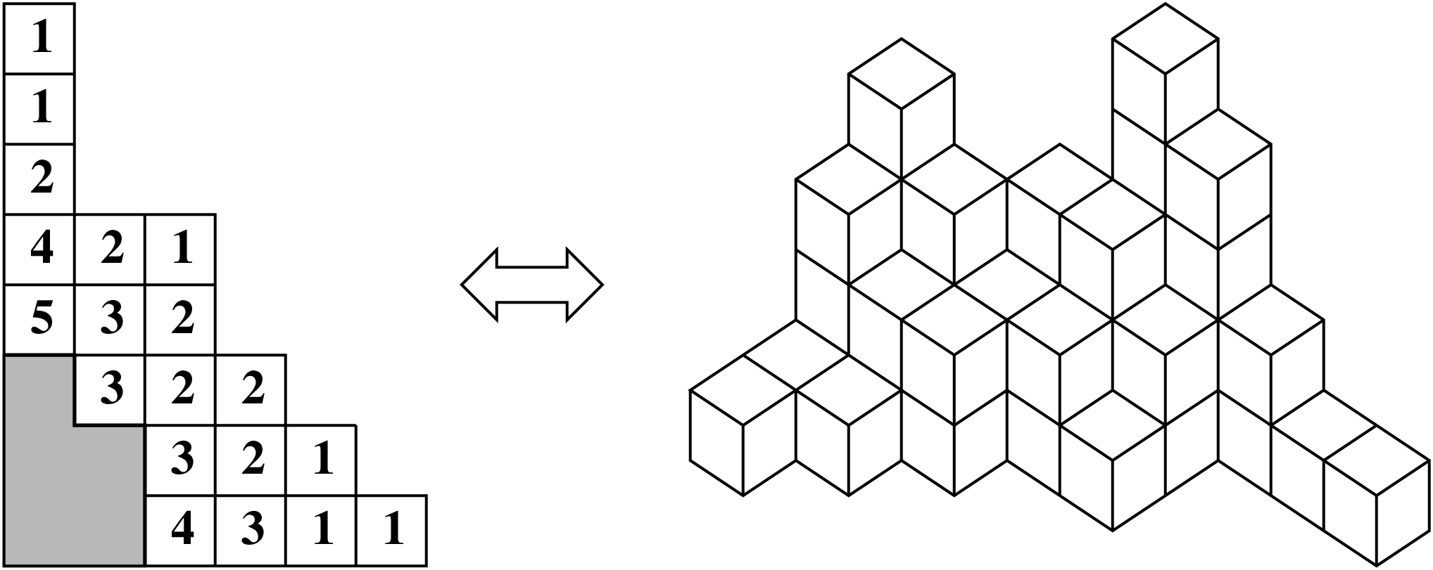
Let us denote by the class of all such partitions for a given domain . For this new class of partitions, we need to define the hook-length of a pair in the domain . Let be the minimum abscissa such that and the minimum ordinate such that . The hook-length of in is then , which is exactly when is . In [24], Pak’s bijection is most generally described for skew plane partitions, which leads to the following combinatorial isomorphism:
The Boltzmann sampler for -boxed plane partitions extends directly to a Boltzmann sampler for skew plane partitions as follows: to sample a diagram, draw the value at each point in according to a geometric law of parameter ; then apply Algorithm 1 (Pak’s bijection) to the multiset generated, with the difference that the domain scanned by is .
Okounkov and Reshetikhin [23] have studied the limit shape of a skew plane partition under the Boltzmann distribution, with the Boltzmann parameter tending to . If the lengths of the rectangles are of order , some interesting phenomena are to be observed regarding the typical shape of a random skew plane partition. Using a technique based on Schur processes, the authors of [23] provide a precise analysis of these phenomena. They prove that the (rescaled) limit shape of a skew plane partition has a frozen boundary that satisfies explicit equations, and they classify the non-smooth points of the boundary as turning points and cusps. Turning points always appear, even for a boxed domain ; they correspond to points of tangency of the frozen boundary with the delimiting 3D-box . If the index domain has outer corners, some cusp points possibly appear at each of the outer corners.
Our random sampler for skew plane partitions makes it possible to perform simulations and observe these asymptotic phenomena. Figure 9(a) shows a -boxed plane partition of size 999,400. A frozen boundary appears that meets the delimiting 3D-box in a tangential way (these points of tangency are precisely the turning points in the terminology of Okounkov and Reshetikhin). And Figure 9(b) shows a skew plane partition of size on the index-domain , which has an outer corner at ; accordingly a cusp point appears on the boundary of the limit shape at the point above .
Note that the typical shape of a large unconstrained random plane partition, as shown in Figure 7, has different features: there are 3 “legs” —one in each axis-direction— whose lengths tend to infinity even when the plane partition is rescaled to have unit volume (which essentially corresponds to rescaling by a factor in each dimension).


4.4. Samplers targeted around a given size
Given a class , an exact-size sampler is a procedure that, for any given (called the target-size), outputs an object of uniformly at random. An approximate-size sampler is a procedure that, for any given and (called the tolerance-ratio), outputs an object of of size in and such that two objects of the same size have the same chance to be drawn (hence the distribution induced on each size is uniform).
Such procedures are easily obtained if is endowed with a Boltzmann sampler . Fix a suitable value of and repeat calling until the size is in the desired size-range ; for exact-size sampling and for approximate-size sampling. The exact-size sampler and approximate-size sampler defined in this way are denoted and , respectively.
In general one chooses so that the expected size of the output of —which satisfies as proved in [5]— is equal to , or at least is asymptotically equal to , that is, one looks for an exact or an approximate solution of the so-called target-size equation:
| (10) |
As we show in Section 5 the expected size of the output of satisfies
where is the Riemann zeta function, so a suitable value of the parameter to reach a target-size is , since ; and we show in Section 5 that the expected size of the output of satisfies
so a suitable value of the parameter to reach target-size is .
Lemma 7 (Targeted samplers for the multiset class ).
Define
Then, under the oracle assumption, the expected running time of is ; and, for fixed , the expected running time of is as , the constant in the big being independent of 33 3 Precisely, for each fixed there is such that the running time is at most for , where the constant is independent of ..
In view of stating the expected running times of the targeted samplers for -boxed multisets, we define the following functions
Lemma 8 (Targeted samplers for -boxed multisets).
Define
Then, for , the expected running time of is equivalent to as . For fixed , the expected running time of converges to the constant as .
Theorem 9 (Targeted samplers for plane partitions).
For , define the algorithm as the procedure that calls and applies Algorithm 1 (Pak’s bijection) to the generated diagram.
Then is an exact-size sampler for plane partitions, of expected running time .
For and , define as the algorithm that calls and applies Algorithm 1 to the generated diagram. Then is an approximate-size sampler for plane partitions, of expected running time as (under fixed ), the asymptotic constant in the big not depending on .
The proofs of the expected running times announced in Theorem 9 and Theorem 10 (given next) are delayed to Section 5.
In view of stating the expected running times of the targeted samplers for -boxed plane partitions, we define the following function
Theorem 10 (Targeted samplers for -boxed Plane Partitions).
For , define as the algorithm that calls and applies Algorithm 1 (Pak’s bijection) to the generated diagram.
Then is an exact-size sampler for -boxed plane partitions, of expected running time equivalent to as .
For and , define as the algorithm that calls and applies Algorithm 1 to the generated diagram.
Then is an approximate-size sampler for -boxed plane partitions, of expected running time equivalent to the constant as (under fixed ).
Let us mention that the targeted samplers for -boxed plane partitions are easily extended to the framework of -boxed skew plane partitions. For a fixed admissible index-domain , the appropriate value to reach a target size exactly (or approximately) is , where is the cardinality of .
Another important remark is that the value works well in the asymptotic regime, that is, when . If not in the asymptotic regime (say one generates plane partitions of size constrained to a rectangular box ) one has to consider the target-size equation more closely. The generating function for multisets with support in is
Hence the target-size equation —— is
which is to be solved exactly if is not in the asymptotic regime for the domain . (The solution is asymptotically , but the rate of convergence is slow when is large.)
5. Analysis of the complexity
This section is dedicated to proving the expected running times of the random samplers, as stated in Theorem 9 and Theorem 10. Since most of the difficulty is in proving Theorem 9 (unconstrained plane partitions), the proof of Theorem 10 is only given in the very last subsection (Section 5.6) and is kept short.
Recall that the random samplers consist of two steps: generate a diagram under the Boltzmann model until the size is in the desired target-domain, and then apply Algorithm 1 (Pak’s bijection) to the diagram so as to output a random plane partition. Accordingly, the complexity of generation is obtained by adding up the cost of generating a diagram and the cost of Pak’s bijection.
The expected costs of generating diagrams under Boltzmann model are naturally expressed as certain infinite sums, which are best handled by the Mellin transform, recalled next. On the other hand, Pak’s bijection has complexity cubic in a certain parameter called the maximum hook-length, which is the maximal value of the hook-length (abscissa+ordinate+1) over all nonzero entries. Therefore, we need to find the asymptotic order of the maximum hook-length under the uniform distribution at size .
5.1. The Mellin transform
The Mellin transform is a powerful technique to derive asymptotic estimates of expressions involving specific infinite sums, (see [7] for a detailed survey), which occur recurrently in the analysis of our samplers. Given a continuous function defined on , the Mellin transform of is the function
| (11) |
For instance, the Euler Gamma function is the Mellin transform of . If as and as , then is an analytic function defined on the fundamental domain . In addition, is in most cases continuable to a meromorphic function in the whole complex plane (for instance, is continuable to a meromorphic function having its poles at negative integers). In a similar way as the Fourier transform, the Mellin transform is almost involutive, the function being recovered from using the inversion formula
| (12) |
From the inversion formula and the residue theorem, the asymptotic expansion of as can be derived from the poles of on the left of the fundamental domain, the rightmost such pole giving the dominant term of the asymptotic expansion. If is decreasing very fast as , (which occurs in all the series to be analysed next, based on the fact that is decaying fast and is of moderate growth as ), then there holds the following transfer rule [7]: a pole of of order (),
yields a term
in the singular expansion of around . In particular, a simple pole yields a term .
Another fundamental property of the Mellin transform is to factorize sums of a certain form,
| (13) |
5.2. Complexity of the Boltzmann samplers for multisets
In this section, we analyse the complexity of the free Boltzmann sampler for the multiset class , not studying yet the rejection cost when targeting at a certain size-domain. In general, given a combinatorial class for which an explicit Boltzmann sampler is designed, we write for the expected running time of a call to . More generally, we use thereafter the letter as a prefix to denote the expected running time of a random generator. As we are interested in drawing large plane partitions, which requires to let tend to , we analyse the asymptotic order of as . Recall that , with generating function . By definition, the first step of the Boltzmann sampler is to draw an integer under the probability distribution
| (14) |
Under the oracle assumption discussed in Section 3 and described in details in [5], the complexity of drawing is thus of the order of the value that is finally assigned to . Hence the expected running time of drawing is of the same order as the expected value of under the above given distribution.
Lemma 11.
The expectation of under the distribution (14) satisfies
Proof.
Fix . Let be the smallest integer such that , i.e., . Note that for . Hence, for , . And, for ,
Hence, for ,
We obtain thus
which concludes the proof since is as . ∎
Once the integer is drawn, the Boltzmann sampler draws Poisson laws and geometric laws (a call to consists of two calls to geometric laws). Precisely, for each , the number of calls to follows a Poisson law . Since , the expected number of calls to is . In addition, each call to takes constant time, since it consists of two calls to geometric laws. Hence
| (15) |
Lemma 12.
The expected running time of the Boltzmann sampler satisfies
Proof.
By Equation (15), it is enough to show that is as . This is a first instance where the Mellin transform can be successfully applied (more elementary approaches would work in this simple case). Define . Then
The factorization property of the Mellin transform, Equation (13), yields
where is the Riemann zeta function. Since , the factorization property yields . Thus, . It is easily checked that as and as , so that the fundamental domain of is . Hence, to determine the asymptotic behavior of as , we have to find the rightmost poles of such that . The function has a unique pole at with coefficient 1, and the function has its poles at non-positive integers. Hence has a simple pole at , with coefficient , and no other pole for , so that the transfer rule of the Mellin transform yields
The change of variable yields
As a consequence, as . ∎
5.3. Analysis of the size of a multiset in under the Boltzmann model
Given , denote by the random variable giving the size of the output of (which is also the size of a plane partition under the Boltzmann model at ); Figure 4 shows plots of for several values of . As the Boltzmann probability of an object of size is , the expectation and variance of satisfy (see [5] for details):
Lemma 13.
The expectation and variance of the size of a multiset drawn under Boltzmann model satisfy
Proof.
We use once again the Mellin transform to derive the asymptotic estimates. Observe that is the logarithmic derivative of , hence the expression (1) of yields
Define . Then
where . Hence
The function is defined on the fundamental domain . The rightmost pole such that is at , where . As there are no other poles for , the transfer rule yields
Hence the change of variable gives
The variance is treated similarly,
Hence the function satisfies , where . Thus, . The location of the poles of and the transfer rule yields
giving
∎
5.4. Complexity of the targeted samplers for multisets
Recall that the targeted samplers for the multiset class repeat calling the Boltzmann sampler with a suitable value of until the size is in the target domain ; for exact-size sampling and for approximate-size sampling.
Lemma 14.
For , let be the solution of , i.e.,
Define as the probability that the output of has size . For any , define as the probability that the size of the output of is in the range . Then, as , with ; and, for fixed , as .
Proof.
As is solution of , Lemma 13 ensures that as , i.e., there exists such that . Hence Chebyshev’s inequality gives, for any ,
Given the fact that , we have as .
Next we prove the estimate of . Note that
Hence it is enough to obtain the asymptotics of and as , and of as . These have first been found by Wright [29] and later by Meinardus in a more general framework [17] relying on the saddle-point method (a detailed and accessible presentation of the saddle-point method is given in [8, Ch.VIII], partitions are studied in the 6th section of the chapter). We briefly review the main ingredients. To find the asymptotics of as , one applies the Mellin transform techniques to the series , and finds
| (16) |
with an explicit constant, . Define , so and . From (16) we obtain
with . The asymptotics of is easy to obtain. Since , we obtain
with . Finally the asymptotics of has been obtained by Wright [29] using the saddle-point method and the estimate (16). The idea is to use Cauchy’s formula
with the circle of radius centered at as the integration contour. Using the estimate (16) (more precisely one needs the fact that this estimate holds in an open cone centered at and containing the line ), one shows that the main contribution of the integral is on a small arc of around the origin, and obtains
with . Thus, from the estimates of , , and , we find
with . ∎
It is easily checked that the expected running time of a rejection sampler is the expected running time of the sampler times the expected number of calls (which is the inverse of the probability of success), therefore
Since and , we have . Moreover and (for fixed ) by Lemma 14. Hence and , which concludes the proof of Lemma 7.
5.5. Complexity of Pak’s bijection
The aim of this section is to provide an bound on the expected running time of Algorithm 1 for a multiset of size taken uniformly at random. As we will see, the complexity of Algorithm 1 applied to a multiset is expressed in terms of the width and length of the bounding rectangle of . These parameters have been recently studied by Mutafchiev in [18]: using the saddle-point method he shows that the width (similarly the length) after suitable normalization converges weakly to an explicit distribution. Since we are only interested in a big , we only need upper bounds, which are much simpler to show. Therefore we prefer to provide here our own simple self-contained analysis.
For a multiset represented by its diagram, let and be the width and height of the bounding rectangle of . Pak’s bijection scans the double range ; when a square is treated, the squares that are updated are those on the up-right diagonal ; each update of an entry consists of a fixed number of operations involving . The sum of the lengths of the up-right diagonals over the squares of the bounding rectangle is , which is equal to
| (17) |
This quantity is clearly , so that the complexity of Algorithm 1 is cubic in .
We introduce a parameter that will crucially simplify the analysis. Given represented as a diagram, the hook-length of an entry of the diagram is defined as , i.e., is the size of seen as an element of . The maximum hook-length of , denoted by , is the maximum value of the hook-length over all non-zero entries of the diagram of .
Lemma 15.
Given an element in , the complexity of Pak’s bijection applied to is , where is the maximal hook-length of .
Proof.
The maximal hook-length is at least equal to the width and to the height of the bounding rectangle of . Hence the complexity of Pak’s bijection, which is , is also . ∎
Hence, to have a big bound on the expected running time of Pak’s bijection, we need to bound the expected value of for a multiset of size taken uniformly at random. First, for a series with non-negative coefficients and with radius of convergence , we recall the trivial bound
| (18) |
Lemma 16 (expected running time of Pak’s bijection at a fixed size).
For , let be a multiset of size taken uniformly at random. Then the expected running time of Algorithm 1 applied to is .
Proof.
Denote by the expectation of for a multiset of size taken uniformly at random. By Lemma 15, the expected running time of Algorithm 1 under the uniform distribution (on ) at size is . Hence to show the lemma we just have to show that . For , denote by the family of multisets in with maximal hook-length equal to , and denote by the series of . Define
Note that , with the number of plane partitions of size . For , define a -pointed multiset as a multiset where a non-zero entry at hook-length is marked in the diagram of . Note that the series of -pointed multisets is , where the factor counts the possible places to mark an entry and where the factor takes account of the fact that the marked entry is non-zero. Since -pointed multisets form a superfamily of , we have
Let be a constant whose value is to be fixed later, and define . We have
As , the bound (18) ensures that, for ,
Hence
Let . We have
Moreover, according to Lemma 14,
Hence
Taking the constant sufficiently large so that (e.g., ), we obtain
∎
Proposition 17.
For any , the expected running time of satisfies
the asymptotic constant in the big being independent of .
The expected running time of satisfies
5.6. Complexity of the samplers for -boxed plane partitions
By definition (see Algorithm 5), the Boltzmann sampler for -boxed multisets just consists of calls to geometric laws. Giving unit cost to a call to a geometric law, one has
Next, recall that
For , a class is called -singular at if for some constant (the holding in a complex neighbourhood of ) and if is the only singularity of in a disk of the form for some . Note that is -singular for . In [5] it is shown that if is -singular at , then for the probability of being of size under the Boltzmann model at satisfies
| (19) |
And, for fixed , the probability of being in the size-domain under the Boltzmann model at satisfies
| (20) |
Since the expected running time of a rejection sampler is the expected running time of the sampler divided by the probability of success at each attempt, the expected running times of the targeted samplers for satisfy asymptotically
The second step of the targeted samplers for -boxed plane partitions is Algorithm 1 (Pak’s bijection). When , all entries of the rectangle in the diagram of are non-zero with high probability, hence the bounding rectangle of is with high probability. As a consequence, the complexity of Algorithm 1 applied to is with high probability the quantity defined in (17). Hence
which concludes the proof of Theorem 10.
Acknowledgement. The authors would like to thank Philippe Flajolet for his help to analyse the algorithm. The article has also greatly benefited from a discussion with Christian Krattenthaler and from detailed comments of Mireille Bousquet-Mélou and of an anonymous referee on a first manuscript. We finally thank Guénaël Renault for the 3D drawings of plane partitions.
References
- [1] E. A. Bender and D. E. Knuth. Enumeration of plane partitions. J. Combin. Theory Ser. A, 13(1):40–54, 1972.
- [2] David M. Bressoud. Proofs and confirmations: the story of the alternating sign matrix conjecture. Cambridge University Press, New York, NY, USA, 1999.
- [3] R. Cerf and R. Kenyon. The low-temperature expansion of the Wulff crystal in the 3D Ising model. Comm. Math. Phys., 222(1):147–179, 2001.
- [4] H. Cohn, M. Larsen, and J. Propp. The shape of a typical boxed plane partition. New York J. Math., 4:137–166, 1998.
- [5] P. Duchon, P. Flajolet, G. Louchard, and G. Schaeffer. Boltzmann samplers for the random generation of combinatorial structures. Combin. Probab. Comput., 13(4–5):577–625, 2004. Special issue on Analysis of Algorithms.
- [6] P. Flajolet, É. Fusy, and C. Pivoteau. Boltzmann sampling of unlabelled structures. In Proceedings of the 4th Workshop on Analytic Algorithms and Combinatorics, ANALCO’07 (New Orleans), pages 201–211. SIAM, 2007.
- [7] P. Flajolet, X. Gourdon, and P. Dumas. Mellin transforms and asymptotics: Harmonic sums. Theoret. Comput. Sci., 144(1–2):3–58, June 1995.
- [8] P. Flajolet and R. Sedgewick. Analytic combinatorics. Cambridge University Press, 2009.
- [9] P. Flajolet, P. Zimmerman, and B. Van Cutsem. A calculus for the random generation of labelled combinatorial structures. Theoret. Comput. Sci., 132(1-2):1–35, 1994.
- [10] É. Fusy. Uniform random sampling of planar graphs in linear time, 2007. arXiv:0705.1287, to appear in Random Structures Algorithms.
- [11] E. R. Gansner. Matrix correspondences of plane partitions., 1981.
- [12] D. E. Knuth. Permutations, matrices, and generalized Young tableaux. Pacific J. Math., 34:709–727, 1970.
- [13] C. Krattenthaler. Another involution principle-free bijective proof of Stanley’s hook-content formula. J. Combin. Theory Ser. A, 88(1):66–92, 1999.
- [14] J. Ma and E. J. Janse van Rensburg. Rectangular vesicles in three dimensions. J. Phys. A, 38(19):4115–4147, 2005.
- [15] P. A. MacMahon. Memoir on the theory of the partitions of numbers. vi: Partitions in two-dimensional space, to which is added an adumbration of the theory of partitions in three-dimensional space. Phil. Trans. Roy. Soc. London Ser. A, 211:345–373, 1912.
- [16] T. Maeda and T. Nakatsu. Amoebas and instantons. Int. J. Mod. Phys. A, 22:937–984, 2007.
- [17] G. Meinardus. Asymptotische Aussagen über Partitionen. Math. Z., 59:388–398, 1954.
- [18] L. Mutafchiev. The size of the largest part of random plane partitions of large integers. Integers, 6:A13, 2006.
- [19] L. Mutafchiev and E. Kamenov. Asymptotic Formula for the Number of Plane Partitions of Positive Integers. C. R. Acad. Bulgare Sci., 59(4):361–366, 2006.
- [20] A. Nijenhuis and H. S. Wilf. Combinatorial Algorithms. Academic Press, second edition, 1978.
- [21] J.-C. Novelli, I. Pak, and A. V. Stoyanovskii. A direct bijective proof of the hook-length formula. Discrete Math. Theor. Comput. Sci., 1(1):53–67, 1997.
- [22] A. Okounkov and N. Reshetikhin. Correlation function of schur process with application to local geometry of a random 3-dimensional young diagram. J. Amer. Math. Soc., 16(3):581–603, 2003.
- [23] A. Okounkov and N. Reshetikhin. Random skew plane partitions and the pearcey process. Comm. Math. Phys., 269(3), February 2007.
- [24] I. Pak. Hook length formula and geometric combinatorics. Séminaire Lotharingien de Combinatoire, 46:Art. B46f, 13 pp. (electronic), 2001/02.
- [25] C. Pivoteau, B. Salvy, and M. Soria. Boltzmann oracle for combinatorial systems. In Algorithms, Trees, Combinatorics and Probabilities, pages 475–488. Discrete Mathematics and Theoretical Computer Science, 2008. Proceedings of the Fifth Colloquium on Mathematics and Computer Science. Blaubeuren, Germany. September 22-26, 2008.
- [26] J. Propp. Generating random elements of finite distributive lattices. Electron. J. Combin., 4(2), 1997. R15, 12p.
- [27] A. M. Vershik. Statistical mechanics of combinatorial partitions, and their limit configurations. Funct. Anal. Appl., 30(2):90–105, 1996.
- [28] D. B. Wilson. Determinant algorithms for random planar structures. In SODA ’97: Proceedings of the eighth annual ACM-SIAM symposium on Discrete algorithms, pages 258–267, Philadelphia, PA, USA, 1997. Society for Industrial and Applied Mathematics.
- [29] E. M. Wright. Asymptotic partition formulae, i: Plane partitions. Quart. J. Math. Oxford, Ser. 2:177–189, 1931.
- [30] A. Young. On quantitative substitutional analysis. Proc. Lond. Math. Soc., 33:97–146, 1901.
- [31] D. Zeilberger. Proof of the alternating sign matrix conjecture. Electron. J. Combin., 3(2):Research Paper 13, approx. 84 pp. (electronic), 1996. The Foata Festschrift.