A Method for Compressing Parameters in Bayesian Models with Application to Logistic Sequence Prediction Models11
1
This paper appeared as part of Longhai Li’s PhD thesis (Li,
2007).
Longhai Li22 2 Department of Mathematics and Statistics, University of Saskatchewan, Saskatoon, Saskatchewan, S7N5E6, CANADA. Email:longhai@math.usask.ca and Radford M. Neal33 3 Department of Statistics, University of Toronto, Toronto, Ontario, M5S3G3, CANADA. Email: radford@utstat.toronto.edu
Abstract. Bayesian classification and regression with high order interactions is largely infeasible because Markov chain Monte Carlo (MCMC) would need to be applied with a great many parameters, whose number increases rapidly with the order. In this paper we show how to make it feasible by effectively reducing the number of parameters, exploiting the fact that many interactions have the same values for all training cases. Our method uses a single “compressed” parameter to represent the sum of all parameters associated with a set of patterns that have the same value for all training cases. Using symmetric stable distributions as the priors of the original parameters, we can easily find the priors of these compressed parameters. We therefore need to deal only with a much smaller number of compressed parameters when training the model with MCMC. The number of compressed parameters may have converged before considering the highest possible order. After training the model, we can split these compressed parameters into the original ones as needed to make predictions for test cases. We show in detail how to compress parameters for logistic sequence prediction models. Experiments on both simulated and real data demonstrate that a huge number of parameters can indeed be reduced by our compression method.
1 Introduction
In many classification and regression problems, the response variable depends on high-order interactions of “features” (also called “covariates”, “inputs”, “predictor variables”, or “explanatory variables”). Some complex human diseases are found to be related to high-order interactions of susceptibility genes and environmental exposures (Ritchie et. al. 2001). The prediction of the next character in English text is improved by using a large number of preceding characters (Bell, Cleary and Witten 1990). Many biological sequences have long-memory properties.
When the features are discrete, we can employ high-order interactions in classification and regression models by introducing, as additional predictor variables, the indicators for each possible interaction pattern, equal to if the pattern occurs for a subject and otherwise. In this paper we will use “features” for the original discrete measurements and “predictor variables” for these derived variables, to distinguish them. The number of such predictor variables increases exponentially with the order of interactions. The total number of order- interaction patterns with binary (0/1) features is , accordingly we will have predictor variables. A model with interactions of even a moderate order is prohibitive in real applications, primarily for computational reasons. People are often forced to use a model with very small order, say only or , which, however, may omit useful high-order predictor variables.
Besides the computational considerations, classification and regression with a great many predictor variables may “overfit” the data. Unless the number of training cases is much larger than the number of predictor variables the model may fit the noise instead of the signal in the data, with the result that predictions for new test cases are poor. This problem can be solved by using Bayesian modeling with appropriate prior distributions. In a Bayesian model, we use a probability distribution over parameters to express our prior belief about which configurations of parameters may be appropriate. One such prior belief is that a parsimonious model can approximate the reality well. In particular, we may believe that most high-order interactions are largely irrelevant to predicting the response. We express such a prior by assigning each regression coefficient a distribution with mode , such as a Gaussian or Cauchy distribution centered at . Due to its heavy tail, a Cauchy distribution may be more appropriate than a Gaussian distribution to express the prior belief that almost all coefficients of high order interactions are close to , with a very small number of exceptions. Additionally, the priors we use for the widths of Gaussian or Cauchy distributions for higher order interaction should favor small values. The resulting joint prior for all coefficients favors a model with most coefficients close to , that is, a model emphasizing low order interactions. By incorporating such prior information into our inference, we will not overfit the data with an unnecessarily complex model.
However, the computational difficulty with a huge number of parameters is even more pronounced for a Bayesian approach than other approaches, if we have to use Markov chain Monte Carlo methods to sample from the posterior distribution, which is computationally burdensome even for a moderate number of parameters. With more parameters, a Markov chain sampler will take longer for each iteration and require more memory, and may need more iterations to converge or get trapped more easily in local modes. Applying Markov chain Monte Carlo methods to classification and regression with high-order interactions therefore seems infeasible.
In this paper, we show how these problems can be solved by effectively reducing the number of parameters in a Bayesian model with high-order interactions, using the fact that in a model that uses all interaction patterns, from a low order to a high order, many predictor variables have the same values for all training cases. For example, if an interaction pattern occurs in only one training case, all the interaction patterns of higher order contained in it will also occur in only that case and have the same values for all training cases — for that training case and for all others. Consequently, only the sum of the coefficients associated with these predictor variables matters in the likelihood function. We can therefore use a single “compressed” parameter to represent the sum of the regression coefficients for a group of predictor variables that have the same values in training cases. For models with very high order of interactions, the number of such compressed parameters will be much smaller than the number of original parameters. If the priors for the original parameters are symmetric stable distributions, such as Gaussian or Cauchy, we can easily find the prior distributions of these compressed parameters, as they are also symmetric stable distributions of the same type. In training the model with Markov chain Monte Carlo methods we need to deal only with these compressed parameters. After training the model, the compressed parameters can be split into the original ones as needed to make predictions for test cases. Using our method for compressing parameters, one can handle Bayesian regression and classification problems with very high order of interactions in a reasonable amount of time.
This paper will be organized as follows. In Section 2 we describe in general terms the method of compressing parameters, and how to split them to make predictions for test cases. We then apply the method to logistic sequence models in Section 3. There, we will describe the specific schemes for compressing parameters for the sequence prediction models, and use simulated data and real data to demonstrate our method. We draw conclusions and discuss future work in Section 4.
The software package (using R as interface but with most functions written in C) for the method described in this paper is available from http://math.usask.ca/longhai.
2 Our Method for Compressing Parameters
2.1 Compressing Parameters
Our method for compressing parameters is applicable when we can divide the regression coefficients used in the likelihood function into a number of groups such that the likelihood is a function only of the sums over these groups. The groups will depend on the particular training data set. An example of such a group is the regression coefficients for a set of predictor variables that have the same values for all training cases. It may not be easy to find an efficient scheme for grouping the parameters of a specific model. We will describe how to group the parameters for sequence prediction models in Section 3. Suppose the number of such groups is . The parameters in group are denoted by , and the sum of them is denoted by :
| (1) |
We assume that the likelihood function can be written as:
| (2) | |||||
Note that the above ’s are only the regression coefficients for the interaction patterns occurring in training cases. The predictive distribution for a test case may use extra regression coefficients, whose distributions depend only on the priors given relevant hyperparameters.
We need to define priors for the in a way that lets us easily find the priors of the . For this purpose, we assign each a symmetric stable distribution centered at with width parameter . Symmetric stable distributions (Feller 1966) have the following additive property: If random variables are independent and have symmetric stable distributions of index , with location parameters and width parameters , then the sum of these random variables, , also has a symmetric stable distribution of index , with location parameter and width parameter . Symmetric stable distributions exist and are unique for . The symmetric stable distributions with are Cauchy distributions. The density function of a Cauchy distribution with location parameter and width parameter is . The symmetric stable distributions with are Gaussian distributions, for which the width parameter is the standard deviation. Since the symmetric stable distributions with other than or do not have closed form density functions, we will use only Gaussian or Cauchy priors. That is, each parameter has a Gaussian or Cauchy distribution with location parameter and width parameter :
| (3) |
Some may be common for different , but for the moment we denote them individually. We might also treat the ’s as unknown hyperparameters, but again we assume them fixed for the moment.
If the prior distributions for the ’s are as in (3), the prior distribution of can be found using the property of symmetric stable distributions:
| (4) |
Let us denote the density of in (4) by (either a Gaussian or Cauchy), and denote collectively by . The posterior distribution can be written as follows:
| (5) |
where is the training data, and is the marginal probability or density function of .
Since the likelihood function typically depends on in a complicated way, we may have to use some Markov chain sampling method to sample for from distribution (5).
2.2 Splitting Compressed Parameters

After we have obtained samples of , probably using some Markov chain sampling method, we may need to split them into their original components to make predictions for test cases. This “splitting” distribution depends only on the prior distributions, and is independent of the training data . In other words, the splitting distribution is just the conditional distribution of given , whose density function is:
| (6) |
where is the density function of the prior for . Note that is omitted since it is equal to .
As will be discussed in the Section 2.4, sampling from (6) can be done efficiently by a direct sampling method, which does not involve costly evaluations of the likelihood function. We need to use Markov chain sampling methods and evaluate the likelihood function only when sampling for . Figure 1 shows the sampling procedure after compressing parameters, where is a collective representation of , for . When we consider high-order interactions, the number of groups, , will be much smaller than the number of ’s. This procedure is therefore much more efficient than applying Markov chain sampling methods to all the original parameters.
Furthermore, when making predictions for a particular test case, we actually do not need to sample from the distribution (6), of dimension , but only from a derived 1-dimensional distribution, which saves a huge amount of space.
Before discussing how to sample from (6), we first phrase this compressing-splitting procedure more formally in the next section to show its correctness.
2.3 Correctness of the Compressing-Splitting Procedure
The above procedure of compressing and splitting parameters can be seen in terms of a transformation of the original parameters to a new set of parameters containing ’s, as defined in (1), in light of the training data. The posterior distribution (5) of and the splitting distribution (6) can be derived from the joint posterior distribution of the new parameters.
The invertible mappings from the original parameters to the new parameters are shown as follows, for ,
| (7) |
In words, the first original parameters ’s are mapped to themselves (we might use another set of symbols, for example , to denote the new parameters, but here we still use the old ones for simplicity of presentation while making no confusion), and the sum of all ’s, is mapped to . Let us denote the new parameters , for , collectively by , and denote by . (Note that does not include , for . Once we have obtained the samples of and we can use to obtain the samples of .)
The posterior distribution of the original parameters, , is:
| (8) |
By applying the standard formula for the density function of transformed random variables, we can obtain from (8) the posterior distribution of the and :
| (9) |
where the is absolute value of the determinant of the Jacobian matrix, , of the mapping (7), which can be shown to be .
Using the additive property of symmetric stable distributions, which is stated in section 2.1, we can analytically integrate out in , resulting in the marginal distribution :
| (11) | |||||
| (12) |
The conditional distribution of given and can then be obtained as follows:
| (13) | |||||
| (14) |
From the above expression, it is clear that is unrelated to , i.e., , and is independent for different groups. Equation (6) gives this distribution only for one group .
2.4 Sampling from the Splitting Distribution
In this section, we discuss how to sample from the splitting distribution (6) to make predictions for test cases after we have obtained samples of .
If we sampled for all the ’s, storing them would require a huge amount of space when the number of parameters in each group is huge. We therefore sample for conditional on only temporarily, for a particular test case. As will be seen in Section 3, the predictive function needed to make prediction for a particular test case, for example the probability that a test case is in a certain class, depends only on the sums of subsets of ’s in groups. After re-indexing the ’s in each group such that the are those needed by the test case, the variables needed for making a prediction for the test case are:
| (15) |
Note that when , , and when , . The predictive function may also use some sums of extra regression coefficients associated with the interaction patterns that occur in this test case but not in training cases. Suppose the extra regression coefficients need to be divided into groups, as required by the form of the predictive function, which we denote by . The variables needed for making prediction for the test cases are:
| (16) |
In terms of the above variables, the function needed to make a prediction for a test case can be written as
| (17) |
Let us write collectively as , and write as . The integral required to make a prediction for this test case is
| (18) |
The integral over is done by MCMC. We also need to sample for from , which is the prior distribution of given some hyperparameters (from the current MCMC iteration) and can therefore be sampled easily. Finally, we need to sample from , which can be derived from (6), shown as follows:
| (19) |
where and are the priors (either Gaussian or Cauchy) of and , respectively. We can obtain (19) from (6) analogously as we obtained the density of , that is, by first mapping and to a set of new parameters containing and , then integrating away other parameters, using the additive property of symmetric stable distributions. The distribution (19) splits into two components.
When the priors for the ’s are Gaussian distributions, the distribution (19) is also a Gaussian distribution, given as follows:
| (20) |
where and . Since (20) is a Gaussian distribution, we can sample from it by standard methods.
When we use Cauchy distributions as the priors for the ’s, the density function of (19) is:
| (21) |
where , , and is the normalizing constant given below by (23).
When and , the distribution (21) is a t-distribution with degrees of freedom, mean and width , from which we can sample by standard methods. Otherwise, the cumulative distribution function (CDF) of (21) can be shown to be:
| (22) | |||||
where
| (23) | |||||
| (24) | |||||
| (25) | |||||
| (26) |
When , the derivation of (22) uses the equations below from (27) to (29) as follows, where , and we assume ,
| (27) | |||||
| (28) | |||||
| (29) |
When , the derivation of (22) uses the following equations:
| (30) | |||||
| (31) |
Since we can compute the CDF of (21) with (22) explicitly, we can use the inversion method to sample from (21), with the inverse CDF computed by some numerical method. We chose the Illinois method (Thisted 1988, Page 171), which is robust and fairly fast.
When sampling for temporarily for each test case is not desired, for example, when we need to make predictions for a huge number of test cases at a time, we can still apply the above method that splits a Gaussian or Cauchy random variable into two parts times to split into parts. Our method for compressing parameters is still useful because sampling from the splitting distributions uses direct sampling methods, which are much more efficient than applying Markov chain sampling method to the original parameters. However, we will not save space if we take this approach of sampling for all ’s.
3 Application to Sequence Prediction Models
In this section, we show how to compress parameters of logistic sequence prediction models in which states of a sequence are discrete. We will first define this class of models, and then describe the scheme for grouping the parameters. To demonstrate our method, we use a binary data set generated using a hidden Markov model, and a data set created from English text, in which each state has 3 possibilities (consonant, vowel, and others). These experiments show that our compression method produces a large reduction in the number of parameters needed for training the model, when the prediction for the next state of a sequence is based on a long preceding sequence, i.e., a high-order model. We also show that good predictions on test cases result from being able to use a high-order model.
3.1 Bayesian Logistic Sequence Prediction Models

We write a sequence of length as , where takes values from to , for , and takes values from to . We call the historic sequence. For subject we write its historic sequence and response as and . We are interested in modelling the conditional distribution .
An interaction pattern is written as , where can be from to , with meaning that can be any value from to . For example, denotes the pattern that fixes and allows to be any values in their ranges. When all nonzero elements of are equal to the corresponding elements of a historic sequence, , we say that pattern occurs in , or pattern is expressed by , denoted by . We will use the indicator as a predictor variable, whose coefficient is denoted by . For example, is the intercept term. A logistic model assigns each possible value of the response a linear function of the predictor variables. We use to denote the coefficient associated with pattern and used in the linear function for .
For modeling sequences, we consider only the patterns where all zeros (if any) are at the start. Let us denote all such patterns by . We write all coefficients for , i.e., , collectively as . Figure (2) displays for binary sequence of length , for some , placed in a tree-shape.
Conditional on and , the distribution of is defined as
| (32) |
where
| (33) |
In Figure 2, we display the linear functions for each possible combination of on the left column, by linking together all ’s in the summation (33) with lines, from to .
The prior for each is a Gaussian or Cauchy distribution centered at , whose width depends on the order, , of , which is the number of nonzero elements of . There are such width parameters, denoted by . The ’s are treated as hyperparameters, assigned Inverse Gamma prior distributions with some shape and rate parameters, leaving their values to be determined by the data. In summary, the hierarchy of the priors is:
where Inverse-Gamma denotes an Inverse Gamma distribution with density function . We express and in (3.1) so that the mode of the prior is .
3.2 Remarks on the Sequence Prediction Models
The Inverse Gamma distributions have heavy upward tails when is small, and particularly when , they have infinite means. An Inverse Gamma distribution with and small , favors small values around , but still allows to be exceptionally large, as needed by the data. Similarly, the Cauchy distributions have heavy two-sided tails. The absolute value of a Cauchy random variable has infinite mean. When a Cauchy distribution with center and a small width is used as the prior for a group of parameters, such as all ’s of the interaction patterns with the same order in (3.1), a few parameters may be much larger in absolute value than others in this group. As the priors for the coefficients of high-order interaction patterns, the Cauchy distributions can therefore express more accurately than the Gaussian distributions the prior belief that most high-order interaction patterns are useless in predicting the response, but a small number may be important.
It seems redundant to use a for each in (32) since only the differences between matter in (32). A non-Bayesian model could fix one of them, say , all equal to , so as to make the parameters identifiable. However, when , forcing in a Bayesian model will result in a prior that is not symmetric for all , which we may not be able to justify. When , we do require that are all equal to , as there is no asymmetry problem.
Inclusion of other than the highest order is also a redundancy, which facilitates the expression of appropriate prior beliefs. The prior distributions of linear functions of similar historic sequences are positively correlated since they share some common ’s, for example, in the model displayed by Figure 2, and share and . Consequently, the predictive distributions of are similar given similar . By incorporating such a prior belief into our inference, we borrow “statistical strength” for those historic sequences with few replications in the training cases from other similar sequences with more replications, avoiding making an unreasonably extreme conclusion due to a small number of replications.
3.3 Specifications of the Priors and Computation Methods
3.3.1 The Priors for the Hyperprameters
We fix at for the Cauchy models and for the Gaussian models. For , the prior for is Inverse Gamma, where and are:
| (37) |
The quantiles of Inverse-Gamma, the prior of , are shown as follows:
The quantiles of other can be obtained by multiplying those of by .
3.3.2 The Markov Chain Sampling Method
We use Gibbs sampling to sample for both the ’s (or the ’s when not applying our compression method) and the hyperparameters, . These 1-dimensional conditional distributions are sampled using the slice sampling method (Neal 2003), summarized as follows. In order to sample from a 1-dimensional distribution with density , we can draw points from the uniform distribution over the set , i.e., the region of the 2-dimensional plane between the x-axis and the curve of . One can show that the marginal distribution of drawn this way is . We can use Gibbs sampling scheme to sample from the uniform distribution over . Given , we can draw from the uniform distribution over . Given , we need to draw from the uniform distribution over the “slice”, . However, it is generally infeasible to draw a point directly from the uniform distribution over . Neal (2003) devises several Markov chain sampling schemes that leave this uniform distribution over invariant. One can show that this updating of along with the previous updating of leaves invariant. Particularly we chose the “stepping out” plus “shrinkage” procedures. The “stepping out” scheme first steps out from the point in the previous iteration, say , which is in , by expanding an initial interval, , of size around on both sides with intervals of size , until the ends of are outside , or the number of steps has reached a pre-specified number, . To guarantee correctness, the initial interval is positioned randomly around , and is randomly aportioned for the times of stepping right and stepping left. We then keep drawing a point uniformly from until obtaining an in . To facilitate the process of obtaining an in , we shrink the interval if we obtain an not in by cutting off the left part or right part of depending on whether or .
We set when sampling for ’s if we use Cauchy priors, considering that there might be two modes in this case, and set if we use Gaussian priors. We set when sampling for . The value of is for all cases. We trained the Bayesian logistic sequence model, with the compressed or the original parameters, by running the Markov chain 2000 iterations, each updating the ’s time, and updating the ’s times, both using slice sampling. The first iterations were discarded, and every th iteration afterward was used to predict for the test cases.
The above specification of Markov chain sampling and the priors for the hyperparameters will be used for all experiments in this paper.
3.4 Grouping Parameters of Sequence Prediction Models
In this section, we describe a scheme for dividing the ’s into a number of groups, based on the training data, such that the likelihood function depends only on the sums in groups, as shown by (2). The likelihood function of , for , is the product of probabilities in (32) applied to the training cases, , for (collectively denoted by ). It can be written as follows:
| (38) |
Note that when , is fixed at , and therefore not included in the above likelihood function. But for simplicity, we do not write another expression for .
Since the linear functions with different ’s have the same form except the superscript, the way we divide into groups is the same for all . In the following discussion, will therefore be written as , omitting .
As shown by (33), the function is the sum of the ’s associated with the interaction patterns expressed by . If a group of interaction patterns are expressed by the same training cases, the associated ’s will appear simultaneously in the same factors of (38). The likelihood function (38) therefore depends only on the sum of these ’s, rather than the individual ones. Our task is therefore to find the groups of interaction patterns expressed by the same training cases.
Let us use to denote the “expression” of the pattern — the indices of training cases in which is expressed, a subset of . For example, . In other words, the indicator for pattern has value for the training cases in , and for others. We can display in a tree-shape, as we displayed . The upper part of Figure 3 shows such expressions for each pattern of binary sequence of length , based on training cases: , and . From Figure 3, we can see that the expression of a “stem” pattern is equal to the union of the expressions of its “leaf” patterns, for example, .
When a stem pattern has only one leaf pattern with non-empty expression, the stem and leaf patterns have the same expression, and can therefore be grouped together. This grouping procedure will continue by taking the leaf pattern as the new stem pattern, until encountering a stem pattern that “splits”, i.e. has more than one leaf pattern with non-empty expression. For example, and in Figure 3 can be grouped together. All such patterns must be linked by lines, and can be represented collectively with a “superpattern” , written as , where , and in particular when , . One can easily translate the above discussion into a computer algorithm. Figure 4 describes the algorithm for grouping parameters of Bayesian logistic sequence prediction models, in a C-like language, using a recursive function.


An important property of our method for compressing parameters of sequence prediction models is that given sequences as training data, conceivably of infinite length, denoted by , for , the number of superpatterns with unique expressions, and accordingly the number of compressed parameters, will converge to a finite number as increases. The justification of this claim is that if we keep splitting the expressions following the tree shown in Figure 3, at a certain time, say , every expression will be an expression with only 1 element (suppose we in advance remove the sequences that are identical with another one). When considering further smaller , no more new superpattern with different expressions will be introduced, and the number of superpatterns will not grow. The number of the compressed parameters, the regression coefficients for the superpatterns, will therefore not grow after the time .
In contrast, after the time when each interaction pattern is expressed by only training case, if the order is increased by , the number of interaction patterns is increased by the number of training cases. The regression coefficients associated with these original interaction patterns, called the original parameters thereafter, will grow linearly with the order considered. Note that these original parameters do not include the regression coefficients for those interaction patterns not expressed by any training case. The total number of regression coefficients defined by the model grows exponentially with the order considered.
3.5 Making Prediction for a Test Case
Given , the predictive probability for the next state of a test case for which we know the historic sequence can be computed using equation (32), applied to . A Monte Carlo estimate of can be obtained by averaging (32) over the Markov chain samples from the posterior distribution of .
Each of the patterns expressed by the test case is either expressed by some training case (and therefore belongs to one of the superpatterns), or is a new pattern (not expressed by any training case). Suppose we have found superpatterns. The ’s in the linear function can accordingly be divided into groups (some groups may be empty). The function can be written as the sum of the sums of the ’s over these groups. Consequently, can be written in the form of (17). As discussed in Section 2.4, we need to only split the sum of the ’s associated with a superpattern, i.e., a compressed parameter , into two parts, such that one of them is the sum of those expressed by the test case , using the splitting distribution (19).
It is easy to identify the patterns that are also expressed by from a superpattern . If , none of the patterns in are expressed by , otherwise, if for some (), all patterns in are expressed by .
3.6 Experiments with a Hidden Markov Model
In this section we apply Bayesian logistic sequence prediction modeling, with or without our compression method, to data sets generated using a Hidden Markov model, to demonstrate our method for compressing parameters. The experiments show that when the considered length of the sequence is increased, the number of compressed parameters will converge to a fixed number, whereas the number of original parameters will increase linearly. Our compression method also improves the quality of Markov chain sampling in terms of autocorrelation. We therefore obtain good predictive performances in a small amount of time using long historic sequences.
3.6.1 The Hidden Markov Model Used to Generate the Data
Hidden Markov models (HMM) are applied widely in many areas, for example, speech recognition (Baker 1975), image analysis (Romberg et.al. 2001), computational biology (Sun 2006). In a simple hidden Markov model, the observable sequence is modeled as a noisy representation of a hidden sequence that has the Markov property (the distribution of given is independent with the previous states before ). Figure 5 displays the hidden Markov model used to generate our data sets, showing the transitions of three successive states. The hidden sequence is an Markov chain with state space , whose dominating transition probabilities are shown by the arrows in Figure 5, each of which is 0.95. However, the hidden Markov chain can move from any state to any other state as well, with some small probabilities. If is an even number, will be equal to with probability 0.95 and with probability 0.05, otherwise, will be equal to with probability 0.95 and with probability 0.05. The sequence generated by this exhibits high-order dependency, though the hidden sequence is only a Markov chain. We can see this by looking at the transitions of observable in Figure 5. For example, if (rectangle) and (oval), it is most likely to be generated by and , since this is the only strong connection from the rectangle to the oval, consequently, is most likely to to be the next, and is therefore most likely to be (rectangle).

3.6.2 Experiment Results
We used the HMM in Figure 5 to generate sequences with length . We used sequences as test cases, and the remaining as the training cases. We tested the prediction methods by predicting based on varying numbers of preceding states, , chosen from the set .
Figure 6 compares the number of parameters and the times used to train the model, with and without our compression method. It is clear that our method for compressing parameters reduces greatly the number of parameters. The ratio of the number of compressed parameters to the number of the original ones decreases with the number of preceding states, . For example, the ratio reaches when . This ratio will reduce to when considering even bigger , since the number of original parameters will grow with while the number of compressed parameters will converge to a finite number, as discussed in Section 3.4. There are similar reductions for the training times with our compression method. But the training time with compressed parameters will not converge to a finite amount, since the time used to update the hyperparameters (’s) grows with order, . Figure 6 also shows the prediction times for training cases. The small prediction times show that the methods for splitting Gaussian and Cauchy variables are very fast. The prediction times grow with because the time used to identify the patterns in a superpattern expressed by a test case grows with . The prediction times with the original parameters are not shown in Figure 6, since we do not claim that our compression method saves prediction time. (If we used the time-optimal programming method for each method, the prediction times with compressed parameters should be more than without compressing parameters since the method with compression should include times for identifying the patterns from the superpattern for test cases. With our software, however, prediction times with compression are less than without compression, which is not shown in Figure 6, because the method without compression needs to repeatedly read a huge number of the original parameters into memory from disk.)


Compressing parameters also improves the quality of Markov chain sampling. Figure 7 shows the autocorrelation plots of the hyperparameters , for , when the length of the preceding sequence, , is . It is clear that the autocorrelation decreases more rapidly with lag when we compress the parameters. This results from the compressed parameters capturing the important directions of the likelihood function (i.e. the directions where a small change can result in large a change of the likelihood). We did not take the time reduction from compressing parameters into consideration in this comparison. If we rescaled the lags in the autocorrelation plots according to the computation time, the reduction of autocorrelation of Markov chains with the compressed parameters would be much more pronounced.
Finally, we evaluated the predictive performance in terms of error rate (the fraction of wrong predictions in test cases), and the average minus log probability (AMLP) of observing the true response in a test case based on the predictive probability for different classes. The performance of with and without compressing parameters are the same, as should be the case in theory, and will be in practice when the Markov chains for the two methods converge to the same modes. Performance of methods with Cauchy and Gaussian priors is also similar for this example. The predictive performance is improved when goes from to . When the predictions are slightly worse than with in terms of AMLP. The error rates for are almost the same as for . This shows that the Bayesian models can perform reasonably well even when we consider a very high order, as they avoid the overfitting problem in using complex models. We therefore do not need to restrict the order of the Bayesian sequence prediction models to a very small number, especially after applying our method for compressing parameters.
3.7 Experiments with English Text
We also tested our method using a data set created from an online article from the website of the Department of Statitics, University of Toronto. In creating the data set, we encoded each character as for vowel letters (a,e,i,o,u), for consonant letters, and for all other characters, such as space, numbers, special symbols, and we then collapsed multiple occurrences of “” into only occurrence. The length of the whole sequence is 3930. Using it we created a data set with overlaped sequences of length , and used the first as training data.


The experiments were similar to those in Section 3.6, with the same priors and the same computational specifications for Markov chain sampling. Figures 9, 10, 11, and 12 show the results. All the conclusions drawn from the experiments in Section 3.6 are confirmed in this example, with some differences in details. In summary, our compression method reduces greatly the number of parameters, and therefore shortens the training process greatly. The quality of Markov chain sampling is improved by compressing parameters. Prediction is very fast using our splitting methods. The predictions on the test cases are improved by considering higher order interactions. From Figure 11, at least some order interactions are useful in predicting the next character.
In this example we also see that when Cauchy priors are used Markov chain sampling with the original parameters may have been trapped in a local mode, resulting in slightly worse predictions on test cases than with the compressed parameters, even though the models used are identical.

We also see that the models with Cauchy priors result in better predictions than those with Gaussian priors for this data set, as seen from the plots of error rates and AMLPs. To investigate the difference of using Gaussian and Cauchy priors, we first plotted the medians of Markov chains samples (in the last iteractions) of all compressed parameters, , for the model with , shown in Figure 12, where the right plot shows in a larger scale the rectangle . This figure shows that a few with large medians in the Cauchy model have very small corresponding medians in the Gaussian model.
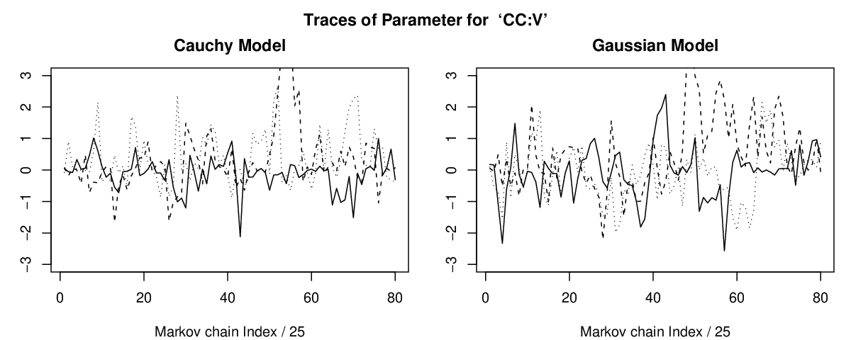
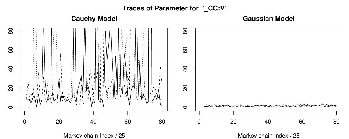
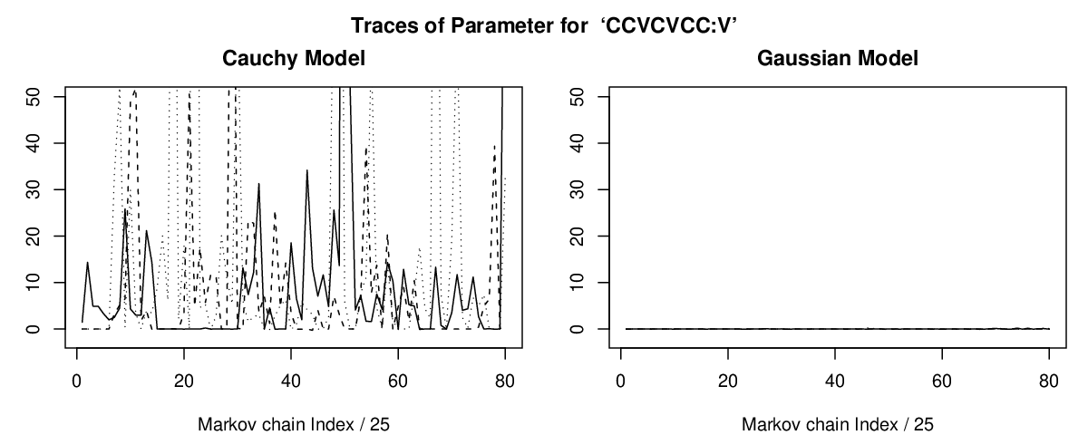
We also looked at the traces of some compressed parameters, as shown in Figure 13. The three compressed parameters shown all contain only a single . The plots on the top are for the for “CC:V”, used for predicting whether the next character is a vowel given the preceding two characters are consonants; the plots in the middle are for “__CC:V”, where “__” denotes a space or special symbol; the plots on the bottom are for “CCVCVCC:V”, which had the largest median among all compressed parameters in the Cauchy model, as shown by Figure 12. The regression coefficient for “CC:V” should be close to by our common sense, since two consonants can be followed by any of three types of characters. We can very commonly see “CCV”, such as “the”, and “CC__”, such as “with__”, and not uncommonly see “CCC”, such as “technique”,“world”, etc. The Markov chain trace of this with a Cauchy prior moves in a smaller region around than with a Gaussian prior. But if we look back one more character, things are different. The regression coefficient for “__CC:V” is fairly large, which is not surprising. The two consonants in “__CC:V” stand for two letters in the beginning of a word. We rarely see a word starting with three consonants or a word consisting of only two consonants. The posterior distribution of this for both Cauchy and Gaussian models favor positive values, but the Markov chain trace for the Cauchy model can move to much larger values than for the Gaussian model. As for the high-order pattern “CCVCVCC”, it matches words like “statistics” or “statistical”, which repeatedly appear in an article introducing a statisics department. Again, the Markov chain trace of this for the Cauchy model can move to much larger values than for Gaussian model, but sometimes it is close to , indicating that there might be two modes for its posterior distributution.
The above investigation reveals that a Cauchy model allows some useful to be much larger in absolute value than others while keeping the useless in a smaller region around than a Gaussian model. In other words, Cauchy models are more powerful in finding the information from the many possible high-order interactions than Gaussian models, due to the heavy two-sided tails of Cauchy distributions.
4 Conclusion and Discussion
In this paper, we have proposed a method to effectively reduce the number of parameters of Bayesian classification and regression models with high-order interactions, using a compressed parameter to represent the sum of all the regression coefficients for the predictor variables that have the same values for all the training cases. Working with these compressed parameters, we greatly shorten the training time with MCMC. These compressed parameters can later be split into the original parameters efficiently. We have demonstrated, theoretically and empirically, that given a data set with fixed number of cases, the number of compressed parameters will have converged before considering the highest possible order. Applying Bayesian methods to regression and classification models with high-order interactions therefore become much easier after compressing the parameters, as shown by our experiments with simulated and real data. The predictive performance will be improved by considering high-order interactions if some useful high-order interactions do exist in the data.
We have devised an efficient scheme for compressing parameters of Bayesian logistic sequence prediction models, as described in Section 3. The algorithm for sequence prediction models is efficient. The resulting groups of interaction patterns have unique expressions. We have also found similar schemes for compressing parameters of general Bayesian classification models with discrete features, though it is more difficult, see (Li 2007).
We have also empirically demonstrated that Cauchy distributions with location parameter , which have heavy two-sided tails, are more appropriate than Gaussian distributions in capturing the prior belief that most of the parameters in a large group are very close to but a few of them may be much larger in absolute value, as we may often think appropriate for the regression coefficients in certain problems.
We have implemented the compression method only for classification models in which the response and the features are both discrete. Without any difficulty, the compression method can be used in regression models in which the response is continuous but the features are discrete, for which we need only use another distribution to model the continuous response variable, for example, a Gaussian distribution. Unless one converts the continuous features into discrete values, it is not clear how to apply the method described in this paper to continuous features. However it seems possible to apply the more general idea that we need to work only with those parameters that matter in the likelihood function when training models with MCMC, probably by transforming the original parameters.
Acknowledgements
This research was supported by Natural Sciences and Engineering Research Council of Canada. Radford Neal holds a Canada Research Chair in Statistics and Machine Learning.
References
-
Baker, J. K. (1975), “The Dragon system - an overview”, IEEE Transactions on. Acoustic Speech Signal Processing ASSP-23(1): 24-29.
-
Bell, T. C., Cleary, J. G., and Witten, I. H. (1990), Text Compression, Prentice-Hall
-
Feller, W. (1966), “An Introduction to Probability Theory and its Applications”, Volume II, New York: John Wiley
-
Li, L. (2007), Bayesian Classification and Regression with High Dimensional Features, Ph.D. Thesis, University of Toronto, available from http://math.usask.ca/longhai.
-
Neal, R. M. (2003), “Slice Sampling”, Annals of Statistics, vol. 31, p. 705-767
-
Ritchie, M. D., Hahn, L. W., Roodi, N., Bailey, L. R., Dupont,W. D., Parl,F. F., and Moore, J.H. (2001), “Multifactor-Dimensionality Reduction Reveals High-Order Interactions among Estrogen-Metabolism Genes in Sporadic Breast Cancer”, The American Journal of Human Genetics, volume 69, pages 138-147
-
Romberg, J., Choi, H. and Baraniuk, R. (2001), “Bayesian tree-structured image modeling using wavelet-domain hidden Markov models”, IEEE Transactions on image processing 10(7): 1056-1068.
-
Sun, S. (2006), “Haplotype Inference Using a Hidden Markov Model with Efficient Markov Chain Sampling”, Ph.D. Thesis, University of Toronto
-
Thisted, R. A. (1988), Elements of Statistical Computing, Chapman and Hall.