DFF 438/11/07
Semiclassical Droplet States
in Matrix Quantum Hall Effect
Andrea CAPPELLI a , Ivan D. RODRIGUEZ a,b
a Istituto Nazionale Fisica Nucleare
b Dipartimento di Fisica, Universitá di Firenze
Via G. Sansone 1, 50019 Sesto Fiorentino (FI), Italy
We derive semiclassical ground state solutions that correspond to the quantum Hall states earlier found in the Maxwell-Chern-Simons matrix theory. They realize the Jain composite-fermion construction and their density is piecewise constant as that of phenomenological wave functions. These results support the matrix theory as a possible effective theory of the fractional Hall effect. A crucial role is played by the constraint limiting the degeneracy of matrix states: we find its explicit gauge invariant form and clarify its physical interpretation.
1 Introduction
In this paper we continue the study of noncommutative and matrix gauge theories [1][2][3] that can be used as effective non-relativistic theories** * We refer to [15] for an introduction to noncommutative theories of the quantum Hall effect. [4][5] of the fractional Hall effect [6]. The original Susskind proposal was based on the noncommutative Chern-Simons theory [7]: it developed in the Polychronakos Chern-Simons matrix model [8], that was analysed by several authors [9] [10] [11] [12] [13] [14] [15][16]. This model is a gauge theory in one dimension (i.e. time) with Chern-Simons kinetic term; it involves two Hermitean matrix coordinates, , that are noncommuting, , where is a constant “background charge” and is the identity matrix. In the semiclassical limit [7], the matrix model describes two-dimensional incompressible fluids in strong magnetic field with Laughlin’s values of the filling fraction, , where is integer quantized [17].
At the full quantum level, some problems were found in matching the matrix model to the physics of the fractional Hall effect: one point was that the theory reduced to the eigenvalues, , , of , does not really describe electrons in the lowest Landau level with coordinates ; owing to matrix noncommutativity, the Laughlin wave function is deformed at short distances [11][15]. Another issue was that this model cannot easily describe the general Hall states with Jain’s filling fractions: , [18].
In our earlier paper [19], we showed that these problems can be overcome by upgrading the Chern-Simons model to the Maxwell-Chern-Simons matrix theory. This includes an additional kinetic term quadratic in time derivatives and the potential, , with the coupling that controls matrix noncommutativity. All terms in the action are determined by the gauge principle because they can be obtained by dimensional reduction of Maxwell-Chern-Simons gauge theory, as discussed in the literature of D0-branes in string theory [3].
The Maxwell-Chern-Simons matrix theory reduces to the earlier Chern-Simons model for large values of (with finite ). However, in the different limit (with finite ), corresponding to , it does provide a sensible physical description of the fractional Hall effect: after reduction to eigenvalues, one finds electrons in Landau levels interacting with a two-dimensional potential of Calogero type, (see section 2.2). For general , the additional coupling in the theory allows one to interpolate between matrix () and electron () dynamics.
Furthermore, the theory is exactly solvable at [19]: it was found to describe a matrix extension of the Landau levels, where the gauge-invariant many-body states are given by matrix generalizations of Slater determinants. Although the degeneracy of matrix states grows exponentially with energy, it was possible to control it by introducing suitable projections in the theory. We showed that the constraint , , projects the theory to the “lowest matrix Landau levels”, with ; the -th reduced theory naturally possesses non-degenerate homogeneous ground states with filling fractions of the Jain series, [19] (see section 2). Indeed, the solutions of the gauge invariance conditions and of the constraint give raise to a rather surprising structure of ground states that corresponds to the Jain composite-fermion construction of ansatz wave functions [18].
These states exactly match the phenomenological Jain wave functions under matrix diagonalization, that is formally achieved at . Therefore, we conjectured that these matrix ground states have smooth deformations for into the physical states, namely that no phase transitions are found for when the system is at the specific densities [19].
A number of problems remained to be further investigated:
- •
Understand the matrix Jain states, e.g. compute their densities and observables quantities.
- •
Understand the projections in more physical terms.
- •
Study the phase diagram of the theory for at the relevant densities.
In the present paper, after reminding earlier results [19] (section 2), we find the gauge invariant form of the projection and its semiclassical physical meaning in terms of single-particle occupancy (section 3). Next, we study the matrix Jain states in the semiclassical approximation, by analytically solving the classical equations of motion, further constrained by the Gauss law and the semiclassical version of the condition (section 4). The ground states are found to be two-step droplets of incompressible fluid with piecewise constant density; this is the same density shape of the phenomenological Jain states before projection to the lowest Landau level [18] (where the density of incompressible fluids becomes strictly constant).
The fact that the matrix Jain states at already have the expected droplet density of physical states, supports our earlier claim that these ground states could remain stable while varying [19]. Other ground states corresponding to generalized Jain constructions with different filling fraction, although possible in the theory, are found not to possess piecewise constant density. We argue that the modulated density shape is a signal of ground-state instability at finite values, since the corresponding phenomenological Jain states () are known to be unstable [18]. We complete our study of semiclassical solutions by describing the quasi-holes excitations above the matrix Jain states. Finally, in the conclusion we briefly discuss the ways to study the Maxwell-Chern-Simons matrix theory for .
2 Jain states in Maxwell-Chern-Simons matrix gauge theory
2.1 Lagrangian and Hamiltonian
In this section we recall the matrix theory of quantum Hall states proposed in [19] and the derivation of ground states that are matrix analogs of the Jain composite-fermion states. The theory involves three time-dependent Hermitean matrices, , and , and an auxiliary complex vector . The Lagrangian contains a Maxwell-Chern-Simons kinetic term, a uniform “charge background” and the “boundary term” of ref.[8]:
| (2.1) | |||||
The covariant derivatives are: and . Under the gauge transformations: , , and , the action changes by a total derivative, such that invariance under large gauge transformations requires the quantization, [17]. Hereafter we set and measure dimensionful constants accordingly.
The variation of w.r.t. the non-dynamical field gives the Gauss-law constraint; its expression in term of coordinates and conjugate momenta , , reads:
| (2.2) |
The trace of fixes the norm of the auxiliary vector ,
| (2.3) |
We note that has trivial dynamics, , and it is necessary to represent the Gauss law on finite-dimensional matrices that have traceless commutators [8]. In a gauge in which all components vanish but the last one, the term in (2.2) becomes the “traceless identity”, , .
In gauge-invariant quantization, all matrix degrees of freedom are quantized and the Gauss law is imposed on states: generates gauge transformations of and , and implies that physical states are singlets subjected to the additional condition (2.3) fixing the total number of components equal to . The Hamiltonian can be written:
| (2.4) |
after introducing the variable,
| (2.5) |
and its adjoint , involving the magnetic length, . These quantities obey the commutation relations of independent harmonic oscillators:
| (2.6) |
Therefore, for the Hamiltonian describes Landau levels populated by two-dimensional “particles” with phase-space coordinates, , , . Degenerate angular momentum excitations are described by an independent set of oscillators:
| (2.7) |
| (2.8) |
that commute with . The total angular momentum of the particles is
| (2.9) |
The - particle states are further constrained by the Gauss law (2.2): as we shall see later, this enforces a kind of generalized exclusion statistics. It is convenient to introduce the complex matrices,
| (2.10) |
and use the bar for denoting the Hermitean conjugate of classical matrices, keeping the dagger for the quantum adjoint. Hereafter we set the magnetic length to one, i.e. .
For states with constant density†† † See section 4 for the definition of density in matrix theories., the angular momentum measures the extension of the “droplet of fluid”, such that we can relate it to the semiclassical filling fraction by the formula,
| (2.11) |
In a physical system of finite size, one can control the density of the droplet by adding a confining potential to the Hamiltonian:
| (2.12) |
The strength is of order such that the structure of Landau levels is not destroyed by putting particles per level. The higher order terms also commute with the Hamiltonian: one can show that their eigenvalues on constant-density states are very large for fillings and thus they can be used to simulate finite-box boundary conditions [19].

In Figure (1) we illustrate the phase diagram of the Maxwell-Chern-Simons matrix theory as a function of the parameters and . The analysis of [19] found the properties of the theory on the axes and . For , the theory is exactly solvable and possess a set of ground states that are in one-to-one relation with the Laughlin and Jain ground states with filling fractions . These states are selected by the value of and by adjusting the density via the parameters of the confining potential (2.12); furthermore, they are unique non-degenerate states obeying the conditions that projects out degeneracies specific of matrix states, as it will be explained momentarily.
The limit at (and finite) in the Hamiltonian (2.4) corresponds to vanishing kinetic term, i.e. to the constraints of lowest Landau level [20]. In this limit, the Gauss law (2.2) reduces to:
| (2.13) |
and it uniquely fixes the noncommutativity of matrices. The potential term in (2.4) becomes a constant for all physical states and the theory reduces to the Chern-Simons matrix model [8] with trivial dynamics, [19].
For ( finite), the theory describes ordinary electrons with coordinates given by the complex eigenvalues , , of , interacting with the two-dimensional Calogero potential.
2.2 limit and electron theory
For large values, the potential term in (2.4), , restricts the configuration space of complex matrices to those commuting with their conjugate, the so-called “normal” matrices [21]. Therefore, can be made diagonal by unitary (gauge) transformation and the theory completely reduces to the eigenvalues, that are interpreted as electron coordinates. Any complex matrix can be written [22] as, , in terms of a unitary matrix (the gauge degrees of freedom), a diagonal matrix (the eigenvalues) and a upper triangular complex matrix (additional d.o.f.). Therefore, the gauge-invariant degrees of freedom different from the eigenvalues contained in the matrix are suppressed for .
We can thus take the diagonal gauge for and decompose the momenta in diagonal and off-diagonal matrices, respectively called and :
| (2.14) |
In this gauge, the Gauss law (2.2) can be solved at the classical level and it determines the off-diagonal momenta,
| (2.15) |
Upon inserting them into the Hamiltonian (2.4), the diagonal and off-diagonal components decouple and one obtains,
| (2.16) |
The quantization can be done on the remaining independent variables, which are the complex eigenvalues and their conjugate momenta [23]. Therefore, the theory reduced to the eigenvalues corresponds to the ordinary Landau problem of electrons plus an induced two-dimensional Calogero interaction. The measure of integration on matrices (2.18) also reduces to that of ordinary electrons after incorporating one Vandermonde factor in the wave functions [21]. This causes a renormalization of the filling fraction from the semiclassical expression (2.11):
We conclude that the Maxwell-Chern-Simons matrix theory in the limit makes contact with the physical problem of the fractional quantum Hall effect: the only difference is that the Coulomb repulsion is replaced by the Calogero interaction . Numerical results [24][25] [18][26] indicate that quantum Hall incompressible fluid states are rather robust and do not depend on the detailed form of the repulsive potential at short distance, for large , at least for the qualitative features. The theory is not, by itself, less difficult than the ab-initio quantum Hall problem: the gap is non-perturbative and there are no small parameters. The advantage of embedding the problem into the matrix theory is that of making contact with the solvable limit.
2.3 Matrix Jain states at
The wave functions of the Maxwell-Chern-Simons theory take the form,
| (2.17) |
and their integration measure reads:
| (2.18) |
At , the energy and momentum eigenstates are obtained by applying powers of the and operators (2.5,2.7) to the empty ground state (as in ordinary Landau levels), leading to:
| (2.19) |
The wavefunction is a homogeneous polynomial of and , that can be treated as -number matrices because they commute among themselves. The energy and momentum of the state are expressed in terms of the eigenvalues of and , and respectively, that count the total number of matrices and in .
In the lowest Landau level, the wave function obeys , , thus the polynomial part does not contain any : it is a analytic function of the variables, equal to the . The physical states obeying the Gauss law are singlets that contain any number of and copies of the vector (owing to (2.3)). The solutions for are given by [10]:
| (2.20) |
where is the completely antisymmetric tensor and any ordered set of integers. Solutions for are obtained by multiplying terms (2.20), leading to the expressions, . The ground state in the confining potential is given by the closest packing that has the lowest angular momentum, i.e. lowest degree in :
| (2.21) |
If we diagonalize the complex matrix by similarity transformation: , , , the dependence on and factorizes and the powers of eigenvalues make up the Vandermonde determinant , as follows:
| (2.22) |
The central piece is indeed the Laughlin wave function [24], upon interpreting the eigenvalues as electron coordinates [10] [11]. The value of the filling fraction (2.11) is:
| (2.23) |
by keeping into account the extra Vandermonde coming from the integration measure.
Eq.(2.22) is the most interesting result obtained in the noncommutative approach and the Chern-Simons matrix model [8][10]: that of deriving the Laughlin wave function from gauge invariance in a matrix theory with background charge . Furthermore, Susskind’s semiclassical analysis [7] showed that, in the limit , this matrix state describes an incompressible fluid in high magnetic fields with density, , and classical filling fraction in agreement with the earlier identification.
The analog of the Laughlin quasi-holes are realized by shifting the occupation numbers of matrices, e.g. by the state in (2.20) with . This has and thus a finite gap . On the other hand, the quasi-particle excitations cannot be realized in the Chern-Simons matrix model [8]. In general, states with higher density do not exist in this theory, because they would need to populate higher Landau levels that are absent.
Further difficulties in matching the Chern-Simons matrix model to the Laughlin physics at the quantized level were discussed in Refs. [11][15][13]: since the matrices are noncommuting (cf. (2.13)), the theory is not well suited for the description of electron degrees of freedom. The reduction [15] to eigenvalues , interpreted as electron coordinates, shows that the measure of integration (2.18) does not become that of the Landau levels and the Laughlin state (2.22) gets deformed at short distance. These findings should be contrasted with the results in section 2.2 for Maxwell-Chern-Simons matrix theory, that possesses a well-definite physical limit at (although difficult to solve).
The states (2.20) can be represented graphically as “bushes”, as shown in Fig.(2a). The matrices (i.e. ) are depicted as oriented segments with indices at their ends and index summation amounts to joining segments into lines, as customary in gauge theories. The lines are the “stems” of the bush ending with one , represented by an open dot, and the epsilon tensor is the N-vertex located at the root of the bush. Bushes have N stems of different lengths: . The position of one on the -th stem, , is called the “height” on the stem.

The solutions of the Gauss law (2.2) for states in higher Landau levels are polynomials involving both and matrices: given that they transform in the same way under the gauge group, these polynomials can be represented by bushes whose stems are arbitrary words of and , as shown in Fig.(2b, 2c), where is represented by a bold segment. Since two stems cannot be equal, one obtains a kind of Fermi sea of “one-particle states” corresponding to the strands. However, there are additional degeneracies with respect to an ordinary fermionic system, because in each stem all possible words of and of given length yield independent states (for large ), owing to matrix noncommutativity, as seen in fig.2(b) and 2(c).
The complete filling of all the available degenerate states clearly gives very dense and inhomogeneous fluids that are incompatible with the physics of the quantum Hall effect. Moreover, the matrix degeneracies lead to a density of states in the theory that grows exponentially with the energy. This is a characteristic of string theories that is not suitable for the Hall effect [3]. Of course, for the potential restricts the matrix noncommutativity and reduces the degeneracy: at , this is not present and the theory can describe a physical electron system, as is clear from the discussion of section 2.2.
Given that the theory is very difficult to solve, in ref. [19] we introduced a set of projections that limit the matrix degeneracy at and are explicitly solvable. These projections are expressed by the following constraints on the wave function,
| (2.24) |
for a given value of . The case is the lowest Landau level discussed before with no dependence, while taking successive values gradually allow larger multiplicities and thus matrix degeneracies. Note that in equation (2.24), each matrix component is raised to the -th power, without index summation: the condition is nevertheless gauge invariant and it admits an equivalent manifestly invariant form that is discussed in section 3.
The results of ref.[19] were rather interesting: not only the projections (2.24) allow homogeneous ground states suitable for describing quantum Hall fluids, but also they precisely occur in the Jain pattern of filling fractions, , and their derivation repeats step-by step the Jain “composite fermion” construction [18].
Let us recall the main points of the analysis of [19]. Consider first the projection (2.24) for : the solutions are polynomials that are at most linear in each component . Let us imagine that one or more matrices are present at points on the bush as in Fig.(2). The differential operator (2.24) acts by sequentially erasing pairs of bold lines on the bush, each time detaching two strands and leaving four free extrema with indices fixed to either or , with no summation on them. For example, when acting on a pair of located on the same stem, it yields a non-vanishing result: this limits the bushes to have one per stem at most. The conditions can be satisfied if cancellations occur for pairs of on different stems, as it follows:
| (2.25) |
This expression vanishes for due to the antisymmetry of the epsilon tensor. The general solution of (2.24) is given by bushes involving one per stem at most (max N matrices in total), with all of them located at the same height on the stems [19]. In formulas:
| (2.26) | |||||
If the matrices were diagonal, these states would be Slater determinants of ordinary Landau levels. The matrix states have further degeneracies by commuting pairs: however, commutations are almost impossible in the the solution (2.26) of the constraint, were it not for the dependence. This shows how the projection works in reducing matrix degeneracies.
The ground state in the theory with finite-box conditions corresponds to homogeneous filling all the allowed states in the first and second Landau levels with “gauge invariant particles” each. It reads:
| (2.27) |
with angular momentum . This state is non-degenerate due to the vanishing of the parameter in (2.26). It has filling fraction , assuming homogeneity of its density‡‡ ‡ This will be shown in section 4..
The ground states for are products of bushes: they obey the constraint provided that the two derivatives always vanish when distributed over the bushes. Given one bush of type (2.27), obeying , one can form the state,
| (2.28) |
where the other bushes satisfy and actually are Laughlin’s one (2.20). The angular momentum value for this state corresponds to the filling fraction (cf (2.11)).
We thus find the important result that the projected Maxwell-Chern-Simons theory possesses non-degenerate ground states that are the matrix analogues of the Jain states obtained by composite-fermion transformation at , i.e. . The matrix states (2.28,2.27) would actually be exactly equal to Jain’s wave functions, if the matrices were diagonal: the dependence would factorize and the matrix states reduce to the Slater determinants of Jain’s wave functions (before their projection to the lowest Landau level) [18][26].
The correspondence extends to the whole Jain series: the other non-degenerate ground states, corresponding to , are respectively obtained in the theories with projections. They read:
| (2.29) |
where,
| (2.30) |
Note that in the theory, the lower density states that were non-degenerate in the theories, , become degenerate; actually, when the boundary potential is tuned for letting (2.30) to be the ground state, the former states become excited states. In conclusion, in ref.[19] we found that the ground states of the properly projected Maxwell-Chern-Simons matrix theory reproduce the Jain pattern of the composite fermion construction [18]; the matrix states are non-degenerate for specific values of the density that are controlled by the boundary potential.
These results indicate that the Jain composite fermions have some relations with the D0-brane degrees of freedom and their underlying gauge invariance. Both of them have been described as dipoles: according to Jain [18] and Haldane-Pasquier [27], the composite fermion can be considered as the bound state of an electron and a hole (a vortex in the electron fluid). On the other side, matrix gauge theories, and the equivalent noncommutative theories [3], describe D0 branes that are point-like dipoles in the low-energy limit of string theory. Although further relations between these two dipole pictures remain to be found, in this paper we shall find further evidences that the matrix ground states describe semiclassical incompressible fluids with some of the properties of Hall states.
2.4 Generalized Jain’s hierarchical states
In the projected theories with , there are other solutions of the Gauss law for besides the Jain states (2.29). These are obtained by combining products of any solution (2.30), as follows:
| (2.31) |
In this equation, we also wrote the associated filling fractions using Eq.(2.11), i.e. assuming homogeneous densities, and the condition that they satisfy. The Jain mapping to a single set of effective Landau levels does not hold for these generalized states (having more than one ). Actually, analogous generalized states were considered by Jain in his composite-fermion theory [18], but were discarded due to their instability (small or vanishing numerical gap).
Let us compare the generalized (2.31) and standard (2.29) Jain states at fixed values of the background (keeping in mind that the physical values are ). The energy of the generalized states is additive in the , , blocks and reads:
| (2.32) |
The analysis of some examples shows that these additional solutions have in general higher energies for the same filling or are more compact for the same energy than the standard Jain states (2.29) (see Table 1). States of higher energies are clearly irrelevant at low temperatures; higher-density states strongly deviate from the semiclassical incompressible fluid value for background , that is specific of the Laughlin factors [7]. The analysis of the corresponding semiclassical states in section 4 will show that most of these states are not incompressible fluids (density not piecewise constant).
3 Properties of the projection
In this section we discuss the physical meaning of the projection:
| (3.1) |
that limits the degeneracy of matrix quantum states at . Although the operator is not gauge invariant, its kernel restricted to gauge invariant states yields a gauge invariant condition§§ § A formal proof of this statement is given in Appendix A, as explicitly seen in section 2. Therefore, there should exist a manifestly gauge invariant expression for this condition, that is found in this section.
A simple example is useful to clarify the following discussion. In a two dimensional quantum mechanical problem with rotation invariance ( global symmetry), we consider the condition:
| (3.2) |
where is a reduced (polynomial) wave function. The condition is not invariant but its kernel acting on rotation invariant functions does: indeed, it limits the order of the polynomial to . This example suggests two remarks:
- •
The condition (3.2) can have many different forms, that correspond to points on its orbit in the “gauge” group: for example, an equivalent form is , corresponding to a rotation. All these conditions are equally satisfied.
- •
A manifestly gauge-invariant expression can be obtained by integrating over the gauge orbit, as follows:
(3.3)
However, this vanish for odd: the average looses information because the operator is not positive definite. Clearly, it can be made positive (and gauge invariant) by contracting with another gauge-dependent term to obtain powers of the dilatation operator .
We are now going to follow analogous steps for the condition . First we find an equivalent, more general form. Consider an infinitesimal gauge transformation : the Hermitean matrix can be expressed by the matrices with a single non-vanishing component, , in symmetric or antisymmetric combinations, or . Upon performing the gauge transformation, the constraint (2.24), , acquires an additional term that should also vanish on the wave functions obeying, :
| (3.4) |
We now analyse the various cases:
- •
I. If and or , we obtain the conditions,
- •
II. If , we obtain,
Note that each term in the linear combination of case II.3 independently vanishes by case I.
These conditions can be summarized as follows:
| (3.5) |
They are more general than the original expression (2.24) for , corresponding to or . Of course, iteration to of the gauge transformation produce further identities: these involve linear combinations of terms that are not particularly useful; for example, one such condition is: .
The analysis is necessary to obtain the generalized constraint for : the expression is similarly, , and its further transformation yields,
This expression contains the constraint analogous to (3.5):
| (3.6) |
together with other relations involving linear combinations of cubic terms.
Following the example, we can now transform the new expressions (3.5) into positive definite operators. We recall that the lowest Landau level condition corresponds to the vanishing of the total energy, that is a sum of positive terms:
| (3.7) |
We can construct the following positive definite expressions:
| (3.8) | |||||
| (3.9) |
whose vanishing is equivalent to the conditions (3.5). These quantities are not yet gauge invariant but are convenient for the physical interpretation. We introduce the (gauge variant) energy operators for one-particle matrix states, that are summed over matrix indices of one row or column of , or , respectively:
| (3.10) |
Using these energy operators, we can rewrite (3.8,3.9) as follows:
| (3.11) |
In this form, the constraints admit the following physical interpretation: there is a gauge choice in which the allowed states contains at most one “particle” in the second Landau level (energy equal to one) for indices belonging to each row and column.
The constraint for (2.24) similarly becomes:
| (3.12) |
This requires that there at most 2 particles in the second Landau level or a single particle in the third level for any set of indices in a row or column. The matrix labels are not gauge invariant, then these occupancies are only verified in specific gauges; nevertheless, the present form of the constraints can be implemented in the semiclassical limit on expectation values, , as explained in section 4.
Next, we obtain the gauge-invariant form of the constraint by averaging over the gauge group. We define:
| (3.13) |
where is the invariant Haar measure [28]. The integrand is positive definite for any value, because it can be thought of as the norm of a vector: , where is a rotated unit vector. Therefore, we do not loose any information by performing the group average.
Group integrals of products of matrices can be found e.g. in ref.[28]: their results can be described as follows. Representing the unitary matrices with upper and lower indices, , , the result of integrating pairs is a combination of delta functions relating the upper indices among themselves times other deltas connecting the lower indices. The simplest integral is:
In the general case of pairs, the pairings of upper (lower) indices by delta functions follow patterns given by the permutation of elements, with specific weight for each conjugacy class of permutations [28]. For , one finds:
In the case of the constraint (3.9), all the upper indices are simultaneously taking the same value ; thus, the different delta-function pairings of upper indices take the same unit value. As a result, the pairings of lower indices get averaged over, and reduce to a plain sum over all pair permutations:
| (3.14) |
Upon commuting the operators to bring summed indices close each other, we finally find the manifestly gauge-invariant form of the constraint (disregarding the normalization):
| (3.15) |
The same expression is also obtained by group averaging the other operator in (3.8). One can check that the action of the gauge-invariant constraint on bush wave functions (cf. section 2) is completely equivalent to that of the gauge-variant condition [19].
The gauge invariant form of the constraint can be similarly obtained by group averaging (3.6), leading to:
| (3.16) |
The form of this expression corresponding to (3.15) is not particularly illuminating. The gauge-invariant expression (3.16) straightforwardly generalizes to higher values.
In conclusion, in this section we have found equivalent forms of the projections of matrix states: the first expression (3.11,3.12) in terms of occupation numbers is useful for the semiclassical limit considered in the next section; the second expression (3.15,3.16) is manifestly gauge invariant. In the latter form, the constraint can be added to the Hamiltonian with a large positive coupling constant to realize a softer form of projection, where matrix states violating the constraint are now allowed but possess very high energy. For example, the quasi-particles excitations over the Jain ground states would be possible, while they are absent in the -projected theory, as explained in section 3. A detailed analysis of this issue is postponed to a following publication.
4 Droplet ground state solutions
In this section we study the Maxwell-Chern-Simons theory in the semiclassical limit: we solve the classical equation of motion including the quantum constraints, first for the ground states and then for the quasi-hole excited states. We shall find the semiclassical states that correspond to the quantum states with homogeneous filling and composite-fermion structure of section 2 [19]. The motivations for this semiclassical analysis are twofold: on one side, previous experience [8][3][12][13] [16] with noncommutative field theory has shown that the classical fluid dynamics incorporates some properties of the full quantum theory. From another side, it is know that the Laughlin states in the quantum Hall effect are incompressible fluids that become semiclassical in the thermodynamic limit [29][30]. The semiclassical ground states we find in this section are also incompressible fluids which, we believe, may give rather accurate descriptions of the quantum matrix states for large values [21].
Let us start by writing the classical equations of motion: the Hamiltonian of the Maxwell-Chern-Simons theory at can be written as follows:
| (4.1) | |||||
We set , , and included the Gauss law constraint via the Hermitean Lagrange multiplier . The projection analyzed in section 3 is enforced by adding two other Lagrange multipliers times the energies, , , of single-particle states with matrix indices summed over rows or columns. We replace the nonlinear constraints (3.11,3.12) with linear expressions involving the parameters taking the allowed values of . Since the constraints are not gauge invariant, we shall assume that we work in a gauge where they take integer values. The gauge-invariant form of the constraint (3.15) found at the end of sections 3 is also not convenient because it would lead to non-linear equations of motion that cannot be solved analytically. For the same reason, we limit the confining potential (2.12) to the quadratic term: later we shall see how to avoid ground state degeneracies that may arise with this potential.
We vary the Hamiltonian with respect to , canonically equivalent to the original , and obtain the equations:
| (4.2) | |||||
| (4.3) | |||||
| (4.4) | |||||
| (4.5) | |||||
| (4.6) |
We first discuss ground state solutions corresponding to .
4.1 Laughlin ground states
We can gain some intuition on the matrix equations (4.2,4.3,4.4,4.5) by recalling the solutions of the Chern-Simons matrix model [8], corresponding to the lowest Landau level in our theory. In the case , we have and the ground state equations reduce to:
| (4.7) |
These are the commutation relations of a truncated quantum harmonic oscillator, with playing the role of Hamiltonian. We can diagonalize it by gauge choice and write standard oscillator matrices in the “energy” basis, [8]:
| (4.8) |
In matrix form for :
| (4.9) |
The solution is characterized by the angular momentum, and by vanishing energy.
A good definition of the density of semiclassical fluids in matrix models [8] is given in terms of the gauge invariant eigenvalues of ,
| (4.10) |
In the limit , this becomes a piecewise continuous function that describes two-dimensional rotation-invariant distributions (). A discrete approximation is:
| (4.11) |
involving the Kronecker delta and the ordered set of distinct eigenvalues, , , with multiplicities .
In Polychronakos’ solution of the Chern-Simons matrix model (4.8), the matrix is already diagonal,
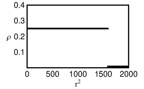
| (4.12) |
Its density (Fig. 3) is constant and describes a circular droplet of fluid with Laughlin filling fraction [7]:
| (4.13) |
Note that an ordering ambiguity in the definition of was resolved by matching to the angular momentum spectrum. As said before, there is a shift in the filling fraction in quantum theory due to a contribution from the integration measure, ; thus, should be even for describing electrons.
4.2 Jain ground states
As we showed in section 2.3, the Maxwell Chern-Simons theory contains Jain-like ground states (2.29), that involve higher Landau levels (). Their filling fractions can be written as in composite fermion construction [18],
| (4.14) |
and their energy and angular momentum values are recalled in Table 1. We first note that these states are characterized by energies and angular momentum , thus implying that the matrix must have elements of and be much smaller than . Indeed, the constraints, , limits the squares of matrix elements summed over each row or column to take at most the total value . Were it not for this constraint, the matrices could be rescaled in the ground state equations (4.2,4.3,4.4) to eliminate the dependence, leading to solutions with at least.
We now describe the solution of the ground state equations of motion in the projected theory ( in (4.5)). Under some minor hypotheses, we find a single solution corresponding to the unique quantum state with (2.28) [19]. Working in analogy with the Laughlin case (4.9), we shall try a distribution of eigenvalues leading to a piecewise constant density. We can consider the gauge in which is diagonal, , and assume that has a single non-vanishing component, i.e. the last one, as in (4.9), such that the term, , is also diagonal. The equation for (4.3),
| (4.15) |
requires that is a raising operator, i.e. non vanishing on a single diagonal, ; moreover, the Gauss law (4.4) requires, , apart from corrections due to . Therefore, should be non-vanishing on the first diagonal:
| (4.16) |
Eq. (4.15) implies evenly spaced eigenvalues, , and leaves the components undetermined. The equation (4.2) for reads:
| (4.17) |
that can always be solved for . The constraints, , imply that has one non-vanishing element per row and column, at most, equal to one. If it had exactly one element per row and column, it would be the representation of a permutation, . Therefore, we can write:
| (4.18) |
We now consider the Gauss law (4.4): all terms in this equation are diagonal matrices, leading to a system of scalar equations for the matrix elements . Note that both matrices and are diagonal and thus their elements are positive integers in the semiclassical theory: . After introducing,
| (4.19) |
we obtain the system:
| (4.20) |
The solution can be found by thinking to the expected shape of the droplet. The quantum state (2.28) is made of generalized Slater determinants with homogeneous filling of ‘‘one-particle’’ states¶¶ ¶ This Fock-space analogy is meaningful for diagonal matrices, and may not be correct in general: its limitations will be discussed in section 4.3.. Each one-particle state is expected to give a constant contribution to the density of the droplet: there are Laughlin terms and one term with “particles” in the second Landau levels spanning half of the angular momentum range, as confirmed by the quantum numbers, and . The contribution are additive in terms of angular momentum eigenvalues, (the contribution of is subdominant for ). Therefore, we expect, , for one half of the range, say , and for the other half. Moreover, should be continuous at in order to obey the corresponding equation with . We take:
| (4.21) |
The solution for is found by inspection: it has non-vanishing elements equal to one on the diagonal of the lower half sector.
Summarizing, the ansatz semiclassical ground state solution for is given by ( even):
| (4.22) |
In matrix form for , it reads:
| (4.23) |
This solution has same energy of the quantum state (2.28) and same angular momentum to leading order (cf. Table 1). The matrix contains off-diagonal terms from the mixed products: however, these give subdominant corrections to the eigenvalues as is clear in a simple two-by-two matrix example. Thus, , confirming the earlier identification of droplet shape with angular momentum spectrum.


In Fig.4(a), the density (4.11) of the droplet of fluid is plotted by computing the exact spectrum for : up to finite- fluctuations, this is a two-step constant density as anticipated. We recall that the same droplet shape is found for the Jain phenomenological states before their projection to the lowest Landau level [18]; the density becomes constant only after projection∥∥ ∥ The lowest-level projection in the matrix theory cannot be done at present, lacking an understanding of the regime: at , it would give a trivial result because the Laughlin state is the unique lowest-level ground state for any value..
In ref.[19], we argued that the matrix ground states at match one-to-one the phenomenological Jain states that are good ansatz in the physical limit : the two sets of states become identical in the limit of both diagonal, that can be formally reached at . To establish a relation at the quantum level, we would need to consider the evolution of the matrix ground states as the coupling is varied in between, , and to check that the gap never vanishes, i.e. that there are no phase transitions in plane (cf. Fig.1) separating the and regions at these density (i.e. total angular momentum) values [19]. While this behaviour remains to be proved, it is supported by the result that the matrix () and phenomenological () states have similar densities of incompressible fluids.
We also note that the solution (4.22) could also be obtained in the lowest-level theory (Chern-Simons matrix model) by replacing the matrix with different “boundary” auxiliary fields , . This multi-boundary generalization of Polychronakos’ model has been considered in ref.[9]: it naturally describes multicomponent droplets, i.e. for boundary fields. However, the description of Jain states is rather unnatural, because the number of auxiliary fields is macroscopic and should be adjusted for each Jain state; moreover, this theory does not admit the physical limit of commuting matrices.
The solution (4.22) can be easily generalized for the theory with projection , possessing a Jain ground state with : this is found at the specific density that is reached by tuning the boundary potential. The constraint now allows the components (4.18) to take values ; we assume again a single non-vanishing element per row and column, eq. (4.18), otherwise the commutator, , would have off-diagonal terms that cannot be matched in the Gauss law equation (4.4). Therefore, the equations (4.20) are unchanged. Let us recall that the quantum solution contains Laughlin terms and the piece that puts three particles in the same angular momentum state, ranging from zero to . Thus, the ansatz contains eigenvalues spaced by for of the droplet and by for of it. The matrix that solves the Gauss law (4.20) involves elements on a diagonal extending for of the matrix ( should be a multiple of ). In conclusion:
| (4.24) |
In matrix form for :
The droplet shape plotted in Fig.4(b) has again two steps, up to local fluctuations that vanish for .
The ansatz solution with in the theory again involves a matrix with two-speed spectrum and a matrix with elements , on the diagonal extending over of the matrix ( multiple of ):
| (4.39) |
In matrix form for :
The density for and is plotted in Fig.4(c).
4.3 Correspondence of semiclassical and quantum states
Here we provide a simple argument to support the identification of the semiclassical solutions with the quantum states of section 2. Consider first the correspondence for the Laughlin states, (2.21) and (4.8). We choose the gauge in which the expectation values of matrix elements on the quantum state take the classical values (4.8) found in the previous section, up to subleading corrections for . Let us rewrite the wave function in terms of these non-vanishing terms only**** ** Although this expansion should hold for , we write the case for simplicity; the expression for general can be easily inferred.:
| (4.58) | |||||
This “semiclassical wave function” describes “particles” with matrix indices, , in angular momentum states that precisely match the occupation numbers given by the classical solution (4.12), equal to , respectively. This is a self-consistent argument for the correspondence of states: in the semiclassical limit, the quantum states match the semiclassical solutions for the leading occupation numbers.
A similar relation holds for the Jain states. For , the quantum wave function is (2.28); we evaluate it on the semiclassical non-vanishing values (4.22), given explicitly for :
| (4.59) | |||||
The “one-particle” occupancies of both energy and angular momentum states given by the wave function again match the expectation values of the corresponding number operators, and , of the classical solution. The correspondence extends to the other states that have spectrum of occupancies given by (4.24,4.39). This argument support our belief that the large limit of the matrix theory is semiclassical for the incompressible fluid ground states (piecewise constant density) and their small excitations.
4.4 Generalized Jain states
In the analysis of [19], we found other quantum solutions to the constraint , for , besides Jain composite fermion wave functions. They were recalled in section 2.4, eq. (2.31) and summarized in Table 1: these are analogs of Jain’s generalized hierarchical states, made by products of two or more wave functions with higher-level fillings (). In the semiclassical analysis, we find that some of these states have corresponding solutions with piecewise constant density, while most of them do not. Besides, we find spurious ground states that are allowed by the simplistic quadratic boundary potential used in (4.1). Let us describe these solutions in turn.
4.4.1 Spurious solutions
There is a variant of the composite-fermion solution for , Eqs. (4.22,4.24), where the matrix elements take the same values, but their positions are permuted. For , this is:
| (4.60) |
The total energy and angular momentum values are the same as those of the Jain state, , (cf. Table 1). The corresponding matrix again describes a two-step droplet. In order to find the corresponding quantum state, we use the classical-quantum correspondence of the previous section. The single-particle occupation numbers of the classical solution, for e.g. , correspond to those of Laughlin factors plus the occupations , and for the components , and , respectively. These components should fit into two wave function of the type (2.26) that obey (the product wave function obeying ). The solution, rewritten in gauge invariant form, is:
| (4.61) | |||||
In this state, we recognize that some strands do not have minimal length: thus, this is an excited state for a Hamiltonian with more realistic boundary terms (2.12) realizing finite-box conditions†††† †† The quadratic potential used in (4.1) is known to yield such degeneracies ([29]).. The expectation value of the higher boundary potential on this state is actually larger than that of the Jain state (4.24) with same energy and angular momentum: this confirms our interpretation of the solution (4.60).
4.4.2 Other two-step density states
Among the generalized Jain state in Table 1, there are those made by two kinds of terms, as follows:
| (4.62) |
in the notation of Eq.(2.31). They obey, , for , and violate the composite-fermion transformation (4.14) [18]. In the droplet interpretation of classical solutions of section 4.2, we expect a density of eigenvalues equal to for half of the spectrum and for the second half. The ansatz has the two-block structure of the solution (4.22), with maximal value in agreement with the constraint.


The first non-trivial value is , i.e. in Table 1:
| (4.63) |
In matrix representation for :
The analogous state for , corresponding to , is:
| (4.73) |
and in matrix form for :
In Fig.5, we plot the density for these generalized Jain states: these are droplets with two-step constant density similar to that of composite-fermion states. At present, we do not have strong arguments to dispose of these additional states: this issue will be further discussed in the conclusion.
4.4.3 States with many-step density
Other generalized matrix Jain states (2.31) in Table 1, for , , are made by the product of three or more different terms. The simplest one for is with energy and angular momentum . Within the droplet interpretation of classical solutions discussed before, we seek for a three-step solution ( multiple of ),
However, there is no simple solution with entries , that fulfills the Gauss law equation for the same energy and angular momentum of the quantum state. We proved this fact for an ansatz with piecewise constant density making up to steps. A four-step solution (see Fig.6) can be found with quantum numbers differing macroscopically from the quantum values, : in particular, the larger angular momentum identifies it as an excited state. Presumably, the quantum state can be better approximated by allowing a very large number of steps, leading to a modulated (or singular) density profile in the large- limit. This result indicates that most of the multi-component generalized matrix quantum states found in [19] for projections , , are not semiclassical incompressible fluids.

4.5 Quasi-holes solutions
As recalled in section 2.3, the matrix theory, projected by , possess quasi-hole excitations above the Jain ground states. In this section we give the corresponding semiclassical solutions for , corresponding to deformation of the density of solution (4.22) in fig.4(a).
The classical equation of motion for and , eq. (4.2,4.3), are linear and admit a general solution for excitations:
| (4.83) |
Therefore, we should only solve the Gauss law (4.4) and the constraint (4.5).
In the two-step fluid density in fig.4(a), one can have more than one quasi-hole corresponding to punching either of the two possible fluids. A hole in the complete fluid is obtained by generalizing the quasi-hole of the Laughlin state found in ref.[8]: it is a deformation of the matrix (4.22) that describes a quasi-hole of charge situated at the origin. The matrix remains unchanged:
| (4.84) |
In matrix representation:
The corresponding density is shown in Fig.7(a).


A quasi-hole only affecting the upper layer of the fluid is shown in Fig.7(b). It is given by the solution:
| (4.94) |
with , and a positive integer. In matrix representation for and , it reads:
The displacement from the origin of the upper layer corresponds to .
It is also possible to create a circular depletion in the whole fluid, of size (charge) outside the origin at a distance (see fig.7(c)):
| (4.113) |
In matrix representation for and :
In this case, the solution of the Gauss law is obtained in terms of a two-component auxiliary field , and it holds for , namely the depletion would move back to the origin in the scaling limit .
5 Conclusion
In this paper, we have continued the study of the Maxwell-Chern-Simons matrix gauge theory as an effective theory of quantum Hall states. After providing better forms for the projection, , limiting state degeneracy, we have obtained the semiclassical ground states of the theory. They correspond to the quantum states found before [19], that reproduce the Jain composite-fermion construction of phenomenological wave functions. The density of states in the main Jain series, , has been found to be that of incompressible fluids: this confirms our expectation that the matrix states at are not too different from the physical states at . The semiclassical approximation used here is known to be valid in the large limit for both matrix [22][21] and real Hall states [29][30], in particular for incompressible fluid states.
Outside the main series of hierarchical states, other ground states are possible in the matrix theory [19], that correspond to generalized Jain constructions [18]. In Jain’s theory, these generalized states are excluded due to their low (or vanishing) gap. In the semiclassical analysis of the matrix theory, we have found that the majority of generalized states do not have piecewise constant density, i.e. are not incompressible fluids: this is an indication that they may become unstable for finite values.
The study of the phase diagram of the matrix theory is clearly necessary to make better contact between the nice results () and the physical regime (), upon varying the potential . We expect that the relevant incompressible fluid states have a smooth evolution for and we plan to include the quartic potential in the semiclassical analysis by means of a mean-field approximation.
The explicit semiclassical solutions in this paper can also be useful to study the symmetries and algebraic properties of matrix ground states. We would like:
- •
To make contact with the symmetry of the conformal field theories describing the edge excitations of Jain states [31].
- •
To find a projection of states more refined than , that could discriminate the hierarchical Jain states from the generalized (unstable) ones. Such an expectation is based on the general belief that the observed Hall states should be uniquely characterized by algebraic conditions and gauge invariance, rather than by detailed dynamics, because they are exceptionally robust and universal.
Acknowledgments
We thank F. Colomo and G. R. Zemba for interesting discussions. I. D. Rodriguez thanks the EC program Alban of Ph-D scholarships for Latin American students. This work was partially funded by the ESF programme “INSTANS: Interdisciplinary Statistical and Field Theory Approaches to Nanophysics and Low Dimensional Systems”.
Appendix A Appendix
A.1 Gauge invariance of the projection
Here is an explicit proof that the projection (cf 2.24) is a gauge invariant condition on quantum states. Consider the more general relation for :
| (A.1) |
The wave function is assumed to be gauge invariant: . The form in the r.h.s. is specific of the bush states of section 2, but this is not relevant for the argument. The matrix vanishes for because is assumed to be one solution of the constraint. In general, there are several terms in the r.h.s. with that structure, but the matrices should all vanish independently because they are multiplied by monomials that are all independent [19].
Let us now multiply by unitary matrices and sum over indices on both sides to realize a gauge transformation of the two ’s:
| (A.2) | |||||
The resulting expression of vanishes whenever does, i.e. for , because both vanish by polynomial identities that do not depend on the specific vales of the variables. Therefore, a solution of the constraint remains a solution after gauge transformation.
References
- [1] N. Seiberg and E. Witten, String theory and noncommutative geometry, JHEP 9909 (1999) 032; M. R. Douglas and N. A. Nekrasov, Noncommutative field theory, Rev. Mod. Phys. 73 (2001) 977.
- [2] G. Landi, An introduction to noncommutative spaces and their geometry, Lecture Notes in Physics m51, Springer, Berlin (1997); F. Lizzi, Noncommutative geometry in physics: A point of view, Nucl. Phys. Proc. Suppl. 104 (2002) 143.
- [3] T. Banks, W. Fischler, S. H. Shenker and L. Susskind, M theory as a matrix model: A conjecture, Phys. Rev. D 55 (1997) 5112 [hep-th/9610043]; for a review, see: W. Taylor, M(atrix) theory: Matrix quantum mechanics as a fundamental theory, Rev. Mod. Phys. 73 (2001) 419 [hep-th/0101126].
- [4] A. Lopez, E. Fradkin, Fractional Quantum Hall Effect and Chern-Simons gauge theories, Phys. Rev. B 44 (1991) 5246; Universal properties of the wave functions of fractional quantum Hall systems, Phys. Rev. Lett. 69 (1992) 2126; Fermionic Chern-Simons Field Theory for the Fractional Hall Effect, in Composite Fermions in the Quantum Hall Effect, O. Heinonen editor, World Scientific, Singapore (1998) [cond-mat/9704055].
- [5] S. Kivelson, D.-H. Lee, and S.-C. Zhang, Global phase diagram in the quantum Hall effect, Phys. Rev. B 46, 2223 (1992); S. C. Zhang, The Chern-Simons-Landau-Ginzburg theory of the fractional quantum Hall effect, Int. J. Mod. Phys. B 6 (1992) 25; G. Murthy, R. Shankar, Hamiltonian Theories of the FQHE, Rev. Mod. Phys.75 (2003) 1101.
- [6] For a review see: R. A. Prange and S. M. Girvin, The Quantum Hall Effect, Springer, Berlin (1990); S. Das Sarma and A. Pinczuk, Perspectives in Quantum Hall effects, Wiley, New York (1997).
- [7] L. Susskind, The quantum Hall fluid and non-commutative Chern Simons theory, hep-th/0101029.
- [8] A. P. Polychronakos, Quantum Hall states as matrix Chern-Simons theory, JHEP 0104 (2001) 011; Quantum Hall states on the cylinder as unitary matrix Chern-Simons theory, JHEP 0106 (2001) 070.
- [9] B. Morariu and A. P. Polychronakos, Finite noncommutative Chern-Simons with a Wilson line and the quantum Hall effect, JHEP 0107 (2001) 006.
- [10] S. Hellerman and M. Van Raamsdonk, Quantum Hall physics equals noncommutative field theory, JHEP 0110 (2001) 039.
- [11] D. Karabali and B. Sakita, Orthogonal basis for the energy eigenfunctions of the Chern-Simons matrix model, Phys. Rev. B 65 (2002) 075304; Chern-Simons matrix model: Coherent states and relation to Laughlin wavefunctions, Phys. Rev. B 64 (2001) 245316.
- [12] T. H. Hansson and A. Karlhede, Charges and Currents in the Noncommutative Chern-Simons Theory of the QHE, cond-mat/0109413; T. H. Hansson, J. Kailasvuori and A. Karlhede, Charge and Current in the Quantum Hall Matrix Model, Phys. Rev. B 68, 035327 (2003).
- [13] T. H. Hansson, J. Kailasvuori, A. Karlhede and R. von Unge, Solitons and Quasielectrons in the Quantum Hall Matrix Model, Phys. Rev. B 72, 205317 (2005).
- [14] E. Fradkin, V. Jejjala and R. G. Leigh, Non-commutative Chern-Simons for the Quantum Hall System and Duality, Nucl. Phys. B 642 (2002) 483.
- [15] A. Cappelli and M. Riccardi, Matrix model description of Laughlin Hall states, J. Stat. Mech. 0505 (2005) P001.
- [16] J. Lambert and M. B. Paranjape, Quasi-hole solutions in finite noncommutative Maxwell-Chern-Simons theory, JHEP 0705 (2007) 007
- [17] V. P. Nair and A. P. Polychronakos, On level quantization for the noncommutative Chern-Simons theory, Phys. Rev. Lett. 87 (2001) 030403.
- [18] J. K. Jain, Composite fermion approach for the fractional quantum Hall effect, Phys. Rev. Lett. 63 (1989) 199; J. K. Jain and Camilla, Int. J. Mod. Phys. B 11 (1997) 2621; for reviews see: J. K. Jain, Composite Fermions, Cambridge Univ. Press (2007), Cambridge.
- [19] A. Cappelli, I. D. Rodriguez, Jain states in a matrix theory of the quantum Hall effect, JHEP 0612 (2006) 056.
- [20] G. V. Dunne, R. Jackiw and C. A. Trugenberger, ’Topological’ (Chern-Simons) Quantum Mechanics, Phys. Rev. D 41 (1990) 661.
- [21] P. Wiegmann, A. Zabrodin, Large N expansion for normal and complex matrix ensembles, hep-th/0309253; for a review, see: A. Zabrodin Matrix Models and Growth Processes: From viscous flows to the Quantum Hall Effect, in Applications of Random Matrices in Physics, Les Houches Summer School 2004; J. Feinberg, Quantized normal matrices: Some exact results and collective field formulation, Nucl. Phys. B 705 (2005) 403; Non-Hermitean Random Matrix Theory: Summation of Planar Diagrams, the ”Single-Ring” Theorem and the Disk-Annulus Phase Transition, J.Phys. A 39 (2006) 10029.
- [22] E. Brezin, C. Itzykson, G. Parisi and J. B. Zuber, Planar Diagrams, Commun. Math. Phys. 59 (1978) 35; J. Ginibre J. Math. Phys, 6 (1965) 440; M.L. Mehta, Random Matrices and the statistical theory of energy levels, Academic Press, New York (1967).
- [23] A. P. Polychronakos, Multidimensional Calogero systems from matrix models, Phys. Lett. B 408 (1997) 117.
- [24] R. B. Laughlin, Phys. Rev. Lett. 50 (1983) 1395; Elementary Theory: the Incompressible Quantum Fluid, in R. A. Prange and S. M. Girvin, ref. [6].
- [25] F. D. M. Haldane, The hierarchy of fractional states and numerical studies, in R. A. Prange and S. M. Girvin [6].
- [26] A. Cappelli, C. Méndez, J. Simonin, G. R. Zemba, Numerical study of hierarchical quantum Hall edge states on the disk geometry, Phys. Rev. B 58 (1998) 16291.
- [27] V. Pasquier, Skyrmions in the quantum Hall effect and noncommutative solitons, Phys. Lett. B 490, 258 (2000) [hep-th/0007176]; V. Pasquier, F.D.M. Haldane, A dipole interpretation of the state, Nucl. Phys. B (FS) 516 (1998) 719.
- [28] S. Samuel, U(N) Integrals,1/N,and the De Witt-’t Hooft anomalies, J. Math. Phys. 21 (1980) 2695.
- [29] A. Cappelli, C. A. Trugenberger and G. R. Zemba, Infinite symmetry in the quantum Hall effect, Nucl. Phys. B 396 (1993) 465; Large N limit in the quantum Hall Effect, Phys. Lett. B 306 (1993) 100; for a review, see: Nucl. Phys. B (Proc. Suppl.)33C (1993) 21.
- [30] S. Iso, D. Karabali and B. Sakita, One-Dimensional Fermions As Two-Dimensional Droplets Via Chern-Simons Theory, Nucl. Phys. B 388 (1992) 700, Fermions in the lowest Landau level: Bosonization, W(infinity) algebra, droplets, chiral bosons, Phys. Lett. B 296 (1992) 143; D. Karabali, Algebraic aspects of the fractional quantum Hall effect, Nucl. Phys. B 419 (1994) 437; M. Flohr and R. Varnhagen, Infinite Symmetry In The Fractional Quantum Hall Effect, J. Phys. A 27 (1994) 3999.
- [31] J. Fröhlich and A. Zee, Large scale physics of the quantum Hall fluid, Nucl. Phys. B 364 (1991) 517; X.-G. Wen and A. Zee, Classification of Abelian quantum Hall states and matrix formulation of topological fluids, Phys. Rev. B 46 (1993) 2290; A. Cappelli, C. A. Trugenberger and G. R. Zemba, Classification of quantum Hall universality classes by W(1+infinity) symmetry, Phys. Rev. Lett. 72 (1994) 1902; Stable hierarchical quantum hall fluids as W(1+infinity) minimal models, Nucl. Phys. B 448 (1995) 470; A. Cappelli and G. R. Zemba, Hamiltonian formulation of the W(1+infinity) minimal models, Nucl. Phys. B 540 (1999) 610.