Numerical modeling of 1-D transient poroelastic waves in the low-frequency range

Biot’s model describes the propagation of mechanical waves in a porous medium consisting of a solid matrix saturated with fluids circulating freely through the pores. The underlying hypotheses in the low-frequency range are as follows:

• •

  the wavelength of the perturbations is large in comparison with the diameter of the pores, as well as with the representative macroscopic volumes;

• •

  the amplitudes of the perturbations are small;

• •

  the elastic and isotropic matrix is fully saturated by a single fluid phase.

The model is based on 10 physical parameters: the density $\rho_{f}$ and the dynamic viscosity $\eta$ of the fluid; the density $\rho_{s}$ and the shear modulus $\mu$ of the solid; the porosity $0<\phi<1$, the tortuosity $a\geq 1$, the absolute permeability $\kappa$, the Lamé coefficient $\lambda_{f}$, and the two Biot coefficients $\beta$ and $m$ of the saturated matrix. The following notation is introduced: $\rho_{w}=\frac{a}{\phi}\,\rho_{f}$, $\rho=\phi\,\rho_{f}+(1-\phi)\,\rho_{s}$, and $\chi=\rho\,\rho_{w}-\rho_{f}^{2}>0$. The unknowns are the elastic velocity $v_{s}$, the elastic stress $\sigma$, the filtration velocity $w=\phi\,(v_{f}-v_{s})$, where $v_{f}$ is the fluid velocity, and the acoustic pressure $p$. When dealing with heterogeneous media, all of the parameters are assumed to be piecewise constant and discontinuous across the interfaces. Denoting $x=\alpha$ the location of the interface and $\kappa_{s}$ its hydraulic permeability, the jump conditions are [12]:

Since $w$ is continuous, no privileged orientation is induced by the last condition in (1). If $\kappa_{s}\rightarrow+\infty$, the open-pore conditions are obtained, with perfect hydraulic contact [5]. If $\kappa_{s}\rightarrow 0$, no motion of the fluid relative to the matrix occurs: the pores are closed.

In the case of a harmonic wave of frequency $f$, the low-frequency Biot’s theory is valid as long as $f<0.15\,f_{c}$ [4], with

When $f\geq 0.15\,f_{c}$, the width of the viscous boundary layer is smaller than that of pores, and the flow of fluid is no more of Poiseuille’s type. Consequently, a non-polynomial frequential correction is required in the dynamic permeability $\kappa/\eta$, leading to fractional derivatives in the time-domain [20].

Setting $\boldsymbol{U}=(v_{s},\,w,\,\sigma,\,p)^{T}$,

the Biot’s evolution equations [3] are written together with the jump conditions (1) in the form of a first-order linear system with a source term

where the $4\times 4$ matrices $\boldsymbol{C}$ are derived from (1). A detailed mathematical analysis of the solution to (4) in a homogeneous medium can be found in [10]. Here we restrict the discussion to basic properties that are directly useful for numerical modeling purposes. The spectral radius of $\boldsymbol{S}$ is $R(\boldsymbol{S})=\frac{\eta}{\kappa}\,\frac{\rho}{\chi}$. The eigenvalues of $\boldsymbol{A}$ are real and denoted $\pm\overline{c}_{1}$ and $\pm\overline{c}_{2}$, with $\overline{c}_{1}>\overline{c}_{2}>0$. Injecting a mode $e^{i(\omega\,t-k\,x)}$ in (4), where $\omega$ is the angular frequency and $k$ the wavenumber, gives the dispersion relation

with roots $\pm k_{1}$ and $\pm k_{2}$, $\Re\mbox{e}\left\{k_{1,2}\right\}>0$. The phase velocities $c_{1}=\omega\,/\,\Re\mbox{e}\left\{k_{1}\right\}$ and $c_{2}=\omega\,/\,\Re\mbox{e}\left\{k_{2}\right\}$ are strictly increasing functions of frequency, tending in the high-frequency limit towards $\overline{c}_{1}$ and $\overline{c}_{2}$. The corresponding waves are called the fast wave and the slow wave, respectively. If $\eta=0$, which is physically irrelevant with usual media, the waves are purely propagated and the mechanical energy is constant. If $\eta\neq 0$, the fast wave is almost non-dispersive and non-diffusive. On the contrary, the slow wave becomes highly dispersive and diffusive. If $f\ll f_{c}$, then $c_{2}\ll\overline{c}_{2}$: the slow wave tends towards a non-propagating mode [8]. The direct contribution of the slow wave to the overall wave propagation processes is therefore negligible. However, the accurate computation of the fast wave depends crucially on the effects of the slow wave on the balance equations at interfaces [5].

This subsection deals with the numerical resolution of (4) far from $\alpha$, that is where the stencil does not cross the interface. A uniform grid is considered here, with the spatial mesh size $\Delta\,x$ and the time step $\Delta\,t$. An approximation $\boldsymbol{U}_{i}^{n}$ of $\boldsymbol{U}(x_{i}=i\,\Delta\,x,\,t_{n}=n\,\Delta\,t)$ is sought. The numerical methods recalled in section 1 usually consist of solving simultaneously the propagating part and the source term in (4). If $\eta\neq 0$, a Von-Neumann analysis of stability typically yields

which is highly restrictive since $R(\boldsymbol{S})$ may be large. For instance, $\mbox{CFL}=\overline{c}_{1}\,\Delta\,t/\Delta\,x\approx 10^{-2}$ with the media considered in section (4.2), and $\rm{CFL}\approx 10^{-12}$ can be reached with highly dissipative fluids such as bitumen. A much more efficient approach is to split (4) and to alternatively solve by Strang’s splitting [18] the propagating part

and the source term part

The equation (7) can be solved by applying any explicit two time step spatially-centered flux-conserving scheme. The latter can be written abstractly

where $s$ is the width of the stencil. In the present numerical experiments, a temporally and spatially fourth-order accurate ADER scheme was used [19, 23], with $s=2$. This scheme accounts for waves over long distances with small dispersion and diffusion errors, even on coarse grids. The equation (8) is solved exactly: $p$ and $\sigma$ are unchanged, whereas the velocities become

The splitting (7)-(8) together with the exact integration (10) yields the optimal stability condition $\mbox{CFL}\leq 1$. However, since $\boldsymbol{A}$ and $\boldsymbol{S}$ do not commute, it decreases the theoretical order of convergence from 4 to 2. In practice, the convergence rate measured was close to 3 in our experiments.

If $\eta\neq 0$ and $f\ll f_{c}$, the slow wave has much smaller spatial scales of evolution than the wavelength of the fast wave. A very fine grid is consequently required to account for its evolution. Since the use of a fine uniform grid on the whole computational domain is out of reach in view of 2-D simulations, the grid refinement procedure provides a good alternative. In addition, since the slow wave remains localized near the sources and the interfaces, grid refinement is necessary only around these places.

To limit the numerical dispersion on the coarse grid, it is preferable to also perform temporal refinement using a local CFL stability condition. Many algorithms for space-time mesh refinement have been recently developed in a variational framework, which ensure the stability of the coupling between grids by conserving a discrete energy [16]. Here we adopt another approach based on flux conservation [2], which is more naturally coupled to the flux-conserving scheme (9). The extrapolated values required to couple coarse and fine grids are obtained by performing linear interpolation in space and time on the numerical values at the surrounding nodes. In the case of the Lax-Wendroff scheme applied to the advection equation, the stability of the coupling was proved in [1] for arbitrary refinement factor.

The mesh refinement with a factor $q$ on a zone of width $h$ introduces a computational extra-cost proportional to the product of grid nodes $h\,q$ by the number of time substeps $q$. Consequently, one must estimate carefully $q$ and $h$ in terms of the physical parameters, in order to get efficient simulations. For that purpose, one uses the wavelengths $\lambda_{1}=c_{1}/f$ and $\lambda_{2}=c_{2}/f$ deduced from (5). The numbers of grid nodes per wavelength of the slow wave, in the fine grid, and of the fast wave, on the coarse grid, must be roughly equal, which provides $q\approx c_{1}/c_{2}$. This factor may be large: in section 4, one gets $q\approx 64$. Numerical experiments have shown that it is preferable to use intermediate smaller refinement factors, for instance 1 to 8 and then 8 to 64. Concerning $h$, the refined zone must contain a few wavelengths of the slow wave, leading typically to $h=4\,\lambda_{2}$ in section 4.

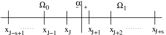This subsection deals with the time-marching at the grid nodes where the stencil of (9) crosses $\alpha$. We define $J$ by $x_{J}\leq\alpha<x_{J+1}$, and we assume that the grid is uniform from $x_{J-s+1}$ to $x_{J+s}$ (figure 1). At the so-called irregular nodes $x_{J-s+1},...,x_{J+s}$, the scheme (9) must not be applied naïvely, for three reasons. First, the spatial derivatives of the solution are not smooth across $\alpha$, hence the order of convergence of the scheme decreases. Secondly, the subcell position of $\alpha$ inside the mesh is ignored, which leads to a $O(\Delta\,x)$ error. Thirdly, the jump conditions (1) are not enforced in the scheme. The numerical waves diffracted by the interface may therefore not tend towards the exact waves.

At the irregular nodes, we adapt an immersed interface method [21]. This method requires knowing the jump conditions satisfied by the spatial derivatives of $\boldsymbol{U}$. We deduce these conditions from (4) for all $m\geq 1$

where $\boldsymbol{D}_{m}$ is a $4\,(m+1)\times 4\,(m+1)$ matrix depending on the permeability $\kappa_{s}$ and on the physical parameters around $\alpha$. Let $k$ be a positive integer. At the $2\,k$ grid nodes surrounding $\alpha$, $2\,k$-th order Taylor expansions of $\boldsymbol{U}(x_{i},\,t_{n})$ on $\alpha^{\pm}$, together with the jump conditions (11), are written in the matrix form

where $\boldsymbol{M}$ is a $8\,k\times 8\,k$ matrix. The Taylor series remainder term is removed from (12), and the exact values are replaced by numerical ones. The spatial derivatives estimated by performing inversion of (12) are used to build smooth extensions of the solution, called modified values, on the right of $\alpha$:

where $\boldsymbol{I}_{4}$ is the $4\times 4$ identity matrix. Modified values on the left of $\alpha$ are defined similarly. They are then injected into the scheme at the irregular nodes:

where $\boldsymbol{H}_{\Omega_{0}}$ and $\boldsymbol{H}_{\Omega_{1}}$ denote the operator $\boldsymbol{H}$ with physical parameters of media $\Omega_{0}$ and $\Omega_{1}$, respectively. Some comments about the interface method:

• •

  since the jump conditions are linear, the work is mainly carried out during a preprocessing step. At each time step, only small matrix-vector products (13) are required to compute the modified values. The computational cost is therefore negligible in comparison with that of time-marching;

• •

  the matrix $\boldsymbol{M}$ in (12) depends on the jump conditions and on the position of $\alpha$ inside the mesh. Using the modified values (14) introduces into the scheme a subcell resolution of the interface, which removes the $O(\Delta\,x)$ error [21];

• •

  in the limit case where the parameters are the same on both sides of $\alpha$ and the hydraulic contact is perfect, $\boldsymbol{U}_{i}^{*}=\boldsymbol{U}_{i}^{n}$ if $k\geq s$. Consequently, we again obtain the scheme applied in homogeneous medium;

• •

  with a $r$-th order accurate scheme, the local truncation error of (14) at irregular nodes is $r$-th order if $2\,k-1\geq r$ [21]. The fourth-order ADER scheme therefore requires $k=3$. As deduced from [13], $k=2$ suffices to ensure fourth-order overall accuracy;

• •

  GKS analysis [14] has been performed in the case of inviscid fluids on a uniform grid to determine the stability of the hybrid scheme (9) and (14). This analysis is based on the possible existence of discrete increasing modes emitted solely by the interface without any incident field [24]. A parametric study showed that the hybrid scheme is stable in tests 1 and 2 presented below, whatever the position of the interface, with $k=1,2,3$.

First we consider identical media $\Omega_{0}$ linked by an imperfect hydraulic contact $\kappa_{s}=10^{-16}$ m.s^-1.Pa^-1 at $\alpha=200.67$ m. Wave conversions are shown in Figure 2-b, and a good agreement is seen between the analytical and numerical values; on this scale, the reflected fast wave is not visible. Since no contrast of Biot’s coefficients occurs, the unmodified scheme (9) without the interface method (14) would propagate the incident wave without diffraction.

Test 2 deals with media ($\Omega_{0},\Omega_{1}$) linked by a perfect hydraulic contact $1/\kappa_{s}=0$. Without using the interface method, GKS analysis and direct simulations show that the scheme is unstable and the solution grows exponentially when crossing $x=\alpha$. Figure 3-a gives the analytical and numerical values obtained. The results of convergence studies are presented in Figure 3-b. As mentioned in section 3.3, $k=2$ or $k=3$ maintain the fourth-order accuracy of the ADER scheme; $k=1$ does not suffice, leading to a rate of convergence of only 2.9.

Test 3 focuses on the homogeneous dissipative medium $\Omega_{0}$ excited by a ponctual stress source of finite duration at $x_{s}=200$ m. A direct discretization with no splitting would give $\mbox{CFL}=0.03$ (6). A snapshot of $p$ is shown in figure 4-a. Fast waves are advected rightwards and leftwards while the slow waves remain localized around $x_{s}$, and vary considerably on small spatial scales. Their numerical values are highly smeared. In figure 4-b, the coarse grid solution is compared with a solution refined 64 times around $x_{s}$. Good agreement is seen between the exact and refined numerical values.

Test 4 is performed on ($\Omega_{0},\Omega_{1}$), with $1/\kappa_{s}=0$. Two successive mesh refinements with factors 8 and 64 are used around $\alpha$. Snapshots of $p$ at $t_{1}$ and $t_{2}>t_{1}$ are shown in figure 5. During the interaction of the incident fast wave with the interface (a-c), since the slow waves have a greater amplitude than that of fast waves, they play a crucial role in the balance of momentum and mass: a poor assessment of the slow waves would invalidate that of the other ones. At $t_{2}$ (b-d), the slow waves are greatly attenuated and remain localized near $\alpha$.

Lastly, two examples of wave propagation across multiple interfaces are investigated. The media $\Omega_{0}$ and $\Omega_{1}$ are repeated alternatively. Test 5 treats the case of two interfaces, with a known analytical solution (figure 6). As in test 4, one observes the small-scale evolution of the static slow waves generated by the interfaces.

Test 6 deals with a case of 10 interfaces with randomly distributed position. Performing such a simulation has physical applications, even in 1D [17]. Figure 7 shows $\sigma$ at the initial instant (a) and after the wave has crossed the whole set of interfaces (b). For the sake of clarity, only grid refinements positions from 1 to 8 are shown.

References

- [1] M. J. Berger, Stability of interfaces with mesh refinement, Math. Comput., 45 (1985), 301-318.
- [2] M. J. Berger, R. J. LeVeque, Adaptative mesh refinement using wave-propagation algorithms for hyperbolic systems, SIAM J. Numer. Anal., 35-6 (1998), 2298-2316.
- [3] M. A. Biot, Theory of propagation of elastic waves in a fluid-saturated porous solid. I: Low-frequency range, J. Acoust. Soc. Am., 28-2 (1956), 168-178.
- [4] M. A. Biot, Theory of propagation of elastic waves in a fluid-saturated porous solid. II: High-frequency range, J. Acoust. Soc. Am., 28-2 (1956), 179-191.
- [5] T. Bourbié, O. Coussy, B. Zinszner, Acoustics of Porous Media, Gulf Publishing Company, 1987.
- [6] J. M. Carcione, H. B. Helle, Numerical solution of the poroviscoelastic wave equation on a staggered mesh, J. Comput. Phys., 154 (1999), 520-527.
- [7] J. M Carcione, G. Quiroga-Goode, Some aspects of the physics and numerical modeling of Biot compressional waves, J. Comput. Acoust., 3 (1996), 261-280.
- [8] R. N. Chandler, D. L. Johnson, The equivalence of quasi-static flow in fluid-saturated porous media and Biot’s slow wave in the limit of zero frequency, J. Appl. Phys., 52 (1981), 3391-3395.
- [9] N. Dai, A. Vafidis, E. R. Kanasewich, Wave propagation in heterogeneous porous media: a velocity-stress, finite-difference method, Geophysics, 60-2 (1995), 327-340.
- [10] A. Ezziani, Modélisation de la propagation d’ondes dans les milieux viscoélastiques et poroélastiques, PhD thesis, University Paris-Dauphine, 2005.
- [11] B. Gurevich, On ”Wave propagation in heterogeneous porous media: a velocity-stress, finite-difference method” by N. Dai, A. Vafidis, E. R. Kanasewich, Geophysics 61-4 (1996), 1230-1231.
- [12] B. Gurevich, M. Schoenberg, Interface conditions for Biot’s equations of poroelasticity, J. Acoust. Soc. Am., 105-5 (1999), 2585-2589.
- [13] B. Gustafsson, The convergence rate for difference approximations to mixed initial boundary value problems, Math. Comput., 29-130 (1975), 396-406.
- [14] B. Gustafsson, H. O. Kreiss, A. Sundström, Stability theory of difference approximations for mixed initial boundary value problems II, Math. Comput., 26-119 (1972), 649-686.
- [15] H. Haddar, J. Li, D. Matignon, Efficient solution of a wave equation with fractional order dissipative terms, Proceedings of WAVES 07 (2007), 529-531.
- [16] P. Joly, J. Rodriguez, An error analysis of conservative space-time mesh refinement methods for the one-dimensional wave equation, SIAM J. Numer. Anal., 43-2 (2005), 825-859.
- [17] B. Lenoach, 1D waves in a random poroelastic medium with large fluctuations, Waves in Random Media, 9-4 (1999), 477-487.
- [18] R. J. LeVeque, Finite Volume Methods for Hyperbolic Problems, Cambridge University Press, 2002.
- [19] F. Lörcher, C. Munz, Lax-Wendroff-type schemes of arbitrary order in several space dimensions, IMA J. Numer. Anal., (2005), 1-28.
- [20] J. F. Lu, A. Hanyga, Wave field simulation for heterogeneous porous media with singular memory drag force, J. Comput. Phys., 208 (2005), pp. 651–674.
- [21] J. Piraux, B. Lombard, A new interface method for hyperbolic problems with discontinuous coefficients: one-dimensional acoustic example, J. Comput. Phys., 168-1 (2001), 227-248.
- [22] M. Schanz, Application of 3-D time domain boundary element formulation to wave propagation in poroelastic solids, Eng. Anal. Bound. Elem., 25 (2001), 363-376.
- [23] T. Schwartzkopff, M. Dumbser, C. Munz, Fast high order ADER schemes for linear hyperbolic equations, J. Comput. Phys., 197-2 (2004), 532-539.
- [24] L. N. Trefethen, Instability of difference models for hyperbolic initial boundary value problems, Comm. Pure Appl. Math., 37 (1984), 329-367.
- [25] Y. Q. Zeng, J. Q. He, Q. H. Liu, The application of the perfectly matched layer in numerical modeling of wave propagation in poroelastic media, Geophysics 66-4 (2001), 1258-1266.
- [26] C. Zhao, W. Li, J. Wang, An explicit finite element method for Biot dynamic formulation in fluid-saturated porous media and its application to a rigid foundation, J. Sound. Vib., 282 (2005), 1169-1181.