CPHT RR-164.1107
LPT–Orsay 07/122
hep-th/yymmnnn
November 2007
Moduli stabilization with Fayet-Iliopoulos uplift
E. Dudas1,2, Y. Mambrini2, S. Pokorski3 and A. Romagnoni2,1
1 CPhT, Ecole Polytechnique 91128 Palaiseau Cedex, France
2 Laboratoire de Physique Théorique, Université Paris-Sud, F-91405 Orsay, France
3 Institute of Theoretical Physics, Warsaw University, Hoza 69, 00-681 Warsaw, Poland
Abstract
In the recent years, phenomenological models of moduli stabilization were proposed, where the dynamics of the stabilization is essentially supersymmetric, whereas an O’Rafearthaigh supersymmetry breaking sector is responsible for the ”uplift” of the cosmological constant to zero. We investigate the case where the uplift is provided by a Fayet-Iliopoulos sector. We find that in this case the modulus contribution to supersymmetry breaking is larger than in the previous models. A first consequence of this class of constructions is for gauginos, which are heavier compared to previous models. In some of our explicit examples, due to a non-standard gauge-mediation type negative contribution to scalars masses, the whole superpartner spectrum can be efficiently compressed at low-energy. This provides an original phenomenology testable at the LHC, in particular sleptons are generically heavier than the squarks.
1 Introduction
Recently, Kachru et al. [1] proposed a strategy to stabilize the moduli in the context of type IIB string theory orientifold, following earlier work [2]. The KKLT set–up involves three steps to achieve a SUSY breaking Minkowski vacuum, while stabilizing all moduli. We will consider in this study a KKLT–like model where all the complex-structure moduli are fixed by the introduction of background fluxes for NS and RR forms. All steps except the last one (uplifting through the addition of one anti D3-brane, analyzed in detail in [3]) can be understood within the context of an effective supergravity. Whereas several attempts [4] tried to use the D-term to uplift the supersymmetric minima, it was shown that this can work only for a gravitino mass of the order of the GUT scale. It was however possible to obtain TeV gravitino mass by introducing corrections to the Kahler metric [5, 6]. Other works insisted on the possibility of using F-terms of matter fields in a decoupled sector to uplift the anti-de Sitter minima through metastable vacua [7, 8, 9].
In this note we describe a new way to obtain de Sitter space with a TeV gravitino mass by using a Fayet-Iliopoulos (FI) model [10] as uplift sector. The uplifting is realized through the appearance of a non-zero -term induced by the ’s of matter-fields charged under an anomalous U(1)X. The F-term is directly induced through the D-term contribution in the minimization procedure. Moreover, the U(1)X invariance of the superpotential implies a natural coupling between the moduli fields and the matter charged fields under the U(1)X, which changes substantially the pattern of soft breaking mass terms compared to KKLT. The framework can be naturally realized in orientifolds with internal magnetic fields and is simple enough to be able to address detailed phenomenological questions. One of the main advantages compared to previous uplifts [3, 8, 9] is a larger contribution of the modulus to supersymmetry breaking, which increases the tree-level gaugino masses. Moreover, due to the details of the model mostly related to anomaly cancelation, it is natural to introduce messenger-like fields which realize a very particular version of the gauge mediation proposed some time ago by Poppitz and Trivedi [11] (see also [12]), in which gauge mediation contributions to scalar masses are negative. This naturally leads us to a mixed gravity-gauge mediation scenario, where gauge contributions of a non-standard type [11] are generated at high scale and compete with the gravity contributions. The resulting soft spectrum at low-energy has new features compared to other supersymmetry breaking schemes, in particular the spectrum is compressed, i.e. gauginos and scalar masses have values closer to each other than in mSUGRA, gauge mediation or the mixed modulus-anomaly mediation. For related phenomenological analysis of string compactifications with stabilized moduli, see e.g. [13]. The plan of our paper is the following. In Section 2 we review the various uplift mechanisms, insisting on the (non)decoupling of the sector realizing the cancelation of the cosmological constant. In Section 3 we define our working model, based on a FI sector with an anomalous gauge symmetry, and analyze its vacuum structure. Section 4 presents a microscopic realization in terms of string orientifold models with internal magnetic fields and invoking stringy and spacetime instantons effects in order to obtain the main couplings of our model. In Section 5 we couple our supersymmetry breaking sector to MSSM and analyze the resulting superpartner spectrum at high and low-energy from the viewpoint of electroweak symmetry breaking. In Section 6, by using anomaly cancelation arguments, we enlarge our model by adding messenger like fields, chiral with respect to the symmetry. The messenger fields have a peculiar spectrum, in particular and will generate, via gauge mediation diagrams, non-standard gauge contributions [11], which will change the low-energy spectrum in an interesting way. We end with some brief summary of results and conclusions. The appendix contain a more detailed derivation of the crucial term coupling the SUSY breaking sector to the modulus sector.
2 Uplifting and decoupling
The philosophy advocated in [1] to stabilize moduli with zero cosmological constant was to separate the process into three steps :
- •
Add all possible fluxes in order to stabilize most of the (in type II, the dilaton and the complex) moduli fields.
- •
Add additional (nonperturbative in type IIB) effects in order to stabilize the remaining (Kahler moduli in type II) moduli. The corresponding dynamics is supersymmetric, generically generating a negative cosmological constant.
- •
Uplift the vacuum energy to zero by a source of supersymmetry breaking which perturbes only slightly the steps above.
The last step was realized originally in [1] by adding an anti D3 brane at the end of the throat in the internal manifold, while later on it was argued [7, 8] and explicitly shown [9] that this can be naturally realized with the help of a decoupled sector breaking dynamical supersymmetry in the rigid limit. In its manifestly supersymmetric realization, by denoting collectively the moduli left unstabilized after the first above and by the fields responsible for dynamical supersymmetry breaking and the uplift of the vacuum energy
| (1) |
the decoupling of the two sectors is symbolically described in an effective supergravity action by writing
| (2) |
The result of this decoupling is the generation of the scalar potential of the form
| (3) |
where the index depends on details of the uplift sector and the term represents the first term in an expansion which mixes non-trivially, due to supergravity interactions, the modulus sector with the uplift sector. For the case of interest , the decoupling is very efficient and has the main consequence of perturbing very little the supersymmetric modulus stabilization dynamics. This reflects itself in the very small contribution of the modulus to supersymmetry breaking, which was estimated in [9], for the case of one modulus, to be
| (4) |
The small contribution of the modulus to supersymmetry breaking in this class of uplifting mechanism has the important outcome that generically the gauginos are much lighter than the gravitino [3, 9]. Consequently, in order to find accurate predictions, one-loop contributions, in particular the anomaly-mediated ones are needed, resulting in the so-called mirage unification of gaugino masses.
It was clear from the very beginning that, while such a decoupling renders the uplifting easy to realize, it is by no means mandatory for the stabilization with zero vacuum energy. It is indeed conceivable to contemplate the possibility of a sector breaking supersymmetry that, due to various reasons, in particular gauge invariance consistency constraints, has a non-trivial coupling to the modulus (KKLT) sector. This non-decoupling was actually forced upon us by gauge invariance in the D-term attempts to uplift the vacuum energy [4], having as a result a very heavy gravitino mass. Notice that in the original version with anti D3 branes [1], a naive attempt to couple more strongly the two sectors by increasing results actually in a run-away potential which destroys the minimum.
In the next sections we provide explicit examples where this non-decoupling is successfully realized11 1 Recently, another example of non-decoupled sectors was provided in the context of heterotic strings in [14]. . Similarly to the D-term uplifting models, the non-decoupling is unavoidable due to gauge invariance constraints. In the present case, due to the use of a FI uplift sector, the novelty is the presence of a new supersymmetry breaking source which generates a positive vacuum energy, similar to the F-term uplifting models [8, 9]. As a result, compared to (4), we get a modulus contribution to SUSY breaking bigger than in [8, 9] by a factor , where is a charge that will be defined more precisely later on.
3 The model and its vacuum structure
Our model in its globally supersymmetric limit is a variant of the Fayet-Iliopoulos model of supersymmetry breaking. It has two charged fields of charges , a constant term relevant, as usual, for the supergravity generalization, and a new term parametrized by a constant which couples to the modulus under consideration . This last term is the main novelty and ensure the gauge invariance of the nonperturbative superpotential term. In the language of Supergravity (SUGRA), we consider the gauge invariant superpotential
| (5) |
where is an effective parameter coming from having integrated out all complex structure moduli through the use of fluxes, and a Fayet-Iliopoulos (FI) term generated in the 4D effective action of the form22 2 The exact form of the D-term depends in principle on the precise form of the Kahler metric. We take in what follows, but we will comment later on about other options in the analysis. The term can be interpreted as if the FI term arises from non–trivial fluxes for the gauge fields living on the –branes.
| (6) |
The non–perturbative potential is either generated by Euclidean D3-branes or by gaugino condensation [15] . The charged field restores the gauge invariance of the nonperturbative modulus-dependent superpotential [16, 17, 18].
Indeed, the gauge transformations act on various fields as
| (7) |
where are the charges of the fields . Gauge invariance forces the Kahler potential for the modulus to be of the form . This leads in turn to the FI term
| (8) |
and fixes . From Eq. (5), it is clear that imposing ensures the gauge invariance of the model. The numerical values we will be interested in what follows are
| (9) |
The first requirement in (9) is natural from the string theory viewpoint, whereas the third relation is needed in order to get TeV ; the landscape picture of string theory could be invoked in order to achieve this [1]. The smallness of the mass term in our model is then an outcome from a proper cancellation (uplift) of the cosmological constant. The most natural explanation for it, in our opinion, is in terms of stringy instanton effects recently discussed in the literature [19], which can provide values , where is the area of the euclidian brane responsible for the mass term.
From Eq. (5) we can deduce explicitly the F-part of the scalar potential given by
| (10) |
where is the inverse of the metric and is the Kahler covariant derivative : . Using a conventional Kahler potential of the form , we can rewrite Eq. (10) as33 3 The Kahler metric of the charged fields can be more complicated and can also depend on . We checked that the results do not change significantly when a more general Kahler potential is considered. :
| (11) |
The scalar potential is given explicitly as
| (12) | |||||
The nonperturbative term has significant consequences both on the resolution of the equation of motion for and , and on the uplifting mechanism. It is important to notice here that due to the intricate coupling between and , in solving the equations of motions, we cannot neglect the supergravity corrections to and in the scalar potential. In what follows we define as usual
| (13) |
Asking for a zero cosmological constant at the minimum, we can find immediately a relation at first order between the gravitino mass and the parameters of the model by anticipating that the uplift is mainly induced by :
| (14) |
Solving now the equations , using the approximations allowed by the choice of the parameters, and always fixing the cosmological constant to zero, we obtain at the first order 44 4 For simplicity, we take all the parameters to be real and we choose the real positive solution for the vev of . The general case of complex parameters does not change significantly the results.
| (15) | |||||
| (16) | |||||
| (17) |
We can check our approximation by defining a parameter which will be fundamental in the calculation of the soft breaking term. measures the contribution of to the uplift :
| (18) |
Solving with the reasonable hypothesis55 5 If the conditions (19) are violated, it turns out not to be possible to realize the uplift of the cosmological constant with a TeV gravitino mass.
| (19) |
and (hypothesis that we check aposteriori), we obtain at first order
| (20) |
which gives for a typical KKLT value , and which is bigger than the values obtained in sequestered F-term uplifting [9], where
| (21) |
It turns out that the numerical solution of the equation of motion for is very close to the supersymmetric minimum for , whereas the numerical solutions for , are very close to the analytical ones (16), (17) ; the deviation from it can be parameterized by expanding in a perturbative parameter of the theory (which is in our specific case), checking in the meantime the analytical consistency of the whole procedure. In fact, this procedure is remnant of the one used in the original KKLT paper where the authors noticed that the term induced by the anti D3–brane which is proportional to , does uplift the potential without disturbing significantly the shape and the value of at the minimum. F–term uplifting exhibit similar features in the sense that it can be seen (see Eq. (11)) as an uplift proportional to . However, it is important to point two main differences with KKLT models [1] and F-term uplifting ones [8, 9]. Indeed, firstly the F-term breaking parameters are induced by the D-term, which imposes a non vanishing vev for and especially at the minimum of the potential. Secondly, the gauge invariant term in imposes more constraints on the parameter space, linking directly the and in the minimization procedure. It turns out that is more important in this case and participate more to the cosmological constant cancelation. One of the main consequences appears on the gaugino masses (), which are heavier than in previous uplift schemes. One of the main difference with the models inspired by D-term uplifting is the possibility to achieve a TeV scale SUSY breaking.
At the first order, the value of at the minimum respects the condition , i.e.
| (22) |
The mass of the gravitino is given by . To illustrate the procedure, we apply the minimization condition to find a phenomenological viable point in the parameter space. We fix , and . is given by the gauge invariance constraint, (and ) are obtained by the minimization procedure, whereas is fine-tuned to ensure a zero cosmological constant. For the numerical values provided in Fig. 1, we obtain :
| (23) |
Concerning the contribution of various fields to the uplift, we obtain and .


4 Microscopic definition of the model
The setup we are considering is very similar to the one proposed in [20, 18, 4], with slight modifications. We start with type IIB string propagating on a Calabi-Yau manifold, orientifolded with an involution , which generate non-dynamical O7 and O3 orientifold planes. They ask for consistency the introduction of D7 and D3 branes. The non-trivial dynamics we will be concerned happen on the D7 branes. The relevant ingredients for our discussion are two stacks of D7(1) and D7(N) branes , giving rise to an and an gauge groups. The stack D7(N) wraps a four-cycle of volume , which suitably combined with an axion obtained by wrapping the RR four-form over the four-cycle , forms the complex Kahler modulus . The massless chiral open string spectrum for an arbitrary number of stacks of branes can be given a more geometrical interpretation by performing three T-dualites in a IIA setting with intersecting D6(a) branes [22]. In IIA orientifolds with D6 branes at angles, each stack , containing coincident branes, has a mirror with respect to the O6 planes. The chiral spectrum for type II orientifold Calabi-Yau compactification with intersecting branes contains chiral fermions in
| (24) |
where is the intersection number between the stacks
and , is the intersection number between the images
and , whereas is the intersection number between the
stack and the O6 planes. In the original type II language,
the intersection numbers are mapped into magnetic fluxes
[21, 22].
For the two stack case discussed above and in the type IIA picture,
we take the brane to intersect along a six-dimensional subspace with
the O-planes. This means that the spectrum of the states stretched
between the brane and its image is non-chiral and is
described in four-dimensional language by fields of
charges . We take the multiplicity of these states,
which correspond to the symmetric representations in (24), to
be equal to one. If the second stack does not intersect the
O-planes, the symmetric/antisymmetric representations are absent and
only the byfundamental chiral multiplets and , of multiplicity , are charged under the non-abelian gauge group.
In the type IIB language, the axion field coupling to the gauge
fields get charged under the gauge field of the first stack if
the two stacks intersect over a two-dimensional cycle on which the
magnetic flux is non-trivial [23]. In this case we get
the typical Stueckelberg couplings
| (25) |
rendering the gauge field massive. The supersymmetric description of this phenomenon is precisely the one described in eqs. (6)-(8).
If , the non-abelian stack will undergo gaugino condensation and generate a non-perturbative ADS type superpotential in terms of the ”mesonic” fields .
| (26) |
It was shown long ago in a similar heterotic context [16] and updated recently for orientifolds [18, 4, 23] that, once the Green-Schwarz anomaly cancelation conditions are imposed, the charges of the mesons are precisely such that the gauge variation of in (26) is compensated by that of the mesons. In addition to the D-term potential (6) and the nonperturbative term (26), the other terms in the superpotential defining our model are
| (27) |
The constant can be generated by closed string three-form fluxes [2, 1] which stabilize the dilaton and the complex structure moduli, whereas the second term in (27) is a disk-level perturbative open string coupling. The last term, which will turn out to be crucial for our purposes, deserves a special discussion. Unless the stack and its image are parallel to each other in some internal subspace, the mass cannot have a perturbative origin (like for example Wilson lines). In what follows we will advocate a non-perturbative origin . There are two possibilities for generating an exponentially small mass term . The first option is provided by stringy instanton effects [19]. The instantons under consideration can be E instantons or E3 instantons wrapping cycles different than the one defining the Kahler modulus under consideration. The resulting parameter m is then proportional to , where is the instanton action. The other option uses a second sector undergoing spacetime nonperturbative dynamics. This could arises, for example, if the brane is part of a bigger stack of branes , with the non-abelian part undergoing non-perturbative phenomena, for example gaugino condensation . Then an open string perturbative coupling
| (28) |
generates a hierarchically small mass parameter . Whereas it is fair to say that constructing a complete, global model along these lines could be a difficult task, there is no conceptual obstruction to the implementation of the ingredients that we need in order to define completely our model in a semi-realistic compactification.
Finally, by invoking the stringy instanton effects described previously or, alternatively, by integrating out the quarks of the hidden sector as described in detail in the Appendix, we arrive at the generic form of the superpotential
| (29) |
that was defining our model analyzed in the previous Section.
5 Soft–breaking terms
In what follows we investigate the effects of supersymmetry breaking in the observable sector, that we take for simplicity to be the Minimal Supersymmetric Standard Model (MSSM). Irrespective on which type of brane MSSM sit (D7 or D3 branes), if they contain magnetic fluxes the gauge kinetic functions contain a T-dependence
| (30) |
where are positive numbers66 6 In the rest of the paper we consider . This is easier to obtain in a string setup and also safer for phenomenological purposes, since for there is a serious danger of destabilizing the vacuum. and effective constants generated by the couplings of the MSSM branes to other, stabilized fluxes (e.g. the dilaton ). By denoting in what follows by matter fields and by greek indices any field contributing to SUSY breaking, a relevant quantity for computing the soft terms [24] is the coupling of the matter fields metric to the SUSY breaking fields. This can in turn be parameterized as
| (31) |
where , , and representing the matter fields, not participating to the SUSY breaking mechanism (). The metric in (31) is written as an expansion in powers of the charged vev fields , up the quadratic order.
5.1 Scalar masses
For the calculation of the scalar mass, we use the classical formulas at the linear order in the D-term [18, 25]
| (32) |
with the standard definitions
| (33) |
For the uncharged77 7 We anticipate, for reasons that we discuss later on, that the MSSM fields are neutral with respect to the symmetry. scalar mass terms we obtain, after normalization of the kinetic terms :
| (34) |
Notice that the contribution to the scalar masses coming from the moduli, depending on the unknown moduli weights , is suppressed compared to the universal first term. This comes actually from the uplift field , via the purely supergravity interactions, as in the mSUGRA case . The third term, coming from the main uplift field , is also negligibly small if , whereas it is comparable to the universal contribution for and dominant for . Whereas this last case cannot arise in a string compactification, the case could and deserve a more detailed study from the viewpoint of possible flavor-dependent couplings. Since is a charged and therefore open-string/brane-localized field, whereas the modulus is a closed/bulk field, the pattern of the flavor dependence of their respective couplings to MSSM fields is clearly different. In particular, whereas it is very difficult to supresss the mixed modulus-MSSM fields couplings (first term in the rhs of (31)) in the Kahler potential, this can be easily realized for the uplift open field (the second term in the rhs of (31)) 88 8 These comments also apply to a generic F-term uplift [8, 9].. In this last case (or if the couplings are flavor-universal), the scalar masses (34) do not generate dangerous FCNC effects. In conclusion, under reasonable assumptions, the dependence of the soft masses on the unknown quantities is weak and can be neglected in a first approximation. For the phenomenological analysis performed in the next section we analyze in detail the universal case, where the gravity-mediated contributions are dominated by the universal term .
5.2 Gaugino masses
The gaugino mass for a general gauge kinetic function is given by [25]:
| (35) |
With the hypothesis of a gauge kinetic function given in (30), we obtain
| (36) |
where
| (37) |
For the phenomenological analysis performed in the next section we analyze in detail the unified case , which is easily realized for .
5.3 Trilinear couplings
The general formulas for the trilinear couplings including the D-term contribution can be found in [18, 25]
| (38) |
where , , etc. It is easy to show that the last contribution in (38) coming from the D-term is in our case negligible. Applying it to our special case, after normalization of the kinetic terms and for a typical superpotential for matter fields of the form , we get
| (39) | |||||
where symm. denotes the symmetrized parts in the (KLM) indices and
| (40) |
are the low-energy (for canonically normalized fields) Yukawa couplings.
Comments similar to the ones concerning the flavor-dependence of soft masses apply here. Analogously to the discussion concerning soft scalar masses, the dependence of trilinear -couplings on the unknown quantities can be neglected under reasonable assumptions. For the phenomenological analysis performed in the next section we analyze in detail the gravity-universal case .
5.4 and terms
The parameter and bilinear coupling arises in our model through a Giudice-Masiero mechanism [26]. We will suppose a Kahler metric of the form
| (41) |
where is a modular function ensuring the modular invariance of the term . With this convention, we can deduce
| (42) |
with in our case. The modular function allows a certain flexibility of and terms with respect to the gravitino mass. We will use this flexibility in order to determine the appropriate parameters from the analysis of electroweak symmetry breaking in the next section.
5.5 Phenomenology
If we apply the previous soft term calculations to the numerical example of Eq. (23) we obtain TeV and GeV. In this case, we have a splitting (a factor 10) between scalar masses and gaugino masses , smaller by a factor of two than in the classical KKLT case. This implies that the one loop contributions (AMSB) are less important here compared to the tree-level one. As we already mentioned, this comes from the fact that participate more actively to the SUSY breaking and therefore its contribution to the gaugino masses is more important compared to the KKLT or classical F-term uplifting cases. We show the spectrum of some typical points in table 1. The absolute value of is determined by the minimisation condition of the Higgs potential (assuming CP conservation), but its sign is not fixed. Furthermore, instead of it is more convenient to use the low energy parameter , which is a function of and the other parameters. The low energy mass spectrum is calculated using the Fortran package SUSPECT [37] and its routines were described in detail in ref. [37]. The evaluation of the branching ratio, the anomalous moment of the muon and the relic neutralino density is carried out using the routines provided the program micrOMEGAs2.0 [38]. Minimizing the Higgs potential in the MSSM leads to the standard relation
| (43) |
This minimization condition is imposed at the scale . Eq. (43) can be approximated in most cases by
| (44) |
When the right hand side is negative, electroweak breaking cannot occur. The Higgs mass parameter is positive at the GUT scale, but decreases with decreasing scale down to , through the contributions it receives from RG running, . Typically, the value of at the scale depends mainly on the soft breaking terms and .
| A | B | |
| 1 | 1 | |
| 0.3 | 0.5 | |
| 1 | 1 | |
| 30 | 15 | |
| 98.3 | 59.4 | |
| (GeV) | 810 | 1070 |
| 113 | 145 | |
| 224 | 286 | |
| 762 | 948 | |
| 118.7 | 120.1 | |
| 2220 | 3291 | |
| 1385 | 1770 | |
| 1918 | 2612 | |
| 2577 | 3302 | |
| 1913 | 2610 | |
| 2313 | 3226 | |
| 2578 | 3303 | |
| 2288 | 3198 | |
| 2424 | 3235 | |
| 2553 | 3275 |
| A+GMSB | B+GMSB | |
| 1 | 1 | |
| 0.3 | 0.5 | |
| 1 | 1 | |
| 30 | 15 | |
| 97.3 | 59.4 | |
| 6 | 6 | |
| (GeV) | 186 | 216 |
| 117 | 152 | |
| 165 | 201 | |
| 848 | 1057 | |
| 119.7 | 121.1 | |
| 1744 | 2769 | |
| 993 | 1225 | |
| 1281 | 1713 | |
| 1951 | 2417 | |
| 1251 | 1701 | |
| 1932 | 2686 | |
| 1952 | 2418 | |
| 2128 | 2872 | |
| 2164 | 2963 | |
| 2292 | 2912 | |
| 0.122 | 0.117 |
6 Anomalies and Gauge Messengers
6.1 Anomalies and messengers
Anomaly arguments that we discussed in Section 3 and coupling of the MSSM gauge couplings to the T-modulus introduced in the previous section strongly suggest that there should be fields carrying Standard Model quantum numbers charged under the additional . Indeed, the couplings (30) generate, through the shift of T under gauge transformation (7) mixed anomalies, with being a SM group factor. These anomalies imply some SM-charged fields have to carry positive (for positive coefficients in (30)) charges in order to cancel, via the 4d Green-Schwarz mechanism, the mixed anomalies. There are two generic possibilities that realize this, that we consider in turn :
- •
The SM quarks and leptons carry charges. In this case, the squarks and the sleptons will acquire D-term soft masses TeV. If we wish to keep some light superpartners and to minimize the fine-tuning of the electroweak scale, one possibility would be to give a charge to the first two generations only [34]. The large hierarchy betwen the first two and the third generation of squarks can generate various problems, in particular the third generation could become tachyonic through the RGE running towards low-energy [35].
- •
All MSSM fields (quarks, leptons and Higgses ) carry no charges. In this case, there should be additional fields carrying both SM and charges. In order to preserve perturbative gauge coupling unification and be able to give these states a large mass, we only consider complete vector-like multiplets, called generically and in what follows. Notice that these fields have precisely the features of the so-called ”messenger” fields in gauge-mediation scenarios [28].
These arguments strongly suggest therefore to introduce heavy messengers which can contribute significantly to the soft SUSY masses breaking terms. In our model, coupling the charged field to the messengers pushes naturally the messenger scale up to the GUT scale, still giving rise to important contributions to the scalar masses.
The superpotential is of the form :
| (45) |
where and represent the messenger fields of charges and respectively. Without loss of generality, we will take thorough the rest of the analysis. Notice that the messenger fields, vector-like wrt to SM gauge interactions, are chiral wrt the anomalous symmetry. In (45), is the low-energy coupling, related to the high-energy supergravity coupling by a formula similar to (40). Notice that for zero (or positive) modular weights for , , , the low energy coupling is highly suppressed wrt the high-energy ones by inverse powers of .
In general, adding messengers to a supersymmetry breaking sector generates a new, supersymmetry preserving vacuum. This is because in order to generate gaugino masses we have to explicitly break R-symmetry, which in turns generically restores supersymmetry [36]. In our case, however, due to the presence of the gauge symmetry, this does not happen ; even in the presence of messenger fields, there is no supersymmetry preserving vacuum. This is an important difference compared to standard gauge mediation models of supersymmetry breaking.
Another very important outcome of the charged nature of messenger fields is a new D-term contribution to scalar messenger masses.
The scalar messenger mass matrix is
| (46) |
Once diagonalized the messenger scalar mass matrix, the two eigenvalues are :
| (47) |
whereas the fermion mass is given by :
| (48) |
Notice that
| (49) |
By standard gauge-mediation type diagrams, gaugino masses are induced at one-loop, whereas scalar masses are induced at two-loops. Due to (49), the computation of the scalar masses is slightly different compared to the standard gauge-mediation models, as shown by Poppitz and Trivedi [11]. In particular the result is not anymore UV finite, there is a logarithmically divergence term which will play a crucial role in what follows.
In the context of our model, the uplift relation (14) has
very strong phenomenological implications.
Indeed, if D-term contributions appear in the scalar soft mass
terms of the visible sector, through the two loops–suppressed GMSB
mechanism , it turn out that their magnitude is automatically of the
same order as the gravity (i.e. ) contribution.
This is clearly seen from our numerical example (23), in
particular from the values of the -term.
6.2 Soft masses
The exact calculation of the radiatively induced gaugino and scalar masses is performed in [11, 28]. For one messenger multiplet, we obtain for the gaugino mass
| (50) |
and for the scalar masses
| (51) |
with and where is the corresponding SM gauge coupling (unified at high scale), is the Casimir in the MSSM scalar fields representations (normalized as for the fundamental representation of gauge group, while for it is simply ) and the Dynkin index of the messenger representation (normalized to 1/2 for a fundamental of ). The function is given by
| (52) | |||||
where
| (53) | |||||
above refers to the dilogarithm function and is defined by . After an expansion in the perturbative parameter the mass terms become
| (54) |
where is the low-energy mass parameter of the FI model, equal to for our model in Section 3, and
| (55) | |||||
where in the last line we used (15).
One important feature of Eq.(55) is the presence of the term in the soft scalar masses. This logarithmic divergence arises typically in the presence of anomalous that gives a non-vanishing supertrace (49) for the messengers superfields [11]. In low energy-GMSB, it usually limits the scale beyond which ”new physics” occurs, because the scalars become tachyonic already for around 50. In our specific case, the running is much shorter : from the FI scale () to the Planck scale (a factor less than 10).
Some remarks are in order concerning the anomaly-mediation contribution to soft terms. For scalar masses, they are completely negligible compared to both gravity and the non-standard GMSB contributions (55). For gaugino masses, they are much smaller than the gravity contribution, whereas they are suppressed wrt to the standard GMSB contributions (54) only by the number of messenger fields . Since we consider relatively large values in our analysis, we can neglect also the anomaly contributions to gaugino masses in what follows.
6.3 Phenomenological effects
In the complete model, scalar and gaugino masses get contributions both from gravity and the gauge mediation diagrams
| (56) |
The negative contribution to the scalar masses induced by the ultraviolet divergence has strong consequences on the mass spectrum and the phenomenology of the model. It reduces significantly the masses in the left–handed squark sector (the more charged under the SM gauge group) and can have repercussion in the neutralino sector through . In addition, decreasing the value of and with gauge mediation naturally decreases the value of through Eq.(44).
We show in Tab.(2) (Tab.(1)) the spectrum with (without) the gauge mediation contributions, after including the RG evolution to low-energy. The scalar spectrum and nature of neutralino (through the parameter) are considerably altered. On the other hand, the positive GMSB contribution to gauginos compresses even more the supersymmetric spectrum, especially for a large number of messenger fields. Notice that, whereas for traditional messenger masses (i.e. around TeV), the RG running up to the unification scale forces in order to avoid strong coupling effects, in our case since messengers have masses of order GeV, the number of messengers can be larger. By using this (and/or also the alternative possibility of enhancing the negative contribution to scalar masses by decreasing the coupling ) we can obtain the efficiently compressed spectrum displayed in Table 2.
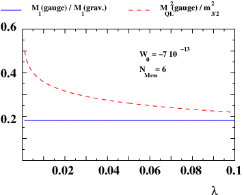
Notice that, in contrast to other scenarios (see for example [27] ) where the gauge/gravity relative contributions are completely fixed, in our case, due to the presence of the two charged fields , the gauge and the gravity contributions to soft terms are governed by different parameters. It is instructive to see in Figs.(2) the dependence of the gauge contribution to soft terms as a function of the relevant parameters of the model ( and ). For low values of , the gauge contribution to the scalar mass becomes important, and even of the same order of magnitude than the gravity contribution for . Indeed, smaller values of implies lighter messenger and thus a larger running between and . Gaugino masses are not affected by . The number of messenger acts directly on the scalar and gaugino masses, and the gauge contribution becomes relevant in both cases for .

7 Conclusions
In this work, we tried to combine the various ingredients that a microscopic string theory can provide in order to successfully stabilize moduli fields with a TeV gravitino mass. This is realized via a supergravity version of the Fayet-Iliopoulos (FI) model with an anomalous gauge symmetry, in which a (non-linearly charged) modulus field plays an instrumental role, whereas in turn the FI sector plays a crucial role in supersymmetry breaking and for getting a zero vacuum energy. Due to the non-decoupling between the modulus and the uplift sector, the contribution of the modulus to supersymmetry breaking is higher than in previous schemes. This increases the numerical values of the gaugino mass and renders less important the loop contributions to soft terms.
Due to the intrincate definition of the model, anomaly arguments strongly suggests the presence in the spectrum of charged fields which have properties similar to messenger fields of gauge mediation of supersymmetry breaking. Due to the charged nature of our messengers, their superpotential couplings are R-symmetric. As a consequence, in contrast to standard gauge mediation scenarios, our messengers do not restore supersymmetry ; there is no new supersymmetric vacuum state due to their presence and couplings. Our model has therefore a completely stable non-supersymmetric ground state, which is difficult to realize in more standard gauge-mediation scenarios. Whereas, for the standard reasons, our messengers are vector-like with respect to SM gauge interactions, due to anomaly cancellations they are however chiral with respect to the interactions. Consequently, due to their coupling to the FI supersymmetry breaking sector, they have a particular spectrum, in particular . The resulting mixed gravity/gauge mediation scenario is therefore of non-standard type : the two-loop gauge mediation contributions to MSSM scalars are negative [11, 12].
The mass scales in the problem are such that gravity and gauge mediation contributions to scalar soft masses are comparable and compete with each other, providing an original predictive spectrum and phenomenology. Indeed, squarks, which are the heaviest superpartners in most mediation scenarios, are here typically the lightest scalars since they get the biggest negative contributions from the non-standard gauge-mediation contribution (55). Taking into account the larger than usual gravity-induced gaugino masses and the additional positive contribution to them coming from gauge mediation diagrams, we end up with an original low-energy spectrum in which the whole superpartners spectrum is more compressed than in the usual mSUGRA, gauge or mixed modulus-anomaly mediation scenarios. The complete mixed model of Section 6 has the Higgsinos as the LSP and a good relic abundance, compatible with the WMAP bounds. The peculiar details of the spectrum, like the universality of gaugino masses at the unification scale and the negative GMSB contribution to scalar masses, rendering squarks lighter than sleptons, could be tested at LHC and certainly deserve a more focused study.
Finally, whereas in the present paper we get a bigger modulus contribution to supersymmetry breaking than in previous O’Rafeartaigh type models, the main contribution still comes from the uplift sector and more precisely in our case from the field. It is a very interesting and open question to find explicit realizations, with complete moduli stabilization and zero vacuum energy, of the string-inspired supersymmetry breaking parametrizations [25], which assumes moduli/dilaton domination. To our knowledge, this does not seem to be realized in the current known models of moduli stabilization.
8 Appendix : Dynamical origin for the superpotential
The aim of this appendix is to justify the coupling
| (57) |
that we considered in the superpotential of our model. We will show that this
term has its origin in strong coupling regime effects for the non-abelian
gauge group of the hidden sector, and that in particular it is induced by
”integrating out” the mesonic fields which are the right degrees of
freedom describing the theory in such regime.
As discussed in section 4, the microscopic description of the
model implies chiral multiplets in the representions
and of the gauge group .
Naturally, at a characteristic scale
| (58) |
the non-abelian gauge group will enter in a strong coupling regime, it will undergo a gaugino condensation and the model is properly described in terms of the mesonic field , of generic charge under the gauge group (once normalized at the charge of the field ). A non-perturbative ADS potential is generated:
| (59) |
Including the most general disk-level perturbative open string coupling, and the coupling between and discussed in section 4, the gauge invariant superpotential reads 99 9 For the aim of this appendix, the term is completely irrelevant.
| (60) |
The auxiliary fields and the D-term can now be calculated [16]:
| (61) |
From a simple analysis of the equations of motions for the mesons, and , it is possible to see that in the minimum, under the conditions
| (62) |
and in particular requiring 1010 10 This in order to assure that ,in accord with what happens in the usual FI global model.
| (63) |
the contribution of the D-term is negligible, and the value of the F-terms for the mesons are very small. These F-terms satisfy the relation
| (64) |
Since in the potential the contributions of these F-terms are respectively proportional to and , as long as the vev’s for the mesons is very small compared to , we are therefore allowed to integrate out the mesons and the effective superpotential we obtain has the form
| (65) |
Nonetheless, as one can show resolving in the first approximation the equation , the vev of the meson is approximatively
| (66) |
and then, using (63) and , we have
| (67) |
Therefore, for small enough (62) and for reasonable , this ratio is actually and the ”integration out” is consistent. By re-writing the superpotential (65) by using the definitions
| (68) |
we find exactly the form of the superpotential used in the equation
(5) once the right powers of restored.
As a numerical example, in order to check if the results obtained in the
paper agree with a reasonable nonperturbative scale , we can
consider the special case , i.e. the case studied numerically in the
section 5.5. With the choice of the parameters done in that
example, we can evaluate
| (69) |
which means that in this scenario we expect that the non-abelian gauge group enters in a strong coupling regime at a sensible scale of order GeV. Moreover, we can check if in this case the approximations done for the ”integration out” step are good. Actually, since and , it is clear that (67) is verified and that therefore the whole procedure is consistent.
Acknowledgments
Work partially supported by the CNRS PICS # 2530 and 3059, RTN contracts MRTN-CT-2004-005104 and MRTN-CT-2004-503369, the European Union Excellence Grant, MEXT-CT-2003-509661 and the European contract MTKD-CT-2005-029466. E.D. would like to thanks the Institute for Theoretical Physics of Warsaw form warm hospitality and financial support via the ”Marie Curie Host Fellowship for Transfer of Knowledge” MTKD-CT-2005-029466. The work of Y.M. is sponsored by the PAI programm PICASSO under contract PAI–10825VF. He would like to thank the European Network of Theoretical Astroparticle Physics ILIAS/N6 under contract number RII3-CT-2004-506222 and the French ANR project PHYS@COLCOS for financial support. The work of A.R. was partially supported by INFN and by the European Commission Marie Curie Intra-European Fellowships under the contract N 041443. The authors want to thank Chloé Papineau, Erich Poppitz, Mariano Quiros and Michele Trapletti for useful discussions. E.D. and S.P. thank the Theory Group of CERN for hospitality during the completion of this work.
References
- [1] S. Kachru, R. Kallosh, A. Linde and S. P. Trivedi, Phys. Rev. D 68 (2003) 046005 [arXiv:hep-th/0301240].
- [2] S. B. Giddings, S. Kachru and J. Polchinski, Phys. Rev. D 66 (2002) 106006 [arXiv:hep-th/0105097].
- [3] K. Choi, A. Falkowski, H. P. Nilles, M. Olechowski and S. Pokorski, JHEP 0411 (2004) 076 [arXiv:hep-th/0411066]; K. Choi, A. Falkowski, H. P. Nilles and M. Olechowski, Nucl. Phys. B 718 (2005) 113 [arXiv:hep-th/0503216]; M. Endo, M. Yamaguchi and K. Yoshioka, Phys. Rev. D 72 (2005) 015004 [arXiv:hep-ph/0504036]; A. Falkowski, O. Lebedev and Y. Mambrini, JHEP 0511 (2005) 034 [arXiv:hep-ph/0507110]; K. Choi, K. S. Jeong, T. Kobayashi and K. i. Okumura, Phys. Lett. B 633 (2006) 355 [arXiv:hep-ph/0508029]; O. Lebedev, H. P. Nilles and M. Ratz, Phys. Lett. B 636 (2006) 126 [arXiv:hep-th/0603047].
- [4] G. Villadoro and F. Zwirner, Phys. Rev. Lett. 95 (2005), 231602, [hep-th/0508167]; A. Achucarro, B. de Carlos, J. A. Casas, and L. Doplicher, JHEP 06 (2006), 014, [hep-th/0601190]; S. L. Parameswaran and A. Westphal, JHEP 10 (2006), 079, [hep-th/0602253]; E. Dudas and Y. Mambrini, JHEP 10 (2006), 044, [hep-th/0607077].
- [5] E. Dudas and M. Quiros, Nucl. Phys. B 721 (2005) 309 [arXiv:hep-th/0503157]; F. P. Correia, M. G. Schmidt and Z. Tavartkiladze, arXiv:hep-th/0602173; for earlier work, see E. Ponton and E. Poppitz, JHEP 0106 (2001) 019 [arXiv:hep-ph/0105021]; JHEP 0304 (2003) 050 [arXiv:hep-th/0209178].
- [6] V. Balasubramanian and P. Berglund, JHEP 0411 (2004) 085 [arXiv:hep-th/0408054]; V. Balasubramanian, P. Berglund, J. P. Conlon and F. Quevedo, JHEP 0503 (2005) 007 [arXiv:hep-th/0502058]; G. von Gersdorff and A. Hebecker, Phys. Lett. B 624 (2005) 270 [arXiv:hep-th/0507131]; M. Berg, M. Haack and B. Kors, Phys. Rev. Lett. 96 (2006) 021601 [arXiv:hep-th/0508171].
- [7] M. Gomez-Reino and C. A. Scrucca, JHEP 0605 (2006) 015 [arXiv:hep-th/0602246] ; JHEP 0609 (2006) 008 [arXiv:hep-th/0606273] ; JHEP 0708 (2007) 091 [arXiv:0706.2785 [hep-th]].
- [8] O. Lebedev, H. P. Nilles, and M. Ratz, Phys. Lett. B636 (2006), 126, [hep-th/0603047]; S. P. de Alwis, Phys. Lett. B 628 (2005) 183 [arXiv:hep-th/0506267].
- [9] E. Dudas, C. Papineau and S. Pokorski, JHEP 0702 (2007) 028 [arXiv:hep-th/0610297] ; H. Abe, T. Higaki, T. Kobayashi and Y. Omura, Phys. Rev. D 75 (2007) 025019 [arXiv:hep-th/0611024] ; R. Kallosh and A. Linde, JHEP 0702 (2007) 002 [arXiv:hep-th/0611183] ; O. Lebedev, V. Lowen, Y. Mambrini, H. P. Nilles and M. Ratz, JHEP 0702 (2007) 063 [arXiv:hep-ph/0612035] ; Z. Lalak, O. J. Eyton-Williams and R. Matyszkiewicz, JHEP 0705 (2007) 085 [arXiv:hep-th/0702026] ; P. Brax, A. C. Davis, S. C. Davis, R. Jeannerot and M. Postma, JHEP 0709 (2007) 125 [arXiv:0707.4583 [hep-th]].
- [10] P. Fayet and J. Iliopoulos, Phys. Lett. B 51 (1974) 461 ; P. Fayet, Phys. Lett. B 69 (1977) 489.
- [11] E. Poppitz and S. P. Trivedi, Phys. Lett. B 401 (1997) 38 [arXiv:hep-ph/9703246].
- [12] N. Arkani-Hamed, J. March-Russell and H. Murayama, Nucl. Phys. B 509 (1998) 3 [arXiv:hep-ph/9701286].
- [13] B. Acharya, K. Bobkov, G. Kane, P. Kumar and D. Vaman, Phys. Rev. Lett. 97 (2006) 191601 [arXiv:hep-th/0606262] ; B. S. Acharya, K. Bobkov, G. L. Kane, P. Kumar and J. Shao, arXiv:hep-th/0701034. ; J. P. Conlon, C. H. Kom, K. Suruliz, B. C. Allanach and F. Quevedo, JHEP 0708 (2007) 061 [arXiv:0704.3403 [hep-ph]] ; J. P. Conlon, arXiv:0710.0873 [hep-th].
- [14] M. Serone and A. Westphal, JHEP 0708 (2007) 080 [arXiv:0707.0497 [hep-th]].
- [15] H. P. Nilles, Phys. Lett. B 115 (1982) 193. S. Ferrara, L. Girardello and H. P. Nilles, Phys. Lett. B 125 (1983) 457. J. P. Derendinger, L. E. Ibanez and H. P. Nilles, Phys. Lett. B 155 (1985) 65; M. Dine, R. Rohm, N. Seiberg and E. Witten, Phys. Lett. B 156 (1985) 55.
- [16] P. Binetruy and E. Dudas, Phys. Lett. B 389 (1996) 503 [arXiv:hep-th/9607172].
- [17] N. Arkani-Hamed, M. Dine and S. P. Martin, Phys. Lett. B 431 (1998) 329 [arXiv:hep-ph/9803432].
- [18] E. Dudas and S. K. Vempati, Nucl. Phys. B 727, 139 (2005) [arXiv:hep-th/0506172].
- [19] R. Blumenhagen, M. Cvetic and T. Weigand, Nucl. Phys. B 771 (2007) 113 [arXiv:hep-th/0609191] ; L. E. Ibanez and A. M. Uranga, JHEP 0703 (2007) 052 [arXiv:hep-th/0609213].
- [20] C. P. Burgess, R. Kallosh and F. Quevedo, JHEP 0310 (2003) 056 [arXiv:hep-th/0309187].
- [21] C. Bachas, arXiv:hep-th/9503030; C. Angelantonj, I. Antoniadis, E. Dudas and A. Sagnotti, Phys. Lett. B 489 (2000) 223 [arXiv:hep-th/0007090].
- [22] M. Berkooz, M. R. Douglas and R. G. Leigh, Nucl. Phys. B 480 (1996) 265 [arXiv:hep-th/9606139]; R. Blumenhagen, L. Goerlich, B. Kors and D. Lust, JHEP 0010 (2000) 006 [arXiv:hep-th/0007024]; G. Aldazabal, S. Franco, L. E. Ibanez, R. Rabadan and A. M. Uranga, JHEP 0102 (2001) 047 [arXiv:hep-ph/0011132].
- [23] M. Haack, D. Krefl, D. Lust, A. Van Proeyen and M. Zagermann, JHEP 0701 (2007) 078 [arXiv:hep-th/0609211].
- [24] L. Girardello and M. T. Grisaru, Nucl. Phys. B 194 (1982) 65.
- [25] V. S. Kaplunovsky and J. Louis, Phys. Lett. B 306 (1993) 269 [arXiv:hep-th/9303040] ; A. Brignole, L. E. Ibanez and C. Munoz, Nucl. Phys. B 422 (1994) 125 [Erratum-ibid. B 436 (1995) 747] [arXiv:hep-ph/9308271] ; S. Ferrara, C. Kounnas and F. Zwirner, Nucl. Phys. B 429 (1994) 589 [Erratum-ibid. B 433 (1995) 255] [arXiv:hep-th/9405188].
- [26] G. F. Giudice and A. Masiero, Phys. Lett. B 206 (1988) 480.
- [27] Y. Nomura and M. Papucci, arXiv:0709.4060 [hep-ph].
- [28] G. F. Giudice and R. Rattazzi, Phys. Rept. 322 (1999) 419 [arXiv:hep-ph/9801271].
- [29] S. B. Giddings, S. Kachru and J. Polchinski, Phys. Rev. D 66 (2002) 106006 [arXiv:hep-th/0105097].
- [30] L. Gorlich, S. Kachru, P. K. Tripathy and S. P. Trivedi, JHEP 0412 (2004) 074 [arXiv:hep-th/0407130]; D. Lust, S. Reffert, W. Schulgin and S. Stieberger, arXiv:hep-th/0506090; J. P. Derendinger, C. Kounnas and P. M. Petropoulos, Nucl. Phys. B 747 (2006) 190 [arXiv:hep-th/0601005].
- [31] G. Villadoro and F. Zwirner, JHEP 0603 (2006) 087 [arXiv:hep-th/0602120].
- [32] P. Binetruy, M. K. Gaillard and Y. Y. Wu, Nucl. Phys. B 493 (1997) 27 [arXiv:hep-th/9611149]; P. Binetruy, M. K. Gaillard and Y. Y. Wu, Nucl. Phys. B 481, 109 (1996) [arXiv:hep-th/9605170].
- [33] J. A. Casas, Phys. Lett. B 384 (1996) 103 [arXiv:hep-th/9605180].
- [34] G. R. Dvali and A. Pomarol, Phys. Rev. Lett. 77 (1996) 3728 [arXiv:hep-ph/9607383] ; A. G. Cohen, D. B. Kaplan and A. E. Nelson, Phys. Lett. B 388 (1996) 588 [arXiv:hep-ph/9607394] .
- [35] N. Arkani-Hamed and H. Murayama, Phys. Rev. D 56 (1997) 6733 [arXiv:hep-ph/9703259].
- [36] A. E. Nelson and N. Seiberg, Nucl. Phys. B 416 (1994) 46 [arXiv:hep-ph/9309299].
- [37] A. Djouadi, J. L. Kneur and G. Moultaka, Comput. Phys. Commun. 176 (2007) 426 [arXiv:hep-ph/0211331].
- [38] G. Belanger, F. Boudjema, A. Pukhov and A. Semenov, Comput. Phys. Commun. 176 (2007) 367 [arXiv:hep-ph/0607059] ; See also the web page http://wwwlapp.in2p3.fr/lapth/micromegas .