New Supergravity Backgrounds Dual to ${\mathcal{N}}=1$
SQCD-like Theories with $N_{f}=2N_{c}$Preprint: UTTG-09-07

In two nice papers Chamseddine and Volkov found a monopole solution to $SU(2)\times SU(2)$ gauged supergravity in four dimensions [4] and lifted it to a solution of ten-dimensional supergravity [5]. The significance of this solution was not understood until Maldacena and Nuñez rederived it as the near horizon geometry of NS5-branes whose worldvolume was compactified on an $S^{2}$ and noticed that as such it should be dual to pure ${\mathcal{N}}=1$ SYM in four dimensions at low energies [6].²² 2 This was further supported by the more detailed analysis in [14],[15]
This can be understood as follows. As is well known, in the UV, the correct description of parallel NS5-branes is given by little string theory (LST) [16],[17] (for a brief review and additional references, see [18]). In the IR, the S-dual picture involving parallel D5-branes is more appropriate [19]. Their low energy degrees of freedom are described by $(5+1)$-dimensional SYM with sixteen supercharges. If two of the directions of the brane wrap a compact manifold, then, at low energies, the degrees of freedom of the D5-branes are described by a $(3+1)$-dimensional gauge theory. However, if this 2-manifold is curved, in general supersymmetry is not preserved. In the CVMN solution, the 2-manifold is chosen to be a sphere³³ 3 Other topologies for the 2-manifolds are possible and are dual to $\mathcal{N}=1$ SYM with matter in the adjoint representation [20].. So in order to preserve some supersymmetry, the normal bundle of the brane has to be appropriately twisted [21]. For the twist chosen, four supercharges are preserved and the low energy degrees of freedom of the branes are described by pure ${\mathcal{N}}=1$ SYM in four dimensions.⁴⁴ 4 In our discussion we have been somewhat careless about the fields describing the motion of the brane in the transverse directions. These acquire a mass due to the twist and disappear from the spectrum at low energies.
Notice again that this supergravity solution will only be dual to a four-dimensional field theory at low energies (i.e., for small values of the radial coordinate). At higher energies, the modes of the gauge theory start to explore the $S^{2}$ and the theory first becomes six-dimensional ${\mathcal{N}}=1$ SYM and then, at even higher energies, the blowing-up of the dilaton forces us to S-dualize and a little string theory completes the model in the UV.
The corresponding supergravity solution, after lifting it up to ten dimensions, has the topology of $\mathbb{R}^{1,3}\times\mathbb{R}^{3}\times S^{3}$.⁵⁵ 5 At first sight the metric suggests $\mathbb{R}^{1,3}\times\mathbb{R}\times S^{2}\times S^{3}$ topology. A more careful study shows that the singularity at $r=0$ is merely a coordinate singularity and that the solution indeed has $\mathbb{R}^{1,3}\times\mathbb{R}^{3}\times S^{3}$ topology. The metric in the Einstein frame reads,

$$ds_{10}^{2}=\alpha^{\prime}g_{s}N_{c}e^{\phi/2}\left[\vphantom{\frac{e^{2g}}{4}}\frac{1}{\alpha^{\prime}g_{s}N_{c}}dx_{1,3}^{2}+e^{2h}(d\theta^{2}+\sin^{2}\theta d\varphi^{2})+dr^{2}+\frac{1}{4}(w^{a}-A^{a})^{2}\right],$$

(2.1)

where $\phi$ is the dilaton. The angles are spherical polar coordinates $\theta\in[0,\pi]$ and $\varphi\in[0,2\pi)$ parametrizing a two-sphere. The $w^{a}$ are the $SU(2)$ left-invariant one-forms on the $S^{3}$,

	$\displaystyle w^{1}$	$\displaystyle=\cos\psi d\tilde{\theta}+\sin\psi\sin\tilde{\theta}d\tilde{\varphi},$
	$\displaystyle w^{2}$	$\displaystyle=-\sin\psi d\tilde{\theta}+\cos\psi\sin\tilde{\theta}d\tilde{\varphi},$		(2.2)
	$\displaystyle w^{3}$	$\displaystyle=d\psi+\cos\tilde{\theta}d\tilde{\varphi},$

where $\tilde{\theta},\tilde{\varphi},\psi$ are Euler angles on the 3-sphere with conventions chosen such that $0\leq$ $\tilde{\theta}$ $\leq$ $\pi$, $0\leq\tilde{\varphi}<2\pi$ and $0\leq\psi<4\pi$. The twisting is achieved by choosing an embedding of the nontrivial $U(1)$ part of the spin connection into the R-symmetry group $SO(4)\sim SU(2)_{R}\times SU(2)_{L}$ (the group of isometries of the $S^{3}$).⁶⁶ 6 A different embedding is possible leading to a theory with $\mathcal{N}=2$ supersymmetry [20]. The connection one-forms $A^{a}$ ($a=1,2,3$) can be written in terms of a function $a(r)$ and the angles $(\theta,\varphi)$ as follows

$$A^{1}=-a(r)d\theta,\quad A^{2}=a(r)\sin\theta d\varphi,\quad A^{3}=-\cos\theta d\varphi.$$

(2.3)

For the metric ansatz (2.1), one obtains a regular supersymmetric solution when the functions $a(r),h(r)$ and the dilaton $\phi(r)$ are

	$\displaystyle a(r)$	$\displaystyle=\frac{2r}{\sinh 2r},$		(2.4a)
	$\displaystyle e^{2h(r)}$	$\displaystyle=r\coth 2r-\frac{r^{2}}{\sinh^{2}2r}-\frac{1}{4},$		(2.4b)
	$\displaystyle e^{-2\phi(r)}$	$\displaystyle=e^{-2\phi_{0}}\frac{2e^{h}}{\sinh 2r},$		(2.4c)

where $\phi_{0}$ is the value of the dilaton at $r=0$. Near the origin $r=0$ the function $e^{2h}$ behaves as $e^{2h}\sim r^{2}$ and the metric is non-singular. The solution of the type IIB supergravity requires a Ramond-Ramond three-form $F_{(3)}$ given by

$$\frac{1}{\alpha^{\prime}g_{s}N_{c}}F_{(3)}=-\frac{1}{4}(w^{1}-A^{1})\wedge(w^{2}-A^{2})\wedge(w^{3}-A^{3})+\frac{1}{4}\sum_{a}F^{a}\wedge(w^{a}-A^{a}),$$

(2.5)

where $F^{a}$ is the field strength of the $SU(2)$ gauge field $A^{a}$, defined as

$$F^{a}=dA^{a}+\frac{1}{2}\epsilon_{abc}A^{b}\wedge A^{c}.$$

(2.6)

The different components of $F^{a}$ read,

$$F^{1}=-a^{\prime}dr\wedge d\theta,\quad F^{2}=a^{\prime}\sin\theta dr\wedge d\varphi,\quad F^{3}=(1-a^{2})\sin\theta d\theta\wedge d\varphi,$$

(2.7)

where the prime denotes the derivative with respect to r.
Let us stress that this configuration is non-singular. We should point out that there is a one-parameter family of singular non-abelian solutions that interpolates between this regular non-abelian solution and the singular abelian solution of [6] with $a(r)=0$. This family was first found in [15].

A possible way to add flavor to the CVMN background is to consider supersymmetric embeddings of flavor D5-branes that extend along the Minkowski directions, along the radial direction, as well as along a trivial cycle inside the compact directions [13]. The analysis in [13] is done in the probe approximation along the lines of the original work by Karch and Katz [8], i.e., the number of flavors is taken to be much smaller than the number of colors, $N_{f}\ll N_{c}$, and thus the backreaction of the flavor D5-branes can be neglected.
Casero, Nuñez and Paredes [10], went one step further and presented solutions that incorporate the backreaction of the flavor D5-branes. The geometries they construct depend on the ratio $x=N_{f}/N_{c}$ which can be kept of order one; they are singular at the origin, but the singularity is a ”good” one in the sense of the criterion in [22] which means that the metric component $g_{tt}$ remains finite in the limit $r\rightarrow 0$. Everywhere else the geometry is smooth and the curvature small as long as $g_{s}N_{c}\gg 1$ as will be discussed below. These backgrounds are conjectured to be dual to ${\mathcal{N}}=1$ SQCD in four dimensions with a large number of flavors, up to the same caveats concerning the decoupling of the KK modes that were already present in the discussion of the original CVMN background without flavor.
The general strategy is the following [10]: One introduces a deformation of the CVMN background due to the presence of flavor D5-branes, derives the corresponding BPS equations (see Appendix B of [10]), and finally attempts to solve them. The flavor D5-branes are taken to extend along the $(x^{0},x^{1},x^{2},x^{3},\psi,r)$ directions and are smeared⁷⁷ 7 The process of smearing will be explained in detail in section 3. over the $(\theta,\varphi,\tilde{\theta},\tilde{\varphi})$ directions. These branes can be shown to preserve the same supersymmetry as the background for arbitrary values of the angles $\theta,\varphi,\tilde{\theta},\tilde{\varphi}$ [13]. Moreover, the smeared flavor branes will be sources for the RR 3-form, resulting in RR fluxes in the deformed background that can be observed as a “violation” of the original Bianchi identity.
To this end, one introduces an ansatz for the deformation of the CVMN background ($H_{(3)}=0,\,F_{(5)}=0$)

	$\displaystyle ds_{10}^{2}$	$\displaystyle=e^{2f(r)}\left[\vphantom{\frac{e^{2g}}{4}}dx_{1,3}^{2}+dr^{2}+e^{2h(r)}(d\theta^{2}+\sin^{2}\theta d\varphi^{2})+\right.$
		$\displaystyle\quad\left.+\frac{e^{2g(r)}}{4}\left((w^{1}+a(r)d\theta)^{2}+(w^{2}-a(r)\sin\theta d\varphi)^{2}\right)+\frac{e^{2k(r)}}{4}(w^{3}+\cos\theta d\varphi)^{2}\right],$		(2.8)

where we have set $\alpha^{\prime}g_{s}=1$ and $N_{c}$ has been absorbed into $e^{2h},e^{2g},e^{2k}$ and $dr^{2}$. The dilaton is given by $\phi=4f$. The left-invariant one-forms $w^{a}$ on $S^{3}$ are the ones given in (2.1). The RR 3-form field strength reads

	$\displaystyle F_{(3)}$	$\displaystyle=\frac{N_{c}}{4}\left[-(w^{1}+b(r)d\theta)\wedge(w^{2}-b(r)\sin\theta d\varphi)\wedge(w^{3}+\cos\theta d\varphi)\right.$
		$\displaystyle\left.+b^{\prime}dr\wedge(-d\theta\wedge w^{1}+\sin\theta d\varphi\wedge w^{2})+(1-b(r)^{2})\sin\theta d\theta\wedge d\varphi\wedge w^{3}\right],$		(2.9)

and automatically satisfies the Bianchi identity $dF_{(3)}=0$.
It is convenient to introduce a basis of vielbeins for the above metric ansatz (2.2)

$$\begin{array}[]{ll}e^{x^{\mu}}=e^{f}dx^{\mu},&e^{1}=\frac{1}{2}e^{f+g}(w^{1}+a(r)d\theta),\\ e^{\rho}=e^{f}dr=e^{f+k}d\rho,&e^{2}=\frac{1}{2}e^{f+g}(w^{2}-a(r)\sin\theta d\varphi),\\ e^{\theta}=e^{f+h}d\theta,&e^{3}=\frac{1}{2}e^{f+k}(w^{3}+\cos\theta d\varphi),\\ e^{\varphi}=e^{f+h}\sin\theta d\varphi.&\end{array}$$

(2.10)

The new radial coordinate $\rho$ is related to $r$ by $d\rho=e^{-k(r)}dr$ and turns out to be convenient in subsequent computations. Written in this basis, the RR 3-form field strength becomes

	$\displaystyle F_{(3)}$	$\displaystyle=-2N_{c}e^{-3f-2g-k}e^{1}\wedge e^{2}\wedge e^{3}+\frac{N_{c}}{2}b^{\prime}e^{-3f-g-h-k}e^{\rho}\wedge(-e^{\theta}\wedge e^{1}+e^{\varphi}\wedge e^{2})$
		$\displaystyle\quad+\frac{N_{c}}{2}e^{-3f-2h-k}(a^{2}-2ab+1)e^{\theta}\wedge e^{\varphi}\wedge e^{3}$		(2.11)
		$\displaystyle\quad+N_{c}e^{-3f-g-h-k}(b-a)(-e^{\theta}\wedge e^{2}+e^{1}\wedge e^{\varphi})\wedge e^{3}.$

To be able to account for the backreaction of the flavor branes, the action has to be augmented by the DBI and Wess-Zumino actions for the flavor D5-branes. The complete action then reads

$$S=S_{\text{grav}}+S_{\text{flavor}},$$

(2.12)

where, in Einstein frame, we have

$$S_{\text{grav}}=\frac{1}{2\kappa_{(10)}^{2}}\int d^{10}x\sqrt{-g_{(10)}}\left(R-\frac{1}{2}(\partial_{\mu}\phi)(\partial^{\mu}\phi)-\frac{1}{12}e^{\phi}F_{(3)}^{2}\right),$$

(2.13)

and

$$S_{\text{flavor}}=T_{5}\sum^{N_{f}}\left(-\int_{\mathcal{M}_{6}}d^{6}xe^{\phi/2}\sqrt{-g_{(6)}}+\int_{\mathcal{M}_{6}}P[C_{(6)}]\right).$$

(2.14)

One of the effects of smearing the $N_{f}\rightarrow\infty$ flavor branes along the two transverse 2-spheres is that there will be no dependence on the angular coordinates $(\theta,\varphi,\tilde{\theta},\tilde{\varphi})$ of the functions $f(\rho),h(\rho),g(\rho)$ and $k(\rho)$ that determine our metric ansatz (2.2)⁸⁸ 8 The validity of this will be discussed in Section 3., significantly simplifying the computations. After the smearing we can write

$$S_{\text{flavor}}=\frac{T_{5}N_{f}}{4\pi^{2}}\left(-\int d^{10}x\sin\theta\sin\tilde{\theta}e^{\phi/2}\sqrt{-g_{(6)}}+\int\text{Vol}({\mathcal{Y}}_{4})\wedge C_{(6)}\right),$$

(2.15)

with the definition $\text{Vol}({\mathcal{Y}}_{4})=\sin\theta\sin\tilde{d}\theta\wedge d\varphi\wedge d\tilde{\theta}\wedge d\tilde{\varphi}$. Once the smeared flavor D5-branes are incorporated into the background, the Bianchi identity for $F_{(3)}$ (which is identical to the e.o.m. for $C_{(6)}$) gets modified to

$$dF_{(3)}=\frac{N_{f}}{4}\sin\theta\sin\tilde{\theta}d\theta\wedge d\varphi\wedge d\tilde{\theta}\wedge d\tilde{\varphi},$$

(2.16)

as a result of adding a Wess-Zumino term. This can be solved by adding the following term to the original $F_{(3)}$ in (2.2),

$$F_{(3)}^{\text{flavor}}=-\frac{N_{f}}{4}\sin\theta d\theta\wedge d\varphi\wedge w^{3}=-\frac{N_{f}}{2}e^{-3f-2h-k}e^{\theta}\wedge e^{\varphi}\wedge e^{3}.$$

(2.17)

The full RR 3-form field strength now reads

	$\displaystyle F_{(3)}$	$\displaystyle=-2N_{c}e^{-3f-2g-k}e^{1}\wedge e^{2}\wedge e^{3}+\frac{N_{c}}{2}b^{\prime}e^{-3f-g-h-k}e^{r}\wedge(-e^{\theta}\wedge e^{1}+e^{\varphi}\wedge e^{2})$
		$\displaystyle\quad+\frac{N_{c}}{2}e^{-3f-2h-k}(a^{2}-2ab+1-x)e^{\theta}\wedge e^{\varphi}\wedge e^{3}$		(2.18)
		$\displaystyle\quad+N_{c}e^{-3f-g-h-k}(b-a)(-e^{\theta}\wedge e^{2}+e^{1}\wedge e^{\varphi})\wedge e^{3},$

where the only modification is the appearance of the term involving $x=\frac{N_{f}}{N_{c}}$ in the second line.
The first order BPS equations for this ansatz (see Appendix B, [10]) can be partially solved, yielding

	$\displaystyle b(\rho)$	$\displaystyle=\frac{(2-x)\rho}{\sinh(2\rho)},$		(2.19a)
	$\displaystyle e^{2g}$	$\displaystyle=\frac{N_{c}}{2}\frac{2b\cosh(2\rho)-2+x}{a\cosh(2\rho)-1},$		(2.19b)
	$\displaystyle e^{2h}$	$\displaystyle=\frac{e^{2g}}{4}(2a\cosh(2\rho)-1-a^{2}),$		(2.19c)

leaving us with (coupled) differential equations for $a(\rho),k(\rho)$ and $f(\rho)$

	$\displaystyle\partial_{\rho}a$	$\displaystyle=\frac{2}{2\rho\coth 2\rho}\left(-\frac{2e^{2k}-N_{f}}{2N_{c}-N_{f}}\frac{(a\cosh 2\rho-1)^{2}}{\sinh 2\rho}+a^{2}\sinh 2\rho-2a\rho\right),$		(2.20a)
	$\displaystyle\partial_{\rho}k$	$\displaystyle=\frac{2}{(2\rho\coth 2\rho)(1-2a\cosh 2\rho+a^{2})}\left(\frac{2e^{2k}+N_{f}}{2N_{c}-N_{f}}a\sinh 2\rho(a\cosh 2\rho-1)+\right.$
		$\displaystyle\left.\quad+2\rho(a^{2}\frac{\sinh 2\rho}{2\rho}\cosh 2\rho-2a\cosh 2\rho+1)\right),$		(2.20b)
	$\displaystyle\partial_{\rho}f$	$\displaystyle=\frac{(-1+a\cosh 2\rho)\sinh^{-2}2\rho}{4(1+a^{2}-2a\cosh 2\rho)(-1+2\rho\cosh 2\rho)}$
		$\displaystyle\quad\times\left(-4\rho+\sinh 4\rho+4a\rho\cosh 2\rho-2a\sinh 2\rho-\frac{4}{2-x}a\sinh^{3}2\rho\right)\,.$		(2.20c)

Equations (2.20) can be solved numerically for $x\neq 2$. A detailed discussion of the solutions along with asymptotic expansions can be found in [10],[23]. Note that the equations (2.20) are not valid for $x=2$. In this case (cf. Appendix D of [10]) equation (2.19a) implies that in the limit $x\rightarrow 2$ we have $b(\rho)=0$. Furthermore, the authors in [10] observe from their numerical solutions that $a(\rho)$ asymptotes to $1/\cosh{2\rho}$ in the limit $x\rightarrow 2$. In the Appendix B we derive the BPS equations for $b(\rho)=0$. For

$$a=\frac{1}{\cosh 2\rho},$$

(2.21)

they reduce to

	$\displaystyle e^{h-g}$	$\displaystyle=\frac{1}{2}\tanh{2\rho}\,,$		(2.22a)
	$\displaystyle\partial_{\rho}e^{h+g}$	$\displaystyle=e^{2k}-N_{c}\,,$		(2.22b)
	$\displaystyle\partial_{\rho}k$	$\displaystyle=-(e^{2k}+N_{c})e^{-h-g}+2\coth 2\rho\,,,$		(2.22c)
	$\displaystyle\partial_{\rho}\phi$	$\displaystyle=4\partial_{\rho}f=N_{c}e^{-g-h}\,.$		(2.22d)

Solving this system of equations will be the topic of Subsection 3.2 below.
As an aside, let us also briefly discuss yet another solution to the BPS equations (2.19) and (2.20) for $x=2$ that was found in [10] by embedding a large number of flavor branes in the singular CVMN background and will be important later. As discussed above, from equation (2.19a) it follows that $b(\rho)=0$ and it is consistent to set $a(\rho)=0$ as well.⁹⁹ 9 The two classes of solutions could be named abelian for $a(\rho)=0$ and non-abelian for $a(\rho)=1/\cosh 2\rho$ in analogy with the abelian and non-abelian CVMN backgrounds. We expect that there should again be a one-parameter family of solutions interpolating between the two, analogous to the one-parameter family interpolating between the abelian and non-abelian CVMN background found in [15]. In [10] the solution to the BPS equations is found to be

$$e^{2h}=\frac{N_{c}}{\xi},\quad e^{2g}=\frac{N_{c}}{4-\xi},\quad e^{2k}=N_{c},\quad\phi=4f=\phi_{0}+\rho,$$

(2.23)

where $0<\xi<4$. The corresponding Einstein frame metric has a singularity for $\rho\rightarrow 0$. However, this singularity can be smoothed out by turning on a temperature in the dual field theory, thus finding a black hole solution. The black hole temperature turns out [24] to be reminiscent of the Hagedorn temperature in little string theory. Therefore, it seems that this solution is not dual to a field theory but to a little string theory.

We take the flavor branes to extend along the $x^{\mu},\psi,\rho$ directions and place them at fixed values in the $\theta,\varphi,\tilde{\theta},\tilde{\varphi}$ directions. The reason for taking the branes to extend along the non-compact $\rho$ direction is that we want to send their ’t Hooft coupling to zero. For our flavor branes we have

$$\lambda_{f}=\frac{2(2\pi)^{2}\sqrt{\alpha^{\prime}g_{s}N_{c}}}{Vol(S^{1})},$$

(3.1)

where $Vol(S^{1})$ is the dimensionless volume of the $\psi$-direction wrapped by the branes. For energies small compared to the inverse size of the $S^{1}$ this coupling determines the interaction of the 5-dimensional gauge fields living on the flavor branes and the quarks living on the 4-dimensional intersection of the color and flavor branes.¹⁰¹⁰ 10 It should be noted that the symmetry is formally a global symmetry due to the presence of a non-compact direction but there still is a non-vanishing interaction between the quarks due to their charge under this symmetry unless $\lambda_{f}=0$. When taking the near horizon limit we take $\alpha^{\prime}\rightarrow 0$ to decouple open and closed string modes while keeping $g_{s}N_{c}$ large but finite to be able to trust the supergravity approximation. In this limit the interaction between the quarks and the five dimensional gauge fields disappears and we obtain SQCD with a global flavor symmetry. Note that this would not be possible if the flavor branes wrapped a compact 2-cycle.
As mentioned above, we have to include the DBI and Wess-Zumino actions (2.14) for the flavor branes. Using delta functions these can be written as integrals over the 10-dimensional spacetime. However, solving the equations of motions containing delta functions is hard. So we invoke a ’smearing’ process first proposed in [25]. If this smearing process is to preserve supersymmetry, we have to ensure that all the branes at different positions in the transverse space preserve the same supersymmetry as the background. This was checked in [13] and can easily be seen from the results in Appendix B. Formally, this smearing process can be thought of as follows: As is well known the delta function can be written as an infinite sum using the completeness relation for the eigenfunctions of the Laplacian on the space transverse to the branes. The smearing corresponds to truncating this sum to the zero mode. Intuitively, however, one might want to evenly distribute a very large number $N_{f}$ of branes over their transverse directions, i.e., in our case the $\theta,\varphi,\tilde{\theta},\tilde{\varphi}$ directions. It is not immediately apparent that these two prescriptions are equivalent. To check this, one should make an ansatz for all the fields in the type IIB action, the DBI action, and the Wess-Zumino action that depends on the positions of all the branes. Then one can expand all fields and the delta functions in two sets of spherical harmonic functions corresponding to the two sets of coordinates $\theta,\varphi$ and $\tilde{\theta},\tilde{\varphi}$. The hope then is that there exists a consistent truncation to the zero modes and that in the large $N_{f}$ limit the contribution of the higher modes is negligible. This seems plausible due to the homogeneous distribution of a very large number of flavor branes. In this paper we do not attempt to verify this hope but rather try to provide some checks that indicate that the interpretation of our solutions as being dual to $\mathcal{N}=1$ SQCD might be consistent. Note that our solutions are supergravity solutions with $\mathcal{N}=1$ supersymmetry since we solve the BPS equations. However, to conjecture that they are dual to a gauge theory would require that the smearing prescription provides a valid approximation to the brane configuration.
Before we move on, some more comments on the consistency of our setup are in order. The flavor branes extend along all non-compact directions. Gauss’s law then implies that these branes cannot carry a net charge. As in [8], we accomplish this in our setup by wrapping the branes around a topologically trivial cycle in the compact space that carries no flux. To be more specific, our flavor branes wrap the Hopf fiber, i.e. an $S^{1}$ inside the $S^{3}$, which is clearly trivial. Most stable D-brane configurations are stable precisely due to the charges they carry. So we should ask if these flavor branes will not simply slip off the $S^{3}$. A stability analysis shows that the slipping mode for a probe brane embedded in this way into the CVMN background indeed has a tachyonic potential as expected but is in fact stabilized by effects similar to the ones observed in [26],[27]. In other words there exists the analogue of a Breitenlohner-Freedman bound in this geometry. Furthermore, one can show [13] that the embedding is kappa symmetric, which implies that the configuration we would like to smear is not only stable but also supersymmetric [28].¹¹¹¹ 11 The fact that the brane probe is a solution of the worldvolume equations of motion together with kappa symmetry already implies supersymmetry. For the interested reader the stability analysis is carried out in Appendix A.
To verify that the new background in which the backreaction of the smeared flavor branes is taken into account still preserves the same amount of supersymmetry as the CVMN background, we show in Appendices A and B that an additional probe brane extending along $x^{\mu},\psi,\rho$ and at fixed $\theta,\varphi,\tilde{\theta},\tilde{\varphi}$ is still both stable under small fluctuations and kappa symmetric implying that the system is indeed supersymmetric [28].
Since we are placing our flavor branes at different positions in the transverse space they support a $U(1)^{N_{f}}$ and not a $U(N_{f})$ gauge group. However, at energies small compared to the inverse size of the compact transverse space the theory will not be able to resolve the transverse space and should effectively behave as a theory with $U(N_{f})$ symmetry. So our compact directions need to be big enough to trust supergravity but also small enough so that, at the energies we are interested in, we can neglect KK modes and have a $U(N_{f})$ flavor symmetry.

In this subsection we present new supergravity solutions describing $N_{f}=2N_{c}$ smeared flavor branes in the CVMN background, extending the result in Appendix D of [10].
Our metric ansatz is (2.2)

	$\displaystyle ds_{10}^{2}$	$\displaystyle=e^{2f(\rho)}\Big(dx_{1,3}^{2}+e^{2k(\rho)}d\rho^{2}+e^{2h(\rho)}(d\theta^{2}+\sin^{2}\theta d\varphi^{2})$
		$\displaystyle\quad+\frac{e^{2g(\rho)}}{4}\left((w^{1}+a(\rho)d\theta)^{2}+(w^{2}-a(\rho)\sin\theta d\varphi)^{2}\right)+\frac{e^{2k(\rho)}}{4}(w^{3}+\cos\theta d\varphi)^{2}\Big),$		(3.2)

where $a(\rho)=\frac{1}{\cosh{2\rho}}$ and the $w^{a}$ are given in (2.1). The RR 3-form in the vielbein basis (2.10) is

	$\displaystyle F_{(3)}$	$\displaystyle=-2N_{c}e^{-3f-2g-k}e^{1}\wedge e^{2}\wedge e^{3}+\frac{N_{c}}{2}e^{-3f-2h-k}(a^{2}-1)e^{\theta}\wedge e^{\varphi}\wedge e^{3}$
		$\displaystyle\quad+N_{c}\,a\,e^{-3f-g-h-k}(e^{\theta}\wedge e^{2}+e^{\varphi}\wedge e^{1})\wedge e^{3}.$		(3.3)

The BPS equations are derived in Appendix B and reduce to $e^{h-g}=\frac{1}{2}\tanh{2\rho}$,

	$\displaystyle\partial_{\rho}e^{h+g}$	$\displaystyle=e^{2k}-N_{c},$		(3.4a)
	$\displaystyle\partial_{\rho}k$	$\displaystyle=-(e^{2k}+N_{c})e^{-h-g}+2\coth 2\rho,$		(3.4b)

and

$$\partial_{\rho}\phi=4\partial_{\rho}f=N_{c}e^{-g-h}.$$

(3.5)

Note that the $N_{c}$ dependence of the solution is trivial since rescaling $e^{2k}$ and $e^{g+h}$ by a factor of $N_{c}$ eliminates $N_{c}$ from the equations.
Once a solution to the coupled first order equations (3.4) is found the dilaton $\phi$ can be obtained by integration of (3.5). The equations (3.4) do not seem to allow us to write the general solution in a closed analytic form. The equations can easily be solved numerically and there are in fact a number of things that can be done analytically. We can find an analytic solution valid for small values of $\rho$ in the form of a power series. To leading order the solution takes the form

	$\displaystyle e^{g+h}/N_{c}$	$\displaystyle=$	$\displaystyle\rho_{0}-\rho,$		(3.6)
	$\displaystyle e^{2k}/N_{c}$	$\displaystyle=$	$\displaystyle\left(\frac{\rho}{\rho_{I}}\right)^{2},$		(3.7)

implying that, at least for all solutions of this form, $e^{2k}$ goes to zero for small $\rho$.
Instead of studying the small $\rho$ behavior we can find closed analytic expressions approximating the two-parameter family of solutions to the equations (3.4) in the following regions:

		Region I:	$\displaystyle e^{2k}$	$\displaystyle\ll N_{c}$
		Region II:	$\displaystyle e^{g+h}$	$\displaystyle\gg N_{c},e^{2k}$		(3.8)
		Region III:	$\displaystyle e^{2k}$	$\displaystyle\gg N_{c}$

These regions, together with some examples of numerical solutions, can be seen in Figure 1.

There are two qualitatively different two-parameter families of solutions. For small values of $\rho$ both start out at $e^{2k}=0,\,e^{g+h}/N_{c}=\rho_{0}$. For large $\rho$ one of the families crosses $e^{2k}=\frac{4}{3}e^{g+h}-\frac{N_{c}}{2}$ and then approaches it from above. The other family reaches a singularity at $e^{2k}=e^{g+h}=0$ for a finite value of $\rho$. For $\rho_{0}<\rho_{c}\sim 1.6$, we can make a further distinction among the singular solutions. For given $\rho_{0}<\rho_{c}$ and large enough values of $\rho_{I}$ the function $e^{g+h}$ decreases monotonically while below a certain value of $\rho_{I}$ the solutions describe a loop in the $e^{2k}$-$e^{g+h}$ plane. A schematic plot showing the different regions in the $\rho_{0}$-$\rho_{I}$ parameter space corresponding to the three classes of solutions is shown in Figure 2.

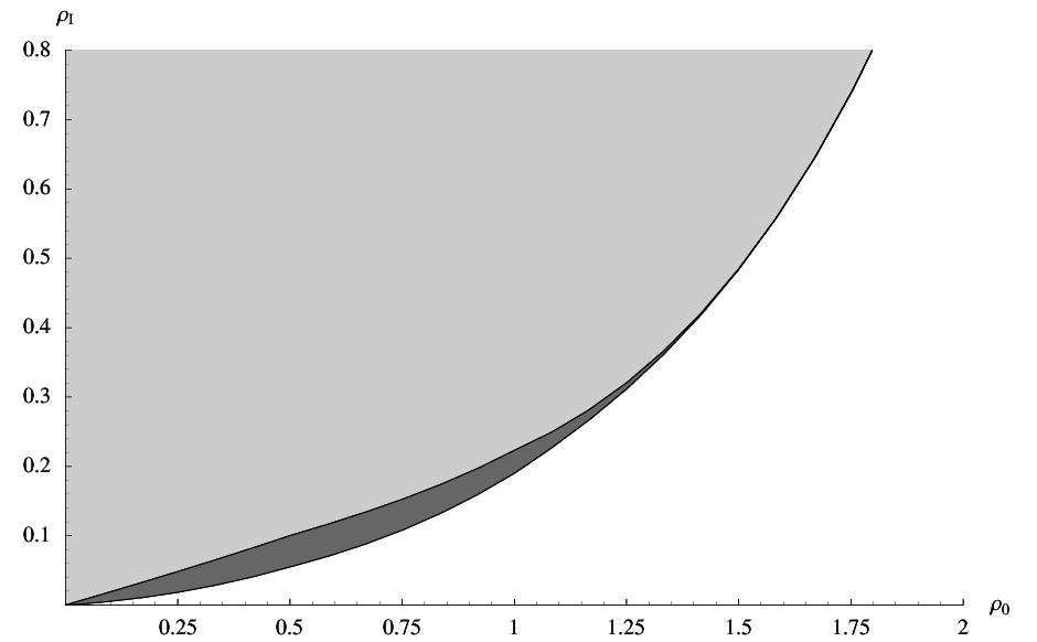
The singular and non-singular two-parameter families are separated by a one-parameter family that approaches $e^{2k}=e^{g+h}=N_{c}$ for $\rho\rightarrow\infty$. In fact, it asymptotically approaches the $\xi=2$ solution found in [10] and given above in equation (2.23). This one-parameter family will play a special role as discussed in the next subsection.
The analytic solutions discussed below comprise two-parameter families originating from Region I as long as they remain inside Regions I, II or III for all $\rho$ as well as a one-parameter family contained entirely in Region III. We will merely summarize these analytic solutions in this section and refer the interested reader to Appendix C for a detailed derivation.
Unfortunately, we were not able to find an analytic solution for the one-parameter family separating the two two-parameter families. We will therefore have to study them numerically in the next subsection. ¹²¹² 12 One particular solution of the one-parameter family of solutions ending at the point $e^{2k}=e^{g+h}=N_{c}$ and coming from the overlap of Region I and II was already found in Appendix D of [10].

The Solution Contained in Region I
For $e^{2k}\ll N_{c}$ we can solve the BPS equations (3.4) to first order in $e^{2k}$. The solution is

	$\displaystyle e^{g+h}/N_{c}$	$\displaystyle=$	$\displaystyle\rho_{0}-\rho+\frac{1}{64{\rho_{0}}^{2}{\rho_{I}}^{2}}\left(\frac{1}{4}\left(1+8(\rho-\rho_{0})^{2}\sinh{4\rho}\right)\right.$		(3.9)
			$\displaystyle-\left.(\rho-\rho_{0})\cosh{4\rho}-\rho_{0}+\frac{8}{3}\rho(\rho^{2}-3\rho\rho_{0}+3\rho_{0}^{2})\right),$
	$\displaystyle e^{2k}/N_{c}$	$\displaystyle=$	$\displaystyle\left(\frac{\sinh{2\rho}}{2\rho_{I}}\left(1-\frac{\rho}{\rho_{0}}\right)\right)^{2}.$		(3.10)

For this solution to be entirely contained in Region I we need to impose $e^{2k}\ll N_{c}$ for all $\rho$. Note that this solution does not only have a singularity at $\rho=0$ but also a second one near $\rho=\rho_{0}$. At the singularity at $\rho=0$ the dilaton and the metric component $g_{tt}$ both go to a constant. On the other hand both go to infinity at the other singularity. It is not clear whether these solutions can be given a physical interpretation.

The Solution Starting in Region II and Ending in Region III
For a somewhat limited choice of initial conditions, meaning $\rho_{0}\gg 1$ and $\rho_{I}\ll 1$ or $\rho_{0},\rho_{I}\gg 1$, we can find a closed form for the analytic solution approximating the solution starting in the overlap of Region I and II and ending in Region III. For $\rho_{I}\ll 1$ and $\rho_{0}\gg 1$ we find

	$\displaystyle e^{g+h}/N_{c}$	$\displaystyle=$	$\displaystyle\rho_{0}\left(1-\frac{1}{8\rho_{0}{\rho_{I}}^{2}}\left(3\rho-\frac{3}{4}\sinh{4\rho}\right)\right)^{\frac{1}{3}},$		(3.11)
	$\displaystyle e^{2k}/N_{c}$	$\displaystyle=$	$\displaystyle\left(\frac{\sinh{2\rho}}{2\rho_{I}}\right)^{2}\left(1-\frac{1}{8\rho_{0}{\rho_{I}}^{2}}\left(3\rho-\frac{3}{4}\sinh{4\rho}\right)\right)^{-\frac{2}{3}},$		(3.12)

while for $\frac{1}{4}e^{2\rho_{0}}\gg\rho_{I}\gg 1$ and $\rho_{0}\gg 1$ the solution is

	$\displaystyle e^{g+h}/N_{c}$	$\displaystyle=$	$\displaystyle\rho_{0}\left(1+\frac{3e^{4\rho}}{64\rho_{0}{\rho_{I}}^{2}}\right)^{\frac{1}{3}}-\rho,$		(3.13)
	$\displaystyle e^{2k}/N_{c}$	$\displaystyle=$	$\displaystyle\left(\frac{\sinh{2\rho}}{2\rho_{I}}\right)^{2}\left(1+\frac{3e^{4\rho}}{64\rho_{0}{\rho_{I}}^{2}}\right)^{-\frac{2}{3}}.$		(3.14)

As discussed below, we think that these solutions describe the geometry generated by the color and flavor D5-branes. For somewhat less restrictive initial conditions the matching can still be done but with piecewise defined functions that give a slightly better approximation to the numerical results. This is described in more detail in Appendix C.

The Solution Contained in Region III
Solving the equations for $e^{2k}\gg N_{c}$ by neglecting $N_{c}$ in the BPS equations (3.4) one finds

	$\displaystyle e^{g+h}/N_{c}$	$\displaystyle=$	$\displaystyle A\left(8B-12\rho+3\sinh{4\rho}\right)^{\frac{1}{3}},$		(3.15)
	$\displaystyle e^{2k}/N_{c}$	$\displaystyle=$	$\displaystyle\frac{8A\sinh^{2}{2\rho}}{(8B-12\rho+3\sinh{4\rho})^{\frac{2}{3}}}.$		(3.16)

For this solution to be entirely contained in Region III we need to demand that $e^{2k}\gg N_{c}$ for all $\rho$. In particular this has to hold in the limit $\rho\rightarrow 0$ which implies $B=0$. After making the identification $A=\frac{\epsilon^{\frac{4}{3}}}{2^{\frac{4}{3}}3^{\frac{1}{3}}}$ this solution can be seen to correspond to the deformed conifold [29]

	$\displaystyle e^{g+h}/N_{c}$	$\displaystyle=$	$\displaystyle\frac{\epsilon^{\frac{4}{3}}\left(\sinh{4\rho}-4\rho\right)^{\frac{1}{3}}}{2^{\frac{4}{3}}},$		(3.17)
	$\displaystyle e^{2k}/N_{c}$	$\displaystyle=$	$\displaystyle\frac{2}{3}\epsilon^{\frac{4}{3}}\frac{2^{\frac{2}{3}}\sinh^{2}{2\rho}}{(\sinh{4\rho}-4\rho)^{\frac{2}{3}}}.$		(3.18)

In order for it to be contained entirely in Region III we require $\epsilon\gg\left(\frac{3}{2}\right)^{\frac{1}{4}}\approx 1$.

The two-parameter families of solutions reaching the point $e^{2k}=e^{g+h}=0$ for finite $\rho=\rho_{s}$ are singular both at $\rho=0$ as well as at $\rho=\rho_{s}$. The Ricci scalar close to the singularities scales as $1/\rho^{2}$ and $1/(\rho-\rho_{s})^{2}$, respectively. We do not know whether these solutions are physical.
For the two-parameter family of solutions which approaches $e^{2k}=\frac{4}{3}e^{g+h}-\frac{N_{c}}{2}$ as $\rho\rightarrow\infty$ we can write the metric for large $\rho$ as

$$ds^{2}=\alpha^{\prime}g_{s}N_{c}\,e^{\phi(r)/2}\left(\frac{dx_{1,3}^{2}}{\alpha^{\prime}g_{s}N_{c}}+dr^{2}+r^{2}ds^{2}_{T_{11}}\right),$$

(3.19)

where we defined a new radial coordinate $r\sim e^{2\rho/3}$ and $ds^{2}_{T_{11}}$ is the Einstein metric on the homogeneous space $(SU(2)\times SU(2))/U(1)_{\text{diag}}$. So for large values of the radial coordinate the metric approaches a product of Minkowski space and the singular conifold. As $\rho$ goes to zero the geometry is singular and the Ricci scalar diverges like $1/\rho^{2}$. This should be compared to the usual $1/\rho$ divergence for flat D5-branes. We attribute the discrepancy to the way the flavor branes are embedded. According to the criteria developed in [30] the solutions should still be accepted as being physical since the $g_{tt}$ component of the metric remains bounded as $\rho$ approaches zero. The dilaton increases monotonically with $\rho$ and for large values of $\rho$ approaches a constant. So as long as $g_{s}N_{c}\gg 1$ the Ricci scalar is small for all large enough $\rho$, and, if $g_{s}\ll 1$ as well, this means that the supergravity approximation is valid. We believe that these solutions describe the geometry generated by the $N_{c}$ color branes in the presence of $N_{f}=2N_{c}$ smeared flavor branes.
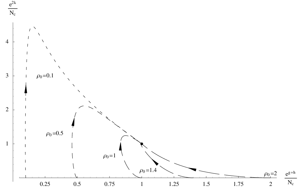
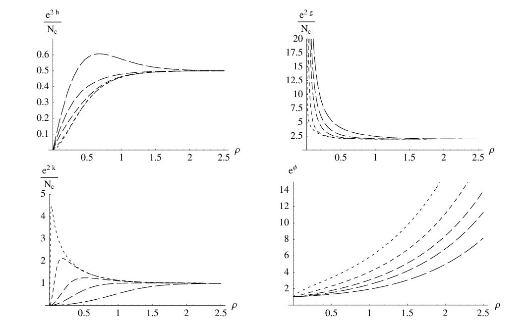
These two two-parameter families are separated by a one-parameter family that approaches $e^{2k}=e^{g+h}=N_{c}$ for $\rho\rightarrow\infty$. This situation of having two classes of solutions separated by ‘special’ solutions should be familiar from e.g. the Klebanov-Tseytlin solution [31]. There one has an integration constant $b_{0}$. For $b_{0}<0$ one finds solutions that have a second singularity for finite value of the radial coordinate. For $b_{0}>0$ the solutions describe the geometries generated by the brane configuration. For $b_{0}=0$ one obtains special solutions describing the corresponding near horizon geometries. Before fixing the boundary conditions at infinity a similar behavior can be observed for a stack of Dp-branes in flat space. This leads us to the conclusion that our one-parameter family separating the singular and non-singular two-parameter families describes the near horizon geometry for our brane setup and should be dual to $\mathcal{N}=1$ SQCD with $N_{f}=2N_{c}$. Due to the singularity at $\rho=0$ we should impose an IR cut-off. There also has to be a UV cut-off due to the presence of Kaluza-Klein modes. These become important as the energy increases. At even higher energies the theory becomes six dimensional and has a little string theory as its UV completion. We should note that it is not clear that the IR and UV cut-off are even compatible (in the sense that all approximations are valid) but we find that at least for a certain range of initial conditions this is the case. In the next section we study Wilson loops and beta functions for these solutions to support our interpretation. Unfortunately, we do not have an analytic expression describing these geometries because the near horizon limit takes us out of the regime where our approximations (3.2) are valid. So we study these solutions numerically. Figure 3 shows a few examples of this one-parameter family of solutions.

As usual the Wilson loop for two non-dynamical quarks can be computed by evaluating the Nambu-Goto action of a fundamental string with appropriate boundary conditions on shell [32],[33]. We will parametrize the string world sheet by $t=\tau$, $x=\sigma$ and $\rho=\rho(\sigma)$. Suppose we study a quark and an antiquark separated by a distance $L$ along the $x$-direction in gauge theory coordinates. The energy and length of the string can be given as functions of $\rho$, where $\rho$ is the minimal coordinate distance between the worldsheet and the singularity. In the string frame these become

	$\displaystyle L(\rho)$	$\displaystyle=2\sqrt{\alpha^{\prime}g_{s}}\int_{\rho}^{\overline{\rho}}e^{k(\rho^{\prime})}\frac{e^{\phi(\rho)}}{\sqrt{e^{2\phi(\rho^{\prime})}-e^{2\phi(\rho)}}}d\rho^{\prime},$		(4.1)
	$\displaystyle E(\rho)$	$\displaystyle=\frac{\sqrt{g_{s}}}{2\pi\sqrt{\alpha^{\prime}}}\left(2\int_{\rho}^{\overline{\rho}}\frac{e^{2\phi(\rho^{\prime})+k(\rho^{\prime})}}{\sqrt{e^{2\phi(\rho^{\prime})}-e^{2\phi(\rho)}}}d\rho^{\prime}-2\int_{0}^{\overline{\rho}}e^{\phi(\rho^{\prime})+k(\rho^{\prime})}d\rho^{\prime}\right),$		(4.2)

where $\overline{\rho}$ is a cutoff that can be taken to infinity at the end of the calculation. We will study these integrals numerically and must work with a large but finite cut-off. We have checked that the cut-off is large enough to make our results cut-off independent. The results can be used to obtain a relation $E(L)\equiv V_{q\bar{q}}(L)$. We will calculate the Wilson loops for the same set of parameters as shown in Figure 3 above. For solutions with $\rho_{0}<\rho_{c}\sim 1.6$ we find that $L(\rho)$ has a maximum at $\rho$ comparable to the value of $\rho$ for which the supergravity approximation breaks down. This is shown in Figures 4 and 5. For $\rho_{0}>\rho_{c}\sim 1.6$ $L(\rho)$ approaches $\sqrt{\alpha^{\prime}g_{s}N_{c}}\pi$ from below.¹³¹³ 13 Using the large $\rho$ behavior of our solutions, namely that $e^{2k}\rightarrow N_{c}$ and $e^{\phi}\rightarrow e^{\phi_{0}+\rho}$, it is straightforward to check that for large $\rho$ we have $L(\rho)\sim 2\sqrt{\alpha^{\prime}g_{s}N_{c}}\int_{0}^{\infty}\frac{d\rho^{\prime}}{\sqrt{e^{2\rho^{\prime}}-1}}=\pi\sqrt{\alpha^{\prime}g_{s}N_{c}}$ .

References

- [1] J. M. Maldacena, “The large N limit of superconformal field theories and supergravity,” Adv. Theor. Math. Phys. 2, 231 (1998) [Int. J. Theor. Phys. 38, 1113 (1999)] [arXiv:hep-th/9711200].
- [2] E. Witten, “Anti-de Sitter space and holography,” Adv. Theor. Math. Phys. 2, 253 (1998) [arXiv:hep-th/9802150].
- [3] O. Aharony, S. S. Gubser, J. M. Maldacena, H. Ooguri and Y. Oz, “Large N field theories, string theory and gravity,” Phys. Rept. 323, 183 (2000) [arXiv:hep-th/9905111].
- [4] A. H. Chamseddine and M. S. Volkov, “Non-Abelian BPS monopoles in N = 4 gauged supergravity,” Phys. Rev. Lett. 79, 3343 (1997) [arXiv:hep-th/9707176].
- [5] A. H. Chamseddine and M. S. Volkov, “Non-Abelian solitons in N = 4 gauged supergravity and leading order string theory,” Phys. Rev. D 57, 6242 (1998) [arXiv:hep-th/9711181].
- [6] J. M. Maldacena and C. Nunez, “Towards the large N limit of pure N = 1 super Yang Mills,” Phys. Rev. Lett. 86, 588 (2001) [arXiv:hep-th/0008001].
- [7] I. R. Klebanov and M. J. Strassler, “Supergravity and a confining gauge theory: Duality cascades and chiSB-resolution of naked singularities,” JHEP 0008, 052 (2000) [arXiv:hep-th/0007191].
- [8] A. Karch and E. Katz, “Adding flavor to AdS/CFT,” JHEP 0206, 043 (2002) [arXiv:hep-th/0205236].
- [9] M. Kruczenski, D. Mateos, R. C. Myers and D. J. Winters, JHEP 0307, 049 (2003) [arXiv:hep-th/0304032]. M. Kruczenski, D. Mateos, R. C. Myers and D. J. Winters, JHEP 0405, 041 (2004) [arXiv:hep-th/0311270]. J. Babington, J. Erdmenger, N. J. Evans, Z. Guralnik and I. Kirsch, Phys. Rev. D 69, 066007 (2004) [arXiv:hep-th/0306018]. D. Mateos, R. C. Myers and R. M. Thomson, Phys. Rev. Lett. 97, 091601 (2006) [arXiv:hep-th/0605046]. T. Albash, V. G. Filev, C. V. Johnson and A. Kundu, arXiv:hep-th/0605088. T. Sakai and S. Sugimoto, Prog. Theor. Phys. 113, 843 (2005) [arXiv:hep-th/0412141].
- [10] R. Casero, C. Nunez and A. Paredes, “Towards the string dual of N = 1 SQCD-like theories,” Phys. Rev. D 73, 086005 (2006) [arXiv:hep-th/0602027].
- [11] F. Benini, F. Canoura, S. Cremonesi, C. Nunez and A. V. Ramallo, “Unquenched flavors in the Klebanov-Witten model,” JHEP 0702, 090 (2007) [arXiv:hep-th/0612118].
- [12] F. Benini, F. Canoura, S. Cremonesi, C. Nunez and A. V. Ramallo, “Backreacting Flavors in the Klebanov-Strassler Background,” arXiv:0706.1238 [hep-th].
- [13] C. Nunez, A. Paredes and A. V. Ramallo, “Flavoring the gravity dual of N = 1 Yang-Mills with probes,” JHEP 0312, 024 (2003) [arXiv:hep-th/0311201].
- [14] G. Papadopoulos and A. A. Tseytlin, “Complex geometry of conifolds and 5-brane wrapped on 2-sphere,” Class. Quant. Grav. 18, 1333 (2001) [arXiv:hep-th/0012034].
- [15] S. S. Gubser, A. A. Tseytlin and M. S. Volkov, “Non-Abelian 4-d black holes, wrapped 5-branes, and their dual descriptions,” JHEP 0109, 017 (2001) [arXiv:hep-th/0108205].
- [16] N. Seiberg, “New theories in six dimensions and matrix description of M-theory on T**5 and T**5/Z(2),” Phys. Lett. B 408, 98 (1997) [arXiv:hep-th/9705221].
- [17] A. Losev, G. W. Moore and S. L. Shatashvili, “M & m’s,” Nucl. Phys. B 522, 105 (1998) [arXiv:hep-th/9707250].
- [18] O. Aharony, “A brief review of ’little string theories’,” Class. Quant. Grav. 17, 929 (2000) [arXiv:hep-th/9911147].
- [19] N. Itzhaki, J. M. Maldacena, J. Sonnenschein and S. Yankielowicz, “Supergravity and the large N limit of theories with sixteen supercharges,” Phys. Rev. D 58, 046004 (1998) [arXiv:hep-th/9802042].
- [20] J. P. Gauntlett, N. Kim, D. Martelli and D. Waldram, “Wrapped fivebranes and N = 2 super Yang-Mills theory,” Phys. Rev. D 64, 106008 (2001) [arXiv:hep-th/0106117].
- [21] M. Bershadsky, C. Vafa and V. Sadov, “D-Branes and Topological Field Theories,” Nucl. Phys. B 463, 420 (1996) [arXiv:hep-th/9511222].
- [22] S. S. Gubser, “Curvature singularities: The good, the bad, and the naked,” Adv. Theor. Math. Phys. 4, 679 (2002) [arXiv:hep-th/0002160].
- [23] R. Casero, C. Nunez and A. Paredes, “Elaborations on the String Dual to N=1 SQCD,” arXiv:0709.3421 [hep-th].
- [24] G. Bertoldi, F. Bigazzi, A. L. Cotrone and J. D. Edelstein, “Holography and Unquenched Quark-Gluon Plasmas,” arXiv:hep-th/0702225.
- [25] F. Bigazzi, R. Casero, A. L. Cotrone, E. Kiritsis and A. Paredes, “Non-critical holography and four-dimensional CFT’s with fundamentals,” JHEP 0510, 012 (2005) [arXiv:hep-th/0505140].
- [26] A. Karch and L. Randall, “Open and closed string interpretation of SUSY CFT’s on branes with boundaries,” JHEP 0106, 063 (2001) [arXiv:hep-th/0105132].
- [27] C. Bachas and M. Petropoulos, “Anti-de-Sitter D-branes,” JHEP 0102, 025 (2001) [arXiv:hep-th/0012234].
- [28] E. Bergshoeff, R. Kallosh, T. Ortin and G. Papadopoulos, “kappa-symmetry, supersymmetry and intersecting branes,” Nucl. Phys. B 502, 149 (1997) [arXiv:hep-th/9705040].
- [29] P. Candelas and X. C. de la Ossa, “Comments on Conifolds,” Nucl. Phys. B 342, 246 (1990).
- [30] J. M. Maldacena and C. Nunez, “Supergravity description of field theories on curved manifolds and a no go theorem,” Int. J. Mod. Phys. A 16, 822 (2001) [arXiv:hep-th/0007018].
- [31] I. R. Klebanov and A. A. Tseytlin, “Gravity duals of supersymmetric SU(N) x SU(N+M) gauge theories,” Nucl. Phys. B 578, 123 (2000) [arXiv:hep-th/0002159].
- [32] J. M. Maldacena, “Wilson loops in large N field theories,” Phys. Rev. Lett. 80, 4859 (1998) [arXiv:hep-th/9803002].
- [33] S. J. Rey and J. T. Yee, “Macroscopic strings as heavy quarks in large N gauge theory and anti-de Sitter supergravity,” Eur. Phys. J. C 22, 379 (2001) [arXiv:hep-th/9803001].
- [34] A. W. Peet and J. Polchinski, “UV/IR relations in AdS dynamics,” Phys. Rev. D 59, 065011 (1999) [arXiv:hep-th/9809022].
- [35] E. Caceres and C. Nunez, “Glueballs of super Yang-Mills from wrapped branes,” JHEP 0509, 027 (2005) [arXiv:hep-th/0506051].
- [36] G. Policastro, D. T. Son and A. O. Starinets, “The shear viscosity of strongly coupled N = 4 supersymmetric Yang-Mills plasma,” Phys. Rev. Lett. 87, 081601 (2001) [arXiv:hep-th/0104066].
- [37] G. Policastro, D. T. Son and A. O. Starinets, “From AdS/CFT correspondence to hydrodynamics,” JHEP 0209, 043 (2002) [arXiv:hep-th/0205052].
- [38] P. Kovtun, D. T. Son and A. O. Starinets, “Viscosity in strongly interacting quantum field theories from black hole physics,” Phys. Rev. Lett. 94, 111601 (2005) [arXiv:hep-th/0405231].
- [39] C. P. Herzog, A. Karch, P. Kovtun, C. Kozcaz and L. G. Yaffe, JHEP 0607, 013 (2006) [arXiv:hep-th/0605158]. S. S. Gubser, Phys. Rev. D 74, 126005 (2006) [arXiv:hep-th/0605182]. H. Liu, K. Rajagopal and U. A. Wiedemann, Phys. Rev. Lett. 98, 182301 (2007) [arXiv:hep-ph/0607062]. H. Liu, K. Rajagopal and U. A. Wiedemann, Phys. Rev. Lett. 97, 182301 (2006) [arXiv:hep-ph/0605178]. E. Caceres and A. Guijosa, JHEP 0612, 068 (2006) [arXiv:hep-th/0606134]. E. Caceres and A. Guijosa, JHEP 0611, 077 (2006) [arXiv:hep-th/0605235]. A. Buchel, Phys. Rev. D 74, 046006 (2006) [arXiv:hep-th/0605178]. E. Caceres, M. Natsuume and T. Okamura, JHEP 0610, 011 (2006) [arXiv:hep-th/0607233]. M. Chernicoff and A. Guijosa, JHEP 0702, 084 (2007) [arXiv:hep-th/0611155]. S. D. Avramis and K. Sfetsos, JHEP 0701, 065 (2007) [arXiv:hep-th/0606190]. J. Mas, JHEP 0603, 016 (2006) [arXiv:hep-th/0601144]. N. Armesto, J. D. Edelstein and J. Mas, JHEP 0609, 039 (2006) [arXiv:hep-ph/0606245]. S. D. Avramis, K. Sfetsos and D. Zoakos, Phys. Rev. D 75, 025009 (2007) [arXiv:hep-th/0609079]. M. Chernicoff, J. A. Garcia and A. Guijosa, JHEP 0609, 068 (2006) [arXiv:hep-th/0607089]. M. Natsuume and T. Okamura, JHEP 0709, 039 (2007) [arXiv:0706.0086 [hep-th]].
- [40] O. Aharony, E. Schreiber and J. Sonnenschein, JHEP 0204, 011 (2002) [arXiv:hep-th/0201224]. V. Borokhov and S. S. Gubser, JHEP 0305, 034 (2003) [arXiv:hep-th/0206098]. N. J. Evans, M. Petrini and A. Zaffaroni, JHEP 0206, 004 (2002) [arXiv:hep-th/0203203].
- [41] E. Bergshoeff and P. K. Townsend, “Super D-branes,” Nucl. Phys. B 490, 145 (1997) [arXiv:hep-th/9611173].
- [42] E. Bergshoeff and P. K. Townsend, “Super-D branes revisited,” Nucl. Phys. B 531, 226 (1998) [arXiv:hep-th/9804011].
- [43] J. H. Schwarz, “Covariant Field Equations Of Chiral N=2 D=10 Supergravity,” Nucl. Phys. B 226, 269 (1983).