Understanding Confinement From Deconfinement
Abstract
We use effective magnetic pure gauge theory with cutoff and fixed gauge coupling to calculate non-perturbative magnetic properties of the deconfined phase of Yang-Mills theory. We obtain the response to an external closed loop of electric current by reinterpreting and regulating the calculation of the one loop effective potential in Yang-Mills theory. This effective potential gives rise to a color magnetic charge density, the counterpart in the deconfined phase of color magnetic currents introduced in effective dual superconductor theories of the confined phase via magnetically charged Higgs fields. The resulting spatial Wilson loop has area law behavior. Using values of and determined in the confined phase, we find spatial string tensions compatible with lattice simulations in the temperature interval . Use of the effective theory to analyze experiments on heavy ion collisions will provide applications and further tests of these ideas.
1 Introduction
The confined phase of Yang-Mills theory can be described by an effective theory coupling magnetic gauge potentials to three adjoint representation Higgs fields [1]. The coupling of the potentials to the magnetically charged Higgs fields generate color magnetic currents which, via a dual Meissner effect, confine electric flux to narrow tubes connecting a quark-antiquark pair [2]. The dual gluon (quanta of the magnetic gauge theory) aquires a mass . For , [3]. The effective theory is applicable at distances greater than the flux tube radius . Since lattice simulations [4] yield a deconfinement temperature , the scale . There is then a range of temperatures within the interval where the effective theory should also be applicable in the deconfined phase. We will use the theory in this temperature range to calculate spatial Wilson loops, quantities that are outside the perturbative realm of finite temperature Yang-Mills theory.
In Section 2 we review the use of the effective theory in the confined phase. In Section 3 we point out that in the deconfined phase the Higgs fields, in contrast to the gauge potentials, do not form part of the massless sector of the theory. We neglect them at temperatures not too close to , so that the effective theory reduces to magnetic Yang-Mills theory with a cutoff and gauge coupling constant fixed by fits of heavy quark potentials in the confined phase [3].
In section 4 we show that the spatial Wilson loop of Yang-Mills theory is determined by the effective potential of the magnetic theory in the background of a static dual scalar potential . We evaluate the one loop contribution to , and use it to calculate the spatial string tensions that measure the magnetic flux with quantum number passing through a large loop. We find that these string tensions are proportional to (Casimir scaling), and that the predicted string tension is compatible with the results of lattice simulations [5] in the temperature range .
In section 5 we compare lattice simulations of string tensions with lattice simulations [6] of dual string tensions (measuring electric flux) in the temperature range . We find that the temperature marks a ”transition” from a high temperature perturbative regime having to a low temperature domain where .
In section 6 we compare the spatial string tension, calculated in the effective magnetic gauge theory, with that calculated [7] in the large , large ’t Hooft coupling limit of super Yang-Mills theory.
In the final section we summarize the results, discuss the significance of this work and suggest extensions and further tests.
2 Effective Theory of the Confined Phase
The effective theory describing the low energy excitations of SU(N) Yang-Mills theory is a long distance dual Yang-Mills theory coupling non-Abelian magnetic SU(N) gauge potentials to 3 scalar fields , each in the adjoint representation of the magnetic gauge group. The Lagrangian has the form [1]
| (1) |
where
| (2) |
and
| (3) |
is a Higgs potential which has a minimum at nonzero values of . It is chosen so that the Lagrangian (1) describes a dual superconductor on the border between type I and type II.
In the confined phase the magnetic gauge symmetry is completely broken via a dual Higgs mechanism in which all particles become massive. (At least adjoint scalars are necessary to completely break the symmetry.) The value of the magnetic Higgs condensate is determined by the location of the minimum in the Higgs potential, and the dual (magnetic) gluon acquires a mass
| (4) |
via the dual Higgs mechanism.
The simplest possibility for the vacuum condensate has the color structure [1].
| (5) |
where , , and are the three generators of the N dimensional irreducible representation of the three dimensional rotation group corresponding to angular momentum . Since any matrix which commutes with all three generators must be a multiple of the unit matrix, there is no transformation which leaves all three invariant and the dual gauge symmetry is completely broken.
The excitations above the classical vacuum of the effective theory are flux tubes connecting a quark-antiquark pair in which electric flux is confined to narrow tubes of radius , at whose center the Higgs condensate vanishes. Explicit solutions have been obtained for . The scale of the energy distribution in these electric flux tubes is determined by the dual gluon mass . Since the effective theory describes fluctuations only at energy scales less than , there is no physical excitation with this mass.
The effective theory has two parameters; and . Their values, and , were determined [3] by comparing the predicted static heavy quark potential with lattice simulations. For distances the lattice potential is well represented by the sum of a term linear in and a term, [8]. The value of is obtained by writing the lattice potential in an effective Coulomb form:
| (6) |
The RHS of (6) is the potential obtained by coupling magnetic gluons to a Dirac string connecting a quark-antiquark pair with a strength , which is the perturbative result of the effective theory. The coefficient of the linear potential is proportional to and determines the value of in terms of and .
The spin dependent and velocity dependent heavy quark potentials calculated with the above values of and [3] are compatible with results obtained from lattice simulations [9]. Furthermore, predicted energy distributions in electric flux tubes are compatible with lattice results for these distributions for values of ranging from down to [10].
The long wavelength fluctuations of the axis of the electric flux tubes give rise to an effective bosonic string theory governed by the Nambu-Goto action [11]. These fluctuations are the low energy excitations of the effective theory. The value of obtained from (6) includes the energy, , of the long wave length oscillations of the axis of the flux tube [12]. The value of is close to , so that the main contribution to comes from renormalization due to string fluctuations. Short distance fluctuations at energy scales greater than do not enter in the effective theory, and is the coupling constant defined at the fixed scale .
3 The Effective Theory in the Deconfined Phase
An approximate one loop calculation [13] of a finite temperature effective potential for the Higgs fields yielded a potential whose minimum moved to at a temperature . The deconfinement temperature is then on the order of . Above the Higgs condensate vanishes, so the magnetic gluon becomes massless. However, since the deconfinement temperature for groups with is first order [4, 14], the Higgs particles remain massive in the deconfined phase. (This first order phase transition was not seen in the calculation [13] since it did not include the contribution of a cubic term in the Higgs potential.)
Since above the Higgs fields do not form part of the massless spectrum, we will neglect them in our treatment of the deconfined phase. Then in the leading long distance approximation the effective theory reduces to a pure SU(N) Yang-Mills theory of magnetic gauge potentials . Although inclusion of the Higgs fields is essential in order to describe the transition to the confined phase, we will see a signal for this transition in the behavior of the pure gauge effective theory as the temperature is lowered toward .
This theory has the same form as the microscopic electric theory, but with a fixed gauge coupling constant and fixed ultraviolet cutoff . The values of these two parameters are determined by the effective theory description of the confined phase. The magnetic gluons, which at confine electric flux, become the physical degrees of freedom of the effective theory at . These quanta are ”strongly” interacting (), but their interaction is cut off at distances less than . Because of the duality between the microscopic electric Yang-Mills theory and the effective long distance magnetic gauge theory, perturbative calculations of electric quantities in the microscopic theory can be adapted to calculate magnetic quantities in the effective theory.
4 The Spatial Wilson Loop Calculated in the Magnetic Theory.
To test the idea of using the effective theory to calculate magnetic quantities in the deconfined phase we calculate spatial Wilson loops measuring magnetic flux with quantum number passing through a loop . (The spatial Wilson loop has area law behavior both above and below .) The temporal Wilson loop of Yang-Mills theory determining the static heavy quark potential is the partition function of the effective dual theory in the presence of a Dirac string connecting a static quark-antiquark pair [1]. Similarly the spatial Wilson loop is the partition function of the effective dual theory in the presence of a current of quarks circulating around the loop ( closed Dirac strings). This current is the source of a color magnetic field , the magnetic analogue of the color electric field generated in the confined phase by the Dirac string [1] :
| (7) |
The operator creating the closed Dirac string is a singular dual gauge transformation which changes by a factor when it encircles a curve linking the loop . It is the dual of the spatial ’t Hooft loop operator that creates a closed line of magnetic flux along a loop in Yang-Mills theory [15, 16]. The effect of the dual ’t Hooft operator is to add to an external potential which is the magnetostatic scalar potential produced by circulating quark loops, each carrying a steady current and one unit of charge. (The total color charge transported along the Dirac string is and the total elapsed Euclidean time is .)
The th circulating quark gives a contribution to proportional to a diagonal matrix whose th diagonal element is equal to and whose remaining elements are equal to . The sum over the quarks gives [17]
| (8) |
where is the solid angle subtended at the point by a surface bounded by the loop , and where is a diagonal matrix having its first elements equal to and its remaining elements equal to . (The matrix reflects the charge carried by the circulating quark loops.) The gradient of contains a term (a magnetic shell) localized on the surface defining which is cancelled by a corresponding term in the action. The regular part of gives the Biot-Savart magnetic field of the current loop:
| (9) |
The spatial Wilson loop calculated in the dual theory is the partition function of the effective theory with replaced by , divided by the partition function with . Because is singular on , the functional integration defining is restricted to those configurations which vanish on the loop. (This boundary condition eliminates the singular cross term in the classical contribution to the action.)
4.1 The Effective Potential
To evaluate the partition function of the effective theory in the deconfined phase, where there is no classical potential, requires calculating the one loop effective potential in the background of a static magnetic scalar potential :
| (10) |
We have calculated integrating over the massless gauge modes of the magnetic theory and introducing a Pauli-Villars regulator mass to account for the short distance cutoff of the dual theory. This regulator mass should then be approximately equal to the dual gluon mass determining the maximum energy of the modes included in the effective theory. The calculation of , aside from the presence of the regulator, mimics the calculation of the one loop effective potential in Yang-Mills theory [18, 19] used to evaluate the spatial ’t Hooft loop [19, 20] . We assume that the background potential has the same color structure as , i.e., . The corresponding effective potential is a periodic function of with period , having minima at the inequivalent vacua of the magnetic theory.
The result for the 1-loop effective action is
| (11) |
where
| (12) |
and
| (13) |
with . The factor is the number of non zero eigenvalues of the matrix in the adjoint representation [17, 21]. The integral reflects the presence of the Pauli-Villars regulator in the functional determinant (10), which suppresses the short distance contribution to . The one loop effective potential is ultraviolet finite, so that in the absence of a regulator (), . In this limit the one loop effective potential (12), with replaced by and replaced by the running Yang-Mills coupling constant , reduces to .
The one loop expression for is applicable only at high temperatures where so that the contribution of higher order loops are small. The effective theory, by contrast, contains only modes having energies less than the mass scale . We will see that, for temperatures greater than , the one loop effective potential generates a classical solution having a mass scale greater than . Consequently, in the long distance effective theory, higher order corrections in the loop expansion about the classical solution can be neglected. We can then use the one loop effective potential to calculate Wilson loops via the effective theory (even though the coupling constant is not small).
Replacing by in (11) to account for the coupling to the Dirac string and adding the classical action gives the effective action, :
| (14) |
The background field is subject to the conditions for on , and as . The latter condition means that that the total magnetic field is short range, decaying to its vacuum value at large distances from the loop. , the minimum value of , determines the spatial Wilson loop, , as calculated in the effective theory.
The term in (14) linear in is a surface term which gives no contribution to because vanishes on . The term quadratic in (the magnetic energy of a current loop of a thin wire) is proportional to with a coefficient which diverges logarithmically as the thickness of the wire goes to zero. This ultraviolet divergence can be absorbed into a renormalization of the energy of the current source, after which the first term in (14) becomes simply and only the second term in (14) contains the external potential explicitly.
Because of the periodicity property of the effective potential, , the value of is independent of the choice of the surface defining the solid angle , and we can choose to be the plane surface bounded the loop . For a square loop of side in the plane centered at the origin
| (15) |
Since and , in minimizing (14) we can consider configurations which are odd functions of so that at for all and and the boundary condition on the loop is then automatically satisfied.

4.2 The Magnetic Energy Density Profile
The minimization of yields ”Poisson’s equation” for :
| (16) |
where
| (17) |
is the color magnetic charge density induced in the vacuum by the current loop. This charge produces a field screening , so that the total field has an exponential falloff determined by the dual screening mass :
| (18) |
Using Eqs.(12), (13) and (18), in Fig. 1 we plot as a function of for . Note that for , , and that as the temperature is lowered toward the screening mass , generated from the fluctuations of the massless quanta of the effective theory in the deconfined phase, decreases toward a value close to .

The dual screening mass determines the width of the magnetic energy profile surrounding a large spatial Wilson loop in the deconfined phase. To find this profile we first take the limit in (16) and (17). In this limit and are functions only of the distance from the loop. Furthermore the solid angle for and for , so that the boundary condition at large distances becomes as .
In Fig. 2 we plot at , obtained by solving (16) with these boundary conditions. Since for the mass , which determines the scale of the classical solution , is greater than the cutoff of the effective theory, then (as pointed out in Sec. (4.1)) higher loop corrections to the one loop effective potential can be neglected. In other words, there are no small scale fluctuations present in the effective theory to disturb the large scale structure of the classical solution, and the one loop profile function is self-consistent.
However, as is lowered to temperatures below , where the width of the magnetic energy profile becomes larger than the minimum wavelength of the fluctuations included in the effective theory, the classical energy distribution is destabilized and the one loop approximation breaks down. The breakdown of the pure gauge effective theory at lower temperatures is a signal for the transition to the confined phase for which the Higgs fields play an essential role.
4.3 Spatial String Tension: Comparison with Lattice Simulations
For large the effective action of the dual theory has area law behavior determining the spatial string tension :
| (19) |
Equivalently, the spatial string tension is the interface energy separating two vacua of magnetic gauge theory differing by units of charge [6].
The calculation of the spatial string tension follows closely the corresponding calculation of the dual spatial string tension , the interface energy in Yang-Mills theory [19, 20]. The one loop effective action evaluated at the ”classical” solution yields:
| (20) |
where
| (21) |
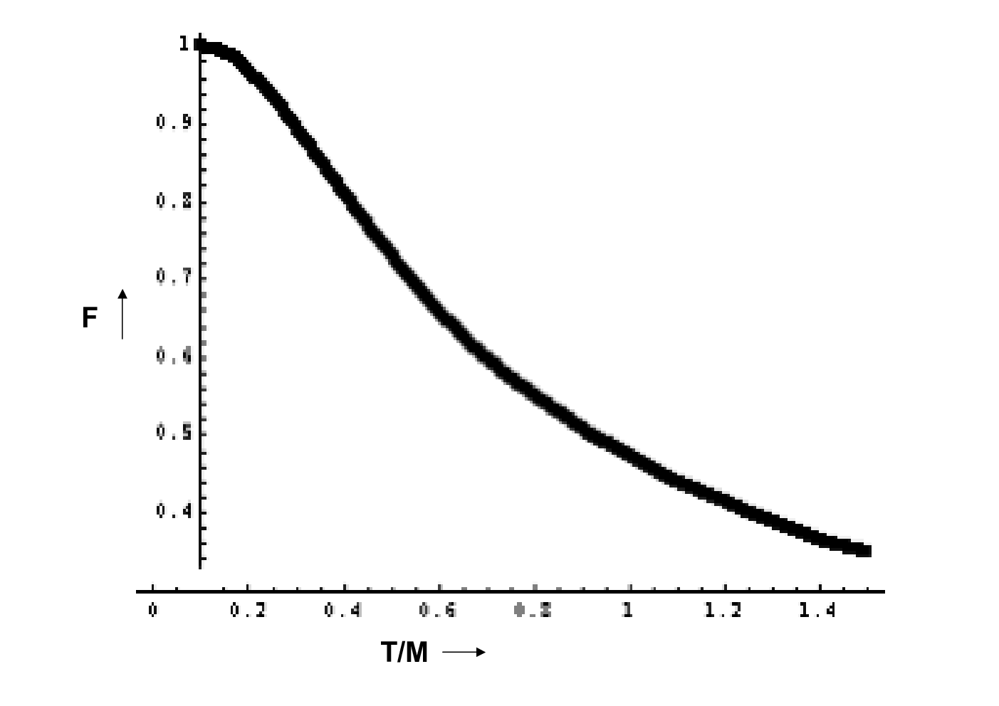
Eq.(20) is applicable for any group, but the values of and have been determined only for where the effective theory has been applied in the confined phase. The function , plotted in Fig. 3, is the ratio of the action with regulator mass to the unregulated action. The temperature dependence of the ratio comes from the Pauli-Villars cutoff, which suppresses the contributions of momenta greater than to . Since the Pauli-Villars regulator is rather ”soft”, allowing substantial contributions from momenta greater than , we have also evaluated the string tension using values of smaller than .

In Fig. 4 we plot for () as a function of for Paul-Villars masses , and , and compare with the results of 4d lattice simulations [5, 22]. We note the following features of these curves:
- •
At the predicted values of lie close to the lattice result, and they increase as the temperature increases, reflecting the decrease with temperature of the function (21) due to the Pauli-Villars regulator.
- •
gives the best fit to the lattice data in the temperature interval where the effective theory should be applicable.
- •
The value of the string tension does not depend strongly on the Pauli-Villars mass. (This reflects the ultra-violet finiteness of the one loop effective potential.)
- •
The lattice data in Fig. (4) are fit very well almost down to by combining the non-perturbative value of the string tension of 3d Yang-Mills theory (determining the high temperature limit of the 4d string tension) with the 2-loop calulation of the running of the coupling constant of 3d EQCD determining the change in the spatial string tension as the temperature is lowered) [22]. By contrast, the effective dual theory determines the string tension in the deconfined phase only in a limited temperature range, but uses parameters already determined in the confined phase. The values of the intercepts of the curves in Fig. (4), which are determined primarily by the value , are predictions of the effective theory. For example, for and , Eq. (20) with gives , while lattice simulations close to [14] give .
4.4 Spatial String Tension : Casimir Scaling
We note from (20) that is proportional to (Casimir scaling). This dependence on the quantum number of spatial string tensions in the deconfined phase is consistent with the results of lattice simulations of , , and gauge theories [14, 17]. Casimir scaling of the spatial string tension has also been obtained in a model of the deconfined phase as a gas of non-abelian monopoles in the adjoint representation [17, 21].
On the other hand such approximate Casimir scaling for the string tension would not be expected from the point of view of the effective theory because of the presence of the Higgs condensate in the confined phase.

4.5 Spatial String Tensions and Dual String Tensions Compared
In Fig. 5 we compare the lattice data for the string tension with data for dual string tensions measured in lattice simulations of , , and gauge theory in the temperature range [6]. The lattice data for for all these groups and for all possible values of k, when scaled by the Casimir factor , all collapse on a single curve shown by the large dots in Fig. 5 . This approximate Casimir scaling of dual string tensions agrees with the two loop perturbative prediction [17, 19]. At the magnitude of the dual string tension agrees with the two loop perturbative prediction, but at lower temperatures it is suppressed [6] relative to the perturbative prediction.
This temperature range, where non-perturbative effects on dual string tensions becomes significant, closely corresponds to the temperature range where the spatial string tension becomes comparable to the dual string tension. To show this, in Fig. 5 we also plot , using the string tension lattice data in Fig. 4. We see that at the string tension and that, as the temperature decreases, increases, becoming greater than for temperatures less than .
We can then identify three temperature intervals in the deconfined phase, each having distinctly different electric and magnetic responses according to the value of the ratio :
| (22) |
- •
, : The dual string tension is perturbatively calculable, and the effective magnetic theory can not be used to calculate the string tension ().
- •
, : The dual string tension is suppressed relative to its perturbative value, and the spatial string tension is calculable via the effective magnetic theory. ().
- •
, : Neither perturbation theory nor the effective magnetic theory are applicable. In this temperature range , which is a signal for the transition to the confined phase.
4.6 Spatial String Tension: Comparision with Super Yang-Mills Theory
In this section we compare the string tension predicted by the effective magnetic theory with the expression for the spatial string tension of super Yang-Mills theory, calculated in the large limit and in the limit of large ’t Hooft coupling , where the gravity-conformal field theory correspondence is applicable [7]:
| (23) |
There is no scale in SYM theory, is a free parameter, and the theory remains in the deconfined phase at all temperatures with .
In the scale free limit, , the one loop result of the effective magnetic theory is also constant. In this limit and (20) becomes
| (24) |
where
| (25) |
is the ’t Hooft coupling of the effective magnetic theory. Eq. (24) is applicable for any , but the value of is known only for where gives .
The factor in (24), determining in magnetic Yang-Mills theory, is proportional to the width of the magnetic profile multiplied by the number of unit charges in the large limit. The factor in (23), determining , arises from the relation between the ’t Hooft coupling and the fundamental string scale via the AdS/CFT correspondence.
The limit of (24) gives the factorized form:
| (26) |
Since the string tensions and ((23) and (26)) have the same dependence on the ’t Hooft couplings of the two theories, the corresponding string tensions will be equal if these two constants are related by a numerical factor of order unity. That is, imposing the relation
| (27) |
between the coupling constants and of the two theories, we obtain the equality of the two string tensions:
| (28) |
That is, with the correspondence (27) the spatial string tension is equal to the interface tension of magnetic gauge theory calculated with the one loop effective potential. This correspondence provides a link between effective magnetic Yang-Mills theory and supersymmetric Yang-Mills theory.
5 Summary
We have used effective magnetic pure gauge theory in the one loop approximation to calculate spatial Wilson loops in the deconfined phase in analogy to the use of the dual effective theory in the classical approximation to describe the confined phase.
Calculating the one loop effective potential for with an ultraviolet cutoff , we find:
- •
At the width of the magnetic energy profile (Fig. 2) is approximately equal to the radius of the electric flux tube.
- •
In the temperature interval the predicted spatial string tension is compatible with lattice simulations (Fig. 4).
- •
In this temperature interval the values of the string tension and the dual string tension obtained from lattice simulations (Fig. 5) approach each other and become equal as the temperature is lowered to about . Roughly speaking, the temperature scale marks a ”transition” in the behavior of the deconfined phase; the high temperature domain is described by perturbative Yang-Mills theory and the low temperature interval by the effective magnetic gauge theory.
- •
For SU(N) groups with the string tensions satisfy Casimir scaling (while Casimir scaling is not expected in the confined phase).
- •
With the duality correspondence (27) the spatial string tension , calculated in SYM theory, is equal to string tension , calculated in the effective magnetic theory in the scale free limit.
6 Discussion
The formation of the magnetic energy profile around a spatial Wilson loop in the deconfined phase parallels formation of an electric flux tube in the confined phase.
In the confined phase an open Dirac string connecting a quark-antiquark pair couples to the magnetic vector potential and induces a magnetic color current density brought about by the interaction of the gauge potentials with the magnetically charged Higgs fields. Via the dual of Ampere’s law this current density gives rise to an electric field which screens the external Coulomb field generated by the open Dirac string, so that the total color electric field decays exponentially with the energy profile of an electric flux tube.
In the deconfined phase a closed Dirac string couples to the magnetic scalar potential and induces an effective magnetic color charge density generated by the one loop effective . Via the dual of Gauss’s law this magnetic charge density gives rise to a magnetic field which screens the external Biot-Savart magnetic field generated by the closed Dirac string, so that the total magnetic field decays exponentially at large distances and has the energy profile shown in Fig. 2.
We thus gain an understanding of confinement by studying the deconfined phase. The magnetic currents confining electric flux, introduced at the classical level via Higgs fields, are the counterparts in the confined phase of magnetic charges, generated in the deconfined phase by integrating out the long distance quantum fluctuations of the non-Abelian magnetic degrees of freedom. As the temperature is lowered toward the confined magnetic energy profile resulting from the one loop pure gauge effective action becomes unstable, signaling the transition to the confined phase. Here the inclusion in the effective action of the magnetically charged Higgs fields leads to topologically stable classical electric flux tube solutions.
According to our picture, the effective theory describing the deconfined phase in a temperature range included in the interval is Yang-Mills theory, just as in the microscopic theory. Only the physical interpretation of the potentials and the scale of the theory are altered. In the temperature interval the deconfined phase consists of magnetic charges composed of massless magnetic gluons, interacting ”strongly” () over distances greater than . Since this temperature interval is accessible in heavy ion collisions, calculations of non-equilibrium quantities in the effective theory would make it possible to test the picture of the deconfined phase as a strongly interacting system of magnetic gluons. Because of the presence of the long distance cutoff, it should be possible to adapt perturbation calculations, carried out in microscopic Yang-Mills theory and applicable only at high temperatures, to the calculation of corresponding properties in the effective magnetic Yang-Mills theory.
7 Further Tests and Investigations
- •
In the confined phase the long wavelength fluctuations of the axis of the flux tubes give rise to an effective bosonic string theory and consequently to the Lüscher correction to the area law behavior of Wilson loops. In contrast, in the deconfined phase there is no Higgs condensate whose zeros locate the position of the string, and conseqently no effective string theory. Instead, in order to calculate the corrections to the area law behavior of spatial Wilson loops in the deconfined phase in the temperature range where the effective theory is applicable we must solve (16) for finite values of and evaluate the corresponding effective action (14). This calculation will be described in a separate paper.
- •
Evidence for the magnetic quanta of the effective theory should be sought in lattice simulations of Yang-Mills theory in the deconfined phase.
- •
The effective magnetic Yang-Mills theory should be used to analyze experiments on heavy ion collisions.
Acknowledgments
I would like to thank O. Aharony, B. Bringoltz, Ph. de Forcrand, M. Fromm, A. Karch, C. P. Korthals Altes, A. Vuorinen and L. Yaffe for their valuable help.
References
- [1] M. Baker, J. S. Ball and F. Zachariasen, Phys. Rev. D 44, 3328 (1991).
- [2] S. Mandelstam, Phys. Rep. 23C, 245 (1976); G. ‘t Hooft, , Proceedings of the European Physical Society Conference, Palermo, 1975, ed. A. Zichichi (Bologna, 1976).
- [3] M. Baker, J. S. Ball and F. Zachariasen, Phys. Rev. D 56, 4400 (1997).
- [4] B. Lucini, M. Teper and U. Wenger, Phys. Lett. B 545, 197 (2002) (arXiv:hep-lat/0206029v1).
- [5] G. Boyd, J. Engels, F. Karsch, E. Laermann, C. Legeland, M. Lütgemeier and B. Petersson, Nucl. Phys. B469, 419 (1996) (arXiv:hep-lat/9602007v1).
- [6] Ph. de Forcrand, B. Lucini and D. North, arXiv:hep-lat/0510081v1.
- [7] A. Brandhuber, N. Itzhaki, J. Sonnenschein and S. Yankielowicz, JHEP 9806, 001 (1998) (arXiv:hep-th/9803263v3).
- [8] O. Kaczmarek and F. Zantow, Phys. Rev. D 71, 114510 (2005) (arXiv:hep-lat/0503017v2).
- [9] G. S. Bali, K. Schilling and A. Wachter, Phys. Rev. D 56, 2566 (1997).
- [10] A. M. Green, C. Michael and P. S. Spencer, Phys.Rev. D 55, 1216 (1997).
- [11] M. Baker and R. Steinke, Phys. Lett. B 474, 67 (2000); Phys. Rev. D 63, 094013 (2001); D 65, 114042 (2002).
- [12] M. Lüscher, Nucl. Phys. B180, 317 (1981).
- [13] M. Baker, J. S. Ball and F. Zachariasen, Phys. Rev. Lett. 61, 521 (1988).
- [14] B. Lucini, M. Teper and U. Wenger, JHEP 0502, 033 (2005) (arXiv:hep-lat/0502003v1).
- [15] G.’t Hooft Nucl. Phys., B138, 1 (1978); B153, 141 (1979).
- [16] Ph. de Forcrand, M.d’Elia and M. Pepe, Phys. Rev. Lett. 86, 1438 (2001).
- [17] C. P. Korthals Altes and H. Meyer, arXiv:hep-ph/0509018v1.
- [18] D. Gross, R. D. Pisarski and L. Yaffe, Rev. Mod. Phys. 53, 43 (1981).
- [19] T. Bhattacharya, A.Gocksch, C. P. Korthals Altes and R. D. Pisarski, Nucl. Phys. B383, 497 (1992); Phys. Rev. Lett. 66, 998 (1991).
- [20] C. P. Korthals Altes, A. Kovner and M. Stephanov, Phys. Lett. B346, 94 (1999).
- [21] C. P. Korthals Altes, arXiv:hep-ph/0408301v1.
- [22] Y. Schröder and M. Laine, arXiv:hep-lat/0509104v1.