跳到论文正文
W Papers独立论文阅读器 arXiv:0711.4859 论文正文 计算阅读时间 · 0%
引用这篇论文根据当前论文元数据生成,正式投稿前建议核对。


License: Assumed arXiv.org perpetual non-exclusive license
arXiv:0711.4859v2 [math.AT] 19 Feb 2008

Higher string topology operations.

Véronique Godin Affiliation: Harvard University Email: godin@math.harvard.edu
Abstract

In [2] Chas and Sullivan defined an intersection-type product on the homology of the free loop space L​MLM of an oriented manifold MM. In this paper we show how to extend this construction to a homological conformal field theory of degree dd. In particular, we get operations on H∗​L​MH_{*}LM which are parameterized by the twisted homology of the moduli space of Riemann surfaces.

1 Introduction

Let MM be an oriented manifold of dimension dd. Let the free loop space

L​M=𝑀𝑎𝑝⁡(S1,M)LM=\mathit{Map}(S^{1},M)

of MM be the space of piecewise smooth maps from the circle into MM. In [2] Chas and Sullivan defined a Batalin-Vilkovisky algebra structure on the homology H∗​L​MH_{*}LM of the free loop space of any closed oriented manifold. In particular, they have constructed an intersection-type product

∙:Hp​L​M⊗Hq​L​M⟶Hp+q−d​L​M.\bullet:H_{p}LM\otimes H_{q}LM\longrightarrow H_{p+q-d}LM. (1)

Their paper started string topology; the study of the algebraic structures of the space L​MLM and various stringy spaces associated to MM.

Refer to caption

Figure 1: A family of compositions giving a homotopy between a∙ba\bullet b and b∙ab\bullet a

The loop product of (1) is constructed by first intersecting chains in L​M×L​MLM\times LM with the submanifold 𝑀𝑎𝑝⁡(∞,M)\mathit{Map}(\infty,M) of composable loops and then by composing these composable loops. Their paper suggests a richer algebraic structure on H∗​L​MH_{*}LM. For example, to prove that the loop product is graded commutative, they used the various compositions illlustrated by graphs in figure 1. Hence there should be a space of graphs whose homology parameterized string topology operations,

This idea has already been pursued by Voronov in [17], by Cohen and Jones in [6] and by Cohen and the author in [3]. This paper extends these constructions to an action on H∗​L​MH_{*}LM by the homology of a space of graphs whose homotopy type is related to the moduli space of bordered Riemann surfaces.

1.1 Main result and examples

Theorem 1.

The pair (H∗​L​M,H∗​L​M)(H_{*}LM,H_{*}LM) has the structure of a degree dd open-closed homological conformal field theory (HCFT) with positive boundary.

This theorem is the main result of this paper which, amongst other things, settles a conjecture from [5]. We will first of all spell out what structure this gives on the pair (H∗​L​M,H∗​M)(H_{*}LM,H_{*}M). Specific examples will then be given.

By an open-closed cobordism SS, we mean an oriented cobordism between two 1-dimensional manifolds. More precisely, SS is a compact oriented surface with boundary. Its boundary is divided into three parts : the incoming part ∂𝑖𝑛S\partial_{\mathit{in}}S, the outgoing part ∂𝑜𝑢𝑡S\partial_{\mathit{out}}S and the free part ∂𝑓𝑟𝑒𝑒S\partial_{\mathit{free}}S. The incoming and the outgoing boundaries are the 1-dimensional manifolds. The free boundary is a cobordism between the boundary of ∂𝑖𝑛S\partial_{\mathit{in}}S and the boundary of ∂𝑜𝑢𝑡S\partial_{\mathit{out}}S. We also choose parameterizing diffeomorphisms

φ𝑖𝑛:∂𝑖𝑛S⟶Nφ𝑜𝑢𝑡:∂𝑜𝑢𝑡S⟶P\varphi_{\mathit{in}}:\partial_{\mathit{in}}S\longrightarrow N\qquad\varphi_{\mathit{out}}:\partial_{\mathit{out}}S\longrightarrow P

to ordered disjoint unions NN and PP of II or S1S^{1}. Note that this gives the connected components of both ∂𝑖𝑛S\partial_{\mathit{in}}S and ∂𝑜𝑢𝑡S\partial_{\mathit{out}}S an ordering and a parameterization. The mapping class group

𝑀𝑜𝑑⁡(S)=𝑀𝑜𝑑𝑜𝑐​(S)=π0​𝐷𝑖𝑓𝑓+​(S,∂𝑖𝑛S∐∂𝑜𝑢𝑡S)\mathit{Mod}(S)=\mathit{Mod}^{{\mathit{oc}}}(S)=\pi_{0}\mathit{Diff}^{+}\left(S;\partial_{\mathit{in}}S\amalg\partial_{\mathit{out}}S\right)

of such an open-closed cobordism SS is the group of isotopy classes of orientation-preserving diffeomorphisms of SS which fix both the incoming boundary and the outgoing boundary pointwise. Whenever the outgoing boundary of S1S_{1} is identified with the same 1-manifold as the incoming boundary of S2S_{2}, we get a well-defined gluing S1​#​S2S_{1}\#S_{2} and a group homomorphism

𝑀𝑜𝑑𝑜𝑐​(S1)×𝑀𝑜𝑑𝑜𝑐​(S2)⟶𝑀𝑜𝑑𝑜𝑐​(S1​#​S2).\mathit{Mod}^{{\mathit{oc}}}(S_{1})\times\mathit{Mod}^{{\mathit{oc}}}(S_{2})\longrightarrow\mathit{Mod}^{{\mathit{oc}}}(S_{1}\#S_{2}).

Refer to caption    Refer to caption

Figure 2: Two different pictures representing the same open-closed cobordism SS.
Example 1.

The surface of figure 2 has genus 3 and nine boundary components. The two drawings show the same open-closed cobordism between

∂𝑖𝑛S≅I∐I∐S1∐S1∂𝑜𝑢𝑡S≅I∐S1∐S1∐S1.\partial_{\mathit{in}}S\cong I\amalg I\amalg S^{1}\amalg S^{1}\qquad\partial_{\mathit{out}}S\cong I\amalg S^{1}\amalg S^{1}\amalg S^{1}.

Throughout this paper, we will assume that the boundary of every component of an open-closed cobordism is not completely contained in the incoming boundary. This eliminates, for example, the disk whose unique boundary component is completely incoming. The term positive boundary comes from this restriction.

Theorem 1 says that for any open-closed cobordism SS there is a map

μS:H∗(B𝑀𝑜𝑑𝑜𝑐(S);det(χS)⊗d⊗H∗LM⊗p⊗H∗M⊗q⟶H∗LM⊗m⊗H∗M⊗n\mu_{S}:H_{*}(B\mathit{Mod}^{{\mathit{oc}}}(S);\det(\chi_{S})^{\otimes d}\otimes H_{*}LM^{\otimes p}\otimes H_{*}M^{\otimes q}\longrightarrow H_{*}LM^{\otimes m}\otimes H_{*}M^{\otimes n}

which preserves degree. Here pp and qq (respectively mm and nn) are the number of circles and intervals in the incoming (respectively outgoing) boundary of SS. We therefore get operations parameterized by the homology of the mapping class groups with twisted coefficients.

The twisting det(c​h​iS)d\det(chi_{S})^{d} will be defined in section 4. We will consider first the virtual vector space

χS=H∗​(S,∂𝑖𝑛S)=(H1​(S,∂𝑖𝑛S),H0​(S,∂𝑖𝑛S))\chi_{S}=H_{*}(S;\partial_{\mathit{in}}S)=\left(H_{1}(S;\partial_{\mathit{in}}S),H_{0}(S,\partial_{\mathit{in}}S)\right)

with the appropriate action of 𝑀𝑜𝑑⁡(S)\mathit{Mod}(S). We get a graded vector bundle det(χS)\det(\chi_{S}) above B​𝑀𝑜𝑑​(S)B\mathit{Mod}(S) which we think as lying in degree minus the Euler characteristic of SS relative to its boundary. When we glue two open-closed cobordism S1S_{1} and S2S_{2}, the long exact sequence associated to the triple (S1​#​S2,S1,∂𝑖𝑛S1)(S_{1}\#S_{2},S_{1},\partial_{\mathit{in}}S_{1}) gives an identification

det(χS1)⊗d⊗det(χS)⊗d≅det(χS1​#​S2)⊗d.\det(\chi_{S_{1}})^{\otimes d}\otimes\det(\chi_{S})^{\otimes d}\cong\det(\chi_{S_{1}\#S_{2}})^{\otimes d}.

We ask that the operations of μS1\mu_{S_{1}} and μS2\mu_{S_{2}} compose to give a commutative diagram.

H∗​(B​𝑀𝑜𝑑𝑜𝑐​(S2),χS2d)⊗H∗​(B​𝑀𝑜𝑑𝑜𝑐​(S1),χS1d)⊗H∗​L​M⊗p⊗H∗​M⊗q\textstyle{H_{*}(B\mathit{Mod}^{{\mathit{oc}}}(S_{2});\chi_{S_{2}}^{d})\otimes H_{*}(B\mathit{Mod}^{{\mathit{oc}}}(S_{1});\chi_{S_{1}}^{d})\otimes H_{*}LM^{\otimes p}\otimes H_{*}M^{\otimes q}\ignorespaces\ignorespaces\ignorespaces\ignorespaces\ignorespaces\ignorespaces\ignorespaces\ignorespaces\ignorespaces}μ2⋅μ1\scriptstyle{\mu_{2}\cdot\mu_{1}}H∗​(B​𝑀𝑜𝑑𝑜𝑐​(S1​#​S2),χS1​#​S2d)⊗H∗​L​M⊗p⊗H∗​M⊗q\textstyle{H_{*}(B\mathit{Mod}^{{\mathit{oc}}}(S_{1}\#S_{2}),\chi_{S_{1}\#S_{2}}^{d})\otimes H_{*}LM^{\otimes p}\otimes H_{*}M^{\otimes q}\ignorespaces\ignorespaces\ignorespaces\ignorespaces}μ1​#​2\scriptstyle{\mu_{1\#2}}H∗​L​M⊗k⊗H∗​M⊗j\textstyle{H_{*}LM^{\otimes k}\otimes H_{*}M^{\otimes j}}
Remark 1.

If the cobordism SS has no more than one boundary component that is completely free then χS,d\chi_{S,d} is a trivial twisting. However there is no way of picking trivialization for each of these components in a way compatible with the gluing.


Refer to caption
(a) Cylinder
Refer to caption
(b) Pair of pants
Refer to caption
(c) Mouth piece
Refer to caption
(d) Mouth piece backwards
Refer to caption
(e) Pair of flaps
Figure 3: Some interesting cobordisms
Example 2.

The mapping class group of the cylinder S=S𝑐𝑦𝑙S=S_{\mathit{cyl}} of figure 3 is an infinite cyclic group generated by a Dehn twist around any curve homotopic to a boundary component. The twisting

H∗​(S,∂𝑖𝑛S)=(0,0)H_{*}(S;\partial_{\mathit{in}}S)=(0,0)

which is naturally oriented. We therefore get

H0​(𝑀𝑜𝑑𝑜𝑐​(S𝑐𝑦𝑙),det(χS)⊗d)≅ℤH1​(𝑀𝑜𝑑𝑜𝑐​(S𝑐𝑦𝑙),det(χS)⊗d)≅ℤ.H_{0}(\mathit{Mod}^{\mathit{oc}}(S_{\mathit{cyl}});\det(\chi_{S})^{\otimes d})\cong\mathbb{Z}\qquad H_{1}(\mathit{Mod}^{\mathit{oc}}(S_{\mathit{cyl}});\det(\chi_{S})^{\otimes d})\cong\mathbb{Z}.

Theorem 1 gives two interesting operations

I​d:H∗​L​M⟶H∗​L​MΔ:H∗​L​M⟶H∗+1​L​MId:H_{*}LM\longrightarrow H_{*}LM\qquad\Delta:H_{*}LM\longrightarrow H_{*+1}LM

corresponding respectively to the generator of H0H_{0} and H1H_{1}. Here Δ\Delta is the BV operator of Chas and Sullivan which is given by the composition

H∗​L​M\textstyle{H_{*}LM\ignorespaces\ignorespaces\ignorespaces\ignorespaces}[S1]⊗I​d\scriptstyle{[S^{1}]\otimes Id}H1​S1⊗H∗​L​M\textstyle{H_{1}S^{1}\otimes H_{*}LM\ignorespaces\ignorespaces\ignorespaces\ignorespaces}H∗+1​(S1×L​M)\textstyle{H_{*+1}(S^{1}\times LM)\ignorespaces\ignorespaces\ignorespaces\ignorespaces}H∗+1​L​M\textstyle{H_{*+1}LM}

where the last map is induced from the usual S1S^{1} action.

Example 3.

Lets now consider the pair of pants. Its mapping class group is generated by three Dehn twists : one for each boundary. These Dehn twists commute and hence

𝑀𝑜𝑑⁡(S𝑝𝑎𝑛𝑡𝑠)≅ℤ×ℤ×ℤ.\mathit{Mod}(S_{\mathit{pants}})\cong\mathbb{Z}\times\mathbb{Z}\times\mathbb{Z}.

The relative homology

H∗​(S𝑝𝑎𝑛𝑡𝑠,∂𝑖𝑛S𝑝𝑎𝑛𝑡𝑠)=(0,ℤ)H_{*}(S_{\mathit{pants}},\partial_{\mathit{in}}S_{\mathit{pants}})=(0,\mathbb{Z})

of the pair of pants is generated by a curve linking the first incoming boundary component to the second one. This choice of a generator determines an identification

H0​(𝑀𝑜𝑑⁡(S𝑝𝑎𝑛𝑡𝑠),det(χS)⊗d)\displaystyle H_{0}(\mathit{Mod}(S_{\mathit{pants}});\det(\chi_{S})^{\otimes d}) ≅ℤ\displaystyle\cong\mathbb{Z}\qquad H1​(𝑀𝑜𝑑⁡(S𝑝𝑎𝑛𝑡𝑠),det(χS)⊗d)\displaystyle H_{1}(\mathit{Mod}(S_{\mathit{pants}});\det(\chi_{S})^{\otimes d}) ≅ℤ⊕3\displaystyle\cong\mathbb{Z}^{\oplus 3}
H2​(𝑀𝑜𝑑⁡(S𝑝𝑎𝑛𝑡𝑠),det(χS)⊗d)\displaystyle H_{2}(\mathit{Mod}(S_{\mathit{pants}});\det(\chi_{S})^{\otimes d}) ≅ℤ⊕3\displaystyle\cong\mathbb{Z}^{\oplus 3} H3​(𝑀𝑜𝑑⁡(S𝑝𝑎𝑛𝑡𝑠),det(χS)⊗d)\displaystyle H_{3}(\mathit{Mod}(S_{\mathit{pants}});\det(\chi_{S})^{\otimes d}) ≅ℤ.\displaystyle\cong\mathbb{Z}.

The generator of H0​(𝑀𝑜𝑑⁡(S𝑝𝑎𝑛𝑡𝑠),det(χS)⊗d)H_{0}(\mathit{Mod}(S_{\mathit{pants}});\det(\chi_{S})^{\otimes d}) determines an operation

⋆C​S:H∗LM⊗H∗LM⟶H∗LM\star_{CS}:H_{*}LM\otimes H_{*}LM\longrightarrow H_{*}LM

which is, up to a sign, the Chas and Sullivan product. The operations corresponding to higher homology groups are simply composition of this product with various Δ\Delta.

Remark 2.

As we shall see in section 4.6, the operation ⋆C​S\star_{CS} is anti-associative for an odd-dimensional manifold MM. By regrading the group H∗​L​MH_{*}LM, Chas and Sullivan defined a strictly associative product. However, this regrading would render our coproduct anti-co-associative.

Example 4.

The mapping class group of both mouth pieces in figure 3 is again ℤ\mathbb{Z} generated by a Dehn twist along a curve which is homotopic to a boundary component. Once again the bundle χS\chi_{S} is oriented and hence these cobordisms therefore give two operations each.

First the relative homology of the forward mouthpiece

H∗​(S𝑚𝑜𝑢𝑡ℎ𝑝𝑖𝑒𝑐𝑒,∂𝑖𝑛S𝑚𝑜𝑢𝑡ℎ𝑝𝑖𝑒𝑐𝑒)≅(0,ℤ).H_{*}(S_{\mathit{mouthpiece}};\partial_{\mathit{in}}S_{\mathit{mouthpiece}})\cong(0,\mathbb{Z}).

is oriented by the orientation on the outgoing boundary component. We obtain maps

μS𝑚𝑜𝑢𝑡ℎ𝑝𝑖𝑒𝑐𝑒,0:H∗​M⟶H∗−d​L​MμS𝑚𝑜𝑢𝑡ℎ𝑝𝑖𝑒𝑐𝑒,1:H∗​M⟶H∗−d+1​L​M.\mu_{S_{\mathit{mouthpiece}},0}:H_{*}M\longrightarrow H_{*-d}LM\qquad\mu_{S_{\mathit{mouthpiece}},1}:H_{*}M\longrightarrow H_{*-d+1}LM.

The first one sends

μS𝑚𝑜𝑢𝑡ℎ𝑝𝑖𝑒𝑐𝑒,0​([M])=χ⁡(M)​[c]\mu_{S_{\mathit{mouthpiece}},0}([M])=\chi(M)\ [c]

where [c][c] is the class in H0​L​MH_{0}LM corresponding to a single constant loop and where χ⁡(M)\chi(M) is the Euler characteristic of MM. The generator in degree one is obtained from the generator in degree zero by gluing the generator of H1​(𝑀𝑜𝑑⁡(Sc​y​l​i​n​d​e​r))H_{1}(\mathit{Mod}(S_{cylinder})) and hence the map

μS𝑚𝑜𝑢𝑡ℎ𝑝𝑖𝑒𝑐𝑒,1:H∗​M⟶H∗−d+1​L​M\mu_{S_{\mathit{mouthpiece}},1}:H_{*}M\longrightarrow H_{*-d+1}LM

is the composition of μS𝑚𝑜𝑢𝑡ℎ𝑝𝑖𝑒𝑐𝑒,0\mu_{S_{\mathit{mouthpiece}},0} with Δ\Delta. Since Δ\Delta is zero on constant loops and hence

μS𝑚𝑜𝑢𝑡ℎ𝑝𝑖𝑒𝑐𝑒,1≡0.\mu_{S_{\mathit{mouthpiece}},1}\equiv 0.

We pick the positive orientation on the relative homology of the backwards mouthpiece

H∗​(S𝑒𝑐𝑒𝑖𝑝ℎ𝑡𝑢𝑜𝑚,∂𝑖𝑛S𝑒𝑐𝑒𝑖𝑝ℎ𝑡𝑢𝑜𝑚)≅(0,0).H_{*}(S_{\mathit{eceiphtuom}};\partial_{\mathit{in}}S_{\mathit{eceiphtuom}})\cong(0,0).

The first of the two maps

μS𝑒𝑐𝑒𝑖𝑝ℎ𝑡𝑢𝑜𝑚,0:H∗​L​M⟶H∗​MμS𝑒𝑐𝑒𝑖𝑝ℎ𝑡𝑢𝑜𝑚,1:H∗​L​M⟶H∗+1​M.\mu_{S_{\mathit{eceiphtuom}},0}:H_{*}LM\longrightarrow H_{*}M\qquad\mu_{S_{\mathit{eceiphtuom}},1}:H_{*}LM\longrightarrow H_{*+1}M.

is the induced by the evaluation map

e​v0:L​M⟶Mev^{0}:LM\longrightarrow M

at the base point. As before the second map is the composition of Δ\Delta with the first μS𝑒𝑐𝑒𝑖𝑝ℎ𝑡𝑢𝑜𝑚,0\mu_{S_{\mathit{eceiphtuom}},0} and therefore is

H∗​L​M≅H∗​(MS1)⟶H∗+1​M.H_{*}LM\cong H_{*}\left(M^{S^{1}}\right)\longrightarrow H_{*+1}M.
Example 5.

By Smale’s theorem, the mapping class group of the pair of flaps S𝑓𝑙𝑎𝑝𝑠S_{\mathit{flaps}} is trivial. Hence the twisting χS𝑓𝑙𝑎𝑝𝑠\chi_{S_{\mathit{flaps}}} is trivial and the twisted homology of 𝑀𝑜𝑑⁡(S𝑓𝑙𝑎𝑝𝑠)\mathit{Mod}(S_{\mathit{flaps}}) is trivial except that

H0​(𝑀𝑜𝑑𝑜𝑐​(S𝑓𝑙𝑎𝑝𝑠),det(χS)⊗d)≅ℤ.H_{0}(\mathit{Mod}_{\mathit{oc}}(S_{\mathit{flaps}});\det(\chi_{S})^{\otimes d})\cong\mathbb{Z}.

The operation corresponding to a generator is the intersection product

Hp​M⊗Hq​M⟶Hp+q−d​MH_{p}M\otimes H_{q}M\longrightarrow H_{p+q-d}M

of MM. Again this intersection-product is not strictly associative.

1.2 Conjectures

1.2.1 Relative string topology

Our construction should be a special case of a more general structure. From the work of Sullivan in [14] and Ramírez in [12], one expects a relative version of string topology. More precisely, fix any collection ℬ\mathcal{B} of submanifolds of MM. For any A,BA,B in ℬ\mathcal{B}, let

PA​BM={γ:I⟶Mγ(0)∈Aγ(1)∈B}P_{AB}M=\left\{\gamma:I\longrightarrow M\qquad\gamma(0)\in A\quad\gamma(1)\in B\right\}

be the space of piecewise smooth paths in MM which starts in AA and ends in BB. Using the ideas of string topology, Sullivan constructed an operation

Hp​(PA​B​M)⊗H∗​(PB​C​M)⟶H∗​(PA​C​M)H_{p}(P_{AB}M)\otimes H_{*}(P_{BC}M)\longrightarrow H_{*}(P_{AC}M)

which decreases degree by the dimension of BB. We conjecture that this relative string product is part of a more general structure including the operations of theorem 1 as follows.

An ℬ\mathcal{B}-manifold is a parameterized 1-dimensional manifold NN whose boundary is labeled

lN:∂N⟶ℬl_{N}:\partial N\longrightarrow\mathcal{B}

by elements of ℬ\mathcal{B}. An ℬ\mathcal{B}-open-closed cobordism SS is an open-closed cobordism between two ℬ\mathcal{B}-manifolds. In particular, SS comes with a labeling

lS:π0​∂𝑓𝑟𝑒𝑒S⟶ℬl_{S}:\pi_{0}\partial_{\mathit{free}}S\longrightarrow\mathcal{B}

of the connected components of its free boundary by elements of ℬ\mathcal{B}. The mapping class groups

𝑀𝑜𝑑ℬ​(S)=π0​𝐷𝑖𝑓𝑓+​(S,∂𝑖𝑛S∐∂𝑜𝑢𝑡S,lS)\mathit{Mod}^{\mathcal{B}}(S)=\pi_{0}\mathit{Diff}^{+}(S;\partial_{\mathit{in}}S\amalg\partial_{\mathit{out}}S;l_{S})

of such an SS is the group of isotopy classes of diffeomorphism of SS which preserves the incoming and the outgoing boundary pointwise and also respects the labeling. In particular, these diffeomorphisms are allowed to permute entire circles of the free boundary only if they are labeled by the same element of ℬ\mathcal{B}.

An ℬ\mathcal{B}-cobordism has positive-boundary if each of its component has some outgoing boundary. For each ℬ\mathcal{B}-cobordism SS, there should be a twisting ξS\xi_{S} above each B​𝑀𝑜𝑑ℬ​(S)B\mathit{Mod}^{\mathcal{B}}(S). These should be compatible operations

H∗​(B​𝑀𝑜𝑑ℬ​(S),ξS)⊗H∗​(L​M)⊗p⊗⨂H∗​(PAi​Bi​M)\textstyle{H_{*}(B\mathit{Mod}^{\mathcal{B}}(S);\xi_{S})\otimes H_{*}(LM)^{\otimes p}\otimes\bigotimes H_{*}(P_{A_{i}B_{i}}M)\ignorespaces\ignorespaces\ignorespaces\ignorespaces}μS\scriptstyle{\mu_{S}}H∗​(L​M)⊗q⊗⨂H∗​(PCj​Dj​M)\textstyle{H_{*}(LM)^{\otimes q}\otimes\bigotimes H_{*}(P_{C_{j}D_{j}}M)}

where the incoming boundary of SS has pp circles and then intervals IiI_{i} labeled by AiA_{i} and BiB_{i} and similarly for the outgoing.

Conjecture 1.

The tuple

{H∗​(PA​B​M)A,B∈ℬ}\{H_{*}(P_{AB}M)\qquad A,\,B\in\mathcal{B}\}

has the structure of a ℬ\mathcal{B}-homological conformal field theory.

Theorem 1 proves this conjecture in the case where ℬ={M}\mathcal{B}=\{M\}. It actually constructs extra operations because of the existence of a trace map

H∗​PM​M​M≅H∗​M⟶ℤ.H_{*}P_{MM}M\cong H_{*}M\longrightarrow\mathbb{Z}.

We believe that these operations in this conjecture can be constructed similarly using an appropriately decorated graph model.

Such a construction, especially a chain-level construction, would have application to contact homology through the work of NG, Sullivan and Sullivan. The existence of such a construction would also have consequences for the string operations of theorem 1.

1.2.2 Homotopy invariance

The construction of the string operations μS\mu_{S} presented in this paper uses the tangent bundle of the manifold MM as well as its differentiable structure. At first glance, we have therefore constructed diffeomorphism invariants of MM. However in [4], Cohen, Klein and Sullivan show that the BV structure defined by Chas and Sullivan does not depend on the smooth structure of MM. They even show that any homotopy equivalence

f:M1⟶M2f:M_{1}\longrightarrow M_{2}

which sends the orientation of M1M_{1} to an orientation of M2M_{2} induces an isomorphism

L​f∗:H∗​L​M1⟶H∗​L​M2Lf_{*}:H_{*}LM_{1}\longrightarrow H_{*}LM_{2}

of BV algebra. Such an homotopy equivalence is called an oriented homotopy equivalence. Hence the Chas and Sullivan structure is an oriented-homotopy invariant.

Conjecture 2.

The operations of theorem 1 and the conjectured operations of 1 are oriented-homotopy invariant.

This conjecture follow morally from work of Costello. In [7], Costello constructed a positive-boundary open-closed TQFT structure on the pair (A,H​C∗​A)(A,HC_{*}A) where AA is a Frobenius algebra and H​C∗​AHC_{*}A are its Hochshild chains. He also showed that this TQFT structure was universal amongst all such structure on (A,B)(A,B).

If one manages to apply his theory applies to A=C∗​MA=C^{*}M, there would be a purely algebraic construction of the dual of the string operations as

H​H∗​(C∗​M)≅H∗​L​M.HH_{*}(C^{*}M)\cong H^{*}LM.

Hence the structure on H∗​L​MH_{*}LM would depend only on a choice of an A∞A_{\infty} Frobenius algebra structure on C∗​MC^{*}M. However, Costello’s definition of an A∞A_{\infty} algebra is too restrictive to apply to C∗​MC^{*}M. It would require to have a non-degerate pairing

<,>:C∗​M⊗C∗​M⟶k<,>:C^{*}M\otimes C^{*}M\longrightarrow k

on the infinite-dimensional vector space C∗​MC^{*}M.

Note that to apply the universality to this conjecture, we would need to lift the string operations conjectured in 1 to the chain level or to the spectrum level and define them in a slightly more general setting.

1.3 Tools and methods

This paper will start by the construction of a fat graph model for the classifying space of the mapping class groups of our cobordism. A fat graph is a graph with cyclic ordering of the edges coming into each vertex. These fat graphs are spines of Riemann surfaces and the cyclic ordering comes from the orientation of the surfaces.

Remark 3.

In [3], Cohen and the author also used a space of metric Sullivan chord diagrams to construct string operations. These chord diagrams were introduced by Sullivan and first appeared in [3]. In that paper, Cohen and the author had conjectured that the space of metric Sullivan chord diagrams is a classifying space for the mapping class groups and then hinted about how to get operations over families of chord diagrams. However the conjecture is wrong : the space of chord diagrams is too small to be such a model. More precisely it’s cellular dimension is smaller than the cohomological dimension of the mapping class group as was shown in [9]. This explains the bigger model and the more complicated operations defined in this paper.

In this paper, we use the category ℱ​𝑎𝑡a{\mathcal{F}\hskip-2.0pt\mathit{at}}^{a} of admissible fat graphs. These are fat graphs whose incoming boundary cycles are disjoint circles. This category is introduced in details in the next section. In that section, we also prove that it is, in fact, a model for the classifying space of the mapping class groups.

We also show how to construct a symmetric monoidal partial 2-category 𝐶𝑜𝑏ℱ​𝑎𝑡{\mathit{Cob}}^{{\mathcal{F}\hskip-2.0pt\mathit{at}}} enriched over categories. The objects of 𝐶𝑜𝑏ℱ​𝑎𝑡{\mathit{Cob}}^{{\mathcal{F}\hskip-2.0pt\mathit{at}}} are diffeomorphism classes of parameterized 1-manifolds. The category of morphisms is the category ℱ​𝑎𝑡a{\mathcal{F}\hskip-2.0pt\mathit{at}}^{a} of admissible fat graphs. The composition in 𝐶𝑜𝑏ℱ​𝑎𝑡{\mathit{Cob}}^{{\mathcal{F}\hskip-2.0pt\mathit{at}}} is defined by gluing fat graphs along their boundary components.

We then attack the construction of the string operations. For each admissible fat graph Γ\Gamma, we show how to generalized the idea of [3] to get a map of spaces

M∂𝑖𝑛Γ×WΓ⟶𝑇ℎ𝑜𝑚⁡(κΓ)M^{\partial_{\mathit{in}}\Gamma}\times W_{\Gamma}\longrightarrow\mathit{Thom}\left(\kappa_{\Gamma}\right) (2)

where κΓ\kappa_{\Gamma} is a bundle above the space MΓM^{\Gamma} of piecewise smooth maps of Γ\Gamma into MM and WΓW_{\Gamma} is an Euclidean space. This gives an operation

μΓ:H∗​M∂𝑖𝑛Γ⟶H∗​(𝑇ℎ𝑜𝑚⁡(κΓ))≅H∗​MΓ⟶H∗​M∂𝑜𝑢𝑡Γ\mu_{\Gamma}:H_{*}M^{\partial_{\mathit{in}}\Gamma}\longrightarrow H_{*}(\mathit{Thom}(\kappa_{\Gamma}))\cong H_{*}M^{\Gamma}\longrightarrow H_{*}M^{\partial_{\mathit{out}}\Gamma}

which corresponds to H0​(B​𝑀𝑜𝑑​(SΓ))H_{0}(B\mathit{Mod}(S_{\Gamma})).

To get the higher operations, we construct one big map of spectra

Σ∞|(ℱ​𝑎𝑡a)o​p~∫M∂𝑖𝑛−|⟶𝑇ℎ𝑜𝑚(κ)\Sigma^{\infty}\left|{\widetilde{\left({\mathcal{F}\hskip-2.0pt\mathit{at}}^{a}\right)^{op}}}\int M^{\partial_{\mathit{in}}-}\right|\longrightarrow\mathit{Thom}(\kappa)

Here (ℱ​𝑎𝑡a)o​p~{\widetilde{\left({\mathcal{F}\hskip-2.0pt\mathit{at}}^{a}\right)^{op}}} is a topological category which is a thickened version of ℱ​𝑎𝑡a{\mathcal{F}\hskip-2.0pt\mathit{at}}^{a}. It contains the choices involved in the construction of the Thom-Pontrjagin collapses of (2). The target virtual bundle κ\kappa lies above the space

|(ℱ​𝑎𝑡a)o​p~​∫M−|≃E​𝐷𝑖𝑓𝑓+​(S)​×𝐷𝑖𝑓𝑓+​(S)​𝑀𝑎𝑝​(S,M)\left|{\widetilde{\left({\mathcal{F}\hskip-2.0pt\mathit{at}}^{a}\right)^{op}}}\int M^{-}\right|\simeq E\mathit{Diff}^{+}(S)\underset{\mathit{Diff}^{+}(S)}{\times}\mathit{Map}(S;M)

which twists the MΓM^{\Gamma} together. This construction in section 3 will consume the most of our energy.

In section 4 we complete the construction of the higher operations. We first study the determinant bundle of κ\kappa and relate it to the det(χ)⊗d\det(\chi)^{\otimes d}. We then use the Thom isomorphism

H∗​(𝑇ℎ𝑜𝑚⁡(κ),det(κ)⊗d)⟶H∗​|(ℱ​𝑎𝑡a)o​p~​∫M−|H_{*}\left(\mathit{Thom}(\kappa);\det(\kappa)^{\otimes d}\right)\longrightarrow H_{*}\left|{\widetilde{\left({\mathcal{F}\hskip-2.0pt\mathit{at}}^{a}\right)^{op}}}\int M^{-}\right|

which we follow with the restriction to the outgoing boundary component. In this section 4, we construct the twisting detχ\det\chi and define homological conformal field theory.

Finally in section 5, we will show that these operations glue correctly.

1.4 Acknowledgments

I am thankful to Antonio Ramírez for starting this project with me. I would also like to thank Ralph Cohen, Michael Hopkins, Mohammed Abouzaid, Tyler Lawson and Andrew Stacey for important discussions about this project. I am also thankful to Nathalie Wahl for her comments about an earlier version.

2 Admissible fat graphs

The goal of this section is to construct a category ℱ​𝑎𝑡a{\mathcal{F}\hskip-2.0pt\mathit{at}}^{a} whose objects are admissible fat graphs and to prove that its geometric realization is a classifying space for the mapping class groups. More precisely,

|ℱ𝑎𝑡a|≃∐[S]B𝑀𝑜𝑑(S)|{\mathcal{F}\hskip-2.0pt\mathit{at}}^{a}|\simeq\amalg_{[S]}B\mathit{Mod}(S)

where the disjoint union ranges over all diffeomorphism type of cobordism SS whose boundary is divided into three parts

∂𝑖𝑛S∂𝑜𝑢𝑡S∂𝑓𝑟𝑒𝑒S.\partial_{\mathit{in}}S\qquad\partial_{\mathit{out}}S\qquad\partial_{\mathit{free}}S.

We also have an ordering of the connected components of ∂𝑖𝑛S\partial_{\mathit{in}}S and ∂𝑜𝑢𝑡S\partial_{\mathit{out}}S.

In the remainder of this paper, the model ℱ​𝑎𝑡a{\mathcal{F}\hskip-2.0pt\mathit{at}}^{a} will be used to define the new string operations.

2.1 Graphs and fat graphs

In this section, we briefly introduce fat graphs and construct a category ℱ​𝑎𝑡{\mathcal{F}\hskip-2.0pt\mathit{at}} following the work of Igusa [11, Chap. 8].

A graph G=(V,H,s,i)G=(V,H,s,i) is a set of vertices VV a set of half-edges HH a source map s:H→Vs:H\rightarrow V and a fixed-point free involution i:H⟶Hi:H\longrightarrow H which pairs an half-edge hh with its other half h¯=i⁡(h)\overline{h}=i(h). Hence the set EE of edges in the graph GG is the set of orbits of ii.

There are two different ways of constructing the geometric realization of GG corresponding to thinking of half-edges as an edge with an orientation or as an actual half of an edge.

|G|÷=(I×H)∐V{(0,h)∼s⁡(h),(1,h)∼(1,i⁡(h))}|G|=(I×H)∐V{(0,h)∼s(h)(t,h)∼(1−t,i(h))}.|G|^{\div}=\frac{(I\times H)\amalg V}{\left\{(0,h)\sim s(h),\,(1,h)\sim(1,i(h))\right\}}\qquad|G|=\frac{(I\times H)\amalg V}{\left\{(0,h)\sim s(h)\ (t,h)\sim(1-t,i(h))\right\}}.

Both these definitions will be useful to us and we will use both.

We can extend the map ss and ii by the identity on VV to get

i~:V∐H⟶V∐Hs~:V∐H⟶V.\tilde{i}:V\amalg H\longrightarrow V\amalg H\qquad\tilde{s}:V\amalg H\longrightarrow V.

A morphism f:G0⟶G1f:G_{0}\longrightarrow G_{1} of graph is a map of sets

f:V0∐H0⟶V1∐H1f:V_{0}\amalg H_{0}\longrightarrow V_{1}\amalg H_{1}

which commutes with the extended i~\tilde{i} and s~\tilde{s}. We will add the requirement that ff is surjective and that it induces a homotopy equivalence between the geometric realization. At the combinatorial level, we are requiring that any half edge h1h_{1} of G1G_{1} is the image of exactly one half-edge of G0G_{0}. We also forces that for any vertex v1v_{1} of G1G_{1}, the subgraph f−1​(v1)f^{-1}(v_{1}) of G0G_{0} is a tree, ie contains no loops.

A fat graph Γ=(G,σ)\Gamma=(G,\sigma) is a graph GG with a permutation σ\sigma on the set of half-edges. We ask that the orbits of σ\sigma are exactly the sets s−1​(v)s^{-1}(v). Hence σ\sigma gives cyclic orderings of the half-edges starting at each vertex.

From a fat graph Γ\Gamma, we can construct a surface ΣΓ\Sigma_{\Gamma} as follows. For each vertex vv of GG, we take a disk DvD_{v} whose oriented boundary we identifies with

∂Dv=s−1​(v)×I{(h,1)∼(σ(h),0)}.\partial D_{v}=\frac{s^{-1}(v)\times I}{\{(h,1)\sim(\sigma(h),0)\}}.

For each edge e={h,h¯}e=\{h,\overline{h}\} of GG we take a strip

Se={h,h¯}×I{(h,t)∼(h¯,1−t)}×{h,h¯}×I{(h,t)∼(h¯,1−t)}S_{e}=\frac{\{h,\overline{h}\}\times I}{\{(h,t)\sim(\overline{h},1-t)\}}\times\frac{\{h,\overline{h}\}\times I}{\{(h,t)\sim(\overline{h},1-t)\}}

To construct the surface ΣΓ\Sigma_{\Gamma}, we glue one side of this band to the disk of s⁡(h)s(h) and the other side to the disk of s⁡(h¯)s(\overline{h}) by identifying

(t,(0,h))\displaystyle(t,(0,h)) ∼\displaystyle\sim (t,h)∈∂Ds⁡(h)\displaystyle(t,h)\in\partial D_{s(h)}
(t,(0,h¯))\displaystyle(t,(0,\overline{h})) ∼\displaystyle\sim (t,h¯)∈∂Ds⁡(h¯)\displaystyle(t,\overline{h})\in\partial D_{s(\overline{h})}

Using this last identification we define

ΣΓ=∐Dv∐∐Se∼.\Sigma_{\Gamma}=\frac{\coprod D_{v}\amalg\coprod S_{e}}{\sim}.

The geometric realization of Γ\Gamma sits inside ΣΓ\Sigma_{\Gamma} as a spine. The boundary of ΣΓ\Sigma_{\Gamma} is made up of intervals

∂h={[(h,0),(h,t)]t∈I}⊂Se\partial_{h}=\{[(h,0),(h,t)]t\in I\}\subset S_{e}

which leads from Ds⁡(h)D_{s(h)} to Ds⁡(h¯)D_{s(\overline{h})}. Because of this, we define the boundary cycles of Γ\Gamma to be the permutation

ω=σ⋅i.\omega=\sigma\cdot i.

Note that since σ=ω⋅i\sigma=\omega\cdot i, the fat structure on Γ\Gamma is completely determined by (G,ω)(G,\omega).

Following Igusa, we let a morphism

φ:Γ0=(G0,σ0)⟶Γ1=(G1,σ1)\varphi:\Gamma_{0}=(G_{0},\sigma_{0})\longrightarrow\Gamma_{1}=(G_{1},\sigma_{1})

of fat graphs be a morphism of graphs φ:G0→G1\varphi:G_{0}\rightarrow G_{1} which preserves the boundary cycles. More precisely, we ask that for any h∈H1h\in H_{1}

ω1​(h1)=φ⁡(ω1k​(h0))\omega_{1}(h_{1})=\varphi\left(\omega_{1}^{k}(h_{0})\right)

where h0h_{0} is the unique preimage of h1h_{1} in H0H_{0} and kk is the smallest positive integer so that ω1k​(h0)\omega_{1}^{k}(h_{0}) is not collapsed. In other words, ω1\omega_{1} is gotten by removing the collapsed elements from ω0\omega_{0} and by applying φ\varphi to the remaining half-edges.

Refer to caption Refer to caption

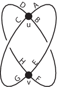
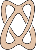
Figure 4: A fat graph Γ\Gamma and its surface ΣΓ\Sigma_{\Gamma}
Example 6.

As in figure 4, we consider the graph with two vertices uu and vv and whose half-edges are

H={A,B,C,D,E,F,G,H,}H=\{A,B,C,D,E,F,G,H,\}

The source map is

s⁡(A)=s⁡(B)=s⁡(C)=s⁡(D)=us⁡(E)=s⁡(F)=s⁡(G)=s⁡(H)=vs(A)=s(B)=s(C)=s(D)=u\qquad s(E)=s(F)=s(G)=s(H)=v

and the involution associates

i⁡(A)=Ei⁡(B)=Fi⁡(C)=Gi⁡(D)=H.i(A)=E\quad i(B)=F\quad i(C)=G\quad i(D)=H.

We put the fat structure

σ=(A​B​C​D)​(E​F​G​H)\sigma=(ABCD)(EFGH)

on GG which is given by the clockwise orientation on the plane. The boundary cycles of Γ\Gamma are then

ω=(A​F​C​H)​(B​G​D​E)\omega=(AFCH)(BGDE)

Hence the surface ΣΓ\Sigma_{\Gamma}, which is also pictured in ffigure 4, has two boundary components. Since ΣΓ\Sigma_{\Gamma} is homotopy equivalent to Γ\Gamma, its Euler characteristic is −2-2 and hence ΣΓ\Sigma_{\Gamma} is homeomorphic to a torus with two boundary components.

Igusa defined ℱ​𝑎𝑡{\mathcal{F}\hskip-2.0pt\mathit{at}} to be the category whose objects are fat graphs (Γ,ω)(\Gamma,\omega). We ask that every vertex of Γ\Gamma has valence at least three, ie there are at least three half-edges with source vv. The morphisms of ℱ​𝑎𝑡{\mathcal{F}\hskip-2.0pt\mathit{at}} are the morphism of fat graphs.

For any closed surface SS with marked points p1,…​pkp_{1},\ldots p_{k}, let the mapping class group of SS

𝑀𝑜𝑑⁡(S)=π0​𝐷𝑖𝑓𝑓+​(S,{p1,…​pk})\mathit{Mod}(S)=\pi_{0}\mathit{Diff}^{+}(S;\{p_{1},\ldots p_{k}\})

be the group of isotopy classes of diffeomorphisms of SS which fix the pip_{i}’s.

Theorem 2 (Harer, Strebel, Penner, Igusa).

The geometric realization of the category ℱ​𝑎𝑡{\mathcal{F}\hskip-2.0pt\mathit{at}} is

|ℱ​𝑎𝑡|≃∐[S]B​𝑀𝑜𝑑​(S)|{\mathcal{F}\hskip-2.0pt\mathit{at}}|\simeq\coprod_{[S]}B\mathit{Mod}(S)

a disjoint union of classifying space of the mapping class groups of marked surfaces with positive Euler characteristic. Here the disjoint union is over all diffeomorphism type of surfaces SS of genus gg with k≥1k\geq 1 marked points with negative Euler characteristic.

Remark 4.

We will let ℱ​𝑎𝑡g,s{\mathcal{F}\hskip-2.0pt\mathit{at}}_{g,s} be the subcategory which realizes to the connected component homotopy equivalent to B​𝑀𝑜𝑑​(S)B\mathit{Mod}(S) where SS is a connected surface of genus gg with ss marked points. The universal cover of |ℱ​𝑎𝑡g,s||{\mathcal{F}\hskip-2.0pt\mathit{at}}_{g,s}| is the geometric realization of the E​ℱ​𝑎𝑡g,sE{\mathcal{F}\hskip-2.0pt\mathit{at}}_{g,s} whose objects are pairs

(Γ,[f:|Γ|⟶S]).\left(\Gamma,[f:|\Gamma|\longrightarrow S]\right).

Here [f][f] is a isotopy classes of embeddings that avoid the marked points. We also asked that ff be a homotopy equivalence and that each marked point be circled by its corresponding boundary cycle. See [11, 10] for more details.

2.2 Open-closed fat graphs.

An open-closed cobordism SS is a surface with boundary. The boundary of SS is divided into an incoming ∂𝑖𝑛S\partial_{\mathit{in}}S, an outgoing ∂𝑜𝑢𝑡S\partial_{\mathit{out}}S and a free ∂𝑓𝑟𝑒𝑒S\partial_{\mathit{free}}S parts. Hence, SS is a cobordism between the 1-manifolds with boundary ∂𝑖𝑛S\partial_{\mathit{in}}S and ∂𝑜𝑢𝑡S\partial_{\mathit{out}}S. The remainder ∂𝑓𝑟𝑒𝑒S\partial_{\mathit{free}}S is a cobordism between the boundary of ∂𝑖𝑛S\partial_{\mathit{in}}S and ∂𝑜𝑢𝑡S\partial_{\mathit{out}}S. The mapping class group of such an SS is the group

𝑀𝑜𝑑⁡(S)=π0​𝐷𝑖𝑓𝑓+​(S,∂𝑖𝑛S∐∂𝑜𝑢𝑡S)\mathit{Mod}(S)=\pi_{0}\mathit{Diff}^{+}(S;\partial_{\mathit{in}}S\amalg\partial_{\mathit{out}}S)

of isotopy classes of diffeomorphisms of SS which fixes the incoming and the outgoing boundary components pointwise.

In this section we will decorate the fat graphs of ℱ​𝑎𝑡{\mathcal{F}\hskip-2.0pt\mathit{at}} to construct a category ℱ​𝑎𝑡𝑜𝑐{\mathcal{F}\hskip-2.0pt\mathit{at}}^{\mathit{oc}} of open-closed fat graphs. The connected components of the geometric realization of ℱ​𝑎𝑡𝑜𝑐{\mathcal{F}\hskip-2.0pt\mathit{at}}^{{\mathit{oc}}} are homotopy equivalent to the classifying spaces of the different open-closed mapping class groups 𝑀𝑜𝑑⁡(S)\mathit{Mod}(S).

Let GG be a graph. A vertex vv of GG is called a leaf if it has valence one, ie if there is a single edge attach to it. We let Vl⊂VV_{l}\subset V be the set of leaf of GG. An open-closed fat graph is a quadruple

(Γ,ℐ​n,𝒪​𝑢𝑡,𝒞​𝑙𝑜𝑠𝑒𝑑)\left(\Gamma,\mathcal{I}\hskip-2.0pt\mathit{n},\mathcal{O}\hskip-2.0pt\mathit{ut},\mathcal{C}\hskip-2.0pt\mathit{losed}\right)

where Γ=(G,ω)\Gamma=(G,\omega) is a fat graph and

ℐ​n,𝒪​𝑢𝑡,𝒞​𝑙𝑜𝑠𝑒𝑑⊂Vl\mathcal{I}\hskip-2.0pt\mathit{n},\mathcal{O}\hskip-2.0pt\mathit{ut},\mathcal{C}\hskip-2.0pt\mathit{losed}\subset V_{l}

are all subsets of the set of leaves in GG. We require that ℐ​n\mathcal{I}\hskip-2.0pt\mathit{n} and 𝒪​𝑢𝑡\mathcal{O}\hskip-2.0pt\mathit{ut} be disjoint and ordered. We will call the elements of ℐ​n\mathcal{I}\hskip-2.0pt\mathit{n} incoming leaves and the elements of 𝒪​𝑢𝑡\mathcal{O}\hskip-2.0pt\mathit{ut}, outgoing leaves. We will call a leaf special if it is either incoming or outgoing. We also require that the closed leaves all be special

𝒞​𝑙𝑜𝑠𝑒𝑑⊂ℐ​n∪𝒪​𝑢𝑡=:𝒮​𝑝𝑒𝑐𝑖𝑎𝑙\mathcal{C}\hskip-2.0pt\mathit{losed}\subset\mathcal{I}\hskip-2.0pt\mathit{n}\cup\mathcal{O}\hskip-2.0pt\mathit{ut}=:\mathcal{S}\hskip-2.0pt\mathit{pecial}

and that each leaf vv in 𝒞​𝑙𝑜𝑠𝑒𝑑\mathcal{C}\hskip-2.0pt\mathit{losed} be the only special leaf in its boundary cycle. The special leaves that are not closed are said to be open

𝒪​𝑝𝑒𝑛=𝒮​𝑝𝑒𝑐𝑖𝑎𝑙∖𝒞​𝑙𝑜𝑠𝑒𝑑.\mathcal{O}\hskip-2.0pt\mathit{pen}=\mathcal{S}\hskip-2.0pt\mathit{pecial}\setminus\mathcal{C}\hskip-2.0pt\mathit{losed}.

This extra data on Γ\Gamma gives S=ΣΓS=\Sigma_{\Gamma} the structure of an open-closed cobordism as follows. We first divide the boundary into the three parts ∂𝑖𝑛S\partial_{\mathit{in}}S, ∂𝑜𝑢𝑡S\partial_{\mathit{out}}S and ∂𝑓𝑟𝑒𝑒S\partial_{\mathit{free}}S. The incoming boundary is made up of the entire boundary associated to a closed incoming leaf and a small part

{[(0,h),(t,h)]∈∂ht≤1/2s(h)=v}∪{[(0,h),(t,h)]∈∂ht≥1/2s(i(h))=v}\Big\{[(0,h),(t,h)]\in\partial_{h}\quad t\leq 1/2\quad s(h)=v\Big\}\cup\Big\{[(0,h),(t,h)]\in\partial_{h}\quad t\geq 1/2\quad s(i(h))=v\Big\}

of the boundary around an open incoming leaf.

Refer to caption  Refer to caption

Figure 5: An open-closed fat graph and its associated open-closed cobordism.
Example 7.

The fat graph of figure 5 has five leaves

Vl={u,v,x,y,z}V_{l}=\{u,v,x,y,z\}

and four boundary cycles ωu\omega_{u}, ωv\omega_{v}, ωx,z\omega_{x,z}, ωy\omega_{y}. We let

ℐ​n={v,z}𝒪​𝑢𝑡={x,y}𝒞​𝑙𝑜𝑠𝑒𝑑={v}𝒪​𝑝𝑒𝑛={x,y,z}.\mathcal{I}\hskip-2.0pt\mathit{n}=\{v,z\}\qquad\mathcal{O}\hskip-2.0pt\mathit{ut}=\{x,y\}\qquad\mathcal{C}\hskip-2.0pt\mathit{losed}=\{v\}\qquad\mathcal{O}\hskip-2.0pt\mathit{pen}=\{x,y,z\}.

The open-closed cobordism ΣΓ\Sigma_{\Gamma} is also illustrated in figure 5. The incoming and outgoing boundary are thickened while the free boundary is thin. In particular ΣΓ\Sigma_{\Gamma} is a cobordism between

I∐S1⟶I∐I.I\amalg S^{1}\longrightarrow I\amalg I.

A morphism of open-closed fat graph

φ:(Γ0,ℐ​n0,𝒪​𝑢𝑡0,𝒞​𝑙𝑜𝑠𝑒𝑑0)⟶(Γ1,ℐ​n1,𝒪​𝑢𝑡1,𝒞​𝑙𝑜𝑠𝑒𝑑1)\varphi:\left(\Gamma_{0},\mathcal{I}\hskip-2.0pt\mathit{n}_{0},\mathcal{O}\hskip-2.0pt\mathit{ut}_{0},\mathcal{C}\hskip-2.0pt\mathit{losed}_{0}\right)\longrightarrow\left(\Gamma_{1},\mathcal{I}\hskip-2.0pt\mathit{n}_{1},\mathcal{O}\hskip-2.0pt\mathit{ut}_{1},\mathcal{C}\hskip-2.0pt\mathit{losed}_{1}\right)

is a morphism of fat graphs φ:Γ0⟶Γ1\varphi:\Gamma_{0}\longrightarrow\Gamma_{1} which induces order-preserving isomorphism

φ𝑖𝑛:ℐ​n0​⟶≅​ℐ​n1φ𝑜𝑢𝑡:𝒪​𝑢𝑡0​⟶≅​𝒪​𝑢𝑡1φ𝑐𝑙𝑜𝑠𝑒𝑑:𝒞​𝑙𝑜𝑠𝑒𝑑0​⟶≅​𝒞​𝑙𝑜𝑠𝑒𝑑1.\varphi_{\mathit{in}}:\mathcal{I}\hskip-2.0pt\mathit{n}_{0}\overset{\cong}{\longrightarrow}\mathcal{I}\hskip-2.0pt\mathit{n}_{1}\qquad\varphi_{\mathit{out}}:\mathcal{O}\hskip-2.0pt\mathit{ut}_{0}\overset{\cong}{\longrightarrow}\mathcal{O}\hskip-2.0pt\mathit{ut}_{1}\qquad\varphi_{\mathit{closed}}:\mathcal{C}\hskip-2.0pt\mathit{losed}_{0}\overset{\cong}{\longrightarrow}\mathcal{C}\hskip-2.0pt\mathit{losed}_{1}.

Let ℱ​𝑎𝑡𝑜𝑐{\mathcal{F}\hskip-2.0pt\mathit{at}}^{{\mathit{oc}}} be the category of open-closed fat graphs with these morphisms.

Theorem 3.

The geometric realization of the category ℱ​𝑎𝑡𝑜𝑐{\mathcal{F}\hskip-2.0pt\mathit{at}}^{{\mathit{oc}}} of open-closed

|ℱ​𝑎𝑡𝑜𝑐|≃∐[S]B​𝑀𝑜𝑑𝑜𝑐​(S)|{\mathcal{F}\hskip-2.0pt\mathit{at}}^{{\mathit{oc}}}|\simeq\coprod_{[S]}B\mathit{Mod}^{{\mathit{oc}}}(S)

a disjoint union of classifying spaces of open-closed mapping class group. More precisely, the disjoint union is over all diffeomorphism of open-closed cobordism [S][S] with ordered incoming and outgoing boundary components.

Proof.

First we claim that allowing for univalent and bivalent vertices in Igusa’s category does not change the homotopy type of the geometric realization. Consider the categories ℱ​𝑎𝑡1,2{\mathcal{F}\hskip-2.0pt\mathit{at}}^{1,2} and ℱ​𝑎𝑡2{\mathcal{F}\hskip-2.0pt\mathit{at}}^{2} whose objects are respectively any fat graph and fat graphs with no univalent vertices.

Lets first show that removing univalent vertices does not change the homotopy type. There are two functors

ℱ​𝑎𝑡1,2​⟶ξ1​ℱ​𝑎𝑡2​⟶ξ2​ℱ​𝑎𝑡1,2.{\mathcal{F}\hskip-2.0pt\mathit{at}}^{1,2}\overset{\xi_{1}}{\longrightarrow}{\mathcal{F}\hskip-2.0pt\mathit{at}}^{2}\overset{\xi_{2}}{\longrightarrow}{\mathcal{F}\hskip-2.0pt\mathit{at}}^{1,2}.

The functor ξ2\xi_{2} is the natural inclusion. The functor ξ1\xi_{1} removes all univalent vertices and the unique edge leading to it. And repeats this process until there are no univalent vertices. The composition ξ1⋅ξ2\xi_{1}\cdot\xi_{2} is the identity. There is a natural transformation θ\theta between the composition the identity on ℱ​𝑎𝑡1,2{\mathcal{F}\hskip-2.0pt\mathit{at}}^{1,2} and ξ2⋅ξ1\xi_{2}\cdot\xi_{1} by collapsing all the edges that ξ2⋅ξ1\xi_{2}\cdot\xi_{1} has removed.

Lets now shoe that we can remove bivalent vertices as well.There are also two functors

ℱ​𝑎𝑡2​⟶ξ3​ℱ​𝑎𝑡​⟶ξ4​ℱ​𝑎𝑡2.{\mathcal{F}\hskip-2.0pt\mathit{at}}^{2}\overset{\xi_{3}}{\longrightarrow}{\mathcal{F}\hskip-2.0pt\mathit{at}}\overset{\xi_{4}}{\longrightarrow}{\mathcal{F}\hskip-2.0pt\mathit{at}}^{2}.

The functor ξ4\xi_{4} is the natural inclusion. The functor ξ3\xi_{3} takes a fat graph Γ=(G,σ=(σv))\Gamma=(G,\sigma=(\sigma_{v})) to the fat graph Γ𝑢𝑛𝑖𝑡𝑒𝑑\Gamma^{{\mathit{united}}} obtained from removing all bivalent vertices vv and joining the two edges attaching at vv into a single edge. Again the composition ξ3⋅ξ4\xi_{3}\cdot\xi_{4} is the identity. It therefore suffices to show that ζ=ξ3\zeta=\xi_{3} is a homotopy equivalence.

To show this, we will prove that the geometric realization of the over category ζ/Γ\zeta/\Gamma is contractible for each Γ\Gamma in ℱ​𝑎𝑡{\mathcal{F}\hskip-2.0pt\mathit{at}}. The objects of ζ/Γ\zeta/\Gamma are pairs (Γ~,φ)({\widetilde{\Gamma}},\varphi) where Γ~{\widetilde{\Gamma}} is a fat graph with no leaves (but with possibly bivalent vertices) and where

φ:ζ⁡(Γ~)⟶Γ\varphi:\zeta({\widetilde{\Gamma}})\longrightarrow\Gamma

is a morphism of fat graph between two fat graphs with no univalent or bivalent vertices. The morphism

φ~:(Γ~0,φ0)⟶(Γ~1,φ1){\widetilde{\varphi}}:({\widetilde{\Gamma}}_{0},\varphi_{0})\longrightarrow({\widetilde{\Gamma}}_{1},\varphi_{1})

of ζ/Γ\zeta/\Gamma are morphism

φ~:Γ~0⟶Γ~1{\widetilde{\varphi}}:{\widetilde{\Gamma}}_{0}\longrightarrow{\widetilde{\Gamma}}_{1}

of fat graphs that make the following diagram commute.

ζ⁡(Γ~0)\textstyle{\zeta({\widetilde{\Gamma}}_{0})\ignorespaces\ignorespaces\ignorespaces\ignorespaces\ignorespaces\ignorespaces\ignorespaces\ignorespaces}ζ⁡(φ~)\scriptstyle{\zeta({\widetilde{\varphi}})}φ0\scriptstyle{\varphi_{0}}Γ\textstyle{\Gamma}ζ⁡(Γ~1).\textstyle{\zeta({\widetilde{\Gamma}}_{1})\ignorespaces\ignorespaces\ignorespaces\ignorespaces.}φ1\scriptstyle{\varphi_{1}}

Let 𝒞Γ\mathcal{C}_{\Gamma} be the full subcategory of ζ/Γ\zeta/\Gamma whose objects are the pairs (Γ~,φ)({\widetilde{\Gamma}},\varphi) where φ\varphi is an isomorphism. We claim that 𝒞Γ\mathcal{C}_{\Gamma} is a deformation retract of ζ/Γ\zeta/\Gamma. Note that the objects of the category 𝒞Γ\mathcal{C}_{\Gamma} give a subdivision of Γ\Gamma by adding bivalent vertices. Let FF be the functor

F:ζ/Γ⟶𝒞ΓF:\zeta/\Gamma\longrightarrow\mathcal{C}_{\Gamma}

which takes an object (Γ~,φ:ζ(Γ~)⟶Γ)({\widetilde{\Gamma}},\varphi:\zeta({\widetilde{\Gamma}})\longrightarrow\Gamma) to the fat graph above Γ\Gamma obtained by collapsing every subdivision of every edge collapsed by φ\varphi. This gives both the functor and the natural transformation back to the identity.

It now suffices to show that for any Γ\Gamma, the two functors

𝒞Γ\textstyle{\mathcal{C}_{\Gamma}\ignorespaces\ignorespaces\ignorespaces\ignorespaces\ignorespaces\ignorespaces\ignorespaces\ignorespaces}I​d\scriptstyle{Id}c​s​t\scriptstyle{cst}𝒞Γ\textstyle{\mathcal{C}_{\Gamma}}

where c​s​tcst is the constant functor which sends anything to (Γ,I​d)(\Gamma,Id) induces homotopy equivalent maps on the realization. To do so, we first pick arbitrary orientations of every edge of Γ\Gamma. Following an argument of Igusa [11, Chapter 8], we then construct an intermediary functor

F:𝒞Γ⟶𝒞ΓF:\mathcal{C}_{\Gamma}\longrightarrow\mathcal{C}_{\Gamma}

which sends (Γ~,φ)({\widetilde{\Gamma}},\varphi) to the fat graph obtained by adding a new edge and a new bivalent vertex at the beginning of every edge of Γ\Gamma. (Here we are using the arbitrary choice of an orientation.) We have natural transformation

I​d\textstyle{Id}F\textstyle{\ignorespaces\ignorespaces\ignorespaces\ignorespaces F\ignorespaces\ignorespaces\ignorespaces\ignorespaces}ν1\scriptstyle{\nu_{1}}ν2\scriptstyle{\nu_{2}}c​s​t.\textstyle{cst.}

Here ν1\nu_{1} collapses the newly added edges while ν2\nu_{2} collapses every other edge. This shows that adding bivalent and univalent vertices does not change the homotopy type of the geometric realization.

The rest of the proof is a slight variant from [10]. Fix an open-closed cobordism SS. Denote by S~\tilde{S} the marked surface obtained from SS by collapsing each boundary component to a marked point. The maked points are divided into ℳ​𝑎𝑟𝑘𝑒𝑑𝑠𝑝𝑒𝑐𝑖𝑎𝑙\mathcal{M}\hskip-1.0pt{\mathit{arked}}_{{\mathit{special}}} and ℳ​𝑎𝑟𝑘𝑒𝑑𝑓𝑟𝑒𝑒\mathcal{M}\hskip-1.0pt{\mathit{arked}}_{\mathit{free}} depending on whether their corresponding boundary contains an incoming or outgoing boundary or whether it does not. (Note that the entire boundary must be free for a marked point to be considered free.)

Recall that 𝑀𝑜𝑑⁡(S~)\mathit{Mod}(\tilde{S}) is the mapping class group of diffeomorphisms which preserve each marked point. Consider the mapping class groups 𝑀𝑜𝑑𝑓𝑟𝑒𝑒​(S~)\mathit{Mod}^{\mathit{free}}(\tilde{S}) associated to the diffeomorphisms which preserves 𝑓𝑟𝑒𝑒\mathit{free} as a set and fixes every special marked point. We have a short exact sequence of groups

0⟶𝑀𝑜𝑑⁡(S~)⟶𝑀𝑜𝑑𝑓𝑟𝑒𝑒​(S~)⟶Σ⁡(𝑓𝑟𝑒𝑒)⟶00\longrightarrow\mathit{Mod}(\tilde{S})\longrightarrow\mathit{Mod}^{\mathit{free}}(\tilde{S})\longrightarrow\Sigma(\mathit{free})\longrightarrow 0

where Σ⁡(A)\Sigma(A) is the group of permutations on the set AA. On the classifying spaces, we get a homotopy fibration

Σ⁡(𝑓𝑟𝑒𝑒)\textstyle{\Sigma(\mathit{free})\ignorespaces\ignorespaces\ignorespaces\ignorespaces}B​𝑀𝑜𝑑​(S~)\textstyle{B\mathit{Mod}(\tilde{S})\ignorespaces\ignorespaces\ignorespaces\ignorespaces}B​𝑀𝑜𝑑𝑓𝑟𝑒𝑒​(S~)\textstyle{B\mathit{Mod}^{\mathit{free}}(\tilde{S})}

Fix an ordering on the marked points of S~\tilde{S} so that the special ones p1,…​pkp_{1},\ldots p_{k} come first. Consider the category ℱ​𝑎𝑡S𝑓𝑟𝑒𝑒{\mathcal{F}\hskip-2.0pt\mathit{at}}^{\mathit{free}}_{S} whose objects are fat graphs with a splitting of the boundary cycles into special ones and free ones. We give the special boundary cycles an ordering which is preserved by the morphisms of ℱ​𝑎𝑡S𝑓𝑟𝑒𝑒{\mathcal{F}\hskip-2.0pt\mathit{at}}^{\mathit{free}}_{S}. We only take fat graphs so that the surface ΣΓ\Sigma_{\Gamma} is homeomorphic to S as surfaces and that the number of special boundary cycles in Γ\Gamma is the number of special mark points in S~\tilde{S}. Note that the morphism of ℱ​𝑎𝑡S𝑓𝑟𝑒𝑒{\mathcal{F}\hskip-2.0pt\mathit{at}}^{\mathit{free}}_{S} are allowed to interchange the boundary cycles of 𝑓𝑟𝑒𝑒\mathit{free}. Hence there is a functor

ξ:ℱ​𝑎𝑡S⟶ℱ​𝑎𝑡S𝑓𝑟𝑒𝑒\xi\ :\ {\mathcal{F}\hskip-2.0pt\mathit{at}}_{S}\longrightarrow{\mathcal{F}\hskip-2.0pt\mathit{at}}^{\mathit{free}}_{S}

which sends the object (Γ,ω1,ω2​…​ωn)(\Gamma,\omega_{1},\omega_{2}\ldots\omega_{n}) to the same fat graph Γ\Gamma with special cycles ω1​…​ωk\omega_{1}\,\ldots\omega_{k} ordered as before. The fiber above each Γ\Gamma is simply a choice of ordering on the remaining boundary cycles and hence is (not naturally) isomorphic to Σ⁡(𝑓𝑟𝑒𝑒)\Sigma(\mathit{free}). Any morphism of ℱ​𝑎𝑡S𝑓𝑟𝑒𝑒{\mathcal{F}\hskip-2.0pt\mathit{at}}^{\mathit{free}}_{S} lifts to a bijection between the two corresponding fibers. Hence we get a covering space

Σ⁡(𝑓𝑟𝑒𝑒)\textstyle{\Sigma(\mathit{free})\ignorespaces\ignorespaces\ignorespaces\ignorespaces}|ℱ​𝑎𝑡S|\textstyle{|{\mathcal{F}\hskip-2.0pt\mathit{at}}_{S}|\ignorespaces\ignorespaces\ignorespaces\ignorespaces}|ℱ​𝑎𝑡S𝑓𝑟𝑒𝑒|.\textstyle{|{\mathcal{F}\hskip-2.0pt\mathit{at}}^{\mathit{free}}_{S}|.}

Since the two fibrations lift to the universal cover in exactly the same way we get that

|ℱ​𝑎𝑡S𝑓𝑟𝑒𝑒|≃B​𝑀𝑜𝑑𝑓𝑟𝑒𝑒​(S~).|{\mathcal{F}\hskip-2.0pt\mathit{at}}^{\mathit{free}}_{S}|\simeq B\mathit{Mod}^{\mathit{free}}(\tilde{S}).

Now every diffeomorphism of SS induces one on S~\tilde{S} which gives a group homomorphism

𝑀𝑜𝑑𝑜𝑐​(S)⟶𝑀𝑜𝑑𝑓𝑟𝑒𝑒​(S~).\mathit{Mod}^{{\mathit{oc}}}(S)\longrightarrow\mathit{Mod}^{\mathit{free}}(\tilde{S}).

Since all these mapping class groups are generated by Dehn twists, this homomorphism is surjective. Its kernel is generated by Dehn twists around the boundary components. This gives a central extension

0⟶ℤπ0​(∂𝑠𝑝𝑒𝑐𝑖𝑎𝑙S)⟶𝑀𝑜𝑑𝑜𝑐​(S)⟶𝑀𝑜𝑑⁡(S~)⟶0.0\longrightarrow\mathbb{Z}^{\pi_{0}(\partial_{\mathit{special}}S)}\longrightarrow\mathit{Mod}^{{\mathit{oc}}}(S)\longrightarrow\mathit{Mod}(\tilde{S})\longrightarrow 0.

On the classifying spaces, we get a fibration

(S1)π0​(∂𝑠𝑝𝑒𝑐𝑖𝑎𝑙S)≅B​ℤπ0​(∂𝑠𝑝𝑒𝑐𝑖𝑎𝑙S)\textstyle{(S^{1})^{\pi_{0}(\partial_{\mathit{special}}S)}\cong B\mathbb{Z}^{\pi_{0}(\partial_{\mathit{special}}S)}\ignorespaces\ignorespaces\ignorespaces\ignorespaces}B​𝑀𝑜𝑑𝑜𝑐​(S)\textstyle{B\mathit{Mod}^{\mathit{oc}}(S)\ignorespaces\ignorespaces\ignorespaces\ignorespaces}B​𝑀𝑜𝑑​(S~)\textstyle{B\mathit{Mod}(\tilde{S})}

We shall define a functor

Ψ:ℱ​𝑎𝑡𝑜𝑐⟶ℱ​𝑎𝑡\Psi:{\mathcal{F}\hskip-2.0pt\mathit{at}}^{{\mathit{oc}}}\longrightarrow{\mathcal{F}\hskip-2.0pt\mathit{at}}

which will realize this fibration on the categories.

First fix an open-closed cobordism SS. Pick an ordering on the components π0​∂𝑖𝑛S\pi_{0}\partial_{\mathit{in}}S of the incoming boundary, the components π0​∂𝑖𝑛S\pi_{0}\partial_{\mathit{in}}S and an ordering on the special boundary components π0​∂𝑠𝑝𝑒𝑐𝑖𝑎𝑙S\pi_{0}\partial_{\mathit{special}}S of SS. Let ℱ​𝑎𝑡S𝑜𝑐{\mathcal{F}\hskip-2.0pt\mathit{at}}^{{\mathit{oc}}}_{S} be the category of fat graphs Γ𝑜𝑐=(Γ,ℐ​n,𝒪​𝑢𝑡,𝒞​𝑙𝑜𝑠𝑒𝑑)\Gamma^{{\mathit{oc}}}=(\Gamma,\mathcal{I}\hskip-2.0pt\mathit{n},\mathcal{O}\hskip-2.0pt\mathit{ut},\mathcal{C}\hskip-2.0pt\mathit{losed}) whose associated open-closed cobordism §Γ𝑜𝑐\lx@sectionsign_{\Gamma^{\mathit{oc}}} is homeomorphic to SS as open-closed cobordism.

Take any open-closed fat graphs (Γ,ℐ​n,𝒪​𝑢𝑡,𝒞​𝑙𝑜𝑠𝑒𝑑)(\Gamma,\mathcal{I}\hskip-2.0pt\mathit{n},\mathcal{O}\hskip-2.0pt\mathit{ut},\mathcal{C}\hskip-2.0pt\mathit{losed}) in ℱ​𝑎𝑡S𝑜𝑐{\mathcal{F}\hskip-2.0pt\mathit{at}}^{{\mathit{oc}}}_{S}. Since ℐ​n\mathcal{I}\hskip-2.0pt\mathit{n} is ordered, there is a natural bijection

ℐ​n≅π0​∂𝑖𝑛S\mathcal{I}\hskip-2.0pt\mathit{n}\cong\pi_{0}\partial_{\mathit{in}}S

and similarly, we get

𝒪​𝑢𝑡≅π0​∂𝑜𝑢𝑡S.\mathcal{O}\hskip-2.0pt\mathit{ut}\cong\pi_{0}\partial_{\mathit{out}}S.

In particular this fixes a bijection between the special boundary components of SS and the ones of ΣΓ\Sigma_{\Gamma}. Using the ordering on π0​∂𝑠𝑝𝑒𝑐𝑖𝑎𝑙S\pi_{0}\partial_{\mathit{special}}S, we get an ordering of the special boundary cycles of Γ\Gamma.

Define Ψ⁡(Γ𝑜𝑐)\Psi(\Gamma^{{\mathit{oc}}}) to be the fat graph Γ~{\widetilde{\Gamma}} obtained from Γ\Gamma by removing all the special leaves in ℐ​n∪𝒪​𝑢𝑡\mathcal{I}\hskip-2.0pt\mathit{n}\cup\mathcal{O}\hskip-2.0pt\mathit{ut} and the unique edge leading to them. If that special edge was attached to a trivalent vertex, we remove this (now bivalent) vertex. The special boundary cycles of Γ~{\widetilde{\Gamma}} are the ones corresponding to special boundary cycles in Γ\Gamma and these are ordered.

Fix a fat graph Γ~{\widetilde{\Gamma}} in ℱ​𝑎𝑡S{\mathcal{F}\hskip-2.0pt\mathit{at}}_{S}. Lets study the category Ψ/Γ~\Psi/{\widetilde{\Gamma}}. An object of Ψ/Γ~\Psi/{\widetilde{\Gamma}} is a pair

(Γ𝑜𝑐,φ:Ψ(Γ𝑜𝑐)⟶Γ~).\left(\Gamma^{{\mathit{oc}}},\varphi:\Psi(\Gamma^{\mathit{oc}})\longrightarrow{\widetilde{\Gamma}}\right).

As before, we define a functor

J:Ψ/Γ~⟶Ψ−1​(Γ~)J:\Psi/{\widetilde{\Gamma}}\longrightarrow\Psi^{-1}({\widetilde{\Gamma}})

by sending (Γ𝑜𝑐,φ)(\Gamma^{{\mathit{oc}}},\varphi) to the open-closed fat graph obtained by collapsing in Γ𝑜𝑐\Gamma^{{\mathit{oc}}} the edges collapsed in Ψ⁡(Γ𝑜𝑐)\Psi(\Gamma^{{\mathit{oc}}}) by φ\varphi. It is easy to show that JJ is adjoint to the inclusion

I:Ψ−1​(Γ~)⟶Ψ/Γ~I:\Psi^{-1}({\widetilde{\Gamma}})\longrightarrow\Psi/{\widetilde{\Gamma}}

and in particular, to use Quillen’s theorem B, it suffices to show that any morphism

ψ:Γ~1⟶Γ~2\psi:{\widetilde{\Gamma}}_{1}\longrightarrow{\widetilde{\Gamma}}_{2}

of ℱ​𝑎𝑡S{\mathcal{F}\hskip-2.0pt\mathit{at}}_{S} induces an homotopy equivalence

ψ∗:|Ψ−1​(Γ~1)|⟶|Ψ−1​(Γ~2)|.\psi^{*}:|\Psi^{-1}({\widetilde{\Gamma}}_{1})|\longrightarrow|\Psi^{-1}({\widetilde{\Gamma}}_{2})|.

To do this we will show that for any Γ~{\widetilde{\Gamma}} in ℱ​𝑎𝑡S{\mathcal{F}\hskip-2.0pt\mathit{at}}_{S}

|Ψ−1​(Γ~)|≃(S1)∂𝑠𝑝𝑒𝑐𝑖𝑎𝑙S.|\Psi^{-1}({\widetilde{\Gamma}})|\simeq\left(S^{1}\right)^{\partial_{\mathit{special}}S}.

Since the special boundary cycle of Γ~{\widetilde{\Gamma}} are ordered, they correspond to special boundary component of SS. To get an object in Ψ−1​(Γ~)\Psi^{-1}({\widetilde{\Gamma}}), we need to attach leaves on each of these boundary cycles one for each incoming or outgoing parts. For example, if the i𝑡ℎi^{\mathit{th}} boundary component of SS has four special intervals on it which alternate between incoming and outgoing as someone walks along the boundary. Say that these intervals are number 2nd, 2nd, 3rd, 3rd (recall that incoming and outgoing are ordered separately). Then we need to pick along the i𝑡ℎi^{\mathit{th}} boundary of Γ~{\widetilde{\Gamma}} four attaching points for the leaves

l2𝑖𝑛l2𝑜𝑢𝑡l3𝑖𝑛l3𝑜𝑢𝑡.l_{2}^{\mathit{in}}\quad l_{2}^{\mathit{out}}\quad l_{3}^{\mathit{in}}\quad l_{3}^{\mathit{out}}.

This corresponds to choosing fourf cyclically ordered points on the circle of ωi\omega_{i}. This choice is therefore, up to homotopy, a circle. ∎

2.3 Admissible fat graphs

Following the definition of the Sullivan chord diagrams in [3], we now restrict the shape of the graph underlying an open-closed fat graph. These admissible fat graphs will be used to define the higher genus string operations in the following sections. Note that this model is quite similar to the model used in [7].

Definition 1.

An open-closed fat graph

Γ𝑜𝑐=(Γ,ℐ​n,𝒪​𝑢𝑡,𝒞​𝑙𝑜𝑠𝑒𝑑)\Gamma^{{\mathit{oc}}}=(\Gamma,\mathcal{I}\hskip-2.0pt\mathit{n},\mathcal{O}\hskip-2.0pt\mathit{ut},\mathcal{C}\hskip-2.0pt\mathit{losed})

is admissible if its incoming boundary cycles are embedded in Γ\Gamma.

More precisely each incoming leaf vv in ℐ​n∩𝒞​𝑙𝑜𝑠𝑒𝑑\mathcal{I}\hskip-2.0pt\mathit{n}\ \cap\ \mathcal{C}\hskip-2.0pt\mathit{losed}, which represent a closed incoming boundary component of ΣΓ\Sigma_{\Gamma}, correspond to some boundary cycle of Γ\Gamma and hence to a map

fv:S1⟶|Γ|.f_{v}:S^{1}\longrightarrow|\Gamma|.

We get a map

∐v∈ℐ​n∖𝒞​𝑙𝑜𝑠𝑒𝑑​{v}∐∐v∈ℐ​n∩𝒞​𝑙𝑜𝑠𝑒𝑑​S1\textstyle{\underset{v\in\mathcal{I}\hskip-2.0pt\mathit{n}\setminus\mathcal{C}\hskip-2.0pt\mathit{losed}}{\coprod}\{v\}\amalg\underset{v\in\mathcal{I}\hskip-2.0pt\mathit{n}\cap\mathcal{C}\hskip-2.0pt\mathit{losed}}{\coprod}S^{1}\ignorespaces\ignorespaces\ignorespaces\ignorespaces}∐I​d∐∐fv\scriptstyle{\coprod Id\amalg\coprod f_{v}}|Γ|.\textstyle{|\Gamma|.}

The open-closed fat graph Γ𝑜𝑐\Gamma^{{\mathit{oc}}} is admissible if and only if this map is an inclusion.

Refer to caption

Figure 6: A fat graph
Example 8.

Let Γ\Gamma be the fat graph of figure 6. An open-closed fat graph Γ𝑜𝑐=(Γ,ℐ​n,𝒪​𝑢𝑡,𝒞​𝑙𝑜𝑠𝑒𝑑)\Gamma^{\mathit{oc}}=(\Gamma,\mathcal{I}\hskip-2.0pt\mathit{n},\mathcal{O}\hskip-2.0pt\mathit{ut},\mathcal{C}\hskip-2.0pt\mathit{losed}) is admissible if and only if

ℐ​n∩𝒞​𝑙𝑜𝑠𝑒𝑑⊂{x,y}.\mathcal{I}\hskip-2.0pt\mathit{n}\cap\mathcal{C}\hskip-2.0pt\mathit{losed}\subset\{x,y\}.

Let ℱ​𝑎𝑡a{\mathcal{F}\hskip-2.0pt\mathit{at}}^{a} be the full subcategory of ℱ​𝑎𝑡𝑜𝑐{\mathcal{F}\hskip-2.0pt\mathit{at}}^{{\mathit{oc}}} whose objects are all admissible fat graphs. For any open-closed cobordism SS, we denote by

ℱ​𝑎𝑡Sa=ℱ​𝑎𝑡a∩ℱ​𝑎𝑡S𝑜𝑐{\mathcal{F}\hskip-2.0pt\mathit{at}}^{a}_{S}={\mathcal{F}\hskip-2.0pt\mathit{at}}^{a}\cap{\mathcal{F}\hskip-2.0pt\mathit{at}}^{{\mathit{oc}}}_{S}

the subcategory of ℱ​𝑎𝑡a{\mathcal{F}\hskip-2.0pt\mathit{at}}^{a} whose open-closed fat graph Γ𝑜𝑐\Gamma^{{\mathit{oc}}} have a surface ΣΓ𝑜𝑐\Sigma_{\Gamma^{{\mathit{oc}}}} homeomorphic to SS as an open-closed cobordism.

Theorem 4.

For any open-closed cobordism SS whose boundary is not completely incoming, the inclusion

ℱ​𝑎𝑡Sa⟶ℱ​𝑎𝑡S𝑜𝑐{\mathcal{F}\hskip-2.0pt\mathit{at}}^{a}_{S}\longrightarrow{\mathcal{F}\hskip-2.0pt\mathit{at}}^{{\mathit{oc}}}_{S}

is a homotopy equivalence.

Proof.

It suffices to show this result for connected surfaces. So let SS be a connected open-closed cobordism. Say the surfaces SS has pp closed incoming boundary components, qq other boundary components and genus gg. By the assumption, qq is at least one.

We will first prove a similar statement for the mapping class group of the surface S′S^{\prime} obtained from SS by collapsing each boundary component to a marked point.

As before let ℱ​𝑎𝑡q,g2{\mathcal{F}\hskip-2.0pt\mathit{at}}^{2}_{q,g} be the category of fat graphs Γ\Gamma with qq ordered boundary cycles and whose surface ΣΓ\Sigma_{\Gamma} has genus gg. As in the previous section, we allow bivalent and univalent vertices. We already know that

|ℱ​𝑎𝑡q,g2|≃B​𝑀𝑜𝑑​(Sq,g)|{\mathcal{F}\hskip-2.0pt\mathit{at}}^{2}_{q,g}|\simeq B\mathit{Mod}(S_{q,g})

where Sq,gS_{q,g} is a connected surface with qq marked points and with genus gg. Lets also consider the category ℱq,gp\mathcal{F}^{p}_{q,g} of pairs (Γ,{v1,…​vp})(\Gamma,\{v_{1},\ldots v_{p}\}) where Γ\Gamma is a fat graph in ℱ​𝑎𝑡q,g{\mathcal{F}\hskip-2.0pt\mathit{at}}_{q,g} and where

{v1,…,vp}⊂V\{v_{1},\ldots,v_{p}\}\subset V

is an ordered set of pp distinct vertices in Γ\Gamma. The morphisms of ℱq,gp\mathcal{F}^{p}_{q,g} are morphisms of fat graphs which sends each marked vertex to the corresponding marked vertex.

A diffeomorphisms of Sp+q,gS_{p+q,g} which fixes p+qp+q marked points does fix qq points. We therefore get a short exact sequence

𝐷𝑖𝑓𝑓+​(Sp+q,g)⟶𝐷𝑖𝑓𝑓+​(Sq,g)​⟶e​vp​Cp​(Sq,g)\mathit{Diff}^{+}(S_{p+q,g})\longrightarrow\mathit{Diff}^{+}(S_{q,g})\overset{ev_{p}}{\longrightarrow}C_{p}(S_{q,g})

where Cp​(Sq,g)C_{p}(S_{q,g}) is the space of pp distinct and ordered points on SS. Since q>0q>0, we have that the connected components of 𝐷𝑖𝑓𝑓+​(Sp+q,g)\mathit{Diff}^{+}(S_{p+q,g}) are trivial and hence

𝐷𝑖𝑓𝑓+​(Sp+q,g)≃𝑀𝑜𝑑⁡(Sp+q,g).\mathit{Diff}^{+}(S_{p+q,g})\simeq\mathit{Mod}(S_{p+q,g}).

We therefore get a fibration

𝒞p​(Sq,g)\textstyle{\mathcal{C}_{p}(S_{q,g})\ignorespaces\ignorespaces\ignorespaces\ignorespaces}B​𝑀𝑜𝑑​(Sp+q,g)\textstyle{B\mathit{Mod}(S_{p+q,g})\ignorespaces\ignorespaces\ignorespaces\ignorespaces}B​𝑀𝑜𝑑​(Sq,g)\textstyle{B\mathit{Mod}(S_{q,g})}

Consider the functor

ξ:ℱq,gp⟶ℱ​𝑎𝑡q,g\xi:\mathcal{F}^{p}_{q,g}\longrightarrow{\mathcal{F}\hskip-2.0pt\mathit{at}}_{q,g}

which forgets the pp marked vertices. It also removes any special vertex that was a leaf and the unique edge attached to it. Fix a fat graph Γ\Gamma in ℱ​𝑎𝑡q,g{\mathcal{F}\hskip-2.0pt\mathit{at}}_{q,g}. As before we can argue that the homotopy fibre of the geometric realization of ξ\xi is the geometric realization of the category ξ−1​(Γ)\xi^{-1}(\Gamma). Now an object in this category corresponds to a choice of pp different and ordered marked vertices. However this vertices may be on the graph Γ\Gamma itself or on a leaf attached to it. We are therefore picking pp points around the graph. Since a neighborhood of the graph is homeomorphic to ΣΓ\Sigma_{\Gamma}, we get that

|ξ−1​(Γ)|≅Cp​(Sq,g).|\xi^{-1}(\Gamma)|\cong C_{p}(S_{q,g}).

Since both fibration have the same holonomy, we get that

|ℱq,gp|≃B​𝑀𝑜𝑑​(Sp+q,g).|\mathcal{F}^{p}_{q,g}|\simeq B\mathit{Mod}(S_{p+q,g}).

Now consider the category ℱp+q,ga\mathcal{F}^{a}_{p+q,g} of fat graph Γ\Gamma in ℱ​𝑎𝑡p+q,g{\mathcal{F}\hskip-2.0pt\mathit{at}}_{p+q,g} so that the first pp boundary components are disjoint circles. There is a functor

Ψ:ℱp+q,ga⟶ℱq,gp\Psi:\mathcal{F}^{a}_{p+q,g}\longrightarrow\mathcal{F}^{p}_{q,g}

which transforms the pp circles into pp marked vertices. We claim that Ψ\Psi induces an homotopy equivalence on the geometric realization. Fix a fat graph Γ\Gamma with pp marked points. Again, the homotopy fibre of Ψ\Psi above Γ\Gamma is simply the geometric realization of the category Ψ−1​(Γ)\Psi^{-1}(\Gamma).

Refer to caption

Figure 7: The universal element of 𝒞⁡((,,,,,,,,,,,,,))\mathcal{C}((a,b,c,d,e,f,g\ldots z))

An object in Ψ−1​(Γ)\Psi^{-1}(\Gamma) is an opening of each marked vertex into a circle. Hence for each of these marked vertices vv, we only need to pick a circle and where each half-edge adjacent to vv lands. These choices are independent of each other hence

Ψ−1​(Γ)≅∏v∈ℳ​𝑎𝑟𝑘𝑒𝑑𝒞⁡(s−1​(v))\Psi^{-1}(\Gamma)\cong\prod_{v\in\mathcal{M}\hskip-1.0pt{\mathit{arked}}}\mathcal{C}(s^{-1}(v))

is a product of pp categories. For any cyclically ordered set AA, we let 𝒞⁡(A)\mathcal{C}(A) be the category of graphs GG which are oriented circle with leaves cyclically labeled by AA. Using the argument of theorem 3, we can show that the subcategory 𝒞​(A)≥3\mathcal{C}(A)_{\geq 3} where each non-leaf vertex has at least valence three is a deformation retract. Now this subcategory has an initial object, namely the graph where each vertex has exactly order 3. This graph is shown in figure… In particular

|𝒞(A)|≃|𝒞(A)≥3|≃∗|\mathcal{C}(A)|\simeq|\mathcal{C}(A)_{\geq 3}|\simeq*

are both contractible which means that so is Ψ−1​(Γ)\Psi^{-1}(\Gamma). Hence Ψ\Psi induces a homotopy equivalence and

|ℱp+q,ga|≃B​𝑀𝑜𝑑​(Sp+q,g).|\mathcal{F}^{a}_{p+q,g}|\simeq B\mathit{Mod}(S_{p+q,g}).

Now we can reapply the whole argument of theorem 3 with the category ℱp+q,ga\mathcal{F}^{a}_{p+q,g} replacing ℱ​𝑎𝑡{\mathcal{F}\hskip-2.0pt\mathit{at}}. This gives the desired result. ∎

2.4 Gluing fat graphs

We now will show how to see the gluing of surfaces at the category level. Say we have two open-closed cobordisms S1S_{1} and S2S_{2} and say we have an identification ∂𝑜𝑢𝑡S1\partial_{\mathit{out}}S_{1} and ∂𝑖𝑛S2\partial_{\mathit{in}}S_{2}. We would like to have a functor

ℱ​𝑎𝑡S1a×ℱ​𝑎𝑡S2a⟶ℱ​𝑎𝑡S1​#​S2a{\mathcal{F}\hskip-2.0pt\mathit{at}}^{a}_{S_{1}}\times{\mathcal{F}\hskip-2.0pt\mathit{at}}^{a}_{S_{2}}\longrightarrow{\mathcal{F}\hskip-2.0pt\mathit{at}}^{a}_{S_{1}\#S_{2}}

which would model the map

B​𝑀𝑜𝑑ℬ​(S1)×B​𝑀𝑜𝑑ℬ​(S2)⟶B​𝑀𝑜𝑑ℬ​(S1​#​S2).B\mathit{Mod}^{\mathcal{B}}(S_{1})\times B\mathit{Mod}^{\mathcal{B}}(S_{2})\longrightarrow B\mathit{Mod}^{\mathcal{B}}(S_{1}\#S_{2}). (3)

However to glue two fat graphs, we would need to subdivide the corresponding boundary cycles to a matching size and then identify them. For general fat graphs, such a subdivision might be infinite. For admissible fat graphs, they are finite and come in a contractible family, but there is no natural one.

A simple way to remedy this problem is to build a gluing that is only partially defined. More precisely, we will construct a subcategory

𝒢S1,S2⊂ℱ​𝑎𝑡S1a×ℱ​𝑎𝑡S2a\mathcal{G}_{S_{1},S_{2}}\subset{\mathcal{F}\hskip-2.0pt\mathit{at}}^{a}_{S_{1}}\times{\mathcal{F}\hskip-2.0pt\mathit{at}}^{a}_{S_{2}}

of gluable fat graphs. On the geometric realization, we get a homotopy equivalence

|𝒢S1,S2|⊂|ℱ​𝑎𝑡S1a|×|ℱ​𝑎𝑡S2a|.|\mathcal{G}_{S_{1},S_{2}}|\subset|{\mathcal{F}\hskip-2.0pt\mathit{at}}^{a}_{S_{1}}|\times|{\mathcal{F}\hskip-2.0pt\mathit{at}}^{a}_{S_{2}}|.

We also define a gluing functor

𝒢S1,S2⟶ℱ​𝑎𝑡S1​#​S2a.\mathcal{G}_{S_{1},S_{2}}\longrightarrow{\mathcal{F}\hskip-2.0pt\mathit{at}}^{a}_{S_{1}\#S_{2}}.

which models (3).

The objects of 𝒢\mathcal{G} are pairs (Γ,Γ~)(\Gamma,{\widetilde{\Gamma}}) of admissible fat graphs in ℱ​𝑎𝑡S1a×ℱ​𝑎𝑡S2a{\mathcal{F}\hskip-2.0pt\mathit{at}}^{a}_{S_{1}}\times{\mathcal{F}\hskip-2.0pt\mathit{at}}^{a}_{S_{2}} so that for each closed outgoing boundary of S1S_{1}, the corresponding boundary cycles of Γ\Gamma and Γ~{\widetilde{\Gamma}} have exactly the same number of edges. We want to think of these boundary cycles as glued. In particular if

ωi𝑜𝑢𝑡=(L​L¯​A1​…​Ak)ω~i∈=(L​L¯​B1​…​Bk)\omega_{i}^{\mathit{out}}=(L\overline{L}A_{1}\ldots A_{k})\qquad\widetilde{\omega}_{i}^{\in}=(L\overline{L}B_{1}\ldots B_{k})

then our morphisms will act as if BiB_{i} and A¯k−i\overline{A}_{k-i} are already identified. In particular, the morphisms of 𝒢\mathcal{G} are morphisms

(φ,φ~):(Γ1,Γ~1)⟶(Γ2,Γ~2)(\varphi,{\widetilde{\varphi}}):(\Gamma_{1},{\widetilde{\Gamma}}_{1})\longrightarrow(\Gamma_{2},{\widetilde{\Gamma}}_{2})

which collapse BiB_{i} if only if it also collapse A¯k−i\overline{A}_{k-i}

We define a functor

#:𝒢S1,S2⟶ℱ​𝑎𝑡S1​#​S2a\#:\mathcal{G}_{S_{1},S_{2}}\longrightarrow{\mathcal{F}\hskip-2.0pt\mathit{at}}^{a}_{S_{1}\#S_{2}}

by gluing the admissible fat graphs (Γ,Γ~)(\Gamma,{\widetilde{\Gamma}}) along their identified edge. To make this definition more precise, let e​VΓ~eV_{{\widetilde{\Gamma}}}, e​EΓ~eE_{{\widetilde{\Gamma}}} and e​HΓ~eH_{{\widetilde{\Gamma}}} be respectively the set of all vertices, edges and half-edges of Γ~{\widetilde{\Gamma}} which are not part of an incoming boundary cycles. The admissible fat graph Γ​#​Γ~\Gamma\#{\widetilde{\Gamma}} will have vertices, edges and half-edges as follows.

V#\displaystyle V_{\#} =\displaystyle= VΓ∐e​VΓ~\displaystyle V_{\Gamma}\amalg eV_{{\widetilde{\Gamma}}}
E#\displaystyle E_{\#} =\displaystyle= EΓ∐e​EΓ~\displaystyle E_{\Gamma}\amalg eE_{{\widetilde{\Gamma}}}
H#\displaystyle H_{\#} =\displaystyle= HΓ∐e​HΓ~.\displaystyle H_{\Gamma}\amalg eH_{{\widetilde{\Gamma}}}.

If VΓ~𝑖𝑛V^{\mathit{in}}_{\widetilde{\Gamma}} denotes the set of vertices which are in fact part of an incoming boundary cycles, we have a map

VΓ~𝑖𝑛⟶VV^{\mathit{in}}_{\widetilde{\Gamma}}\longrightarrow V

which sends an incoming vertex s⁡(Bi)s(B_{i}) of Γ~{\widetilde{\Gamma}} to the vertex s⁡(A~k−i)s({\widetilde{A}}_{k-i}). The admissible fat graph structure on Γ​#​Γ~\Gamma\#{\widetilde{\Gamma}} is determined by the fact that it’s incoming boundary cycles are simply the incoming boundary cycles of Γ\Gamma and it’s other boundary cycles are obtained from the other boundary cycles of Γ~{\widetilde{\Gamma}} by replacing the B¯i\overline{B}_{i} by Ak−iA_{k-i}.

Lemma 3.

The inclusion

𝒢S1,S2⟶ℱ​𝑎𝑡S1a×ℱ​𝑎𝑡S2a\mathcal{G}_{S_{1},S_{2}}\longrightarrow{\mathcal{F}\hskip-2.0pt\mathit{at}}^{a}_{S_{1}}\times{\mathcal{F}\hskip-2.0pt\mathit{at}}^{a}_{S_{2}}

induces a homotopy equivalence and the functor #\# realizes to the gluing of surfaces.

Proof.

We can assume that S2S_{2} has at least one incoming boundary circle since otherwise there are no restrictions.

We will consider the functor

Ψ:𝒢S1,S2⟶(ℱ​𝑎𝑡S1a)≠2×(ℱ​𝑎𝑡S2a)≠2\Psi:\mathcal{G}_{S_{1},S_{2}}\longrightarrow({\mathcal{F}\hskip-2.0pt\mathit{at}}^{a}_{S_{1}})^{\neq 2}\times({\mathcal{F}\hskip-2.0pt\mathit{at}}^{a}_{S_{2}})^{\neq 2}

from the category of gluable admissible fat graphs to the category of pairs of fat graphs with no bivalent vertices. The functor Ψ\Psi sends a pair (Γ,Γ~)(\Gamma,{\widetilde{\Gamma}}) to the pair (Ψ⁡(Γ),Ψ⁡(Γ~))(\Psi(\Gamma),\Psi({\widetilde{\Gamma}})) where Ψ⁡(Γ)\Psi(\Gamma) is obtained from Γ\Gamma by removing all bivalent vertices and joining edges that are separated by bivalent vertices. A morphism Ψ⁡(φ,φ~)\Psi(\varphi,{\widetilde{\varphi}}) will collapse an edge AA of Ψ⁡(Γ)\Psi(\Gamma) only when φ\varphi collapses every edge of Γ\Gamma that is part of AA. We will show that the functor Ψ\Psi realizes to a homotopy equivalence and hence that 𝒢S1,S2\mathcal{G}_{S_{1},S_{2}} has the right homotopy type.

Fix a pair of fat graphs (Γ0,Γ~0)(\Gamma_{0},{\widetilde{\Gamma}}_{0}) in (ℱ​𝑎𝑡S1a)≠2×(ℱ​𝑎𝑡S2a)≠2({\mathcal{F}\hskip-2.0pt\mathit{at}}^{a}_{S_{1}})^{\neq 2}\times({\mathcal{F}\hskip-2.0pt\mathit{at}}^{a}_{S_{2}})^{\neq 2}. We will prove that the category 𝒞=Ψ/(Γ0,Γ~0)\mathcal{C}=\Psi/(\Gamma_{0},{\widetilde{\Gamma}}_{0}) is contractible. An object in 𝒞\mathcal{C} is a pair of fat graphs (Γ,Γ~)(\Gamma,{\widetilde{\Gamma}}) with morphisms

φ:Ψ⁡(Γ)⟶Γ0φ~:Ψ⁡(Γ~)⟶Γ~0.\varphi:\Psi(\Gamma)\longrightarrow\Gamma_{0}\qquad{\widetilde{\varphi}}:\Psi({\widetilde{\Gamma}})\longrightarrow{\widetilde{\Gamma}}_{0}.

Such an object is determined by the following information. We have a pair (Ψ⁡(Γ),Ψ⁡(Γ~))(\Psi(\Gamma),\Psi({\widetilde{\Gamma}})) of fat graphs with no bivalent vertex. We also have a way of adding bivalent vertices to get Γ\Gamma and Γ~{\widetilde{\Gamma}} so that the outgoing boundary of Γ\Gamma is identified to the incoming boundary of Γ~{\widetilde{\Gamma}}.

Say ω~i\widetilde{\omega}_{i} is an incoming boundary circle of Γ~{\widetilde{\Gamma}} and let Φ⁡(ω~i)\Phi(\widetilde{\omega}_{i}) be its corresponding boundary cycle in Φ⁡(Γ~)\Phi({\widetilde{\Gamma}}). Then ω~i\widetilde{\omega}_{i} is a subdivision of Φ⁡(ω~i)\Phi(\widetilde{\omega}_{i}) and corresponds to a boundary cycle ωj\omega_{j} of Γ\Gamma. The extra bivalent vertices in ω~i\widetilde{\omega}_{i} are of two types. We will call these bivalent vertices superfluous if they correspond to bivalent vertices in Γ\Gamma as well. The other bivalent vertices will be called necessary.

We will first get rid of all superfluous bivalent vertices one boundary cycle at a time. Note that ω~i\widetilde{\omega}_{i} is an oriented circles. Using this we get two functors

F,G:𝒞⟶𝒞.F,G:\mathcal{C}\longrightarrow\mathcal{C}.

The functor FF adds an edge right after each necessary vertex in ω~i\widetilde{\omega}_{i}. The functor GG replaces the edges between two necessary vertex by a single edge. There are two natural transformations

    I​d𝒞   F                                               G    .\lx@xy@svg{\hbox{\raise 2.5pt\hbox{\kern 11.29688pt\hbox{\ignorespaces\ignorespaces\ignorespaces\hbox{\vtop{\halign{\entry@#!@&&\entry@@#!@\cr&&\crcr}}}\ignorespaces{\hbox{\kern-11.29688pt\raise 0.0pt\hbox{\hbox{\kern 0.0pt\raise 0.0pt\hbox{\hbox{\kern 3.0pt\raise-2.5pt\hbox{$\textstyle{Id_{\mathcal{C}}}$}}}}}}}{\hbox{\kern 35.29688pt\raise 0.0pt\hbox{\hbox{\kern 0.0pt\raise 0.0pt\hbox{\hbox{\kern 3.0pt\raise-2.5pt\hbox{$\textstyle{\ignorespaces\ignorespaces\ignorespaces\ignorespaces F\ignorespaces\ignorespaces\ignorespaces\ignorespaces}$}}}}}}}\ignorespaces\ignorespaces\ignorespaces\ignorespaces{}{\hbox{\hbox{\kern 0.0pt\raise-1.0pt\hbox{\lx@xy@droprule}}\hbox{\kern 0.0pt\raise 1.0pt\hbox{\lx@xy@droprule}}}}\ignorespaces{\hbox{\kern 11.29689pt\raise 0.0pt\hbox{\hbox{\kern 0.0pt\raise 0.0pt\hbox{\lx@xy@tip{1.5}\lx@xy@tip{-1.5}}}}}}{\hbox{\hbox{\kern 0.0pt\raise-1.0pt\hbox{\lx@xy@droprule}}\hbox{\kern 0.0pt\raise 1.0pt\hbox{\lx@xy@droprule}}}}{\hbox{\hbox{\kern 0.0pt\raise-1.0pt\hbox{\lx@xy@droprule}}\hbox{\kern 0.0pt\raise 1.0pt\hbox{\lx@xy@droprule}}}}\ignorespaces\ignorespaces\ignorespaces\ignorespaces{}{\hbox{\hbox{\kern 0.0pt\raise 1.0pt\hbox{\lx@xy@droprule}}\hbox{\kern 0.0pt\raise-1.0pt\hbox{\lx@xy@droprule}}}}\ignorespaces{\hbox{\kern 73.11633pt\raise 0.0pt\hbox{\hbox{\kern 0.0pt\raise 0.0pt\hbox{\lx@xy@tip{1.5}\lx@xy@tip{-1.5}}}}}}{\hbox{\hbox{\kern 0.0pt\raise 1.0pt\hbox{\lx@xy@droprule}}\hbox{\kern 0.0pt\raise-1.0pt\hbox{\lx@xy@droprule}}}}{\hbox{\hbox{\kern 0.0pt\raise 1.0pt\hbox{\lx@xy@droprule}}\hbox{\kern 0.0pt\raise-1.0pt\hbox{\lx@xy@droprule}}}}{\hbox{\kern 73.11633pt\raise 0.0pt\hbox{\hbox{\kern 0.0pt\raise 0.0pt\hbox{\hbox{\kern 3.0pt\raise-2.5pt\hbox{$\textstyle{G}$}}}}}}}\ignorespaces}}}}\ignorespaces.

The first one collapses the newly added edge while the second collapses all other edges.

We will then move all the bivalent vertices to the first edge of each ω~i\widetilde{\omega}_{i} present in Γ\Gamma. Moving these subdivision is strangely complicated at the category level. However it becomes child’s play when we consider metric fat graphs. With this in mind, we will briefly construct the simplicial space of metric fat graphs and relate it to our model.

A admissible metric fat graph is a pair (Γ,λ)(\Gamma,\lambda) where Γ\Gamma is an adimissble fat graph and

λ:EΓ⟶ℝ≥0\lambda:E_{\Gamma}\longrightarrow\mathbb{R}^{\geq 0}

assigns a length to each edge. We ask that any cycle of Γ\Gamma has positive length, that

∑e∈EΓλ⁡(e)=1\sum_{e\in E_{\Gamma}}\lambda(e)=1

and that fat graph

Γ{eλ⁡(e)=0}\frac{\Gamma}{\{e\quad\lambda(e)=0\}}

obtained by collapsing all edges of length zero still be an admissible fat graph. For a fixed Γ\Gamma, the allowable λ\lambda’s form a subset DΓD_{\Gamma} of the simplex ΔEΓ\Delta^{E_{\Gamma}}. We build a space of admissible metric fat graphs by taking

ℳ​ℱ​𝑎𝑡a=∐ΓDΓ∼\mathcal{M}{\mathcal{F}\hskip-2.0pt\mathit{at}}^{a}=\frac{\coprod_{\Gamma}D_{\Gamma}}{\sim}

where we identify two (Γ,λ)(\Gamma,\lambda) and (Γ~,λ~)({\widetilde{\Gamma}},{\widetilde{\lambda}}) if and only if there is an isomorphism

φ:Γ/{eλ(e)=0}⟶Γ~/{eλ~(e)=0},\varphi:\Gamma/\{e\ \lambda(e)=0\}\longrightarrow{\widetilde{\Gamma}}/\{e\ {\widetilde{\lambda}}(e)=0\},

so that

λ​(e)=λ~​(φ​(e)).\lambda(e)={\widetilde{\lambda}}(\varphi(e)).

Note that since we have removed part of ΔEΓ\Delta^{E_{\Gamma}}, the space ℳ​ℱ​𝑎𝑡a\mathcal{M}{\mathcal{F}\hskip-2.0pt\mathit{at}}^{a} is not a simplicial space. However, if we first take the simplicial subdivision of ℳ​ℱ​𝑎𝑡a\mathcal{M}{\mathcal{F}\hskip-2.0pt\mathit{at}}^{a} and then keep only the subdivided simplices which are complete, we get a homotopy equivalent subspace

ℳ​ℱ​𝑎𝑡a~⊂ℳ​ℱ​𝑎𝑡a.\widetilde{\mathcal{M}{\mathcal{F}\hskip-2.0pt\mathit{at}}^{a}}\subset\mathcal{M}{\mathcal{F}\hskip-2.0pt\mathit{at}}^{a}.

See [8] for a proof that for any ideal simplicial space 𝒮\mathcal{S}, the inclusion

𝒮~⟶𝒮\widetilde{\mathcal{S}}\longrightarrow\mathcal{S}

is a deformation retract.

A simplex of ℳ​ℱ​𝑎𝑡a~\widetilde{\mathcal{M}{\mathcal{F}\hskip-2.0pt\mathit{at}}^{a}} corresponds exactly to a simplex

Γ0→⋯→Γn\Gamma_{0}\rightarrow\cdots\rightarrow\Gamma_{n}

in the nerve of the category ℱ​𝑎𝑡a{\mathcal{F}\hskip-2.0pt\mathit{at}}^{a}. In fact, there is an inclusion

μ:|ℱ​𝑎𝑡|⟶ℳ​ℱ​𝑎𝑡\mu:|{\mathcal{F}\hskip-2.0pt\mathit{at}}|\longrightarrow\mathcal{M}{\mathcal{F}\hskip-2.0pt\mathit{at}}

hitting exactly ℳ​ℱ​𝑎𝑡~\widetilde{\mathcal{M}{\mathcal{F}\hskip-2.0pt\mathit{at}}}. This inclusion sends a point

(Γ0⟶φ0,1⋯⟶φn−1,nΓn,0≤t1≤⋯≤tn≤1)∈|ℱ𝑎𝑡a|\left(\Gamma_{0}\overset{\varphi_{0,1}}{\longrightarrow}\cdots\overset{\varphi_{n-1,n}}{\longrightarrow}\Gamma_{n},0\leq t_{1}\leq\cdots\leq t_{n}\leq 1\right)\in|{\mathcal{F}\hskip-2.0pt\mathit{at}}^{a}|

to the metric fat graph (Γ0,λ)(\Gamma_{0},\lambda) where we take λ\lambda to be the normalized version of

λ′(e)={1φ0,n(e):=φ0,1⋯φn−1,n(e)∈EΓntk+1φ0,k​(e)∈EΓkφ0,k+1​(e)∈VΓk+1t1φ0,1​(e)∈VΓ1.\lambda^{\prime}(e)=\begin{cases}1&\varphi_{0,n}(e):=\varphi_{0,1}\cdots\varphi_{n-1,n}(e)\in E_{\Gamma_{n}}\\ t_{k+1}&\varphi_{0,k}(e)\in E_{\Gamma_{k}}\qquad\varphi_{0,{k+1}}(e)\in V_{\Gamma_{k+1}}\\ t_{1}&\varphi_{0,1}(e)\in V_{\Gamma_{1}}\end{cases}.

Now in the metric fat graphs setting, we take

ℳ​𝒢S1,S2⊂ℳ​ℱ​𝑎𝑡S1a×ℳ​ℱ​𝑎𝑡S2a\mathcal{M}\mathcal{G}_{S_{1},S_{2}}\subset\mathcal{M}{\mathcal{F}\hskip-2.0pt\mathit{at}}^{a}_{S_{1}}\times\mathcal{M}{\mathcal{F}\hskip-2.0pt\mathit{at}}^{a}_{S_{2}}

to contain the pairs ((Γ,λ),(Γ~,λ~))\left((\Gamma,\lambda),({\widetilde{\Gamma}},{\widetilde{\lambda}})\right) where the corresponding boundary cycles of Γ\Gamma and Γ~{\widetilde{\Gamma}} have the same number of edges and each on of these edge has the same length as its corresponding one. Now, by the preceding argument

|𝒢S1,S2|\textstyle{|\mathcal{G}_{S_{1},S_{2}}|\ignorespaces\ignorespaces\ignorespaces\ignorespaces\ignorespaces\ignorespaces\ignorespaces\ignorespaces}ℳ​𝒢S1,S2~\textstyle{\widetilde{\mathcal{M}\mathcal{G}_{S_{1},S_{2}}}\ignorespaces\ignorespaces\ignorespaces\ignorespaces\ignorespaces\ignorespaces\ignorespaces\ignorespaces}≃\scriptstyle{\simeq}ℳ​𝒢S1,S2\textstyle{\mathcal{M}\mathcal{G}_{S_{1},S_{2}}\ignorespaces\ignorespaces\ignorespaces\ignorespaces}|(ℱ​𝑎𝑡S1a)≠2|×|(ℱ​𝑎𝑡S2a)≠2|\textstyle{|\left({\mathcal{F}\hskip-2.0pt\mathit{at}}^{a}_{S_{1}}\right)^{\neq 2}|\times|\left({\mathcal{F}\hskip-2.0pt\mathit{at}}^{a}_{S_{2}}\right)^{\neq 2}|\ignorespaces\ignorespaces\ignorespaces\ignorespaces}ℳ​(ℱ​𝑎𝑡S1a)≠2~×ℳ​(ℱ​𝑎𝑡S2a)≠2~\textstyle{\widetilde{\mathcal{M}\left({\mathcal{F}\hskip-2.0pt\mathit{at}}^{a}_{S_{1}}\right)^{\neq 2}}\times\widetilde{\mathcal{M}\left({\mathcal{F}\hskip-2.0pt\mathit{at}}^{a}_{S_{2}}\right)^{\neq 2}}\ignorespaces\ignorespaces\ignorespaces\ignorespaces}∼\scriptstyle{\sim}ℳ​(ℱ​𝑎𝑡S1a)≠2×ℳ​(ℱ​𝑎𝑡S2a)≠2\textstyle{\mathcal{M}\left({\mathcal{F}\hskip-2.0pt\mathit{at}}^{a}_{S_{1}}\right)^{\neq 2}\times\mathcal{M}\left({\mathcal{F}\hskip-2.0pt\mathit{at}}^{a}_{S_{2}}\right)^{\neq 2}}

It therefore suffices to prove that the map

ℳ​Ψ:ℳ​𝒢S1,S2⟶ℳ​(ℱ​𝑎𝑡S1a)≠2×ℳ​(ℱ​𝑎𝑡S2a)≠2\mathcal{M}\Psi:\mathcal{M}\mathcal{G}_{S_{1},S_{2}}\longrightarrow\mathcal{M}\left({\mathcal{F}\hskip-2.0pt\mathit{at}}^{a}_{S_{1}}\right)^{\neq 2}\times\mathcal{M}\left({\mathcal{F}\hskip-2.0pt\mathit{at}}^{a}_{S_{2}}\right)^{\neq 2}

is a homotopy equivalence.

Now in this setup, we consider can move the bivalent vertices continuously to the desired edge. Finally we can now collapse in the subdivided world what is collapsed by φ\varphi and φ~{\widetilde{\varphi}}. ∎

2.5 A combinatorial cobordism category

We can use this partially defined gluing to get a combinatorial version of a cobordism category. This is the category that Tillmann used in [16] to show that the stable mapping class group has the homology of an infinite loop space.

Consider the following partial 2-category 𝐶𝑜𝑏𝑜𝑟ℱ​𝑎𝑡\mathit{Cobor}^{{\mathcal{F}\hskip-2.0pt\mathit{at}}}. The objects of 𝐶𝑜𝑏𝑜𝑟ℱ​𝑎𝑡\mathit{Cobor}^{{\mathcal{F}\hskip-2.0pt\mathit{at}}} are isomorphism classes of open-closed 1-manifolds. The morphism between any two such PP and QQ is the category

ℱ𝑎𝑡aP,Q=∐[S]ℱ𝑎𝑡S{\mathcal{F}\hskip-2.0pt\mathit{at}}^{a}_{P,Q}=\amalg_{[S]}{\mathcal{F}\hskip-2.0pt\mathit{at}}_{S}

of admissible fat graphs Γ\Gamma which represents a cobordism SS between PP and QQ.

The composition in 𝐶𝑜𝑏𝑜𝑟ℱ​𝑎𝑡\mathit{Cobor}^{\mathcal{F}\hskip-2.0pt\mathit{at}} is the gluing of admissible fat graphs described in the previous section. In particular, it only partially defined.

3 Construction of the Thom-Pontryagin collapse

In this section we start the construction of the string operations using the model ℱ​𝑎𝑡a{\mathcal{F}\hskip-2.0pt\mathit{at}}^{a} of the previous section. For each open-closed cobordism SS, we will construct a map of spectra

Σ∞​M∂𝑖𝑛S×B​𝑀𝑜𝑑𝑜𝑐​(S)⟶𝑇ℎ𝑜𝑚⁡(κS)\Sigma^{\infty}M^{\partial_{\mathit{in}}S}\times B\mathit{Mod}^{{\mathit{oc}}}(S)\longrightarrow\mathit{Thom}(\kappa_{S}) (4)

Here κS\kappa_{S} is a virtual bundle over a space homotopy equivalent to

E​𝐷𝑖𝑓𝑓+​(S,∂𝑖𝑛S∐∂𝑜𝑢𝑡S)​×𝐷𝑖𝑓𝑓+​(S)​𝑀𝑎𝑝​(S,M).E\mathit{Diff}^{+}(S;\partial_{\mathit{in}}S\amalg\partial_{\mathit{out}}S)\underset{\mathit{Diff}^{+}(S)}{\times}\mathit{Map}(S;M).

We will start constructing (4) over the objects of ℱ​𝑎𝑡a{\mathcal{F}\hskip-2.0pt\mathit{at}}^{a}. In section 3.1, we will build homotopically-trivial spaces 𝒯​𝑢𝑏​(Γ)\mathcal{T}\hskip-2.5pt\mathit{ub}(\Gamma) which parameterize maps of spectra

Σ∞​M∂𝑖𝑛Γ⟶𝑇ℎ𝑜𝑚⁡(κΓ).\Sigma^{\infty}M^{\partial_{\mathit{in}}\Gamma}\longrightarrow\mathit{Thom}(\kappa_{\Gamma}).

Here κΓ\kappa_{\Gamma} is a virtual bundle above the space 𝑀𝑎𝑝⁡(Γ,M)\mathit{Map}(\Gamma,M). We will then construct the map (4) over the simplices of ℱ​𝑎𝑡a{\mathcal{F}\hskip-2.0pt\mathit{at}}^{a}. More precisely, for each simplex

σ=Γn→⋯→Γ0\sigma=\Gamma_{n}\rightarrow\cdots\rightarrow\Gamma_{0}

of ℱ​𝑎𝑡a{\mathcal{F}\hskip-2.0pt\mathit{at}}^{a}, we will built in section 3.3, a space 𝒯​𝑢𝑏​(σ)\mathcal{T}\hskip-2.5pt\mathit{ub}(\sigma) whose points parameterize compatible maps of spectra for each of the Γk\Gamma_{k}’s. We will then show how to include these choices in our model ℱ​𝑎𝑡a{\mathcal{F}\hskip-2.0pt\mathit{at}}^{a} without changing its homotopy type in section 3.4. Finally we will construct the map of (4) in section 3.6.

In section 4 and 5 we will discuss orientability, Thom isomorphism and gluing of the operations.

Remark 5.

This section is heavy on homotopy limits and colimits. For the uninitiated, we recommend [1] as a reference. Also, the construction of the spaces 𝒯σ​(σ0)\mathcal{T}_{\sigma}(\sigma_{0}) and 𝒯​𝑢𝑏​(σ)\mathcal{T}\hskip-2.5pt\mathit{ub}(\sigma) are quite technical and should probably be skipped on a first reading of this section. The results of proposition 9 are sufficient for the construction of the desired generalized Thom collapse.

3.1 Thom-Pontryagin collapse for one admissible fat graph.

Let Γ\Gamma be an admissible fat graph. In this section, we will define a contractible family of generalized Thom collapses

M∂𝑖𝑛Γ×WΓ⟶𝑇ℎ𝑜𝑚⁡(κΓ)M^{\partial_{\mathit{in}}\Gamma}\times W_{\Gamma}\longrightarrow\mathit{Thom}(\kappa_{\Gamma}) (5)

Here κΓ\kappa_{\Gamma} is a virtual bundle above MΓM^{\Gamma}, WΓW_{\Gamma} is a Euclidean space and ∂𝑖𝑛Γ\partial_{\mathit{in}}\Gamma is the subgraph of Γ\Gamma which consists of only the incoming closed circles and the incoming open leaves. Each of the maps of (5) gives a map of spectra

Σ∞​M∂𝑖𝑛Γ⟶𝑇ℎ𝑜𝑚⁡((κΓ,WΓ×MΓ))\Sigma^{\infty}M^{\partial_{\mathit{in}}\Gamma}\longrightarrow\mathit{Thom}(\left(\kappa_{\Gamma},W_{\Gamma}\times M^{\Gamma}\right))

between the suspension spectrum of M∂𝑖𝑛ΓM^{\partial_{\mathit{in}}\Gamma} and the Thom spectra of the virtual bundle

κΓ−(WΓ×MΓ)⟶MΓ.\kappa_{\Gamma}-\left(W_{\Gamma}\times M^{\Gamma}\right)\longrightarrow M^{\Gamma}.

We first need to fix some notation. Let V𝑖𝑛V_{\mathit{in}}, H𝑖𝑛H_{\mathit{in}} and E𝑖𝑛E_{\mathit{in}} be the vertices, half-edges and edges that are part of the incoming boundary circles or are the incoming leaves of Γ\Gamma. Let e​VeV, e​HeH and e​EeE be the remaining (extra) vertices, half-edges and edges. Let Γd​i​v\Gamma^{div} be the fat graph obtained from Γ\Gamma by forgetting the attachment of the extra-edges to their endpoints and adding a vertex at the middle of each extra edge. Let

ρ∞:MΓ⟶M∂𝑖𝑛Γ×P​Me​E×Me​V\rho_{\infty}:M^{\Gamma}\longrightarrow M^{\partial_{\mathit{in}}\Gamma}\times PM^{eE}\times M^{eV}

be the embedding induced by the map of graphs Γd​i​v⟶Γ\Gamma^{div}\longrightarrow\Gamma which reattach the extra-edges. Fix an embedding f:M⟶Wf:M\longrightarrow W of MM into an Euclidean space W=ℝkW=\mathbb{R}^{k} and denote its normal bundle by ν\nu. Note that as virtual bundles ν≅(W×M,T​M)\nu\cong(W\times M,TM).

We will denote by κΓ\kappa_{\Gamma} the pull-back bundle of

κΓ\textstyle{\kappa_{\Gamma}\ignorespaces\ignorespaces\ignorespaces\ignorespaces\ignorespaces\ignorespaces\ignorespaces\ignorespaces}T​Me​H×νe​V∐e​E\textstyle{TM^{eH}\times\nu^{eV\amalg eE}\ignorespaces\ignorespaces\ignorespaces\ignorespaces}MΓ\textstyle{M^{\Gamma}\ignorespaces\ignorespaces\ignorespaces\ignorespaces}Me​H×Me​V∐e​E.\textstyle{M^{eH}\times M^{eV\amalg eE}.}

Here the bottom arrow sends a map γ:Γ⟶M\gamma:\Gamma\longrightarrow M to its value at each vertex in e​VeV, at the source of every extra half-edge and at the middle point of each extra edge.

We are ready to construct the space parameterizing the maps (5). Consider the diagram

MΓ\textstyle{M^{\Gamma}\ignorespaces\ignorespaces\ignorespaces\ignorespaces}ρ∞\scriptstyle{\rho_{\infty}}M∂𝑖𝑛Γ×P​Me​E×Me​V\textstyle{M^{\partial_{\mathit{in}}\Gamma}\times PM^{eE}\times M^{eV}}M∂𝑖𝑛Γ×Me​E∐e​V\textstyle{\ignorespaces\ignorespaces\ignorespaces\ignorespaces M^{\partial_{\mathit{in}}\Gamma}\times M^{eE\amalg eV}\ignorespaces\ignorespaces\ignorespaces\ignorespaces}c​s​t\scriptstyle{cst}I​d×fe​E∐e​V\scriptstyle{Id\times f^{eE\amalg eV}}M∂𝑖𝑛Γ×We​E∐e​V.\textstyle{M^{\partial_{\mathit{in}}\Gamma}\times W^{eE\amalg eV}.} (6)

where the map c​s​tcst includes Me​EM^{eE} into P​Me​EPM^{eE} as the constant paths. We want to take the composition of a Thom collapse of I​d×fe​E∐e​VId\times f^{eE\amalg eV} with c​s​tcst and then with a Thom collapse for the embedding ρ∞\rho_{\infty}. Of course there are many choices involved in defining the two Thom collapses. In the next proposition we narrow these choices down to a contractible family 𝒯⁡(Γ)\mathcal{T}(\Gamma). To construct 𝒯⁡(Γ)\mathcal{T}(\Gamma), we will need the following concept of a propagating flow to lift tubular neighborhoods of a finite dimensional embedding ρf​i​n\rho_{fin} to the infinite embedding ρ∞\rho_{\infty}.

Definition 2.

A propagating flow for a bundle λ\lambda is a function

Ω:λ⟶𝒳cv​(λ)\Omega:\lambda\longrightarrow\mathcal{X}_{c}^{v}(\lambda)

from λ\lambda to the space 𝒳cv\mathcal{X}_{c}^{v} of compactly supported vertical vector fields in λ\lambda so that

Ωx​(z)={xz=t​xt∈[0,1]0x=0.\Omega_{\textbf{x}}(\textbf{z})=\begin{cases}\textbf{x}&\textbf{z}=t\textbf{x}\quad t\in[0,1]\\ 0&\textbf{x}=0.\end{cases}

Denote the space of such propagating flows by 𝒫⁡(λ)\mathcal{P}(\lambda).

Note that if we start at the zero vector in the same fiber as x and flow according to Ωx\Omega_{\textbf{x}} for time 1, we end up at x.

Proposition 4.

There is a contractible space 𝒯⁡(Γ)\mathcal{T}(\Gamma) and a map

𝒯⁡(Γ)×M∂𝑖𝑛Γ×We​E∐e​V⟶T​h​o​m​(κΓ).\mathcal{T}(\Gamma)\times M^{\partial_{\mathit{in}}\Gamma}\times W^{eE\amalg eV}\longrightarrow Thom(\kappa_{\Gamma}).
Proof.

We define 𝒯⁡(Γ)\mathcal{T}(\Gamma) as the following product of spaces. We first include a choice of a tubular neighborhood

φ:νe​E∐e​V⟶We​E∐e​V\varphi:\nu^{eE\amalg eV}\longrightarrow W^{eE\amalg eV}

for

fe​E∐e​V:Me​E∐e​V⟶We​E∐e​Vf^{eE\amalg eV}:M^{eE\amalg eV}\longrightarrow W^{eE\amalg eV}

which gives one for the right-most map of (6). We then pick a tubular neighborhood

ψf​i​n:λf​i​n⟶MV𝑖𝑛×Me​H×Me​V\psi_{fin}:\lambda_{fin}\longrightarrow M^{V_{\mathit{in}}}\times M^{eH}\times M^{eV}

for the restriction ρf​i​n\rho_{fin} of ρ∞\rho_{\infty} to the vertices of Γd​i​v\Gamma^{div}. We also pick a propagating flow for the normal bundle λf​i​n\lambda_{fin} of ρf​i​n\rho_{fin}. Finally we pick a connection ∇\nabla on the bundle

νe​E∐e​V⟶Me​E∐e​V.\nu^{eE\amalg eV}\longrightarrow M^{eE\amalg eV}.

Let 𝒞⁡(νe​E∐e​V)\mathcal{C}(\nu^{eE\amalg eV}) be the space of such connections. Hence we let

𝒯⁡(Γ)=𝒯​𝑢𝑏​(fe​E∐e​V)×𝒯​𝑢𝑏​(ρf​i​n)×𝒫⁡(λf​i​n)×𝒞⁡(νe​E∐e​V).\mathcal{T}(\Gamma)=\mathcal{T}\hskip-2.5pt\mathit{ub}(f^{eE\amalg eV})\times\mathcal{T}\hskip-2.5pt\mathit{ub}(\rho_{fin})\times\mathcal{P}(\lambda_{fin})\times\mathcal{C}(\nu^{eE\amalg eV}).

Here 𝒯​𝑢𝑏​(A→B)\mathcal{T}\hskip-2.5pt\mathit{ub}(A\rightarrow B) is the space of tubular neighborhood of the embedding A→BA\rightarrow B as defined in the appendix A. By proposition 31 of the appendix, the first two spaces involved in the construction of 𝒯⁡(Γ)\mathcal{T}(\Gamma) are contractible. The last two spaces are convex and hence it suffices to show that 𝒫⁡(λf​i​n)\mathcal{P}(\lambda_{fin}) is not empty. This will be proved in lemma 5.

Fix an element in ξ=(φ,ψ,Ω,∇)\xi=(\varphi,\psi,\Omega,\nabla) in 𝒯⁡(Γ)\mathcal{T}(\Gamma). Lets now construct the Thom collapse associated to ξ\xi. The tubular neighborhood φ\varphi induces a Thom collapse

M∂𝑖𝑛Γ×We​E∐e​V⟶T​h​o​m​(M∂𝑖𝑛Γ×νe​E∐e​V).M^{\partial_{\mathit{in}}\Gamma}\times W^{eE\amalg eV}\longrightarrow Thom(M^{\partial_{\mathit{in}}\Gamma}\times\nu^{eE\amalg eV}).

in a continuous way. We then consider the inclusion c​s​tcst of MM into P​MPM and the evaluation e​v1/2ev_{1/2} of a path at its half-way point to get maps of bundles

ν\textstyle{\nu\ignorespaces\ignorespaces\ignorespaces\ignorespaces\ignorespaces\ignorespaces\ignorespaces\ignorespaces}c​s​t\scriptstyle{cst}νP​M=e​v1/2∗​ν\textstyle{\nu_{PM}=ev_{1/2}^{*}\nu\ignorespaces\ignorespaces\ignorespaces\ignorespaces\ignorespaces\ignorespaces\ignorespaces\ignorespaces}ν\textstyle{\nu\ignorespaces\ignorespaces\ignorespaces\ignorespaces}M\textstyle{M\ignorespaces\ignorespaces\ignorespaces\ignorespaces}c​s​t\scriptstyle{cst}P​M\textstyle{PM\ignorespaces\ignorespaces\ignorespaces\ignorespaces}e​v1/2\scriptstyle{ev_{1/2}}M\textstyle{M}

Since c​s​tcst is a map of bundle between ν\nu and νP​M\nu_{PM}, it defines a map of Thom spaces

T​h​o​m​(M∂𝑖𝑛Γ×νe​E∐e​V)⟶T​h​o​m​(M∂𝑖𝑛Γ×νP​Me​E×νe​V).Thom\left(M^{\partial_{\mathit{in}}\Gamma}\times\nu^{eE\amalg eV}\right)\longrightarrow Thom\left(M^{\partial_{\mathit{in}}\Gamma}\times\nu_{PM}^{eE}\times\nu^{eV}\right).

We now have

M∂𝑖𝑛Γ×We​E∐e​V⟶𝑇ℎ𝑜𝑚⁡(M∂𝑖𝑛Γ×νP​Me​E×νe​V).M^{\partial_{\mathit{in}}\Gamma}\times W^{eE\amalg eV}\longrightarrow\mathit{Thom}\left(M^{\partial_{\mathit{in}}\Gamma}\times\nu^{eE}_{PM}\times\nu^{eV}\right).

We then use ψ\psi and Ω\Omega to construct a diffeomorphism

ψ∞:λ∞​⟶≅​e​vΓ÷−1​(𝐼𝑚𝑎𝑔𝑒⁡(ψ))⊂M∂𝑖𝑛Γ×P​Me​E×Me​V\psi_{\infty}:\lambda_{\infty}\overset{\cong}{\longrightarrow}ev_{\Gamma^{\div}}^{-1}({\mathit{Image}}(\psi))\subset M^{\partial_{\mathit{in}}\Gamma}\times{PM}^{eE}\times M^{eV}

and hence a tubular neighborhood for ρ∞\rho_{\infty}. Using ψ\psi we send the vector fields of Ω\Omega to vector fields on 𝐼𝑚𝑎𝑔𝑒⁡(ψ)⊂MV𝑖𝑛×Me​H×νP​Me​E×νe​E{\mathit{Image}}(\psi)\subset M^{V_{\mathit{in}}}\times M^{eH}\times\nu^{eE}_{PM}\times\nu^{eE}. Since these vector fields are compactly supported, we can then extend them to

Z:λf​i​n\textstyle{Z:\lambda_{fin}\ignorespaces\ignorespaces\ignorespaces\ignorespaces}𝒳cv​(λf​i​n)\textstyle{\mathcal{X}^{v}_{c}(\lambda_{fin})\ignorespaces\ignorespaces\ignorespaces\ignorespaces}𝒳c​(MV𝑖𝑛×Me​H×Me​V)\textstyle{\mathcal{X}_{c}(M^{V_{\mathit{in}}}\times M^{eH}\times M^{eV})}

Now for any element a∈V𝑖𝑛∐e​H∐e​Va\in V_{\mathit{in}}\amalg eH\amalg eV we have a replacement function

𝑟𝑒𝑝a:(MV𝑖𝑛∐e​H∐e​V)×M⟶MV𝑖𝑛∐e​H∐e​V{\mathit{rep}}_{a}:\left(M^{V_{\mathit{in}}\amalg eH\amalg eV}\right)\times M\longrightarrow M^{V_{\mathit{in}}\amalg eH\amalg eV}

which sends ((mb),m)((m_{b}),m) to the element obtained by replacing mam_{a} by mm. Mixing this with ZZ, we get

(MV𝑖𝑛∐e​H∐e​V)×M\textstyle{\left(M^{V_{\mathit{in}}\amalg eH\amalg eV}\right)\times M\ignorespaces\ignorespaces\ignorespaces\ignorespaces\ignorespaces\ignorespaces\ignorespaces\ignorespaces\ignorespaces}𝑟𝑒𝑝a\scriptstyle{{\mathit{rep}}_{a}}Zxv\scriptstyle{Z_{x}^{v}}(MV𝑖𝑛∐e​H∐e​V)\textstyle{\left(M^{V_{\mathit{in}}\amalg eH\amalg eV}\right)\ignorespaces\ignorespaces\ignorespaces\ignorespaces}Zx\scriptstyle{Z_{x}}T​MV𝑖𝑛∐e​H∐e​V\textstyle{TM^{V_{\mathit{in}}\amalg eH\amalg eV}\ignorespaces\ignorespaces\ignorespaces\ignorespaces}e​va\scriptstyle{ev_{a}}T​M\textstyle{TM}

Note that ρf​i​n\rho_{fin} fits in the following pull-back diagram.

MΓ\textstyle{M^{\Gamma}\ignorespaces\ignorespaces\ignorespaces\ignorespaces\ignorespaces\ignorespaces\ignorespaces\ignorespaces}ρ∞\scriptstyle{\rho_{\infty}}e​vΓ\scriptstyle{ev_{\Gamma}}M∂𝑖𝑛×P​Me​E×Me​V\textstyle{M^{\partial_{\mathit{in}}}\times{PM}^{eE}\times M^{eV}\ignorespaces\ignorespaces\ignorespaces\ignorespaces}e​vΓd​i​v\scriptstyle{ev_{\Gamma^{div}}}MV\textstyle{M^{V}\ignorespaces\ignorespaces\ignorespaces\ignorespaces}ρf​i​n\scriptstyle{\rho_{fin}}MV𝑖𝑛×Me​H×Me​V\textstyle{M^{V_{\mathit{in}}}\times M^{eH}\times M^{eV}}

Hence the normal bundle of ρ∞\rho_{\infty} is the pullback

λ∞=e​vΓ−1​(λf​i​n).\lambda_{\infty}=ev^{-1}_{\Gamma}(\lambda_{fin}).

Lets construct the tubular neighborhood

ψ∞:λ∞⟶M∂𝑖𝑛Γ×νP​Me​E×νe​V=MΓd​i​v.\psi_{\infty}:\lambda_{\infty}\longrightarrow M^{\partial_{\mathit{in}}\Gamma}\times\nu_{PM}^{eE}\times\nu^{eV}=M^{\Gamma^{div}}.

Take an element

(γ:Γ⟶M,x)x∈λf​i​n|e​vΓ​(γ)\left(\gamma:\Gamma\longrightarrow M,\,\textbf{x}\right)\qquad\textbf{x}\in\lambda_{fin}|_{ev_{\Gamma}(\gamma)}

of λ∞\lambda_{\infty}. We let the tubular neighborhood ψf​i​n\psi_{fin} determine the value of ψ∞\psi_{\infty} on the vertices of Γd​i​v{\Gamma^{div}}.

ψ∞​(γ,x)​(v)=ψf​i​n​(e​v​(γ),x)​(v)\psi_{\infty}(\gamma,x)(v)=\psi_{fin}(ev(\gamma),x)(v)

Here is a convoluted way of picturing this. Let σt∈MV𝑖𝑛×Me​H×νe​E×νe​V\sigma_{t}\in M^{V_{\mathit{in}}}\times M^{eH}\times\nu^{eE}\times\nu^{eV} be the flow which starts at e​v​(γ)ev(\gamma) and follows the ZxZ_{\textbf{x}}. The path σt\sigma_{t} is the unique solution to the ODE

σ0\displaystyle\sigma_{0} =\displaystyle= e​v​(γ)\displaystyle ev(\gamma)
dd​t​σt\displaystyle\frac{d}{dt}\sigma_{t} =\displaystyle= Zx​(σt)\displaystyle Z_{x}(\sigma_{t})

Note that by our choice of Ω\Omega, this σ0\sigma_{0} is a path that ends at ψf​i​n​(e​v​(γ),x)\psi_{fin}(ev(\gamma),x). We have therefore

ψ∞​(γ,x)​(v)=σ1​(v)\psi_{\infty}(\gamma,x)(v)=\sigma_{1}(v)

for any vertex v∈V∐e​Hv\in V\amalg eH.

We will use a similar ODE to pick the value of ψ∞\psi_{\infty} on edges. Pick any edge ee of Γd​i​v\Gamma^{div}. Say the vertices of ee are v0,v1∈V∐e​Hv_{0},v_{1}\in V\amalg eH. We already know that these end points v0v_{0} and v1v_{1} will follow the flow ZxZ_{x}. The path between these two values will follow a slight variant of the flow ZxZ_{x}. More precisely, let σt​(s,e)\sigma_{t}(s,e) be the unique solution to the following ODE.

σ0​(s,e)\displaystyle\sigma_{0}(s,e) =\displaystyle= γ⁡(s,e)\displaystyle\gamma(s,e)
dd​t​σt​(s,e)\displaystyle\frac{d}{dt}\sigma_{t}(s,e) =\displaystyle= (1−s)​Zxv0​((σt​(v)),σt​(s,e))+s​Zxv1​((σt​(v)),σt​(s,e))\displaystyle(1-s)Z_{x}^{v_{0}}\left((\sigma_{t}(v)),\sigma_{t}(s,e)\right)+sZ_{x}^{v_{1}}\left((\sigma_{t}(v)),\sigma_{t}(s,e)\right)

We now define

ψ∞​(γ,x)​(e,s)=σ1​(e,s).\psi_{\infty}(\gamma,\textbf{x})(e,s)=\sigma_{1}(e,s).

Note that when s=0s=0, the ODE becomes

σ0​(0,e)\displaystyle\sigma_{0}(0,e) =\displaystyle= γ⁡(0,e)=γ⁡(v0)\displaystyle\gamma(0,e)=\gamma(v_{0})
dd​t​σt​(0,e)\displaystyle\frac{d}{dt}\sigma_{t}(0,e) =\displaystyle= Zxv0​((σt​(v)),σt​(0,e))\displaystyle Z_{x}^{v_{0}}\left((\sigma_{t}(v)),\sigma_{t}(0,e)\right)

which is satisfied by σt​(0,e)=σt​(v0)\sigma_{t}(0,e)=\sigma_{t}(v_{0}). A similar argument shows works for s=1s=1 and hence we have indeed defined a map

ψ∞:λ∞⟶MΓd​i​v.\psi_{\infty}:\lambda_{\infty}\longrightarrow M^{\Gamma^{div}}.

Tthis function gives a homeomorphism

ψ∞:λ∞⟶e​v−1​(𝐼𝑚𝑎𝑔𝑒⁡(ψf​i​n)).\psi_{\infty}:\lambda_{\infty}\longrightarrow ev^{-1}({\mathit{Image}}(\psi_{fin})).

Fx any θ\theta in e​v−1​(𝐼𝑚𝑎𝑔𝑒⁡(ψf​i​n))ev^{-1}({\mathit{Image}}(\psi_{fin})). Let xx be the unique element of λf​i​n\lambda_{fin} with

ψf​i​n​(x)=e​v​(θ).\psi_{fin}(x)=ev(\theta).

Since we have an xx, we have both the starting value at the vertices and the vector field ZxZ_{x}. We also get the value of σt​(v)\sigma_{t}(v) by flowing along the ZxZ_{x}. Hence we can set up the “inverse ODE”

σ1​(s,e)\displaystyle\sigma_{1}(s,e) =\displaystyle= θ⁡(s,e)\displaystyle\theta(s,e)
dd​t​σt​(s,e)\displaystyle\frac{d}{dt}\sigma_{t}(s,e) =\displaystyle= (1−s)​Zxv0​((σt​(v)),σt​(s,e))+s​Zxv1​((σt​(v)),σt​(s,e))\displaystyle(1-s)Z_{x}^{v_{0}}\left((\sigma_{t}(v)),\sigma_{t}(s,e)\right)+sZ_{x}^{v_{1}}\left((\sigma_{t}(v)),\sigma_{t}(s,e)\right)

to construct σ\sigma and γ⁡(s,e)=σ0​(s,e)\gamma(s,e)=\sigma_{0}(s,e). By construction, this (γ,x)(\gamma,x) is the unique point in λ∞\lambda_{\infty} which lands on θ\theta.

Finally we use the parallel transport associated to the connection ∇\nabla on νe​E∐e​V\nu^{eE\amalg eV} to construct

ψ:κΓ⟶M∂𝑖𝑛Γ×νP​Me​E×νe​V.\psi:\kappa_{\Gamma}\longrightarrow M^{\partial_{\mathit{in}}\Gamma}\times\nu_{PM}^{eE}\times\nu^{eV}.

∎

Lemma 5.

Any bundle has a propagating flow. Hence the space 𝒫⁡(ν)\mathcal{P}(\nu) of propagating flows is contractible.

Proof.

These ideas are largely based on [13]. We include them for completeness. Lets first consider the case of a bundle ℝn\mathbb{R}^{n} over a single point. In this case, we need to construct a smooth map

Z:ℝn⟶𝒳c​(ℝn)Z:\mathbb{R}^{n}\longrightarrow\mathcal{X}_{c}(\mathbb{R}^{n})

which sends vv to a compactly supported vector field ZvZ_{v} so that

Zv​(u)={vu=t​vt∈[0,1]0v=0.Z_{v}(u)=\begin{cases}v&u=tv\qquad t\in[0,1]\\ 0&v=0.\end{cases}

Pick a smooth bump function

ρ:ℝ2⟶ℝ\rho:\mathbb{R}^{2}\longrightarrow\mathbb{R}

so that

ρ⁡(x,y)={1|x|≤11|x|≤|y|0|x|>>>|y|\rho(x,y)=\begin{cases}1&|x|\leq 1\\ 1&|x|\leq|y|\\ 0&|x|>>>|y|\end{cases}

and let

Zv​(u)=ρ⁡(‖u‖2,‖v‖2)​v.Z_{v}(u)=\rho(||u||^{2},||v||^{2})\ v.

By construction ZvZ_{v} is a propagating flow.

Now lets consider a trivial bundle

ℝn×ℝk⟶ℝk\mathbb{R}^{n}\times\mathbb{R}^{k}\longrightarrow\mathbb{R}^{k}

over some Euclidean space. Pick an other smooth bump function

σ:ℝ⟶ℝ\sigma:\mathbb{R}\longrightarrow\mathbb{R}

with

σ⁡(x)={1|x|≤10|x|≥2\sigma(x)=\begin{cases}1&|x|\leq 1\\ 0&|x|\geq 2\end{cases}

We define a propagating flow

Y:ℝn×ℝk⟶𝒳c​(ℝn×ℝk).Y:\mathbb{R}^{n}\times\mathbb{R}^{k}\longrightarrow\mathcal{X}_{c}(\mathbb{R}^{n}\times\mathbb{R}^{k}).

by setting

Y(vn,vk)​(un,uk)=σ⁡(‖uk−vk‖2)​Zvn​(un)∈Tun​ℝn⊂Tun,uk​ℝn×ℝkY_{(v_{n},v_{k})}(u_{n},u_{k})=\sigma(||u_{k}-v_{k}||^{2})Z_{v_{n}}(u_{n})\qquad\in T_{u_{n}}\mathbb{R}^{n}\subset T_{u_{n},u_{k}}\mathbb{R}^{n}\times\mathbb{R}^{k}

where ZZ was constructed above when we considered the fibre ℝn⟶uk\mathbb{R}^{n}\longrightarrow{u_{k}}.

Finally lets attack the general case. Pick a bundle ν\nu above a smooth manifold NN. Let {Uα}\{U_{\alpha}\} be a covering of NN by coordinate patches which trivializes ν\nu. Hence we have

ν|Uα\textstyle{\nu|_{U_{\alpha}}\ignorespaces\ignorespaces\ignorespaces\ignorespaces}ϕα\scriptstyle{\phi_{\alpha}}ℝn×Uα\textstyle{\mathbb{R}^{n}\times U_{\alpha}\ignorespaces\ignorespaces\ignorespaces\ignorespaces}ψα\scriptstyle{\psi_{\alpha}}ℝn×ℝk\textstyle{\mathbb{R}^{n}\times\mathbb{R}^{k}}

Pick a squared partition of unity {ζα}\{\zeta_{\alpha}\} subordinate to the UαU_{\alpha}. Define

X:ν⟶𝒳c​(ν)X:\nu\longrightarrow\mathcal{X}_{c}(\nu)

by setting

Xx​(y)=∑αζα​(x)​ζβ​(y)​Yxα​(y)X_{x}(y)=\sum_{\alpha}\zeta_{\alpha}(x)\zeta_{\beta}(y)Y^{\alpha}_{x}(y)

where YαY^{\alpha} is the propagating flow obtained above for

ν|Uα≅ℝn×ℝk.\nu|_{U_{\alpha}}\cong\mathbb{R}^{n}\times\mathbb{R}^{k}.

∎

3.2 Thickening of ℱ​𝑎𝑡a{\mathcal{F}\hskip-2.0pt\mathit{at}}^{a} to ℱ​𝑎𝑡1a{\mathcal{F}\hskip-2.0pt\mathit{at}}^{a}_{1} which includes information for comparing Euclidean spaces

We now want to construct these string operations over families of admissible fat graphs. The operations constructed in the previous section use a different Euclidean space WΓ=We​E∐e​VW_{\Gamma}=W^{eE\amalg eV} for each admissible fat graph. To compare the operations, we need to be able to compare these Euclidean spaces. In this section, we thicken the category ℱ​𝑎𝑡a{\mathcal{F}\hskip-2.0pt\mathit{at}}^{a} to a homotopy equivalent category ℱ​𝑎𝑡1a{\mathcal{F}\hskip-2.0pt\mathit{at}}^{a}_{1} which includes comparisons between the Euclidean spaces.

We let ℱ​𝑎𝑡1a{\mathcal{F}\hskip-2.0pt\mathit{at}}^{a}_{1} be the category whose objects

𝑂𝑏𝑗𝑒𝑐𝑡ℱ​𝑎𝑡1a=𝑂𝑏𝑗𝑒𝑐𝑡ℱ​𝑎𝑡a\mathit{Object}_{{\mathcal{F}\hskip-2.0pt\mathit{at}}^{a}_{1}}=\mathit{Object}_{{\mathcal{F}\hskip-2.0pt\mathit{at}}^{a}}

are again admissible open-closed fat graphs. The space of morphisms between two admissible fat graphs Γ~{\widetilde{\Gamma}} and Γ\Gamma is

𝑀𝑜𝑟𝑝ℎ𝑖𝑠𝑚ℱ​𝑎𝑡1a(Γ~,Γ)=∐φ:Γ~→Γ𝑆𝑝𝑙𝑖𝑡(φ)\mathit{Morphism}_{{\mathcal{F}\hskip-2.0pt\mathit{at}}^{a}_{1}}({\widetilde{\Gamma}},\Gamma)=\coprod_{\varphi:{\widetilde{\Gamma}}\rightarrow\Gamma}\mathit{Split}(\varphi)

where φ\varphi is a morphism of ℱ​𝑎𝑡a{\mathcal{F}\hskip-2.0pt\mathit{at}}^{a} between Γ~{\widetilde{\Gamma}} and Γ\Gamma. The space 𝑆𝑝𝑙𝑖𝑡⁡(φ)\mathit{Split}(\varphi), contains for every extra vertex vv of Γ\Gamma a splitting (αv,βv)(\alpha_{v},\beta_{v}) of the short exact sequence

ℝ\textstyle{\mathbb{R}\ignorespaces\ignorespaces\ignorespaces\ignorespaces}ℝe​E~v∐e​V~v\textstyle{\ignorespaces\ignorespaces\ignorespaces\ignorespaces\ignorespaces\mathbb{R}^{{\widetilde{eE}}_{v}\amalg{\widetilde{eV}}_{v}}\ignorespaces\ignorespaces\ignorespaces\ignorespaces}αv\scriptstyle{\alpha_{v}}ℝe​E~v∐e​V~vℝ\textstyle{\ignorespaces\ignorespaces\ignorespaces\ignorespaces\ignorespaces\frac{\mathbb{R}^{{\widetilde{eE}}_{v}\amalg{\widetilde{eV}}_{v}}}{\mathbb{R}}}βv\scriptstyle{\beta_{v}}

where e​E~v{\widetilde{eE}}_{v} contains the extra edges of Γ~{\widetilde{\Gamma}} which are collapsed to vv by φ\varphi and e​V~v{\widetilde{eV}}_{v} contains the extra vertices of Γ~{\widetilde{\Gamma}} which are sent to vv by φ\varphi. Note that these splittings give a splitting (α,β)(\alpha,\beta) of

ℝe​V∐e​E⟶ℝe​V~∐e​E~⟶ℝe​V~∐e​E~ℝe​V∐e​E\mathbb{R}^{eV\amalg eE}\longrightarrow\mathbb{R}^{{\widetilde{eV}}\amalg{\widetilde{eE}}}\longrightarrow\frac{\mathbb{R}^{{\widetilde{eV}}\amalg{\widetilde{eE}}}}{\mathbb{R}^{eV\amalg eE}}

and an isomorphism

WΓ≅WΓ~⊕WΓ~WΓ.W_{\Gamma}\cong W_{{\widetilde{\Gamma}}}\oplus\frac{W_{\widetilde{\Gamma}}}{W_{\Gamma}}.

The composition of two composable morphism

(φ1:Γ1→Γ0,(α1,β1))⋅(φ2:Γ2→Γ1,(α2,β2))(\varphi_{1}:\Gamma_{1}\rightarrow\Gamma_{0},(\alpha_{1},\beta_{1}))\cdot(\varphi_{2}:\Gamma_{2}\rightarrow\Gamma_{1},(\alpha_{2},\beta_{2}))

is gotten by composing the morphisms in ℱ​𝑎𝑡a{\mathcal{F}\hskip-2.0pt\mathit{at}}^{a} and by composing the βv\beta_{v}’s. Note that αv\alpha_{v} is completely determined by βv\beta_{v} and vice versa.

Lemma 6.

The geometric realization of the forgetful functor

Ψ:ℱ​𝑎𝑡1a⟶ℱ​𝑎𝑡a\Psi:{\mathcal{F}\hskip-2.0pt\mathit{at}}^{a}_{1}\longrightarrow{\mathcal{F}\hskip-2.0pt\mathit{at}}^{a}

is a homotopy equivalence.

Proof.

Each space 𝑆𝑝𝑙𝑖𝑡⁡(φ)\mathit{Split}(\varphi) is a convex non-empty set and hence it is contractible. Above a simplex

σ=(Γn⟶φn⋯⟶φ1Γ0)\sigma=\left(\Gamma_{n}\overset{\varphi_{n}}{\longrightarrow}\cdots\overset{\varphi_{1}}{\longrightarrow}\Gamma_{0}\right)

in the nerve of ℱ​𝑎𝑡a{\mathcal{F}\hskip-2.0pt\mathit{at}}^{a}, we have simplices

Ψ−1(σ)=𝑆𝑝𝑙𝑖𝑡(φn)×⋯×𝑆𝑝𝑙𝑖𝑡(φ1)\Psi^{-1}(\sigma)=\mathit{Split}(\varphi_{n})\times\cdots\times\mathit{Split}(\varphi_{1})

which is again contractible. Using this contractibility and obstruction theory, we can define a section

Ω:|ℱ​𝑎𝑡a|⟶|ℱ​𝑎𝑡1a|\Omega:|{\mathcal{F}\hskip-2.0pt\mathit{at}}^{a}|\longrightarrow|{\mathcal{F}\hskip-2.0pt\mathit{at}}^{a}_{1}|

and homotopies between the composition Ω⋅Ψ\Omega\cdot\Psi and the identity. ∎

3.3 Choices involved in the construction of the operations over simplices

In this section we thicken our model further to include the spaces of choices 𝒯⁡(Γ)\mathcal{T}(\Gamma) which appear in section 3.1. We will first construct for each simplex σ\sigma of ℱ​𝑎𝑡1{\mathcal{F}\hskip-2.0pt\mathit{at}}_{1} a contractible space 𝒯​𝑢𝑏​(σ)\mathcal{T}\hskip-2.5pt\mathit{ub}(\sigma). Each point in that space will include a compatible choice of operations for each admissible graph Γi\Gamma_{i} in σ\sigma. To be able to twist these choices in our model, we make sure these spaces are functorial with regards to inclusion of simplices.

Let 𝒩​ℱ​𝑎𝑡1\mathcal{N}{\mathcal{F}\hskip-2.0pt\mathit{at}}_{1} denote the category of simplices of ℱ​𝑎𝑡1{\mathcal{F}\hskip-2.0pt\mathit{at}}_{1} under coinclusion. More prescisely, for any pair of simplices

σ=(Γn→⋯→Γ0)σ~=(Γ~k→⋯→Γ~0)\sigma=\left(\Gamma_{n}\rightarrow\cdots\rightarrow\Gamma_{0}\right)\qquad{\widetilde{\sigma}}=\left({\widetilde{\Gamma}}_{k}\rightarrow\cdots\rightarrow{\widetilde{\Gamma}}_{0}\right)

the morphisms

𝑀𝑜𝑟𝒩​ℱ​𝑎𝑡1(σ,σ~)={0≤i0<⋯<ik≤nΓij=Γ~j}.\mathit{Mor}_{\mathcal{N}{\mathcal{F}\hskip-2.0pt\mathit{at}}_{1}}(\sigma,{\widetilde{\sigma}})=\left\{0\leq i_{0}<\cdots<i_{k}\leq n\quad\Gamma_{i_{j}}={\widetilde{\Gamma}}_{j}\right\}.

Let 𝒯​𝑜𝑝?\mathcal{T}\hskip-3.0pt\mathit{op}^{?} be the category of functors to 𝒯​𝑜𝑝\mathcal{T}\hskip-3.0pt\mathit{op}. The objects of 𝒯​𝑜𝑝?\mathcal{T}\hskip-3.0pt\mathit{op}^{?} are pairs (𝒞,F)(\mathcal{C},F) where 𝒞\mathcal{C} is a small category and F:𝒞→𝒯​𝑜𝑝F:\mathcal{C}\rightarrow\mathcal{T}\hskip-3.0pt\mathit{op} is a functor. A morphism

(J,θ):(𝒞,F)⟶(𝒟,G)(J,\theta):(\mathcal{C},F)\longrightarrow(\mathcal{D},G)

is a functor J:𝒞→𝒟J:\mathcal{C}\rightarrow\mathcal{D} with a natural transformation

θ:G⋅J⇒F.\theta:G\cdot J\Rightarrow F.

Finally for any simplex σ=Γn→⋯Γ0\sigma=\Gamma_{n}\rightarrow\cdots\Gamma_{0} of ℱ​𝑎𝑡{\mathcal{F}\hskip-2.0pt\mathit{at}}, let 𝒩​σ\mathcal{N}\sigma be the category of subsimplices of σ\sigma under coinclusion. Note that 𝒩​σ\mathcal{N}\sigma is naturally isomorphic to the category Δn\Delta^{n}.

In this section, we construct a functor

𝒯:𝒩​ℱ​𝑎𝑡1⟶𝒯​𝑜𝑝?.\mathcal{T}:\mathcal{N}{\mathcal{F}\hskip-2.0pt\mathit{at}}_{1}\longrightarrow\mathcal{T}\hskip-3.0pt\mathit{op}^{?}.

For any simplex σ\sigma of ℱ​𝑎𝑡1{\mathcal{F}\hskip-2.0pt\mathit{at}}_{1}, the functor

𝒯σ:𝒩​σ⟶𝒯​𝑜𝑝\mathcal{T}_{\sigma}:\mathcal{N}\sigma\longrightarrow\mathcal{T}\hskip-3.0pt\mathit{op}

maps from the category of subsimplices of σ\sigma to the category of topological spaces. It sends a subsimplex

σ0=(Γik→⋯→Γi0)\sigma_{0}=(\Gamma_{i_{k}}\rightarrow\cdots\rightarrow\Gamma_{i_{0}})

of σ\sigma to a space 𝒯σ​(σ0)\mathcal{T}_{\sigma}(\sigma_{0}) wich picks compatible generalized Thom-Pontryagin collapses for the diagram

MΓ0\textstyle{M^{\Gamma_{0}}\ignorespaces\ignorespaces\ignorespaces\ignorespaces\ignorespaces\ignorespaces\ignorespaces\ignorespaces\ignorespaces\ignorespaces\ignorespaces\ignorespaces}M∂𝑖𝑛Γ0×P​Me​E0×Me​V0\textstyle{M^{\partial_{\mathit{in}}\Gamma_{0}}\times PM^{eE_{0}}\times M^{eV_{0}}\ignorespaces\ignorespaces\ignorespaces\ignorespaces}M∂𝑖𝑛Γ0×Me​E0∐e​V0\textstyle{\ignorespaces\ignorespaces\ignorespaces\ignorespaces M^{\partial_{\mathit{in}}\Gamma_{0}}\times M^{eE_{0}\amalg eV_{0}}\ignorespaces\ignorespaces\ignorespaces\ignorespaces\ignorespaces\ignorespaces\ignorespaces\ignorespaces}M∂𝑖𝑛Γ0×WΓik\textstyle{M^{\partial_{\mathit{in}}\Gamma_{0}}\times W_{\Gamma_{i_{k}}}\ignorespaces\ignorespaces\ignorespaces\ignorespaces}M∂𝑖𝑛Γ0×P​Me​E0×Me​Eφ01∐e​V1\textstyle{M^{\partial_{\mathit{in}}\Gamma_{0}}\times PM^{eE_{0}}\times M^{eE^{\varphi_{01}}\amalg eV_{1}}\ignorespaces\ignorespaces\ignorespaces\ignorespaces}M∂𝑖𝑛Γ0×Me​E1∐e​V1\textstyle{\ignorespaces\ignorespaces\ignorespaces\ignorespaces\ignorespaces\ignorespaces\ignorespaces\ignorespaces M^{\partial_{\mathit{in}}\Gamma_{0}}\times M^{eE_{1}\amalg eV_{1}}\ignorespaces\ignorespaces\ignorespaces\ignorespaces}MΓ1\textstyle{M^{\Gamma_{1}}\ignorespaces\ignorespaces\ignorespaces\ignorespaces\ignorespaces\ignorespaces\ignorespaces\ignorespaces\ignorespaces\ignorespaces\ignorespaces\ignorespaces}M∂𝑖𝑛Γ1×P​Me​E1×Me​V1\textstyle{M^{\partial_{\mathit{in}}\Gamma_{1}}\times PM^{eE_{1}}\times M^{eV_{1}}\ignorespaces\ignorespaces\ignorespaces\ignorespaces}M∂𝑖𝑛Γ1×Me​E1∐e​V1\textstyle{\ignorespaces\ignorespaces\ignorespaces\ignorespaces M^{\partial_{\mathit{in}}\Gamma_{1}}\times M^{eE_{1}\amalg eV_{1}}\ignorespaces\ignorespaces\ignorespaces\ignorespaces\ignorespaces\ignorespaces\ignorespaces\ignorespaces}M∂𝑖𝑛Γ1×WΓik\textstyle{M^{\partial_{\mathit{in}}\Gamma_{1}}\times W_{\Gamma_{i_{k}}}\ignorespaces\ignorespaces\ignorespaces\ignorespaces}M∂𝑖𝑛Γ1×P​Me​E1×Me​Eφ12∐e​V2\textstyle{M^{\partial_{\mathit{in}}\Gamma_{1}}\times PM^{eE_{1}}\times M^{eE^{\varphi_{12}}\amalg eV_{2}}\ignorespaces\ignorespaces\ignorespaces\ignorespaces}M∂𝑖𝑛Γ1×Me​E2∐e​V2\textstyle{\ignorespaces\ignorespaces\ignorespaces\ignorespaces\ignorespaces\ignorespaces\ignorespaces\ignorespaces M^{\partial_{\mathit{in}}\Gamma_{1}}\times M^{eE_{2}\amalg eV_{2}}\ignorespaces\ignorespaces\ignorespaces\ignorespaces}⋮\textstyle{\vdots\ignorespaces\ignorespaces\ignorespaces\ignorespaces}⋮\textstyle{\ignorespaces\ignorespaces\ignorespaces\ignorespaces\vdots}⋮\textstyle{\vdots\ignorespaces\ignorespaces\ignorespaces\ignorespaces}⋮\textstyle{\vdots\ignorespaces\ignorespaces\ignorespaces\ignorespaces}MΓi0\textstyle{M^{\Gamma_{i_{0}}}\ignorespaces\ignorespaces\ignorespaces\ignorespaces}MΓi0×P​Me​Ei0×Me​Vi0\textstyle{M^{\Gamma_{i_{0}}}\times PM^{eE_{i_{0}}}\times M^{eV_{i_{0}}}}M∂𝑖𝑛Γi0×Me​Ei0∐e​Vi0\textstyle{\ignorespaces\ignorespaces\ignorespaces\ignorespaces M^{\partial_{\mathit{in}}\Gamma_{i_{0}}}\times M^{eE_{i_{0}}\amalg eV_{i_{0}}}\ignorespaces\ignorespaces\ignorespaces\ignorespaces}M∂𝑖𝑛Γi0×WΓik\textstyle{M^{\partial_{\mathit{in}}\Gamma_{i_{0}}}\times W_{\Gamma_{i_{k}}}} (7)

The value of 𝒯\mathcal{T} and 𝒯σ\mathcal{T}_{\sigma} on morphisms will ensure compatibility when passing from one simplex to a subsimplex.

Proposition 7.

There is a functor

𝒯:𝒩​ℱ​𝑎𝑡1⟶𝒯​𝑜𝑝?\mathcal{T}:\mathcal{N}{\mathcal{F}\hskip-2.0pt\mathit{at}}_{1}\longrightarrow\mathcal{T}\hskip-3.0pt\mathit{op}^{?}

which sends a simplex σ\sigma to a functor

𝒯σ:𝒩​σ⟶𝒯​𝑜𝑝.\mathcal{T}_{\sigma}:\mathcal{N}\sigma\longrightarrow\mathcal{T}\hskip-3.0pt\mathit{op}.

This functor 𝒯\mathcal{T} has the following properties.

  1. 1.

    For any subsimplex σ0=(Γik→⋯→Γi0)\sigma_{0}=\left(\Gamma_{i_{k}}\rightarrow\cdots\rightarrow\Gamma_{i_{0}}\right) of σ\sigma, a point x0x_{0} in 𝒯σ​(σ0)\mathcal{T}_{\sigma}(\sigma_{0}) determines compatible operations

    M∂𝑖𝑛Γ0×WΓik\textstyle{M^{\partial_{\mathit{in}}\Gamma_{0}}\times W_{\Gamma_{i_{k}}}\ignorespaces\ignorespaces\ignorespaces\ignorespaces\ignorespaces\ignorespaces\ignorespaces\ignorespaces}μx,0\scriptstyle{\mu_{x,0}}𝑇ℎ𝑜𝑚⁡(κΓik|MΓ0)\textstyle{\mathit{Thom}(\kappa_{\Gamma_{i_{k}}}|_{M^{\Gamma_{0}}})\ignorespaces\ignorespaces\ignorespaces\ignorespaces}⋮\textstyle{\vdots\ignorespaces\ignorespaces\ignorespaces\ignorespaces}⋮\textstyle{\vdots\ignorespaces\ignorespaces\ignorespaces\ignorespaces}M∂𝑖𝑛Γi0×WΓik\textstyle{M^{\partial_{\mathit{in}}\Gamma_{i_{0}}}\times W_{\Gamma_{i_{k}}}\ignorespaces\ignorespaces\ignorespaces\ignorespaces}μx,ik\scriptstyle{\mu_{x,i_{k}}}𝑇ℎ𝑜𝑚⁡(κΓik|MΓi0)\textstyle{\mathit{Thom}(\kappa_{\Gamma_{i_{k}}}|_{M^{\Gamma_{i_{0}}}})} (8)

    for the rows of (7).

  2. 2.

    For any inclusion of subsimplices of σ\sigma

    σ1=(Γijm→⋯→Γij0)⊂σ0=(Γik→⋯→Γi0)\sigma_{1}=\left(\Gamma_{i_{j_{m}}}\rightarrow\cdots\rightarrow\Gamma_{i_{j_{0}}}\right)\subset\sigma_{0}=\left(\Gamma_{i_{k}}\rightarrow\cdots\rightarrow\Gamma_{i_{0}}\right)

    we have a functor

    𝒯σ​(g):𝒯σ​(σ1)⟶𝒯σ​(σ0)\mathcal{T}_{\sigma}(g):\mathcal{T}_{\sigma}(\sigma_{1})\longrightarrow\mathcal{T}_{\sigma}(\sigma_{0})

    which is compatible with the operations.

  3. 3.

    For any inclusion

    h:σ~=(Γik→⋯→Γi0)⊂σ=(Γn→⋯→Γ0)h:{\widetilde{\sigma}}=\left(\Gamma_{i_{k}}\rightarrow\cdots\rightarrow\Gamma_{i_{0}}\right)\subset\sigma=\left(\Gamma_{n}\rightarrow\cdots\rightarrow\Gamma_{0}\right)

    of simplices of ℱ​𝑎𝑡1{\mathcal{F}\hskip-2.0pt\mathit{at}}_{1}, the functor 𝒯\mathcal{T} sends hh to a pair (I,θ)(I,\theta) where

    I:𝒩​σ~⟶𝒩​σI:\mathcal{N}{\widetilde{\sigma}}\longrightarrow\mathcal{N}\sigma

    is the natural inclusion of subsimplices of σ~{\widetilde{\sigma}} as subsimplices of σ\sigma and where the natural transformation

    θ:𝒯σ⋅I⇒𝒯σ~\theta:\mathcal{T}_{\sigma}\cdot I\Rightarrow\mathcal{T}_{{\widetilde{\sigma}}}

    respects the operations of (8).

  4. 4.

    The spaces 𝒯σ​(σ0)\mathcal{T}_{\sigma}(\sigma_{0}) are contractible.

Lets make the compatibility with the operations more precise. Property 2 of the last theorem means that for any point yy in 𝒯σ​(σ0)\mathcal{T}_{\sigma}(\sigma_{0}) and x=𝒯σ​(g)​(y)x=\mathcal{T}_{\sigma}(g)(y), the following diagram commutes for r≤i0r\leq i_{0}

M∂𝑖𝑛Γr×WΓijm×WΓikWΓijm\textstyle{M^{\partial_{\mathit{in}}\Gamma_{r}}\times W_{\Gamma_{i_{j_{m}}}}\times\frac{W_{\Gamma_{i_{k}}}}{W_{\Gamma_{i_{j_{m}}}}}\ignorespaces\ignorespaces\ignorespaces\ignorespaces\ignorespaces\ignorespaces\ignorespaces\ignorespaces}≅\scriptstyle{\cong}μy,r×I​d\scriptstyle{\mu_{y,r}\times Id}𝑇ℎ𝑜𝑚⁡(κΓijm|MΓr×WΓikWΓijm)\textstyle{\mathit{Thom}\left(\kappa_{\Gamma_{i_{j_{m}}}}|_{M^{\Gamma_{r}}}\times\frac{W_{\Gamma_{i_{k}}}}{W_{\Gamma_{i_{j_{m}}}}}\right)\ignorespaces\ignorespaces\ignorespaces\ignorespaces}≅\scriptstyle{\cong}M∂𝑖𝑛Γr×WΓik\textstyle{M^{\partial_{\mathit{in}}\Gamma_{r}}\times W_{\Gamma_{i_{k}}}\ignorespaces\ignorespaces\ignorespaces\ignorespaces}μx,r\scriptstyle{\mu_{x,r}}𝑇ℎ𝑜𝑚⁡(κΓik|MΓr)\textstyle{\mathit{Thom}(\kappa_{\Gamma_{i_{k}}}|_{M^{\Gamma_{r}}})}

Here the vertical maps are obtained by using the splitting of the composition φik​ijm:Γik→Γijm\varphi_{i_{k}i_{j_{m}}}:\Gamma_{i_{k}}\rightarrow\Gamma_{i_{j_{m}}} in ℱ​𝑎𝑡1a{\mathcal{F}\hskip-2.0pt\mathit{at}}^{a}_{1}. In property 3, compatibility with the operations means that for any subsimplex

σ1=(Γijm→⋯→Γij0)\sigma_{1}=\left(\Gamma_{i_{j_{m}}}\rightarrow\cdots\rightarrow\Gamma_{i_{j_{0}}}\right)

of σ~{\widetilde{\sigma}} and for any x∈𝒯σ​(σ1)x\in\mathcal{T}_{\sigma}(\sigma_{1}) and y=θ⁡(x)∈𝒯σ~y=\theta(x)\in\mathcal{T}_{{\widetilde{\sigma}}}, the two operations

M∂𝑖𝑛Γir×We​Eijm∐e​Vijm\textstyle{M^{\partial_{\mathit{in}}\Gamma_{i_{r}}}\times W^{eE_{i_{j_{m}}}\amalg eV_{i_{j_{m}}}}\ignorespaces\ignorespaces\ignorespaces\ignorespaces\ignorespaces\ignorespaces\ignorespaces\ignorespaces\ignorespaces\ignorespaces}μx,ir\scriptstyle{\mu_{x,i_{r}}}μy,ir\scriptstyle{\mu_{y,i_{r}}}𝑇ℎ𝑜𝑚⁡(κΓijm|MΓΓir)\textstyle{\mathit{Thom}\left(\left.\kappa_{\Gamma_{i_{j_{m}}}}\right|_{M^{\Gamma_{\Gamma_{i_{r}}}}}\right)}

are equal for any r≤j0r\leq j_{0}.

Choices for Γi0\Gamma_{i_{0}}.

Say we have a simple σ\sigma and a subsimplex σ0\sigma_{0}

σ=(Γn⟶φn−1⋯⟶φ0Γ0)σ0=(Γik→…→Γi0)\sigma=\left(\Gamma_{n}\overset{\varphi_{n-1}}{\longrightarrow}\cdots\overset{\varphi_{0}}{\longrightarrow}\Gamma_{0}\right)\qquad\sigma_{0}=\left(\Gamma_{i_{k}}\rightarrow\ldots\rightarrow\Gamma_{i_{0}}\right)

We will construct here the part of 𝒯σ​(σ0)\mathcal{T}_{\sigma}(\sigma_{0}) that gives the operation for Γi0\Gamma_{i_{0}} associated to the diagram

MΓi0\textstyle{M^{\Gamma_{i_{0}}}\ignorespaces\ignorespaces\ignorespaces\ignorespaces}MΓi0×P​Me​Ei0×Me​Vi0\textstyle{M^{\Gamma_{i_{0}}}\times PM^{eE_{i_{0}}}\times M^{eV_{i_{0}}}}M∂𝑖𝑛Γi0×Me​Ei0∐e​Vi0\textstyle{\ignorespaces\ignorespaces\ignorespaces\ignorespaces M^{\partial_{\mathit{in}}\Gamma_{i_{0}}}\times M^{eE_{i_{0}}\amalg eV_{i_{0}}}\ignorespaces\ignorespaces\ignorespaces\ignorespaces}M∂𝑖𝑛Γi0×WΓik.\textstyle{M^{\partial_{\mathit{in}}\Gamma_{i_{0}}}\times W_{\Gamma_{i_{k}}}.} (9)

Later on, we will describe the part of 𝒯σ​(σ0)\mathcal{T}_{\sigma}(\sigma_{0}) which contains the data necessary to lift these choices to similar choices for Γi0−1\Gamma_{i_{0}-1}, …\ldots ,Γ0\Gamma_{0}.

We include in 𝒯σ​(σ0)\mathcal{T}_{\sigma}(\sigma_{0}) a tubular neighborhood φV,i0\varphi_{V,i_{0}} for the map

MVi0⟶MV𝑖𝑛i0×W(e​Eik∐e​Vik)∖e​Ei0.M^{V_{i_{0}}}\longrightarrow M^{V_{\mathit{in}}^{i_{0}}}\times W^{\left(eE_{i_{k}}\amalg eV_{i_{k}}\right)\setminus eE_{i_{0}}}. (10)

We assume that φV,i0\varphi_{V,i_{0}} sits above the identity in MV𝑖𝑛i0M^{V_{\mathit{in}}^{i_{0}}}. We also pick tubular neighborhoods φe​E,r\varphi_{eE,r} and φe​E,0\varphi_{eE,0} for the embeddings

Me​Eφr\displaystyle M^{eE^{\varphi_{r}}} ⟶\displaystyle\longrightarrow We​Eφrr≤i0\displaystyle W^{eE_{\varphi_{r}}}\qquad r\leq i_{0} (11)
Me​E0\displaystyle M^{eE_{0}} ⟶\displaystyle\longrightarrow We​E0.\displaystyle W^{eE_{0}}. (12)

Recall that e​EφreE_{\varphi_{r}} is the set of extra edges collapsed by φr\varphi_{r}. These tubular neighborhoods determine a tubular neighborhood for the last embedding of (9).

We also pick a tubular neighborhood φρ,i0\varphi_{\rho,i_{0}} for the diagonal arrow in

T⁡(MVi0𝑖𝑛×W(e​Eik∐e​Vik)∖e​Ei0)|MVi0T​MVi0×Me​Hi0\textstyle{\frac{\left.T\left(M^{V_{i_{0}}^{\mathit{in}}}\times W^{\left(eE_{i_{k}}\amalg eV_{i_{k}}\right)\setminus eE_{i_{0}}}\right)\right|_{M^{V_{i_{0}}}}}{TM^{V_{i_{0}}}}\times M^{eH_{i_{0}}}\ignorespaces\ignorespaces\ignorespaces\ignorespaces}MVi0\textstyle{M^{V_{i_{0}}}\ignorespaces\ignorespaces\ignorespaces\ignorespaces\ignorespaces\ignorespaces\ignorespaces\ignorespaces}MVi0×Me​H0\textstyle{M^{V_{i_{0}}}\times M^{eH_{0}}} (13)

which is a twisted finite dimensional version of the first embedding of (9). We again ask that these sit atop the identity ma in MVi0M^{V_{i_{0}}}. We pick a propagating Ωρ,i0\Omega_{\rho,i_{0}} flow for the normal bundle of this diagronal arrow. These choices determine a tubular neighborhood for the diagonal arrow in

T⁡(MVi0×W(e​Eik∐e​Vik)∖e​Ei0)T​MVi0|M∂𝑖𝑛Γi0×Me​Vi0×P​Me​Ei0\textstyle{\left.\frac{T\left(M^{V_{i_{0}}}\times W^{\left(eE_{i_{k}}\amalg eV_{i_{k}}\right)\setminus eE_{i_{0}}}\right)}{TM^{V_{i_{0}}}}\right|_{M^{\partial_{\mathit{in}}\Gamma_{i_{0}}}\times M^{eV_{i_{0}}}}\times PM^{eE_{i_{0}}}\ignorespaces\ignorespaces\ignorespaces\ignorespaces}MΓi0\textstyle{M^{\Gamma_{i_{0}}}\ignorespaces\ignorespaces\ignorespaces\ignorespaces\ignorespaces\ignorespaces\ignorespaces\ignorespaces}M∂𝑖𝑛Γ0×Me​Vi0×P​Me​Ei0.\textstyle{M^{\partial_{\mathit{in}}\Gamma_{0}}\times M^{eV_{i_{0}}}\times PM^{eE_{i_{0}}}.}

We finally pick a connection ∇r\nabla_{r} for νe​Eφr\nu^{eE^{\varphi_{r}}}.

Not all such choices will be permitted as some will not lift to operations for the other admissible fat graphs Γ0,…​Γi0−1\Gamma_{0},\ldots\Gamma_{i_{0}-1}. We will add restrictions on these choices at a later point. But we first need to fix the information that we need to set up to potential liftings.

As in section 3.1, these choices define an operation

MΓi0×We​Ek∐e​Vk⟶𝑇ℎ𝑜𝑚⁡(κik|MΓi0)M^{\Gamma_{i_{0}}}\times W^{eE_{k}\amalg eV_{k}}\longrightarrow\mathit{Thom}\left(\left.\kappa_{i_{k}}\right|_{M^{\Gamma_{i_{0}}}}\right)

where κik\kappa_{i_{k}} is the bundle of section 3.1 which is the pullback of the following diagram

κik\textstyle{\kappa_{i_{k}}\ignorespaces\ignorespaces\ignorespaces\ignorespaces\ignorespaces\ignorespaces\ignorespaces\ignorespaces}T​Me​Hik×νe​Vik∐e​Eik\textstyle{TM^{eH_{i_{k}}}\times\nu^{eV_{i_{k}}\amalg eE_{i_{k}}}\ignorespaces\ignorespaces\ignorespaces\ignorespaces}MΓik\textstyle{M^{\Gamma_{i_{k}}}\ignorespaces\ignorespaces\ignorespaces\ignorespaces}Me​Hik×Me​Vik∐e​Eik\textstyle{M^{eH_{i_{k}}}\times M^{eV_{i_{k}}\amalg eE_{i_{k}}}}

which we restrict along

MΓi0⟶MΓik.M^{\Gamma_{i_{0}}}\longrightarrow M^{\Gamma_{i_{k}}}.

∎

Choices to lift.

For each r≤i0r\leq i_{0}, consider the diagram

MVr\textstyle{M^{V_{r}}\ignorespaces\ignorespaces\ignorespaces\ignorespaces\ignorespaces\ignorespaces\ignorespaces\ignorespaces}MVr𝑖𝑛×W(e​Eik∐e​Vik)∖e​Er\textstyle{M^{V_{r}^{\mathit{in}}}\times W^{\left(eE_{i_{k}}\amalg eV_{i_{k}}\right)\setminus eE_{r}}}MVr𝑖𝑛×Me​Vr+1×Me​Eφr\textstyle{M^{V_{r}^{\mathit{in}}}\times M^{eV_{r+1}}\times M^{eE^{\varphi_{r}}}\ignorespaces\ignorespaces\ignorespaces\ignorespaces} (14)

To be able to lift a tubular neighborhood from the diagonal arrow to the top arrow, we pick tubular neighborhoods ψr\psi_{r} for the embedding

MVr⟶(T⁡(MVr𝑖𝑛×W(e​Eik∐e​Vik)∖e​Er)T⁡(MVr𝑖𝑛×Me​Vr+1×Me​Eφr))|MVr𝑖𝑛×Me​Vr+1×Me​EφrM^{V_{r}}\longrightarrow\left.\left(\frac{T\left(M^{V^{\mathit{in}}_{r}}\times W^{\left(eE_{i_{k}}\amalg eV_{i_{k}}\right)\setminus eE_{r}}\right)}{T\left(M^{V_{r}^{\mathit{in}}}\times M^{eV_{r+1}}\times M^{eE^{\varphi_{r}}}\right)}\right)\right|_{M^{V_{r}^{\mathit{in}}}\times M^{eV_{r+1}}\times M^{eE^{\varphi_{r}}}} (15)

of MVrM^{V_{r}} into the normal bundle of the diagonal map. We again ask that it lies above the identity on MVr𝑖𝑛M^{V^{\mathit{in}}_{r}}. Finally we chose a propagating flow Ωφr\Omega_{\varphi_{r}} for each νe​Eφr\nu^{eE^{\varphi_{r}}}. Together these will allow us to carry the choices for Γi0\Gamma_{i_{0}} up the simplex under two types of restrictions. ∎

Lifting of the choices and restrictions..

Lets now lift the choices for Γi0\Gamma_{i_{0}} to similar choices for each Γr\Gamma_{r} for r≤i0r\leq i_{0}. Pick an xx in 𝒯σ​(σ0)\mathcal{T}_{\sigma}(\sigma_{0}). Lets assume by induction that we have already constructed a tubular neighborhood φV,r+1\varphi_{V,r+1} for

MVr+1⟶MVr+1𝑖𝑛×W(e​Eik∐e​Vik)∖e​Er+1,M^{V_{r+1}}\longrightarrow M^{V_{r+1}^{\mathit{in}}}\times W^{(eE_{i_{k}}\amalg eV_{i_{k}})\setminus eE_{r+1}},

which lives above the identity on MVr+1𝑖𝑛M^{V^{\mathit{in}}_{r+1}}. Lets built a tubular neighborhood φV,r\varphi_{V,r} for

MVr⟶MVr𝑖𝑛×W(e​Eik∐e​Vik)∖e​Er.M^{V_{r}}\longrightarrow M^{V_{r}^{\mathit{in}}}\times W^{(eE_{i_{k}}\amalg eV_{i_{k}})\setminus eE_{r}}.

We consider the diagram

MVr𝑖𝑛×Me​Vr+1\textstyle{M^{V_{r}^{\mathit{in}}}\times M^{eV_{r+1}}\ignorespaces\ignorespaces\ignorespaces\ignorespaces\ignorespaces\ignorespaces\ignorespaces\ignorespaces}MVr𝑖𝑛×W(e​Eik∐e​Vik)∖e​Er+1\textstyle{M^{V_{r}^{\mathit{in}}}\times W^{\left(eE_{i_{k}}\amalg eV_{i_{k}}\right)\setminus eE_{r+1}}\ignorespaces\ignorespaces\ignorespaces\ignorespaces}MVr+1\textstyle{M^{V_{r+1}}\ignorespaces\ignorespaces\ignorespaces\ignorespaces}MVr+1𝑖𝑛×W(e​Eik∐e​Vik)∖e​Er+1\textstyle{M^{V_{r+1}^{\mathit{in}}}\times W^{\left(eE_{i_{k}}\amalg eV_{i_{k}}\right)\setminus eE_{r+1}}} (16)

Since the tubular neighborhood φV,r+1\varphi_{V,r+1} lives above the identity on MVr+1𝑖𝑛M^{V_{r+1}^{\mathit{in}}}, it lifts to a tubular neighborhood for the top map. We can then use the tubular neighborhood ψe​E,r\psi_{eE,r} for

Me​Eφr⟶We​EφrM^{eE^{\varphi_{r}}}\longrightarrow W^{eE^{\varphi_{r}}}

to get a tubular neighborhood for the diagonal arrow in the diagram of (14). Since the map of (15) is the inclusion of the top entry into the normal bundle of the bottom embedding in diagram (14), we can compose the a tubular neighborhood ψr\psi_{r} for (15) with the one we have just constructed for the bottom map to get a tubular neighborhood for

MVr⟶MVr𝑖𝑛×W(e​Eik∐e​Vik)∖e​ErM^{V_{r}}\longrightarrow M^{V_{r}^{\mathit{in}}}\times W^{(eE_{i_{k}}\amalg eV_{i_{k}})\setminus eE_{r}}

as desired. So far there are no restrictions.

We will apply a similar reasoning to construct a tubular neighborhood φρ,r\varphi_{\rho,r} for

MVr⟶T⁡(MVr𝑖𝑛×W(e​Eik∐e​Vik)∖e​Er)|MVrT​MVr×Me​Hr.M^{V_{r}}\longrightarrow\frac{T\left.\left(M^{V_{r}^{\mathit{in}}}\times W^{\left(eE_{i_{k}}\amalg eV_{i_{k}}\right)\setminus eE_{r}}\right)\right|_{M^{V_{r}}}}{TM^{V_{r}}}\times M^{eH_{r}}. (17)

Since the diagram

MVr\textstyle{M^{V_{r}}\ignorespaces\ignorespaces\ignorespaces\ignorespaces\ignorespaces\ignorespaces\ignorespaces\ignorespaces}MVr𝑖𝑛×Me​Hr×Me​Eφr∐e​Vr+1\textstyle{M^{V_{r}^{\mathit{in}}}\times M^{eH_{r}}\times M^{eE^{\varphi_{r}}\amalg eV_{r+1}}\ignorespaces\ignorespaces\ignorespaces\ignorespaces}MVr+1\textstyle{M^{V_{r+1}}\ignorespaces\ignorespaces\ignorespaces\ignorespaces}MVr+1×Me​Hr+1\textstyle{M^{V_{r+1}}\times M^{eH_{r+1}}}

is a pull-back then so is

MVr\textstyle{M^{V_{r}}\ignorespaces\ignorespaces\ignorespaces\ignorespaces\ignorespaces\ignorespaces\ignorespaces\ignorespaces}T⁡(MVr𝑖𝑛×W(e​Eik∐e​Vik)∖e​Er+1)|MVrT​MVr|MVr𝑖𝑛∐e​Vr+1×Me​Hr×Me​Eφr\textstyle{\left.\frac{T\left.\left(M^{V^{\mathit{in}}_{r}}\times W^{\left(eE_{i_{k}}\amalg eV_{i_{k}}\right)\setminus eE_{r+1}}\right)\right|_{M^{V_{r}}}}{TM^{V_{r}}}\right|_{M^{V_{r}^{\mathit{in}}\amalg eV_{r+1}}}\times M^{eH_{r}}\times M^{eE^{\varphi_{r}}}\ignorespaces\ignorespaces\ignorespaces\ignorespaces}MVr+1\textstyle{M^{V_{r+1}}\ignorespaces\ignorespaces\ignorespaces\ignorespaces}T⁡(MVr+1𝑖𝑛×W(e​Eik∐e​Vik)∖e​Er+1)|MVr+1T​MVr+1×Me​Hr+1.\textstyle{\frac{T\left.\left(M^{V^{\mathit{in}}_{r+1}}\times W^{\left(eE_{i_{k}}\amalg eV_{i_{k}}\right)\setminus eE_{r+1}}\right)\right|_{M^{V_{r+1}}}}{TM^{V_{r+1}}}\times M^{eH_{r+1}}.} (18)

Lets assume that we have, by induction, a tubular neighborhood φρ,r+1\varphi_{\rho,r+1} for the bottom map. We need assume that this tubular neighborhood restricts to a tubular neighborhood of the top map. This is the first restriction that we put on the points of 𝒯σ​(σ0)\mathcal{T}_{\sigma}(\sigma_{0}). We extend this neighborhood to one for

    MVr          T⁡(MVr𝑖𝑛×W(e​Eik∐e​Vik)∖e​Er+1)|MVrT​MVr|MVr𝑖𝑛∐e​Vr+1×Me​Hr    ×νe​Eφr\lx@xy@svg{\hbox{\raise 2.5pt\hbox{\kern 13.88313pt\hbox{\ignorespaces\ignorespaces\ignorespaces\hbox{\vtop{\halign{\entry@#!@&&\entry@@#!@\cr&\crcr}}}\ignorespaces{\hbox{\kern-13.88313pt\raise 0.0pt\hbox{\hbox{\kern 0.0pt\raise 0.0pt\hbox{\hbox{\kern 3.0pt\raise-2.5pt\hbox{$\textstyle{M^{V_{r}}\ignorespaces\ignorespaces\ignorespaces\ignorespaces}$}}}}}}}\ignorespaces\ignorespaces\ignorespaces\ignorespaces{}{\hbox{\lx@xy@droprule}}\ignorespaces{\hbox{\kern 37.88313pt\raise 0.0pt\hbox{\hbox{\kern 0.0pt\raise 0.0pt\hbox{\lx@xy@tip{1}\lx@xy@tip{-1}}}}}}{\hbox{\lx@xy@droprule}}{\hbox{\lx@xy@droprule}}{\hbox{\kern 37.88313pt\raise 0.0pt\hbox{\hbox{\kern 0.0pt\raise 0.0pt\hbox{\hbox{\kern 3.0pt\raise-2.5pt\hbox{$\textstyle{\left.\frac{T\left.\left(M^{V_{r}^{\mathit{in}}}\times W^{\left(eE_{i_{k}}\amalg eV_{i_{k}}\right)\setminus eE_{r+1}}\right)\right|_{M^{V_{r}}}}{TM^{V_{r}}}\right|_{M^{V_{r}^{\mathit{in}}\amalg eV_{r+1}}}\times M^{eH_{r}}}$}}}}}}}\ignorespaces}}}}\ignorespaces\times\nu^{eE^{\varphi_{r}}}

by using the connection on νe​Eφr\nu^{eE^{\varphi_{r}}}. We now consider the diagram

MVr\textstyle{M^{V_{r}}\ignorespaces\ignorespaces\ignorespaces\ignorespaces\ignorespaces\ignorespaces\ignorespaces\ignorespaces}MVr×Me​Hr\textstyle{M^{V_{r}}\times M^{eH_{r}}\ignorespaces\ignorespaces\ignorespaces\ignorespaces}T⁡(MVr𝑖𝑛×W(e​Eik∐e​Vik)∖e​Er+1)|MVrT​MVr|MVr𝑖𝑛∐e​Vr+1×Me​Hr×νe​Eφr\textstyle{\left.\frac{T\left.\left(M^{V_{r}^{\mathit{in}}}\times W^{\left(eE_{i_{k}}\amalg eV_{i_{k}}\right)\setminus eE_{r+1}}\right)\right|_{M^{V_{r}}}}{TM^{V_{r}}}\right|_{M^{V_{r}^{\mathit{in}}\amalg eV_{r+1}}}\times M^{eH_{r}}\times\nu^{eE^{\varphi_{r}}}} (19)

We have just constructed a tubular neighborhood for the bottom map. By crossing the tubular neighborhood ψr\psi_{r} of (15) with the identity of Me​HM^{eH}, we get a tubular neighborhood for the vertical map. We restrict our choices so that these tubular neighborhood induce one for the inclusion of MVrM^{V_{r}} into the normal bundle of the vertical map. This is a second and last restriction on the points of 𝒯σ​(σ0)\mathcal{T}_{\sigma}(\sigma_{0}). Note that this restriction only asks that the tubular neighborhood of the diagonal map be small enough to sit inside the tubular neighborhood of the vertical one.

We now construct for each rr a propagating flow Ωρ,r\Omega_{\rho,r} for the normal bundle of (17). Lets assume by induction that we have chosen one Ωρ,r+1\Omega_{\rho,r+1} for r+1r+1. Then we consider again the pullback square of (18). The propagating flow Ωρ,r+1\Omega_{\rho,r+1} for the normal bundle of its bottom map restricts to one for the normal bundle of its top map by

Ωt​o​p:λ𝑡𝑜𝑝\textstyle{\Omega_{top}:\lambda_{\mathit{top}}\ignorespaces\ignorespaces\ignorespaces\ignorespaces}λ𝑏𝑜𝑡𝑡𝑜𝑚\textstyle{\lambda_{\mathit{bottom}}\ignorespaces\ignorespaces\ignorespaces\ignorespaces}Ωρ,r+1\scriptstyle{\Omega_{\rho,r+1}}χcv​(λ𝑏𝑜𝑡𝑡𝑜𝑚)\textstyle{\chi^{v}_{c}(\lambda_{\mathit{bottom}})\ignorespaces\ignorespaces\ignorespaces\ignorespaces}χcv​(λ𝑡𝑜𝑝)\textstyle{\chi^{v}_{c}(\lambda_{\mathit{top}})}

where the last map restricts the vector fields to the appropriate fibres. Hence we get a propagating flow for the normal bundle of

MVr\textstyle{M^{V_{r}}\ignorespaces\ignorespaces\ignorespaces\ignorespaces}T⁡(MVr𝑖𝑛×W(e​Eik∐e​Vik)∖e​Er+1)|MVrT​MVr|MVr𝑖𝑛∐e​Vr+1×Me​Eφr×Me​Hr\textstyle{\left.\frac{T\left.\left(M^{V^{\mathit{in}}_{r}}\times W^{\left(eE_{i_{k}}\amalg eV_{i_{k}}\right)\setminus eE_{r+1}}\right)\right|_{M^{V_{r}}}}{TM^{V_{r}}}\right|_{M^{V_{r}^{\mathit{in}}\amalg eV_{r+1}}}\times M^{eE^{\varphi_{r}}}\times M^{eH_{r}}}

We extend this propagating flow to one for the normal bundle of

MVr\textstyle{M^{V_{r}}\ignorespaces\ignorespaces\ignorespaces\ignorespaces}T⁡(MVr𝑖𝑛×W(e​Eik∐e​Vik)∖e​Er+1)|MVrT​MVr|MVr𝑖𝑛∐e​Vr+1×νe​Eφr×Me​Hr\textstyle{\left.\frac{T\left.\left(M^{V^{\mathit{in}}_{r}}\times W^{\left(eE_{i_{k}}\amalg eV_{i_{k}}\right)\setminus eE_{r+1}}\right)\right|_{M^{V_{r}}}}{TM^{V_{r}}}\right|_{M^{V_{r}^{\mathit{in}}\amalg eV_{r+1}}}\times\nu^{eE^{\varphi_{r}}}\times M^{eH_{r}}}

by adding the propagating flow Ωφr\Omega_{\varphi_{r}} for νe​Eφr\nu^{eE^{\varphi_{r}}} that is part of xx. Finally, we consider the pullback diagram

MVr\textstyle{M^{V_{r}}\ignorespaces\ignorespaces\ignorespaces\ignorespaces\ignorespaces\ignorespaces\ignorespaces\ignorespaces}T⁡(MVr𝑖𝑛×W(e​Eik∐e​Vik)∖e​Er+1)|MVrT​MVr|MVr𝑖𝑛∐e​Vr+1×νe​Eφr×Me​Hr\textstyle{\left.\frac{T\left.\left(M^{V^{\mathit{in}}_{r}}\times W^{\left(eE_{i_{k}}\amalg eV_{i_{k}}\right)\setminus eE_{r+1}}\right)\right|_{M^{V_{r}}}}{TM^{V_{r}}}\right|_{M^{V_{r}^{\mathit{in}}\amalg eV_{r+1}}}\times\nu^{eE^{\varphi_{r}}}\times M^{eH_{r}}\ignorespaces\ignorespaces\ignorespaces\ignorespaces}MVr\textstyle{M^{V_{r}}\ignorespaces\ignorespaces\ignorespaces\ignorespaces}T⁡(MVr𝑖𝑛×W(e​Eik∐e​Vik)∖e​Er+1)|MVrT​MVr|MVr𝑖𝑛∐e​Vr+1×We​Eφr×Me​Hr\textstyle{\left.\frac{T\left.\left(M^{V^{\mathit{in}}_{r}}\times W^{\left(eE_{i_{k}}\amalg eV_{i_{k}}\right)\setminus eE_{r+1}}\right)\right|_{M^{V_{r}}}}{TM^{V_{r}}}\right|_{M^{V_{r}^{\mathit{in}}\amalg eV_{r+1}}}\times W^{eE^{\varphi_{r}}}\times M^{eH_{r}}}

where the vertical map uses the tubular neighborhood for

Me​Eφr⟶We​Eφr.M^{eE^{\varphi_{r}}}\longrightarrow W^{eE^{\varphi_{r}}}.

We have constructed a propagating flow for the bottom map and we lift this propagating to get a propagating flow Ωρ,r\Omega_{\rho,r} for the normal bundle of the top map. ∎

Proof of the first property..

For any point xx in 𝒯σ​(σ0)\mathcal{T}_{\sigma}(\sigma_{0}), we have shown how to lift the choices for Γi0\Gamma_{i_{0}} to choices for any Γr\Gamma_{r} with r≤i0r\leq i_{0}. We therefore get operations

M∂𝑖𝑛Γr×We​Eik∐e​Vik\textstyle{M^{\partial_{\mathit{in}}\Gamma_{r}}\times W^{eE_{i_{k}}\amalg eV_{i_{k}}}\ignorespaces\ignorespaces\ignorespaces\ignorespaces}𝑇ℎ𝑜𝑚⁡(κΓik|MΓr)\textstyle{\mathit{Thom}\left(\left.\kappa_{\Gamma_{i_{k}}}\right|_{M^{\Gamma_{r}}}\right)}

for each such rr. We will prove that the each diagram

M∂𝑖𝑛Γr×We​Eik∐e​Vik\textstyle{M^{\partial_{\mathit{in}}\Gamma_{r}}\times W^{eE_{i_{k}}\amalg eV_{i_{k}}}\ignorespaces\ignorespaces\ignorespaces\ignorespaces\ignorespaces\ignorespaces\ignorespaces\ignorespaces}𝑇ℎ𝑜𝑚⁡(κΓik|MΓr)\textstyle{\mathit{Thom}\left(\left.\kappa_{\Gamma_{i_{k}}}\right|_{M^{\Gamma_{r}}}\right)\ignorespaces\ignorespaces\ignorespaces\ignorespaces}M∂𝑖𝑛Γr+1×We​Eik∐e​Vik\textstyle{M^{\partial_{\mathit{in}}\Gamma_{r+1}}\times W^{eE_{i_{k}}\amalg eV_{i_{k}}}\ignorespaces\ignorespaces\ignorespaces\ignorespaces}𝑇ℎ𝑜𝑚⁡(κΓik|MΓr+1)\textstyle{\mathit{Thom}\left(\left.\kappa_{\Gamma_{i_{k}}}\right|_{M^{\Gamma_{r+1}}}\right)} (20)

commutes.

For this purpose, we will consider the diagram

MΓr\textstyle{M^{\Gamma_{r}}\ignorespaces\ignorespaces\ignorespaces\ignorespaces\ignorespaces\ignorespaces\ignorespaces\ignorespaces\ignorespaces\ignorespaces\ignorespaces\ignorespaces}M∂𝑖𝑛Γr×P​Me​Er×Me​Vr\textstyle{M^{\partial_{\mathit{in}}\Gamma_{r}}\times PM^{eE_{r}}\times M^{eV_{r}}\ignorespaces\ignorespaces\ignorespaces\ignorespaces}M∂𝑖𝑛Γr×Me​Er∐e​Vr\textstyle{\ignorespaces\ignorespaces\ignorespaces\ignorespaces M^{\partial_{\mathit{in}}\Gamma_{r}}\times M^{eE_{r}\amalg eV_{r}}\ignorespaces\ignorespaces\ignorespaces\ignorespaces\ignorespaces\ignorespaces\ignorespaces\ignorespaces}M∂𝑖𝑛Γr×WΓik\textstyle{M^{\partial_{\mathit{in}}\Gamma_{r}}\times W_{\Gamma_{i_{k}}}\ignorespaces\ignorespaces\ignorespaces\ignorespaces}M∂𝑖𝑛Γr×P​Me​Er×Me​Eφr∐e​Vr+1\textstyle{M^{\partial_{\mathit{in}}\Gamma_{r}}\times PM^{eE_{r}}\times M^{eE^{\varphi_{r}}\amalg eV_{r+1}}\ignorespaces\ignorespaces\ignorespaces\ignorespaces}M∂𝑖𝑛Γr×Me​Er+1∐e​Vr+1\textstyle{\ignorespaces\ignorespaces\ignorespaces\ignorespaces M^{\partial_{\mathit{in}}\Gamma_{r}}\times M^{eE_{r+1}\amalg eV_{r+1}}\ignorespaces\ignorespaces\ignorespaces\ignorespaces\ignorespaces\ignorespaces\ignorespaces\ignorespaces}MΓr+1\textstyle{M^{\Gamma_{r+1}}\ignorespaces\ignorespaces\ignorespaces\ignorespaces}M∂𝑖𝑛Γr+1×P​Me​Er+1×Me​Vr+1\textstyle{M^{\partial_{\mathit{in}}\Gamma_{r+1}}\times PM^{eE_{r+1}}\times M^{eV_{r+1}}}M∂𝑖𝑛Γr+1×Me​Er+1∐e​Vr+1\textstyle{\ignorespaces\ignorespaces\ignorespaces\ignorespaces M^{\partial_{\mathit{in}}\Gamma_{r+1}}\times M^{eE_{r+1}\amalg eV_{r+1}}\ignorespaces\ignorespaces\ignorespaces\ignorespaces}M∂𝑖𝑛Γr+1×WΓik\textstyle{M^{\partial_{\mathit{in}}\Gamma_{r+1}}\times W_{\Gamma_{i_{k}}}} (21)

We already have tubular neighborhoods for the double arrows in the top and the bottom rows. From the choices already made, we will construct tubular neighborhood for all other double arrows in this diagram. These already appeared secretely in our construction of the liftings.

Lets first consider the right-most part of this diagram and its finite dimensional equivalent

MVr𝑖𝑛×Me​Er∐e​Vr\textstyle{M^{V^{\mathit{in}}_{r}}\times M^{eE_{r}\amalg eV_{r}}\ignorespaces\ignorespaces\ignorespaces\ignorespaces\ignorespaces\ignorespaces\ignorespaces\ignorespaces}(C)\scriptstyle{(C)}(B)\scriptstyle{(B)}MVr𝑖𝑛×WΓik\textstyle{M^{V^{\mathit{in}}_{r}}\times W_{\Gamma_{i_{k}}}\ignorespaces\ignorespaces\ignorespaces\ignorespaces}MVr𝑖𝑛×Me​Er+1∐e​Vr+1\textstyle{M^{V^{\mathit{in}}_{r}}\times M^{eE_{r+1}\amalg eV_{r+1}}\ignorespaces\ignorespaces\ignorespaces\ignorespaces\ignorespaces\ignorespaces\ignorespaces\ignorespaces}(A)\scriptstyle{(A)}MVr+1𝑖𝑛×Me​Er+1∐e​Vr+1\textstyle{M^{V^{\mathit{in}}_{r+1}}\times M^{eE_{r+1}\amalg eV_{r+1}}\ignorespaces\ignorespaces\ignorespaces\ignorespaces}MVr+1𝑖𝑛×WΓik.\textstyle{M^{V^{\mathit{in}}_{r+1}}\times W_{\Gamma_{i_{k}}}.} (22)

Lets construct the tubular neighborhood for (A) explicitly. The diagram

MVr𝑖𝑛×Me​Vr+1\textstyle{M^{V_{r}^{\mathit{in}}}\times M^{eV_{r+1}}\ignorespaces\ignorespaces\ignorespaces\ignorespaces\ignorespaces\ignorespaces\ignorespaces\ignorespaces}MVr𝑖𝑛×W(e​Eik∐e​Vik)∖e​Er+1\textstyle{M^{V_{r}^{\mathit{in}}}\times W^{\left(eE_{i_{k}}\amalg eV_{i_{k}}\right)\setminus eE_{r+1}}\ignorespaces\ignorespaces\ignorespaces\ignorespaces}MVr+1\textstyle{M^{V_{r+1}}\ignorespaces\ignorespaces\ignorespaces\ignorespaces}MVr+1𝑖𝑛×W(e​Eik∐e​Vik)∖e​Er+1\textstyle{M^{V_{r+1}^{\mathit{in}}}\times W^{\left(eE_{i_{k}}\amalg eV_{i_{k}}\right)\setminus eE_{r+1}}}

already appeared in diagram (16) of page 16. We have already shown that our choice of a tubular neighborhood φV,r+1\varphi_{V,r+1} for the bottom row gives a tubular neighborhood φ~V,r+1\tilde{\varphi}_{V,r+1} for the top row. We get a tubular neighborhood ψA=φ~V,r+1×ψe​E,r\psi_{A}=\tilde{\varphi}_{V,r+1}\times\psi_{eE,r} for arrow (A) by taking the product of this tubular neighborhood and of the chosen tubular neighborhood for the

Me​Eφs⟶We​Eφs.M^{eE^{\varphi_{s}}}\longrightarrow W^{eE^{\varphi_{s}}}.

This choice for (A)(A) gives a commutative diagram

MVr𝑖𝑛×We​Eik∐e​Vik\textstyle{M^{V^{\mathit{in}}_{r}}\times W^{eE_{i_{k}}\amalg eV_{i_{k}}}\ignorespaces\ignorespaces\ignorespaces\ignorespaces\ignorespaces\ignorespaces\ignorespaces\ignorespaces}𝑇ℎ𝑜𝑚⁡(MVr𝑖𝑛×T​W(e​Vik∐e​Eik)∖e​Er+1|Me​Vr+1MVr𝑖𝑛×T​Me​Vr+1×νe​Er+1)\textstyle{\mathit{Thom}\left(\frac{M^{V^{\mathit{in}}_{r}}\times\left.TW^{(eV_{i_{k}}\amalg eE_{i_{k}})\setminus eE_{r+1}}\right|_{M^{eV_{r+1}}}}{M^{V^{\mathit{in}}_{r}}\times TM^{eV_{r+1}}}\times\nu^{eE_{r+1}}\right)\ignorespaces\ignorespaces\ignorespaces\ignorespaces}MVr+1𝑖𝑛×We​Eik∐e​Vik\textstyle{M^{V^{\mathit{in}}_{r+1}}\times W^{eE_{i_{k}}\amalg eV_{i_{k}}}\ignorespaces\ignorespaces\ignorespaces\ignorespaces}𝑇ℎ𝑜𝑚⁡(M∂𝑖𝑛Γr+1×T​W(e​Vik∐e​Eik)∖e​Er+1|Me​Vr+1MVr+1𝑖𝑛×T​Me​Vr+1×νe​Er+1).\textstyle{\mathit{Thom}\left(\frac{M^{\partial_{\mathit{in}}\Gamma_{r+1}}\times\left.TW^{(eV_{i_{k}}\amalg eE_{i_{k}})\setminus eE_{r+1}}\right|_{M^{eV_{r+1}}}}{M^{V^{\mathit{in}}_{r+1}}\times TM^{eV_{r+1}}}\times\nu^{eE_{r+1}}\right).}

We now consider the triangle of diagram (22). As part of 𝒯σ​(σ0)\mathcal{T}_{\sigma}(\sigma_{0}), we have already chosen a tubular neighborhood ψr\psi_{r} for the embedding

MVr⟶(T⁡(MVr𝑖𝑛×W(e​Eik∐e​Vik)∖e​Er)T⁡(MVr𝑖𝑛×Me​Vr+1×Me​Eφr))|MVr𝑖𝑛×Me​Vr+1×Me​EφrM^{V_{r}}\longrightarrow\left.\left(\frac{T\left(M^{V^{\mathit{in}}_{r}}\times W^{\left(eE_{i_{k}}\amalg eV_{i_{k}}\right)\setminus eE_{r}}\right)}{T\left(M^{V_{r}^{\mathit{in}}}\times M^{eV_{r+1}}\times M^{eE^{\varphi_{r}}}\right)}\right)\right|_{M^{V_{r}^{\mathit{in}}}\times M^{eV_{r+1}}\times M^{eE^{\varphi_{r}}}}

of (15). We define a tubular neighborhood for the twisted version

B~:MVr×Me​Er⟶(T⁡(MVr𝑖𝑛×W(e​Eik∐e​Vik)∖e​Er)T⁡(MVr𝑖𝑛×Me​Vr+1×Me​Eφr))|MVr𝑖𝑛×Me​Vr+1×Me​Eφr×νe​Er.\tilde{B}:M^{V_{r}}\times M^{eE_{r}}\longrightarrow\left.\left(\frac{T\left(M^{V^{\mathit{in}}_{r}}\times W^{\left(eE_{i_{k}}\amalg eV_{i_{k}}\right)\setminus eE_{r}}\right)}{T\left(M^{V_{r}^{\mathit{in}}}\times M^{eV_{r+1}}\times M^{eE^{\varphi_{r}}}\right)}\right)\right|_{M^{V_{r}^{\mathit{in}}}\times M^{eV_{r+1}}\times M^{eE^{\varphi_{r}}}}\times\nu^{eE_{r}}.

of (B)(B) by ψr×I​dνe​Er\psi_{r}\times Id_{\nu^{eE_{r}}}. Since we have used ψr\psi_{r} to construct φV,r\varphi_{V,r}, we get compatible choices for the diagram

MVr𝑖𝑛×Me​Er∐e​Vr\textstyle{M^{V^{\mathit{in}}_{r}}\times M^{eE_{r}\amalg eV_{r}}\ignorespaces\ignorespaces\ignorespaces\ignorespaces\ignorespaces\ignorespaces\ignorespaces\ignorespaces}(C)\scriptstyle{(C)}(B)\scriptstyle{(B)}MVr𝑖𝑛×We​Eik∐e​Vik\textstyle{M^{V^{\mathit{in}}_{r}}\times W^{eE_{i_{k}}\amalg eV_{i_{k}}}}MVr𝑖𝑛×Me​Er+1∐e​Vr+1.\textstyle{M^{V^{\mathit{in}}_{r}}\times M^{eE_{r+1}\amalg eV_{r+1}}\ignorespaces\ignorespaces\ignorespaces\ignorespaces.}(A)\scriptstyle{(A)}

We can lift the choices for (A)(A) and (B~)(\tilde{B}) by using the fact that these tubular neighborhoods live above the identity on MVr𝑖𝑛M^{V_{r}^{\mathit{in}}}. Since this is what we have done to get the original operations, our tubular neighborhoods are compatible for this part of (21).

Lets now consider the middle part of the diagram

M∂𝑖𝑛Γr×P​Me​Er×Me​Vr\textstyle{M^{\partial_{\mathit{in}}\Gamma_{r}}\times PM^{eE_{r}}\times M^{eV_{r}}\ignorespaces\ignorespaces\ignorespaces\ignorespaces}(D)\scriptstyle{(D)}M∂𝑖𝑛Γr×Me​Er∐e​Vr\textstyle{\ignorespaces\ignorespaces\ignorespaces\ignorespaces M^{\partial_{\mathit{in}}\Gamma_{r}}\times M^{eE_{r}\amalg eV_{r}}\ignorespaces\ignorespaces\ignorespaces\ignorespaces}(B)\scriptstyle{(B)}M∂𝑖𝑛Γr×P​Me​Er×Me​Eφr∐e​Vr+1\textstyle{M^{\partial_{\mathit{in}}\Gamma_{r}}\times PM^{eE_{r}}\times M^{eE^{\varphi_{r}}\amalg eV_{r+1}}\ignorespaces\ignorespaces\ignorespaces\ignorespaces}M∂𝑖𝑛Γr×Me​Er+1∐e​Vr+1\textstyle{\ignorespaces\ignorespaces\ignorespaces\ignorespaces M^{\partial_{\mathit{in}}\Gamma_{r}}\times M^{eE_{r+1}\amalg eV_{r+1}}\ignorespaces\ignorespaces\ignorespaces\ignorespaces}M∂𝑖𝑛Γr+1×P​Me​Er+1×Me​Vr+1\textstyle{M^{\partial_{\mathit{in}}\Gamma_{r+1}}\times PM^{eE_{r+1}}\times M^{eV_{r+1}}}M∂𝑖𝑛Γr+1×Me​Er+1∐e​Vr+1.\textstyle{\ignorespaces\ignorespaces\ignorespaces\ignorespaces M^{\partial_{\mathit{in}}\Gamma_{r+1}}\times M^{eE_{r+1}\amalg eV_{r+1}}.}

We have already picked a tubular neighborhood for the twisted version B~\tilde{B} of BB. We construct a tubular neighborhood ψr×I​dνP​Me​Er\psi_{r}\times Id_{\nu_{PM}^{eE_{r}}} for the twisted version of (D)(D) similarly. These choices give a commutative diagram

𝑇ℎ𝑜𝑚⁡(M∂𝑖𝑛Γr×νP​Me​Er×T⁡(W(e​Eik∐e​Vik)∖e​Er)T​Me​Vr)\textstyle{\mathit{Thom}\left(M^{\partial_{\mathit{in}}\Gamma_{r}}\times\nu_{PM}^{eE_{r}}\times\frac{T\left(W^{(eE_{i_{k}}\amalg eV_{i_{k}})\setminus eE_{r}}\right)}{TM^{eV_{r}}}\right)}𝑇ℎ𝑜𝑚⁡(M∂𝑖𝑛Γr×T​WΓikT​Me​Vr×T​Me​Er)\textstyle{\ignorespaces\ignorespaces\ignorespaces\ignorespaces\mathit{Thom}\left(M^{\partial_{\mathit{in}}\Gamma_{r}}\times\frac{TW_{\Gamma_{i_{k}}}}{TM^{eV_{r}}\times TM^{eE_{r}}}\right)}𝑇ℎ𝑜𝑚⁡(M∂𝑖𝑛Γr×νP​Me​Er×T⁡(W(e​Eik∐e​Vik)∖e​Er)T⁡(Me​Vr+1∐e​Eφr))\textstyle{\mathit{Thom}\left(M^{\partial_{\mathit{in}}\Gamma_{r}}\times\nu_{PM}^{eE_{r}}\times\frac{T\left(W^{(eE_{i_{k}}\amalg eV_{i_{k}})\setminus eE_{r}}\right)}{T\left(M^{eV_{r+1}\amalg eE^{\varphi_{r}}}\right)}\right)\ignorespaces\ignorespaces\ignorespaces\ignorespaces\ignorespaces\ignorespaces\ignorespaces\ignorespaces}𝑇ℎ𝑜𝑚⁡(M∂𝑖𝑛Γr×T​WΓikT⁡(Me​Vr+1∐e​Er+1))\textstyle{\mathit{Thom}\left(M^{\partial_{\mathit{in}}\Gamma_{r}}\times\frac{TW_{\Gamma_{i_{k}}}}{T\left(M^{eV_{r+1}\amalg eE_{r+1}}\right)}\right)\ignorespaces\ignorespaces\ignorespaces\ignorespaces\ignorespaces\ignorespaces\ignorespaces\ignorespaces\ignorespaces\ignorespaces\ignorespaces\ignorespaces}𝑇ℎ𝑜𝑚⁡(M∂𝑖𝑛Γr+1×νP​Me​Er+1×T⁡(W(e​Eik∐e​Vik)∖e​Er+1)T​Me​Vr+1)\textstyle{\mathit{Thom}\left(M^{\partial_{\mathit{in}}\Gamma_{r+1}}\times\nu_{PM}^{eE_{r+1}}\times\frac{T\left(W^{(eE_{i_{k}}\amalg eV_{i_{k}})\setminus eE_{r+1}}\right)}{TM^{eV_{r+1}}}\right)}𝑇ℎ𝑜𝑚⁡(MVr+1𝑖𝑛×T⁡(W(e​Eik∐e​Vik))T​Me​Vr+1∐e​Er+1).\textstyle{\ignorespaces\ignorespaces\ignorespaces\ignorespaces\mathit{Thom}\left(M^{V_{r+1}^{\mathit{in}}}\times\frac{T\left(W^{(eE_{i_{k}}\amalg eV_{i_{k}})}\right)}{TM^{eV_{r+1}\amalg eE_{r+1}}}\right).}

We are now left to study the left-most part of the diagram.

MΓr\textstyle{M^{\Gamma_{r}}\ignorespaces\ignorespaces\ignorespaces\ignorespaces\ignorespaces\ignorespaces\ignorespaces\ignorespaces\ignorespaces\ignorespaces\ignorespaces\ignorespaces}(E)\scriptstyle{(E)}M∂𝑖𝑛Γr×P​Me​Er×Me​Vr\textstyle{M^{\partial_{\mathit{in}}\Gamma_{r}}\times PM^{eE_{r}}\times M^{eV_{r}}\ignorespaces\ignorespaces\ignorespaces\ignorespaces}(D)\scriptstyle{(D)}M∂𝑖𝑛Γr×P​Me​Er×Me​Eφr∐e​Vr+1\textstyle{M^{\partial_{\mathit{in}}\Gamma_{r}}\times PM^{eE_{r}}\times M^{eE^{\varphi_{r}}\amalg eV_{r+1}}\ignorespaces\ignorespaces\ignorespaces\ignorespaces}MΓr+1\textstyle{M^{\Gamma_{r+1}}\ignorespaces\ignorespaces\ignorespaces\ignorespaces}M∂𝑖𝑛Γr+1×P​Me​Er+1×Me​Vr+1\textstyle{M^{\partial_{\mathit{in}}\Gamma_{r+1}}\times PM^{eE_{r+1}}\times M^{eV_{r+1}}}

We already have chosen a tubular neighborhood for every double arrow except (E)(E). We construct a tubular neighborhood for (E)(E) by first considering the pull-back diagram

MVr\textstyle{M^{V_{r}}\ignorespaces\ignorespaces\ignorespaces\ignorespaces\ignorespaces\ignorespaces\ignorespaces\ignorespaces}T⁡(MVr𝑖𝑛×W(e​Eik∐e​Vik)∖e​Er+1)|MVr𝑖𝑛T​MVr|MVr𝑖𝑛∐e​Vr+1×Me​Hr×Me​Eφr\textstyle{\left.\frac{T\left.\left(M^{V_{r}^{\mathit{in}}}\times W^{\left(eE_{i_{k}}\amalg eV_{i_{k}}\right)\setminus eE_{r+1}}\right)\right|_{M^{V^{\mathit{in}}_{r}}}}{TM^{V_{r}}}\right|_{M^{V_{r}^{\mathit{in}}\amalg eV_{r+1}}}\times M^{eH_{r}}\times M^{eE^{\varphi_{r}}}\ignorespaces\ignorespaces\ignorespaces\ignorespaces}MVr+1\textstyle{M^{V_{r+1}}\ignorespaces\ignorespaces\ignorespaces\ignorespaces}T⁡(MVr+1𝑖𝑛×W(e​Eik∐e​Vik)∖e​Er+1)|MVr+1𝑖𝑛T​MVr+1×Me​Hr+1.\textstyle{\frac{T\left.\left(M^{V^{\mathit{in}}_{r+1}}\times W^{\left(eE_{i_{k}}\amalg eV_{i_{k}}\right)\setminus eE_{r+1}}\right)\right|_{M^{V^{\mathit{in}}_{r+1}}}}{TM^{V_{r+1}}}\times M^{eH_{r+1}}.}

which has already appeared in (18). The first restriction ensured that the choice of a tubular neighborhood for the bottom arrow restricts to one for the top arrow. We have also constructed a propagating flow for the tubular neighborhood of the top map. Just as before, we extend this tubular neighborhood to one for

MVr\textstyle{M^{V_{r}}\ignorespaces\ignorespaces\ignorespaces\ignorespaces}T⁡(MVr𝑖𝑛×W(e​Eik∐e​Vik)∖e​Er+1)|MVr𝑖𝑛T​MVr|MVr𝑖𝑛∐e​Vr+1×Me​Hr×νe​Eφr\textstyle{\left.\frac{T\left.\left(M^{V^{\mathit{in}}_{r}}\times W^{\left(eE_{i_{k}}\amalg eV_{i_{k}}\right)\setminus eE_{r+1}}\right)\right|_{M^{V^{\mathit{in}}_{r}}}}{TM^{V_{r}}}\right|_{M^{V_{r}^{\mathit{in}}\amalg eV_{r+1}}}\times M^{eH_{r}}\times\nu^{eE^{\varphi_{r}}}}

by using the connection on νe​Eφ\nu^{eE^{\varphi}}. We also extend the propagating flow for

MVr⟶T⁡(MVr𝑖𝑛×W(e​Eik∐e​Vik)∖e​Er+1)|MVr𝑖𝑛T​MVr|MVr𝑖𝑛∐e​Vr+1×Me​Hr×Me​EφrM^{V_{r}}\longrightarrow\left.\frac{T\left.\left(M^{V_{r}^{\mathit{in}}}\times W^{\left(eE_{i_{k}}\amalg eV_{i_{k}}\right)\setminus eE_{r+1}}\right)\right|_{M^{V^{\mathit{in}}_{r}}}}{TM^{V_{r}}}\right|_{M^{V_{r}^{\mathit{in}}\amalg eV_{r+1}}}\times M^{eH_{r}}\times M^{eE^{\varphi_{r}}}

to one for

MVr⟶T⁡(MVr𝑖𝑛×W(e​Eik∐e​Vik)∖e​Er+1)|MVr𝑖𝑛T​MVr|MVr𝑖𝑛∐e​Vr+1×Me​Hr×νe​EφrM^{V_{r}}\longrightarrow\left.\frac{T\left.\left(M^{V_{r}^{\mathit{in}}}\times W^{\left(eE_{i_{k}}\amalg eV_{i_{k}}\right)\setminus eE_{r+1}}\right)\right|_{M^{V^{\mathit{in}}_{r}}}}{TM^{V_{r}}}\right|_{M^{V_{r}^{\mathit{in}}\amalg eV_{r+1}}}\times M^{eH_{r}}\times\nu^{eE^{\varphi_{r}}}

by using the propagating flow for νe​Erφ\nu^{eE^{\varphi}_{r}}. Using this tubular neighborhood and this propagating flow, we can define a tubular neighborhood for (E)(E) in the usual way.

By construction the tubular neighborhood on the finite diagram are compatible. Note that the propagating flows move constant paths to constant paths following the vertices. In particular, we get a commutative diagram

𝑇ℎ𝑜𝑚⁡(κΓik|Γr)\textstyle{\mathit{Thom}\left(\left.\kappa_{\Gamma_{i_{k}}}\right|_{\Gamma_{r}}\right)\ignorespaces\ignorespaces\ignorespaces\ignorespaces}𝑇ℎ𝑜𝑚⁡(M∂𝑖𝑛Γr×νP​Me​Er×T⁡(W(e​Eik∐e​Vik)∖e​Er)T⁡(Me​Vr+1∐e​Eφr))\textstyle{\ignorespaces\ignorespaces\ignorespaces\ignorespaces\mathit{Thom}\left(M^{\partial_{\mathit{in}}\Gamma_{r}}\times\nu_{PM}^{eE_{r}}\times\frac{T\left(W^{(eE_{i_{k}}\amalg eV_{i_{k}})\setminus eE_{r}}\right)}{T\left(M^{eV_{r+1}\amalg eE^{\varphi_{r}}}\right)}\right)\ignorespaces\ignorespaces\ignorespaces\ignorespaces}𝑇ℎ𝑜𝑚⁡(κΓik|Γr+1)\textstyle{\mathit{Thom}\left(\left.\kappa_{\Gamma_{i_{k}}}\right|_{\Gamma_{r+1}}\right)}𝑇ℎ𝑜𝑚⁡(M∂𝑖𝑛Γr+1×νP​Me​Er+1×T⁡(W(e​Eik∐e​Vik)∖e​Er+1)T​Me​Vr+1)\textstyle{\ignorespaces\ignorespaces\ignorespaces\ignorespaces\mathit{Thom}\left(M^{\partial_{\mathit{in}}\Gamma_{r+1}}\times\nu_{PM}^{eE_{r+1}}\times\frac{T\left(W^{(eE_{i_{k}}\amalg eV_{i_{k}})\setminus eE_{r+1}}\right)}{TM^{eV_{r+1}}}\right)}

Finally, by our choice of tubular neighborhood for the twisted version of

MΓr⟶M∂𝑖𝑛Γr×P​Me​Er×Me​VrM^{\Gamma_{r}}\longrightarrow M^{\partial_{\mathit{in}}\Gamma_{r}}\times PM^{eE_{r}}\times M^{eV_{r}}

we also get a commutative diagram

𝑇ℎ𝑜𝑚⁡(κΓik|Γr)\textstyle{\mathit{Thom}\left(\left.\kappa_{\Gamma_{i_{k}}}\right|_{\Gamma_{r}}\right)}𝑇ℎ𝑜𝑚⁡(M∂𝑖𝑛Γr×νP​Me​Er×T⁡(W(e​Eik∐e​Vik)∖e​Er)T​Me​Vr)\textstyle{\ignorespaces\ignorespaces\ignorespaces\ignorespaces\mathit{Thom}\left(M^{\partial_{\mathit{in}}\Gamma_{r}}\times\nu_{PM}^{eE_{r}}\times\frac{T\left(W^{(eE_{i_{k}}\amalg eV_{i_{k}})\setminus eE_{r}}\right)}{TM^{eV_{r}}}\right)}𝑇ℎ𝑜𝑚⁡(M∂𝑖𝑛Γr×νP​Me​Er×T⁡(W(e​Eik∐e​Vik)∖e​Er)T⁡(Me​Vr+1∐e​Eφr))\textstyle{\ignorespaces\ignorespaces\ignorespaces\ignorespaces\ignorespaces\ignorespaces\ignorespaces\ignorespaces\mathit{Thom}\left(M^{\partial_{\mathit{in}}\Gamma_{r}}\times\nu_{PM}^{eE_{r}}\times\frac{T\left(W^{(eE_{i_{k}}\amalg eV_{i_{k}})\setminus eE_{r}}\right)}{T\left(M^{eV_{r+1}\amalg eE^{\varphi_{r}}}\right)}\right)}

This completes the proof of property 1.

∎

The value of 𝒯σ\mathcal{T}_{\sigma} on morphisms and property 2.

Say we have a morphism

σ1=(Γijm→⋯→Γij0)⟶σ0=(Γik→…→Γi0)\sigma_{1}=\left(\Gamma_{i_{j_{m}}}\rightarrow\cdots\rightarrow\Gamma_{i_{j_{0}}}\right)\longrightarrow\sigma_{0}=\left(\Gamma_{i_{k}}\rightarrow\ldots\rightarrow\Gamma_{i_{0}}\right)

of 𝒩​σ\mathcal{N}\sigma. We will define a continuous map

𝒯σ​(σ1)⟶𝒯σ​(σ0)\mathcal{T}_{\sigma}(\sigma_{1})\longrightarrow\mathcal{T}_{\sigma}(\sigma_{0})

which respects the operations. Let xx be an element of 𝒯σ​(σ1)\mathcal{T}_{\sigma}(\sigma_{1}). This element picks choices for

MΓij0\textstyle{M^{\Gamma_{i_{j_{0}}}}\ignorespaces\ignorespaces\ignorespaces\ignorespaces}M∂𝑖𝑛Γij0×P​Me​Eij0×Me​Vij0\textstyle{M^{\partial_{\mathit{in}}\Gamma_{i_{j_{0}}}}\times PM^{eE_{i_{j_{0}}}}\times M^{eV_{i_{j_{0}}}}}M∂𝑖𝑛Γij0×Me​Eij0∐e​Vij0\textstyle{\ignorespaces\ignorespaces\ignorespaces\ignorespaces M^{\partial_{\mathit{in}}\Gamma_{i_{j_{0}}}}\times M^{eE_{i_{j_{0}}}\amalg eV_{i_{j_{0}}}}\ignorespaces\ignorespaces\ignorespaces\ignorespaces}M∂𝑖𝑛Γij0×WΓijm\textstyle{M^{\partial_{\mathit{in}}\Gamma_{i_{j_{0}}}}\times W_{\Gamma_{i_{j_{m}}}}} (23)

and the information necessary to lift these choices up to choices for Γr\Gamma_{r} with r≤ij0r\leq i_{j_{0}}.

In the construction of 𝒯σ​(σ1)\mathcal{T}_{\sigma}(\sigma_{1}) we have shown how to get expand the choices for the bottom row to similar choices for the other rows. Since i0≤ij0i_{0}\leq i_{j_{0}}, xx determines the necessary tubular neighborhood and propagating flows for

MΓi0\textstyle{M^{\Gamma_{i_{0}}}\ignorespaces\ignorespaces\ignorespaces\ignorespaces}M∂𝑖𝑛Γi0×P​Me​Ei0×Me​Vi0\textstyle{M^{\partial_{\mathit{in}}\Gamma_{i_{0}}}\times PM^{eE_{i_{0}}}\times M^{eV_{i_{0}}}}M∂𝑖𝑛Γi0×Me​Ei0∐e​Vi0\textstyle{\ignorespaces\ignorespaces\ignorespaces\ignorespaces M^{\partial_{\mathit{in}}\Gamma_{i_{0}}}\times M^{eE_{i_{0}}\amalg eV_{i_{0}}}\ignorespaces\ignorespaces\ignorespaces\ignorespaces}M∂𝑖𝑛Γi0×WΓijm.\textstyle{M^{\partial_{\mathit{in}}\Gamma_{i_{0}}}\times W_{\Gamma_{i_{j_{m}}}}.}

We also have the necessary “going up” information since any rr less than i0i_{0} is also less than ij0i_{j_{0}}. In particular, we have a continuous map

𝒯σ​(σ1)⟶𝒯σ​(Γi0→⋯→Γijm).\mathcal{T}_{\sigma}(\sigma_{1})\longrightarrow\mathcal{T}_{\sigma}(\Gamma_{i_{0}}\rightarrow\cdots\rightarrow\Gamma_{i_{j_{m}}}).

To get a point in 𝒯σ​(σ0)\mathcal{T}_{\sigma}(\sigma_{0}), we simply have to change our Euclidean space from WΓijmW_{\Gamma_{i_{j_{m}}}} to WΓikW_{\Gamma_{i_{k}}}. As part of the composition

φik​ijm:Γik→Γik−1→⋯→Γijm,\varphi_{i_{k}i_{j_{m}}}:\Gamma_{i_{k}}\rightarrow\Gamma_{i_{k}-1}\rightarrow\cdots\rightarrow\Gamma_{i_{j_{m}}},

we get a splitting

WΓik≅WΓijm⊕We​Eik∐e​VikWe​Eijm∐e​Vijm.W_{\Gamma_{i_{k}}}\cong W_{\Gamma_{i_{j_{m}}}}\oplus\frac{W^{eE_{i_{k}}\amalg eV_{i_{k}}}}{W^{eE_{i_{j_{m}}}\amalg eV_{i_{j_{m}}}}}.

Using this splitting, we can transform

MΓi0\textstyle{M^{\Gamma_{i_{0}}}\ignorespaces\ignorespaces\ignorespaces\ignorespaces}M∂𝑖𝑛Γi0×P​Me​Ei0×Me​Vi0\textstyle{M^{\partial_{\mathit{in}}\Gamma_{i_{0}}}\times PM^{eE_{i_{0}}}\times M^{eV_{i_{0}}}}M∂𝑖𝑛Γi0×Me​Ei0∐e​Vi0\textstyle{\ignorespaces\ignorespaces\ignorespaces\ignorespaces M^{\partial_{\mathit{in}}\Gamma_{i_{0}}}\times M^{eE_{i_{0}}\amalg eV_{i_{0}}}\ignorespaces\ignorespaces\ignorespaces\ignorespaces\ignorespaces\ignorespaces\ignorespaces\ignorespaces}−×0\scriptstyle{-\times 0}M∂𝑖𝑛Γi0×We​Eik∐e​Vik\textstyle{M^{\partial_{\mathit{in}}\Gamma_{i_{0}}}\times W^{eE_{i_{k}}\amalg eV_{i_{k}}}\ignorespaces\ignorespaces\ignorespaces\ignorespaces}M∂𝑖𝑛Γi0×We​Eijm∐e​Vijm×We​Eik∐e​VikWe​Eijm∐e​Vijm\textstyle{M^{\partial_{\mathit{in}}\Gamma_{i_{0}}}\times W^{eE_{i_{j_{m}}}\amalg eV_{i_{j_{m}}}}\times\frac{W^{eE_{i_{k}}\amalg eV_{i_{k}}}}{W^{eE_{i_{j_{m}}}\amalg eV_{i_{j_{m}}}}}}

and similarly for all other lines in the diagram (23). We can extend all of the choices by using the identity on the extra

We​Eik∐e​VikWe​Eijm∐e​Vijm\frac{W^{eE_{i_{k}}\amalg eV_{i_{k}}}}{W^{eE_{i_{j_{m}}}\amalg eV_{i_{j_{m}}}}}

term. This gives the map

𝒯σ​(σ1)⟶𝒯σ​(σ0)\mathcal{T}_{\sigma}(\sigma_{1})\longrightarrow\mathcal{T}_{\sigma}(\sigma_{0})

and for any r≤i0r\leq i_{0} a commutative diagram

M∂𝑖𝑛Γr×We​Eijm∐e​Vijm×We​Eik∐e​VikWe​Eijm∐e​Vijm\textstyle{M^{\partial_{\mathit{in}}\Gamma_{r}}\times W^{eE_{i_{j_{m}}}\amalg eV_{i_{j_{m}}}}\times\frac{W^{eE_{i_{k}}\amalg eV_{i_{k}}}}{W^{eE_{i_{j_{m}}}\amalg eV_{i_{j_{m}}}}}\ignorespaces\ignorespaces\ignorespaces\ignorespaces\ignorespaces\ignorespaces\ignorespaces\ignorespaces}μx,r×I​d\scriptstyle{\mu_{x,r}\times Id}𝑇ℎ𝑜𝑚⁡(κΓijm|MΓr×We​Eik∐e​VikWe​Eijm∐e​Vijm)\textstyle{\mathit{Thom}\left(\kappa_{\Gamma_{i_{j_{m}}}}|_{M^{\Gamma_{r}}}\times\frac{W^{eE_{i_{k}}\amalg eV_{i_{k}}}}{W^{eE_{i_{j_{m}}}\amalg eV_{i_{j_{m}}}}}\right)\ignorespaces\ignorespaces\ignorespaces\ignorespaces}M∂𝑖𝑛Γr×We​Eik∐e​Vik\textstyle{M^{\partial_{\mathit{in}}\Gamma_{r}}\times W^{eE_{i_{k}}\amalg eV_{i_{k}}}\ignorespaces\ignorespaces\ignorespaces\ignorespaces}μy,r\scriptstyle{\mu_{y,r}}𝑇ℎ𝑜𝑚⁡(κΓik|MΓr).\textstyle{\mathit{Thom}(\kappa_{\Gamma_{i_{k}}}|_{M^{\Gamma_{r}}}).}

∎

Construction of the natural transformations.

Say we have a morphism gg in 𝒩​ℱ​𝑎𝑡\mathcal{N}{\mathcal{F}\hskip-2.0pt\mathit{at}}

g:σ~=(Γik→⋯Γi0)⊂σ=(Γn→⋯→Γ0).g:{\tilde{\sigma}}=\left(\Gamma_{i_{k}}\rightarrow\cdots\Gamma_{i_{0}}\right)\subset\sigma=\left(\Gamma_{n}\rightarrow\cdots\rightarrow\Gamma_{0}\right).

The morphism

𝒯⁡(g)=(𝒩​g,θ):(𝒩​σ~,𝒯σ~)⟶(𝒩​σ,𝒯σ)\mathcal{T}(g)=(\mathcal{N}g,\theta):(\mathcal{N}{\tilde{\sigma}},\mathcal{T}_{{\tilde{\sigma}}})\longrightarrow(\mathcal{N}\sigma,\mathcal{T}_{\sigma})

of 𝒯​𝑜𝑝?\mathcal{T}\hskip-3.0pt\mathit{op}^{?} is composed of the natural inclusion

𝒩​g:𝒩​σ~⟶𝒩​σ\mathcal{N}g:\mathcal{N}{\tilde{\sigma}}\longrightarrow\mathcal{N}\sigma

and of a natural transformation between the composition

θ:𝒯σ⋅𝒩​g⇐𝒯σ~.\theta:\mathcal{T}_{\sigma}\cdot\mathcal{N}g\Leftarrow\mathcal{T}_{\tilde{\sigma}}.

In particular, for each subsimplex

σ0=(Γijm→⋯→Γij0)\sigma_{0}=\left(\Gamma_{i_{j_{m}}}\rightarrow\cdots\rightarrow\Gamma_{i_{j_{0}}}\right)

of σ~{\tilde{\sigma}}, we will construct a map

θσ0:𝒯σ​(σ0)⟶𝒯σ~​(σ0).\theta_{\sigma_{0}}:\mathcal{T}_{\sigma}(\sigma_{0})\longrightarrow\mathcal{T}_{{\tilde{\sigma}}}(\sigma_{0}).

A point xx in 𝒯σ​(σ0)\mathcal{T}_{\sigma}(\sigma_{0}) contains tubular neighborhoods for

MΓij0\textstyle{M^{\Gamma_{i_{j_{0}}}}\ignorespaces\ignorespaces\ignorespaces\ignorespaces}MΓij0×P​Me​Eij0×Me​Vij0\textstyle{M^{\Gamma_{i_{j_{0}}}}\times PM^{eE_{i_{j_{0}}}}\times M^{eV_{i_{j_{0}}}}}M∂𝑖𝑛Γij0×Me​Eij0∐e​Vij0\textstyle{\ignorespaces\ignorespaces\ignorespaces\ignorespaces M^{\partial_{\mathit{in}}\Gamma_{i_{j_{0}}}}\times M^{eE_{i_{j_{0}}}\amalg eV_{i_{j_{0}}}}\ignorespaces\ignorespaces\ignorespaces\ignorespaces}M∂𝑖𝑛Γij0×WΓijm.\textstyle{M^{\partial_{\mathit{in}}\Gamma_{i_{j_{0}}}}\times W_{\Gamma_{i_{j_{m}}}}.} (24)

It also contains the information necessary to lift these choices through the simplex

Γ0→Γ1→⋯→Γij0.\Gamma_{0}\rightarrow\Gamma_{1}\rightarrow\cdots\rightarrow\Gamma_{i_{j_{0}}}.

A point yy in 𝒯σ~​(σ0)\mathcal{T}_{{\tilde{\sigma}}}(\sigma_{0}) considers the same diagram (24) but contains the information to lift through the simplex

Γi0→Γi1→⋯→Γij0.\Gamma_{i_{0}}\rightarrow\Gamma_{i_{1}}\rightarrow\cdots\rightarrow\Gamma_{i_{j_{0}}}.

Hence to go from 𝒯σ​(σ0)\mathcal{T}_{\sigma}(\sigma_{0}) to 𝒯σ~​(σ0)\mathcal{T}_{{\tilde{\sigma}}}(\sigma_{0}) we need to compose some of the information used to lift the operations.

From xx, we will construct a tubular neighborhood for

MVir⟶(MVir𝑖𝑛×W(e​Eik∐e​Vik)∖e​EirMVir𝑖𝑛×Me​Vir+1×Me​Eφir+1​ir)|MVir𝑖𝑛×Me​Vir+1×Me​Eφir+1​irM^{V_{i_{r}}}\longrightarrow\left.\left(\frac{M^{V^{\mathit{in}}_{i_{r}}}\times W^{(eE_{i_{k}}\amalg eV_{i_{k}})\setminus eE_{i_{r}}}}{M^{V^{\mathit{in}}_{i_{r}}}\times M^{eV_{i_{r+1}}}\times M^{eE^{\varphi_{i_{r+1}i_{r}}}}}\right)\right|_{M^{V^{\mathit{in}}_{i_{r}}}\times M^{eV_{i_{r+1}}}\times M^{eE^{\varphi_{i_{r+1}i_{r}}}}}

for r=0,…,k−1r=0,\ldots,k-1. Here φir​ir−1\varphi_{i_{r}i_{r-1}} denotes the composition

φir​ir−1:Γir→Γir−1→Γir−2⋯→Γir−1.\varphi_{i_{r}i_{r-1}}:\Gamma_{i_{r}}\rightarrow\Gamma_{i_{r}-1}\rightarrow\Gamma_{i_{r}-2}\cdots\rightarrow\Gamma_{i_{r-1}}.

The point xx gives a tubular neighborhood ψs\psi_{s} for each

MVs⟶MVs𝑖𝑛×W(e​Eik∐e​Vik)∖e​EsMVs𝑖𝑛×T​Me​Vs+1×T​Me​Esφ|MVs𝑖𝑛×Me​Vs+1×Me​Eφs.M^{V_{s}}\longrightarrow\left.\frac{M^{V_{s}^{\mathit{in}}}\times W^{(eE_{i_{k}}\amalg eV_{i_{k}})\setminus eE_{s}}}{M^{V_{s}^{\mathit{in}}}\times TM^{eV_{s+1}}\times TM^{eE^{\varphi}_{s}}}\right|_{M^{V_{s}^{\mathit{in}}}\times M^{eV_{s+1}}\times M^{eE^{\varphi_{s}}}}.

By first restricting to MVir𝑖𝑛M^{V_{i_{r}}^{\mathit{in}}} and then adding the identity on

νeEφr∐⋯∐eEφs−1\nu^{eE^{\varphi_{r}}\amalg\cdots\amalg eE^{\varphi_{s-1}}}

we get a tubular neighborhood for

MVr𝑖𝑛×Me​Vs×MeEφr∐⋯∐eEφs−1\textstyle{M^{V_{r}^{\mathit{in}}}\times M^{eV_{s}}\times M^{eE^{\varphi_{r}}\amalg\cdots\amalg eE^{\varphi_{s-1}}}\ignorespaces\ignorespaces\ignorespaces\ignorespaces}MVr𝑖𝑛×T​W(e​Eik∐e​Vik)∖e​EsMVr𝑖𝑛×T​Me​Vs+1×T​Me​Eφs×νe​Erφ×⋯×νe​Eφs−1\textstyle{\frac{M^{V_{r}^{\mathit{in}}}\times TW^{(eE_{i_{k}}\amalg eV_{i_{k}})\setminus eE_{s}}}{M^{V_{r}^{\mathit{in}}}\times TM^{eV_{s+1}}\times TM^{eE^{\varphi_{s}}}}\times\nu^{eE^{\varphi}_{r}}\times\cdots\times\nu^{eE^{\varphi_{s-1}}}\ignorespaces\ignorespaces\ignorespaces\ignorespaces}MVr𝑖𝑛×T​W(e​Eik∐e​Vik)∖e​ErMVr𝑖𝑛×TMe​Vs+1×TMeEφr∐⋯∐eEφs.\textstyle{\frac{M^{V_{r}^{\mathit{in}}}\times TW^{(eE_{i_{k}}\amalg eV_{i_{k}})\setminus eE_{r}}}{M^{V_{r}^{\mathit{in}}}\times TM^{eV_{s+1}}\times TM^{eE^{\varphi_{r}}\amalg\cdots\amalg eE^{\varphi_{s}}}}.}

These gives tubular neighborhood for the vertical inclusion of diagram

MVir\textstyle{M^{V_{i_{r}}}\ignorespaces\ignorespaces\ignorespaces\ignorespaces\ignorespaces\ignorespaces\ignorespaces\ignorespaces\ignorespaces\ignorespaces\ignorespaces\ignorespaces\ignorespaces}MVir𝑖𝑛×W(e​Eik∐e​Vik)∖e​Er\textstyle{M^{V_{i_{r}}^{\mathit{in}}}\times W^{\left(eE_{i_{k}}\amalg eV_{i_{k}}\right)\setminus eE_{r}}}MVir𝑖𝑛×Me​V(ir)+1×Me​Eφr\textstyle{M^{V_{i_{r}}^{\mathit{in}}}\times M^{eV_{(i_{r})+1}}\times M^{eE^{\varphi_{r}}}\ignorespaces\ignorespaces\ignorespaces\ignorespaces\ignorespaces\ignorespaces\ignorespaces\ignorespaces}⋮\textstyle{\vdots\ignorespaces\ignorespaces\ignorespaces\ignorespaces}MVir𝑖𝑛×Me​Vi(r+1)×MeEφi(r+1)∐⋯∐eEφ(ir)+1\textstyle{M^{V_{i_{r}}^{\mathit{in}}}\times M^{eV_{i_{(r+1)}}}\times M^{eE^{\varphi_{i_{(r+1)}}}\amalg\cdots\amalg eE^{\varphi_{(i_{r})+1}}}\ignorespaces\ignorespaces\ignorespaces\ignorespaces}

twisted by the normal bundles of the diagonal embeddings. In particular, we can compose these embedding and get the required one. Note that since composition and restriction are associative, this operation is also associative.

For the rest of the data, we join the connections on each νe​Eφs\nu^{eE^{\varphi_{s}}} into connections for the

νe​Eφir+1​ir=νe​Eφir+1×⋯×νe​Eφ(ir)+1.\nu^{eE^{\varphi_{i_{r+1}i_{r}}}}=\nu^{eE^{\varphi_{i_{r+1}}}}\times\cdots\times\nu^{eE^{\varphi_{(i_{r})+1}}}.

We do the same on the propagating flow using that if propagating flows on two bundle λA→A\lambda_{A}\rightarrow A and λB→B\lambda_{B}\rightarrow B, give one on λA×λB\lambda_{A}\times\lambda_{B} by

λA×λB\textstyle{\lambda_{A}\times\lambda_{B}\ignorespaces\ignorespaces\ignorespaces\ignorespaces}ΩA×ΩB\scriptstyle{\Omega_{A}\times\Omega_{B}}χcv​(λA)×χcv​(λB)\textstyle{\chi^{v}_{c}(\lambda_{A})\times\chi^{v}_{c}(\lambda_{B})\ignorespaces\ignorespaces\ignorespaces\ignorespaces}χv⁡(λA×λB).\textstyle{\chi^{v(\lambda_{A}\times\lambda_{B})}.}

∎

𝒯σ​(σ0)\mathcal{T}_{\sigma}(\sigma_{0}) is contractible.

Say

σ0=(Γik→⋯→Γi0)σ=(Γn→⋯→Γ0).\sigma_{0}=(\Gamma_{i_{k}}\rightarrow\cdots\rightarrow\Gamma_{i_{0}})\qquad\sigma=(\Gamma_{n}\rightarrow\cdots\rightarrow\Gamma_{0}).

The space 𝒯σ​(σ0)\mathcal{T}_{\sigma}(\sigma_{0}) is a subspace of the following product of contractible space.

𝒯​𝑢𝑏​[(10)]×∏r≤i0𝒯​𝑢𝑏​[(11)r]×∏r𝒫⁡[(11)r]×∏r≤i0𝒞⁡[(11)r]×𝒯​𝑢𝑏​[(12)]×𝒯​𝑢𝑏​[(13)]×∏r𝒯​𝑢𝑏​[(15)r]×𝒫⁡[(13)]\begin{split}&\hskip-30.0pt\mathcal{T}\hskip-2.5pt\mathit{ub}\left[\eqref{eq:left basic}\right]\times\prod_{r\leq i_{0}}\mathcal{T}\hskip-2.5pt\mathit{ub}\left[\eqref{eq:left sup r}_{r}\right]\times\prod_{r}\mathcal{P}\left[\eqref{eq:left sup r}_{r}\right]\times\prod_{r\leq i_{0}}\mathcal{C}\left[\eqref{eq:left sup r}_{r}\right]\times\mathcal{T}\hskip-2.5pt\mathit{ub}\left[\eqref{eq:left sup 0}\right]\\ &\times\mathcal{T}\hskip-2.5pt\mathit{ub}\left[\eqref{eq:right basic}\right]\times\prod_{r}\mathcal{T}\hskip-2.5pt\mathit{ub}\left[\eqref{eq:goingup}_{r}\right]\times\mathcal{P}\left[\eqref{eq:right basic}\right]\end{split} (25)

where the equation number represents its normal bundle, 𝒞\mathcal{C} is the space of connection and 𝒫\mathcal{P} the space of propagating flows. We claim that 𝒯σ​(σ0)\mathcal{T}_{\sigma}(\sigma_{0}) is carved into this space as a homotopy pullback over a contractible diagram.

We will prove this by induction on the difference between i0i_{0} and 00. If i0=0i_{0}=0 then we are only considering the diagram

MΓi0\textstyle{M^{\Gamma_{i_{0}}}\ignorespaces\ignorespaces\ignorespaces\ignorespaces}M∂𝑖𝑛Γi0×P​Me​Ei0×Me​Vi0\textstyle{M^{\partial_{\mathit{in}}\Gamma_{i_{0}}}\times PM^{eE_{i_{0}}}\times M^{eV_{i_{0}}}}M∂𝑖𝑛Γi0×Me​Ei0∐e​Vi0\textstyle{\ignorespaces\ignorespaces\ignorespaces\ignorespaces M^{\partial_{\mathit{in}}\Gamma_{i_{0}}}\times M^{eE_{i_{0}}\amalg eV_{i_{0}}}\ignorespaces\ignorespaces\ignorespaces\ignorespaces}M∂𝑖𝑛Γi0×WΓik.\textstyle{M^{\partial_{\mathit{in}}\Gamma_{i_{0}}}\times W_{\Gamma_{i_{k}}}.}

There are no restrictions and

𝒯Γn→⋯→Γi0​(Γik→⋯→Γi0)\mathcal{T}_{\Gamma_{n}\rightarrow\cdots\rightarrow\Gamma_{i_{0}}}(\Gamma_{i_{k}}\rightarrow\cdots\rightarrow\Gamma_{i_{0}})

is equal to the contractible space of (25).

Assume that we have shown that

𝒯Γn→⋯→Γ1​(Γik→⋯→Γi0)\mathcal{T}_{\Gamma_{n}\rightarrow\cdots\rightarrow\Gamma_{1}}(\Gamma_{i_{k}}\rightarrow\cdots\rightarrow\Gamma_{i_{0}})

is contractible. Assume also that we have that the map

𝒯Γn→⋯→Γ1​(Γik→⋯→Γi0)⟶𝒯​𝑢𝑏​(MV1→T​MV1×T​W(e​Eik∐e​Vik)∖e​E1T​MV1×Me​H1).\mathcal{T}_{\Gamma_{n}\rightarrow\cdots\rightarrow\Gamma_{1}}(\Gamma_{i_{k}}\rightarrow\cdots\rightarrow\Gamma_{i_{0}})\longrightarrow\mathcal{T}\hskip-2.5pt\mathit{ub}\left(M^{V_{1}}\rightarrow\frac{TM^{V_{1}}\times TW^{(eE_{i_{k}}\amalg eV_{i_{k}})\setminus eE_{1}}}{TM^{V_{1}}}\times M^{eH_{1}}\right).

is a fibration (which is clearly true when i0=0i_{0}=0). When constructing 𝒯σ​(σ0)\mathcal{T}_{\sigma}(\sigma_{0}), we are considering one extra line in our diagram. In particular, we need to add the information necessary to lift from the line of Γ1\Gamma_{1} to the line of Γ0\Gamma_{0}. This also gives two extra restrictions.

Let

𝒯𝑢𝑏𝑠𝑞𝑢𝑎𝑟𝑒(φ0:Γ1→Γ0)⊂𝒯𝑢𝑏(MV1→MV1𝑖𝑛×T​W(e​Eik∐e​Vik)∖e​E1T​MV1×Me​H1)\mathcal{T}\hskip-2.5pt\mathit{ub}^{{\mathit{square}}}(\varphi_{0}:\Gamma_{1}\rightarrow\Gamma_{0})\subset\mathcal{T}\hskip-2.5pt\mathit{ub}\left(M^{V_{1}}\rightarrow\frac{M^{V^{\mathit{in}}_{1}}\times TW^{(eE_{i_{k}}\amalg eV_{i_{k}})\setminus eE_{1}}}{TM^{V_{1}}}\times M^{eH_{1}}\right)

be the subspace which contains all tubular neighborhood which lift up

MV0\textstyle{M^{V_{0}}\ignorespaces\ignorespaces\ignorespaces\ignorespaces\ignorespaces\ignorespaces\ignorespaces\ignorespaces}T⁡(MV0𝑖𝑛×W(e​Eik∐e​Vik)∖e​E1)T​MV0|MV0𝑖𝑛∐e​V1×Me​H0×Me​Eφ0\textstyle{\left.\frac{T\left(M^{V_{0}^{\mathit{in}}}\times W^{(eE_{i_{k}}\amalg eV_{i_{k}})\setminus eE_{1}}\right)}{TM^{V_{0}}}\right|_{M^{V_{0}^{\mathit{in}}\amalg eV_{1}}}\times M^{eH_{0}}\times M^{eE^{\varphi_{0}}}\ignorespaces\ignorespaces\ignorespaces\ignorespaces}MV1\textstyle{M^{V_{1}}\ignorespaces\ignorespaces\ignorespaces\ignorespaces}MV1𝑖𝑛×T​W(e​Eik∐e​Vik)∖e​E1T​MV1×Me​H1\textstyle{\frac{M^{V^{\mathit{in}}_{1}}\times TW^{(eE_{i_{k}}\amalg eV_{i_{k}})\setminus eE_{1}}}{TM^{V_{1}}}\times M^{eH_{1}}}

as in (18). Note that the restriction to the top map is a fibration

𝒯​𝑢𝑏𝑠𝑞𝑢𝑎𝑟𝑒​(φ0)⟶𝒯​𝑢𝑏​(MV0→T⁡(MV0×M(e​Eik∐e​Vik)∖e​E1)T​MV0|MV0𝑖𝑛∐e​V1×Me​H0×Me​Eφ0).\mathcal{T}\hskip-2.5pt\mathit{ub}^{{\mathit{square}}}(\varphi_{0})\longrightarrow\mathcal{T}\hskip-2.5pt\mathit{ub}\left(M^{V_{0}}\rightarrow\left.\frac{T\left(M^{V_{0}}\times M^{(eE_{i_{k}}\amalg eV_{i_{k}})\setminus eE_{1}}\right)}{TM^{V_{0}}}\right|_{M^{V_{0}^{\mathit{in}}\amalg eV_{1}}}\times M^{eH_{0}}\times M^{eE^{\varphi_{0}}}\right).

Similarly let 𝒯​𝑢𝑏𝑡𝑟𝑖𝑎𝑛𝑔𝑙𝑒​(φ0)\mathcal{T}\hskip-2.5pt\mathit{ub}^{{\mathit{triangle}}}(\varphi_{0}) be the subset of

𝒞⁡(νe​Eφ0)×𝒯​𝑢𝑏​(T​MV0→MV0×T​W(e​Eik∐e​Vik)∖e​E1T​MV0×Me​H0×Me​Eφ0)×𝒯​𝑢𝑏​(MV0→MV0𝑖𝑛×T​W(e​Eik∐e​Vik)∖e​E1MV0𝑖𝑛×T⁡(Me​V1×Me​Eφ0))\begin{split}\mathcal{C}(\nu^{eE^{\varphi_{0}}})&\times\mathcal{T}\hskip-2.5pt\mathit{ub}\left(TM^{V_{0}}\rightarrow\frac{M^{V_{0}}\times TW^{(eE_{i_{k}}\amalg eV_{i_{k}})\setminus eE_{1}}}{TM^{V_{0}}}\times M^{eH_{0}}\times M^{eE^{\varphi_{0}}}\right)\\ &\times\mathcal{T}\hskip-2.5pt\mathit{ub}\left(M^{V_{0}}\rightarrow\frac{M^{V^{\mathit{in}}_{0}}\times TW^{(eE_{i_{k}}\amalg eV_{i_{k}})\setminus eE_{1}}}{M^{V^{\mathit{in}}_{0}}\times T\left(M^{eV_{1}}\times M^{eE^{\varphi_{0}}}\right)}\right)\end{split}

which contains the triples which induce a tubular neighborhood on the top map of (19). By the appendix, we know that both these spaces are contractible.

The first restriction can be expressed by a pullback diagram

𝑆𝑡𝑟𝑖𝑐𝑡σ1​(σ0)\textstyle{{\mathit{Strict}}^{1}_{\sigma}(\sigma_{0})\ignorespaces\ignorespaces\ignorespaces\ignorespaces\ignorespaces\ignorespaces\ignorespaces\ignorespaces}𝒯​𝑢𝑏𝑠𝑞𝑢𝑎𝑟𝑒​(φ0)\textstyle{\mathcal{T}\hskip-2.5pt\mathit{ub}^{{\mathit{square}}}(\varphi_{0})\ignorespaces\ignorespaces\ignorespaces\ignorespaces}𝒯Γn→⋯→Γ1​(σ0)\textstyle{\mathcal{T}_{\Gamma_{n}\rightarrow\cdots\rightarrow\Gamma_{1}}(\sigma_{0})\ignorespaces\ignorespaces\ignorespaces\ignorespaces}𝒯​𝑢𝑏​(MV1→T​MV1𝑖𝑛×T​W(e​Eik∐e​Vik)∖e​E1T​MV1×Me​H1).\textstyle{\mathcal{T}\hskip-2.5pt\mathit{ub}\left(M^{V_{1}}\rightarrow\frac{TM^{V^{\mathit{in}}_{1}}\times TW^{(eE_{i_{k}}\amalg eV_{i_{k}})\setminus eE_{1}}}{TM^{V_{1}}}\times M^{eH_{1}}\right).}

Since the bottom arrow is a fibration, 𝑆𝑡𝑟𝑖𝑐𝑡σ1​(σ0){\mathit{Strict}}^{1}_{\sigma}(\sigma_{0}) is also the homotopy pullback and hence is contractible. The second restriction can then be expressed as a second pullback diagram.

𝒯σ​(σ0)\textstyle{\mathcal{T}_{\sigma}(\sigma_{0})\ignorespaces\ignorespaces\ignorespaces\ignorespaces\ignorespaces\ignorespaces\ignorespaces\ignorespaces}𝒯​𝑢𝑏𝑡𝑟𝑖𝑎𝑛𝑔𝑙𝑒​(φ0)\textstyle{\mathcal{T}\hskip-2.5pt\mathit{ub}^{{\mathit{triangle}}}(\varphi_{0})\ignorespaces\ignorespaces\ignorespaces\ignorespaces}𝑆𝑡𝑟𝑖𝑐𝑡σ1​(σ0)\textstyle{{\mathit{Strict}}^{1}_{\sigma}(\sigma_{0})\ignorespaces\ignorespaces\ignorespaces\ignorespaces}𝒯​𝑢𝑏​(MV0→T​MV0𝑖𝑛×T​W(e​Eik∐e​Vik)∖e​E1T​MV0×Me​H0×Me​Eφ0)\textstyle{\mathcal{T}\hskip-2.5pt\mathit{ub}\left(M^{V_{0}}\rightarrow\frac{TM^{V^{\mathit{in}}_{0}}\times TW^{(eE_{i_{k}}\amalg eV_{i_{k}})\setminus eE_{1}}}{TM^{V_{0}}}\times M^{eH_{0}}\times M^{eE^{\varphi_{0}}}\right)}

Again the bottom arrow is a fibration since it is a composition of two fibrations. In particular, 𝒯σ​(σ0)\mathcal{T}_{\sigma}(\sigma_{0}) is contractible. ∎

3.4 The definition of the space 𝒯​𝑢𝑏​(σ)\mathcal{T}\hskip-2.5pt\mathit{ub}(\sigma).

In section 3.3, we have defined a functor

𝒯:(𝒩​ℱ​𝑎𝑡a)o​p⟶𝒯​𝑜𝑝?\mathcal{T}:(\mathcal{N}{\mathcal{F}\hskip-2.0pt\mathit{at}}^{a})^{op}\longrightarrow\mathcal{T}\hskip-3.0pt\mathit{op}^{?}

from the category of simplices of ℱ​𝑎𝑡{\mathcal{F}\hskip-2.0pt\mathit{at}} to the category of diagrams in spaces. The functor 𝒯\mathcal{T} takes a kk-simplex σ\sigma to the pairs (𝒩​σ,𝒯σ)(\mathcal{N}\sigma,\mathcal{T}_{\sigma}) where 𝒩​σ\mathcal{N}\sigma is the category of subsimplices of σ\sigma and 𝒯σ\mathcal{T}_{\sigma} includes the necessary choices to determine the operations for all subsimplices of σ\sigma. We will now put all these choices in a single space.

Consider the functor

𝒯​𝑢𝑏:𝒩​ℱ​𝑎𝑡1a⟶𝒯​𝑜𝑝\mathcal{T}\hskip-2.5pt\mathit{ub}:\mathcal{N}{\mathcal{F}\hskip-2.0pt\mathit{at}}^{a}_{1}\longrightarrow\mathcal{T}\hskip-3.0pt\mathit{op}

which sends σ\sigma to the homotopy limit

𝒯​𝑢𝑏​(σ)=ℎ𝑜𝑙𝑖𝑚⟶𝒩​σ​𝒯c.\mathcal{T}\hskip-2.5pt\mathit{ub}(\sigma)=\underset{\underset{\mathcal{N}\sigma}{\longrightarrow}}{\mathit{holim}}\mathcal{T}_{c}.

For a description of homotopy limits and homotopy colimits see [1].

Lemma 8.

The space 𝒯​𝑢𝑏​(σ)\mathcal{T}\hskip-2.5pt\mathit{ub}(\sigma) is contractible.

Proof.

This space 𝒯​𝑢𝑏​(σ)\mathcal{T}\hskip-2.5pt\mathit{ub}(\sigma) is a homotopy limit over a contractible diagram of contractible spaces. ∎

By construction, a point xx of 𝒯​𝑢𝑏​(σ)\mathcal{T}\hskip-2.5pt\mathit{ub}(\sigma) determines for each subsimplex σ0\sigma_{0} a map

xσ0:|𝒩⁡(σ0)|⟶𝒯σ​(σ0)x_{\sigma_{0}}:|\mathcal{N}(\sigma_{0})|\longrightarrow\mathcal{T}_{\sigma}(\sigma_{0})

between the geometric realization of 𝒩⁡(σ0)\mathcal{N}(\sigma_{0}) and the space 𝒯σ​(σ0)\mathcal{T}_{\sigma}(\sigma_{0}). In particular, it picks a continuous family of operations parameterized by |𝒩⁡(σ0)|≅Δk|\mathcal{N}(\sigma_{0})|\cong\Delta^{k}. In fact, a point in the contractible space 𝒯​𝑢𝑏​(σ)\mathcal{T}\hskip-2.5pt\mathit{ub}(\sigma) fixes the operations for every fat graph in σ\sigma as well as the higher homotopies between them.

Example 9.

If σ=Γ\sigma=\Gamma then

𝒯​𝑢𝑏​(σ)=ℎ𝑜𝑙𝑖𝑚⟶𝒩​σ​𝒯σ=𝒯σ​(σ)\mathcal{T}\hskip-2.5pt\mathit{ub}(\sigma)=\underset{\underset{\mathcal{N}\sigma}{\longrightarrow}}{\mathit{holim}}{\mathcal{T}_{\sigma}}=\mathcal{T}_{\sigma}(\sigma)

which determines an operation for Γ\Gamma.

Example 10.

If σ=Γ1→Γ0\sigma=\Gamma_{1}\rightarrow\Gamma_{0} then 𝒩​σ\mathcal{N}\sigma is a category with three elements Γ0,Γ1,σ\Gamma_{0},\Gamma_{1},\sigma and the following morphisms

Γ0⟶σ⟵Γ1.\Gamma_{0}\longrightarrow\sigma\longleftarrow\Gamma_{1}.

The space

ℎ𝑜𝑙𝑖𝑚⟶𝒩​σ​(𝒯σ)=ℎ𝑜𝑚𝑜𝑡𝑜𝑝𝑦​𝑝𝑢𝑙𝑙𝑏𝑎𝑐𝑘​(𝒯σ​(Γ0)→𝒯σ​(σ)⟵𝒯σ​(Γ1))\underset{\underset{\mathcal{N}\sigma}{\longrightarrow}}{\mathit{holim}}(\mathcal{T}_{\sigma})={\mathit{homotopy\ pullback}}\left(\mathcal{T}_{\sigma}(\Gamma_{0})\rightarrow\mathcal{T}_{\sigma}(\sigma)\longleftarrow\mathcal{T}_{\sigma}(\Gamma_{1})\right)

is the space of triples (a,γ,b)(a,\gamma,b). Here a∈𝒯σ​(Γ0)a\in\mathcal{T}_{\sigma}(\Gamma_{0}), b∈𝒯σ​(Γ1)b\in\mathcal{T}_{\sigma}(\Gamma_{1}) and γ\gamma is a path in 𝒯σ​(σ)\mathcal{T}_{\sigma}(\sigma) which starts at the image of aa and ends at the image of bb in 𝒯σ​(σ)\mathcal{T}_{\sigma}(\sigma). By our definition of 𝒯σ\mathcal{T}_{\sigma}, aa fixes an operation

M∂𝑖𝑛Γ0×We​E0∐e​V0​⟶μa​𝑇ℎ𝑜𝑚​(κΓ0).M^{\partial_{\mathit{in}}\Gamma_{0}}\times W^{eE_{0}\amalg eV_{0}}\overset{\mu_{a}}{\longrightarrow}\mathit{Thom}(\kappa_{\Gamma_{0}}).

The point bb picks a pair of compatible operations

M∂𝑖𝑛Γ0×We​E1∐e​V1\textstyle{M^{\partial_{\mathit{in}}\Gamma_{0}}\times W^{eE_{1}\amalg eV_{1}}\ignorespaces\ignorespaces\ignorespaces\ignorespaces\ignorespaces\ignorespaces\ignorespaces\ignorespaces}μb|Γ0\scriptstyle{\mu_{b}|_{\Gamma_{0}}}𝑇ℎ𝑜𝑚⁡(κΓ1|MΓ0)\textstyle{\mathit{Thom}(\kappa_{\Gamma_{1}}|_{M^{\Gamma_{0}}})\ignorespaces\ignorespaces\ignorespaces\ignorespaces}M∂𝑖𝑛Γ1×We​E1∐e​V1\textstyle{M^{\partial_{\mathit{in}}\Gamma_{1}}\times W^{eE_{1}\amalg eV_{1}}\ignorespaces\ignorespaces\ignorespaces\ignorespaces}μb\scriptstyle{\mu_{b}}𝑇ℎ𝑜𝑚⁡(κΓ1).\textstyle{\mathit{Thom}(\kappa_{\Gamma_{1}}).}

Finally γ\gamma is a homotopy between

M∂𝑖𝑛Γ0×WΓ1\textstyle{M^{\partial_{\mathit{in}}\Gamma_{0}}\times W_{\Gamma_{1}}\ignorespaces\ignorespaces\ignorespaces\ignorespaces}≅\scriptstyle{\cong}M∂𝑖𝑛Γ0×WΓ0×WΓ1WΓ0\textstyle{M^{\partial_{\mathit{in}}\Gamma_{0}}\times W^{\Gamma_{0}}\times\frac{W_{\Gamma_{1}}}{W_{\Gamma_{0}}}\ignorespaces\ignorespaces\ignorespaces\ignorespaces}μa\scriptstyle{\mu_{a}}𝑇ℎ𝑜𝑚⁡(κΓ0×WΓ1WΓ0)\textstyle{\mathit{Thom}\left(\kappa_{\Gamma_{0}}\times\frac{W_{\Gamma_{1}}}{W_{\Gamma_{0}}}\right)\ignorespaces\ignorespaces\ignorespaces\ignorespaces}≅\scriptstyle{\cong}𝑇ℎ𝑜𝑚⁡(κΓ1|MΓ0).\textstyle{\mathit{Thom}\left(\kappa_{\Gamma_{1}}|_{M^{\Gamma_{0}}}\right).} (26)

and μb|Γ0\mu_{b}|_{\Gamma_{0}}.

Example 11.

Say σ=(Γ2→Γ1→Γ0)\sigma=\left(\Gamma_{2}\rightarrow\Gamma_{1}\rightarrow\Gamma_{0}\right) is a 2-simplex. We then get the following diagram of spaces

𝒯σ​(Γ2)\textstyle{\mathcal{T}_{\sigma}(\Gamma_{2})\ignorespaces\ignorespaces\ignorespaces\ignorespaces\ignorespaces\ignorespaces\ignorespaces\ignorespaces\ignorespaces\ignorespaces\ignorespaces\ignorespaces}𝒯σ​(Γ2→Γ1)\textstyle{\mathcal{T}_{\sigma}(\Gamma_{2}\rightarrow\Gamma_{1})\ignorespaces\ignorespaces\ignorespaces\ignorespaces}𝒯⁡(Γ1)\textstyle{\ignorespaces\ignorespaces\ignorespaces\ignorespaces\mathcal{T}(\Gamma_{1})\ignorespaces\ignorespaces\ignorespaces\ignorespaces\ignorespaces\ignorespaces\ignorespaces\ignorespaces}𝒯σ​(σ)\textstyle{\mathcal{T}_{\sigma}(\sigma)}𝒯σ​(Γ2→Γ0)\textstyle{\mathcal{T}_{\sigma}(\Gamma_{2}\rightarrow\Gamma_{0})\ignorespaces\ignorespaces\ignorespaces\ignorespaces}𝒯σ​(Γ1→Γ0)\textstyle{\ignorespaces\ignorespaces\ignorespaces\ignorespaces\mathcal{T}_{\sigma}(\Gamma_{1}\rightarrow\Gamma_{0})}𝒯⁡(Γ0)\textstyle{\ignorespaces\ignorespaces\ignorespaces\ignorespaces\ignorespaces\ignorespaces\ignorespaces\ignorespaces\mathcal{T}(\Gamma_{0})\ignorespaces\ignorespaces\ignorespaces\ignorespaces}

A point xx of 𝒯​𝑢𝑏​(σ)\mathcal{T}\hskip-2.5pt\mathit{ub}(\sigma) picks

  • •

    (μ0,μ1,μ2)(\mu_{0},\mu_{1},\mu_{2}) where μi\mu_{i} is an element of 𝒯σ​(Γi)\mathcal{T}_{\sigma}(\Gamma_{i}).

  • •

    (h01,h02,h12)(h_{01},h_{02},h_{12}) where hi​jh_{ij} is a path in 𝒯⁡(Γj→Γi)\mathcal{T}(\Gamma_{j}\rightarrow\Gamma_{i}).

  • •

    κ012\kappa_{012} a two-cell in 𝒯σ​(σ)\mathcal{T}_{\sigma}(\sigma).

Hence xx determines an operation

μ0:M∂𝑖𝑛Γ0×WΓ0⟶𝑇ℎ𝑜𝑚⁡(κΓ0).\mu_{0}:M^{\partial_{\mathit{in}}\Gamma_{0}}\times W_{\Gamma_{0}}\longrightarrow\mathit{Thom}\left(\kappa_{\Gamma_{0}}\right).

It also fixes an operation μ1\mu_{1}for Γ1\Gamma_{1} which restricts to an operation on Γ0\Gamma_{0}.

M∂𝑖𝑛Γ0×WΓ1\textstyle{M^{\partial_{\mathit{in}}\Gamma_{0}}\times W_{\Gamma_{1}}\ignorespaces\ignorespaces\ignorespaces\ignorespaces\ignorespaces\ignorespaces\ignorespaces\ignorespaces}(μ1)|Γ0\scriptstyle{(\mu_{1})|_{\Gamma_{0}}}𝑇ℎ𝑜𝑚⁡(κΓ1|MΓ0)\textstyle{\mathit{Thom}(\kappa_{\Gamma_{1}}|_{M^{\Gamma_{0}}})\ignorespaces\ignorespaces\ignorespaces\ignorespaces}M∂𝑖𝑛Γ1×WΓ1\textstyle{M^{\partial_{\mathit{in}}\Gamma_{1}}\times W_{\Gamma_{1}}\ignorespaces\ignorespaces\ignorespaces\ignorespaces}μ1\scriptstyle{\mu_{1}}𝑇ℎ𝑜𝑚⁡(κΓ1).\textstyle{\mathit{Thom}(\kappa_{\Gamma_{1}}).}

It also determines an operation μ2\mu_{2} for Γ2\Gamma_{2} which restricts to one for both Γ1\Gamma_{1} and Γ0\Gamma_{0}.

M∂𝑖𝑛Γ0×WΓ2\textstyle{M^{\partial_{\mathit{in}}\Gamma_{0}}\times W_{\Gamma_{2}}\ignorespaces\ignorespaces\ignorespaces\ignorespaces\ignorespaces\ignorespaces\ignorespaces\ignorespaces}(μ2)|Γ0\scriptstyle{(\mu_{2})|_{\Gamma_{0}}}𝑇ℎ𝑜𝑚⁡(κΓ2|MΓ0)\textstyle{\mathit{Thom}(\kappa_{\Gamma_{2}}|_{M^{\Gamma_{0}}})\ignorespaces\ignorespaces\ignorespaces\ignorespaces}M∂𝑖𝑛Γ1×WΓ2\textstyle{M^{\partial_{\mathit{in}}\Gamma_{1}}\times W_{\Gamma_{2}}\ignorespaces\ignorespaces\ignorespaces\ignorespaces\ignorespaces\ignorespaces\ignorespaces\ignorespaces}(μ2)|Γ1\scriptstyle{(\mu_{2})|_{\Gamma_{1}}}𝑇ℎ𝑜𝑚⁡(κΓ2|MΓ1)\textstyle{\mathit{Thom}(\kappa_{\Gamma_{2}}|_{M^{\Gamma_{1}}})\ignorespaces\ignorespaces\ignorespaces\ignorespaces}M∂𝑖𝑛Γ2×WΓ2\textstyle{M^{\partial_{\mathit{in}}\Gamma_{2}}\times W_{\Gamma_{2}}\ignorespaces\ignorespaces\ignorespaces\ignorespaces}μ2\scriptstyle{\mu_{2}}𝑇ℎ𝑜𝑚⁡(κΓ2)\textstyle{\mathit{Thom}(\kappa_{\Gamma_{2}})}

It then chooses a homotopy h10h_{10} between the operation of diagram (26) and μ1\mu_{1}. It also picks a homotopy h20h_{20} between the two maps of

M∂𝑖𝑛Γ0×WΓ2\textstyle{M^{\partial_{\mathit{in}}\Gamma_{0}}\times W_{\Gamma_{2}}\ignorespaces\ignorespaces\ignorespaces\ignorespaces\ignorespaces\ignorespaces\ignorespaces\ignorespaces\ignorespaces}μ2|Γ0\scriptstyle{\mu_{2}|_{\Gamma_{0}}}M∂𝑖𝑛Γ0×WΓ0×WΓ2WΓ0\textstyle{M^{\partial_{\mathit{in}}\Gamma_{0}}\times W_{\Gamma_{0}}\times\frac{W_{\Gamma_{2}}}{W_{\Gamma_{0}}}\ignorespaces\ignorespaces\ignorespaces\ignorespaces}μ0\scriptstyle{\mu_{0}}𝑇ℎ𝑜𝑚⁡(κΓ0×WΓ2WΓ0)\textstyle{\mathit{Thom}\left(\kappa_{\Gamma_{0}}\times\frac{W_{\Gamma_{2}}}{W_{\Gamma_{0}}}\right)\ignorespaces\ignorespaces\ignorespaces\ignorespaces}𝑇ℎ𝑜𝑚⁡(κΓ2|MΓ0).\textstyle{\mathit{Thom}(\kappa_{\Gamma_{2}}|_{M^{\Gamma_{0}}}).}

The point xx also gives a homotopy h12h_{12} between the two operations of

M∂𝑖𝑛Γ1×WΓ2\textstyle{M^{\partial_{\mathit{in}}\Gamma_{1}}\times W_{\Gamma_{2}}\ignorespaces\ignorespaces\ignorespaces\ignorespaces\ignorespaces\ignorespaces\ignorespaces\ignorespaces\ignorespaces}μ2|Γ1\scriptstyle{\mu_{2}|_{\Gamma_{1}}}M∂𝑖𝑛Γ1×WΓ1×WΓ2WΓ1\textstyle{M^{\partial_{\mathit{in}}\Gamma_{1}}\times W_{\Gamma_{1}}\times\frac{W_{\Gamma_{2}}}{W_{\Gamma_{1}}}\ignorespaces\ignorespaces\ignorespaces\ignorespaces}μ1\scriptstyle{\mu_{1}}𝑇ℎ𝑜𝑚⁡(κΓ1×WΓ2WΓ1)\textstyle{\mathit{Thom}\left(\kappa_{\Gamma_{1}}\times\frac{W_{\Gamma_{2}}}{W_{\Gamma_{1}}}\right)\ignorespaces\ignorespaces\ignorespaces\ignorespaces}𝑇ℎ𝑜𝑚⁡(κΓ2|MΓ1)\textstyle{\mathit{Thom}(\kappa_{\Gamma_{2}}|_{M^{\Gamma_{1}}})}

which restricts to a homotopy h12|Γ0h_{12}|_{\Gamma_{0}} between

M∂𝑖𝑛Γ0×WΓ2\textstyle{M^{\partial_{\mathit{in}}\Gamma_{0}}\times W_{\Gamma_{2}}\ignorespaces\ignorespaces\ignorespaces\ignorespaces\ignorespaces\ignorespaces\ignorespaces\ignorespaces\ignorespaces}μ2|Γ0\scriptstyle{\mu_{2}|_{\Gamma_{0}}}M∂𝑖𝑛Γ0×WΓ1×WΓ2WΓ1\textstyle{M^{\partial_{\mathit{in}}\Gamma_{0}}\times W_{\Gamma_{1}}\times\frac{W_{\Gamma_{2}}}{W_{\Gamma_{1}}}\ignorespaces\ignorespaces\ignorespaces\ignorespaces}(μ1)|Γ0\scriptstyle{(\mu_{1})|_{\Gamma_{0}}}𝑇ℎ𝑜𝑚⁡(κΓ1|MΓ0×WΓ2WΓ1)\textstyle{\mathit{Thom}\left(\kappa_{\Gamma_{1}}|_{M^{\Gamma_{0}}}\times\frac{W_{\Gamma_{2}}}{W_{\Gamma_{1}}}\right)\ignorespaces\ignorespaces\ignorespaces\ignorespaces}𝑇ℎ𝑜𝑚⁡(κΓ2|MΓ0)\textstyle{\mathit{Thom}(\kappa_{\Gamma_{2}}|_{M^{\Gamma_{0}}})}

Finally xx contains a triangle

|𝒩​σ|≅Δ2⟶𝒯σ​(σ)|\mathcal{N}\sigma|\cong\Delta^{2}\longrightarrow\mathcal{T}_{\sigma}(\sigma)

in 𝒯σ​(σ)\mathcal{T}_{\sigma}(\sigma) which gives a 2-homotopy of operations on Γ0\Gamma_{0} between the composition of h01h_{01} with the restirction h12|Γ0h_{12}|_{\Gamma_{0}} and h02h_{02}.

In general, a point xx in 𝒯​𝑢𝑏​(σ)\mathcal{T}\hskip-2.5pt\mathit{ub}(\sigma) determines for each σ0⊂σ\sigma_{0}\subset\sigma a map

xσ0:|𝒩​σ0|⟶𝒯σ​(σ0).x_{\sigma_{0}}:|\mathcal{N}\sigma_{0}|\longrightarrow\mathcal{T}_{\sigma}(\sigma_{0}).

These maps are compatible which means that for any inclusion g:σ1⊂σ0g:\sigma_{1}\subset\sigma_{0}, we have a commutative diagram

|𝒩​σ1|\textstyle{|\mathcal{N}\sigma_{1}|\ignorespaces\ignorespaces\ignorespaces\ignorespaces\ignorespaces\ignorespaces\ignorespaces\ignorespaces}xσ1\scriptstyle{x_{\sigma_{1}}}|𝒩​σ0|\textstyle{|\mathcal{N}\sigma_{0}|\ignorespaces\ignorespaces\ignorespaces\ignorespaces}xσ0\scriptstyle{x_{\sigma_{0}}}𝒯σ​(σ1)\textstyle{\mathcal{T}_{\sigma}(\sigma_{1})\ignorespaces\ignorespaces\ignorespaces\ignorespaces}𝒯σ​(g)\scriptstyle{\mathcal{T}_{\sigma}(g)}𝒯σ​(σ0)\textstyle{\mathcal{T}_{\sigma}(\sigma_{0})}

Lets translate proposition 7 to the spaces 𝒯​𝑢𝑏​(σ)\mathcal{T}\hskip-2.5pt\mathit{ub}(\sigma).

Proposition 9.

There is a functor

𝒯​𝑢𝑏:𝒩​ℱ​𝑎𝑡1⟶𝒯​𝑜𝑝\mathcal{T}\hskip-2.5pt\mathit{ub}:\mathcal{N}{\mathcal{F}\hskip-2.0pt\mathit{at}}_{1}\longrightarrow\mathcal{T}\hskip-3.0pt\mathit{op}

which has the following properties.

  1. 1.

    For any simplices

    σ0=(Γik→⋯→Γi0)⊂σ=(Γn→⋯→Γ0)\sigma_{0}=\left(\Gamma_{i_{k}}\rightarrow\cdots\rightarrow\Gamma_{i_{0}}\right)\subset\sigma=\left(\Gamma_{n}\rightarrow\cdots\rightarrow\Gamma_{0}\right)

    there are maps

    𝒯​𝑢𝑏​(σ)×|𝒩​σ0|×WΓik×M∂𝑖𝑛Γ0\textstyle{\mathcal{T}\hskip-2.5pt\mathit{ub}(\sigma)\times|\mathcal{N}\sigma_{0}|\times W_{\Gamma_{i_{k}}}\times M^{\partial_{\mathit{in}}\Gamma_{0}}\ignorespaces\ignorespaces\ignorespaces\ignorespaces\ignorespaces\ignorespaces\ignorespaces\ignorespaces}μσ0⊂σ|Γ0\scriptstyle{\mu_{\sigma_{0}\subset\sigma}|_{\Gamma_{0}}}𝑇ℎ𝑜𝑚⁡(κΓik|MΓ0)\textstyle{\mathit{Thom}\left(\left.\kappa_{\Gamma_{i_{k}}}\right|_{M^{\Gamma_{0}}}\right)\ignorespaces\ignorespaces\ignorespaces\ignorespaces}⋮\textstyle{\vdots\ignorespaces\ignorespaces\ignorespaces\ignorespaces}⋮\textstyle{\vdots\ignorespaces\ignorespaces\ignorespaces\ignorespaces}𝒯​𝑢𝑏​(σ)×|𝒩​σ0|×WΓik×M∂𝑖𝑛Γi0\textstyle{\mathcal{T}\hskip-2.5pt\mathit{ub}(\sigma)\times|\mathcal{N}\sigma_{0}|\times W_{\Gamma_{i_{k}}}\times M^{\partial_{\mathit{in}}\Gamma_{i_{0}}}\ignorespaces\ignorespaces\ignorespaces\ignorespaces}μσ0⊂σ\scriptstyle{\mu_{\sigma_{0}\subset\sigma}}𝑇ℎ𝑜𝑚⁡(κΓik|MΓi0).\textstyle{\mathit{Thom}\left(\left.\kappa_{\Gamma_{i_{k}}}\right|_{M^{\Gamma_{i_{0}}}}\right).}
  2. 2.

    For a pair

    σ1\displaystyle\sigma_{1} =\displaystyle= (Γijl→⋯→Γij0)\displaystyle\left(\Gamma_{i_{j_{l}}}\rightarrow\cdots\rightarrow\Gamma_{i_{j_{0}}}\right)
    σ0\displaystyle\sigma_{0} =\displaystyle= (Γik→⋯→Γi0)\displaystyle\left(\Gamma_{i_{k}}\rightarrow\cdots\rightarrow\Gamma_{i_{0}}\right)

    of subsimplices of σ\sigma, we get commutative diagrams

    𝒯​𝑢𝑏​(σ)×|𝒩​σ1|×WΓij1×WΓikWΓij1×M∂𝑖𝑛Γr\textstyle{\mathcal{T}\hskip-2.5pt\mathit{ub}(\sigma)\times|\mathcal{N}\sigma_{1}|\times W_{\Gamma_{i_{j_{1}}}}\times\frac{W_{\Gamma_{i_{k}}}}{W_{\Gamma_{i_{j_{1}}}}}\times M^{\partial_{\mathit{in}}\Gamma_{r}}\ignorespaces\ignorespaces\ignorespaces\ignorespaces\ignorespaces\ignorespaces\ignorespaces\ignorespaces}μσ1⊂σ|Γr\scriptstyle{\mu_{\sigma_{1}\subset\sigma}|_{\Gamma_{r}}}𝑇ℎ𝑜𝑚⁡(κΓijl|MΓr×WΓikWΓij1)\textstyle{\mathit{Thom}\left(\left.\kappa_{\Gamma_{i_{j_{l}}}}\right|_{M^{\Gamma_{r}}}\times\frac{W_{\Gamma_{i_{k}}}}{W_{\Gamma_{i_{j_{1}}}}}\right)\ignorespaces\ignorespaces\ignorespaces\ignorespaces}𝒯​𝑢𝑏​(σ)×|𝒩​σ0|×WΓik×M∂𝑖𝑛Γr\textstyle{\mathcal{T}\hskip-2.5pt\mathit{ub}(\sigma)\times|\mathcal{N}\sigma_{0}|\times W_{\Gamma_{i_{k}}}\times M^{\partial_{\mathit{in}}\Gamma_{r}}\ignorespaces\ignorespaces\ignorespaces\ignorespaces}μσ0⊂σ\scriptstyle{\mu_{\sigma_{0}\subset\sigma}}𝑇ℎ𝑜𝑚⁡(κΓik|MΓr)\textstyle{\mathit{Thom}\left(\left.\kappa_{\Gamma_{i_{k}}}\right|_{M^{\Gamma_{r}}}\right)}

    for r≤i0r\leq i_{0}. Here the vertical maps are given by the usual splitting of the Euclidean spaces and by the natural inclusion of subsimplices of σ1\sigma_{1} as simplices of σ0\sigma_{0}.

  3. 3.

    For a subsimplex σ0\sigma_{0} of both σ~⊂σ{\tilde{\sigma}}\subset\sigma, we get commutative diagrams

    𝒯​𝑢𝑏​(σ)×|𝒩​σ0|×M∂𝑖𝑛Γr×WΓik\textstyle{\mathcal{T}\hskip-2.5pt\mathit{ub}(\sigma)\times|\mathcal{N}\sigma_{0}|\times M^{\partial_{\mathit{in}}\Gamma_{r}}\times W_{\Gamma_{i_{k}}}\ignorespaces\ignorespaces\ignorespaces\ignorespaces\ignorespaces\ignorespaces\ignorespaces\ignorespaces}μσ0⊂σ|MΓr\scriptstyle{\mu_{\sigma_{0}\subset\sigma}|_{M^{\Gamma_{r}}}}𝑇ℎ𝑜𝑚⁡(κΓik|MΓr)\textstyle{\mathit{Thom}\left(\left.\kappa_{\Gamma_{i_{k}}}\right|_{M^{\Gamma_{r}}}\right)\ignorespaces\ignorespaces\ignorespaces\ignorespaces}𝒯​𝑢𝑏​(σ~)×|𝒩​σ0|×WΓik\textstyle{\mathcal{T}\hskip-2.5pt\mathit{ub}({\tilde{\sigma}})\times|\mathcal{N}\sigma_{0}|\times W_{\Gamma_{i_{k}}}\ignorespaces\ignorespaces\ignorespaces\ignorespaces}μσ0⊂σ~|MΓr\scriptstyle{\mu_{\sigma_{0}\subset{\tilde{\sigma}}}|_{M^{\Gamma_{r}}}}𝑇ℎ𝑜𝑚⁡(κΓik|MΓr)\textstyle{\mathit{Thom}\left(\left.\kappa_{\Gamma_{i_{k}}}\right|_{M^{\Gamma_{r}}}\right)}

    for r≤i0r\leq i_{0}.

  4. 4.

    𝒯​𝑢𝑏​(σ)\mathcal{T}\hskip-2.5pt\mathit{ub}(\sigma) is contractible.

3.5 Second thickening of ℱ​𝑎𝑡{\mathcal{F}\hskip-2.0pt\mathit{at}} to include the choices of 𝒯​𝑢𝑏​(σ)\mathcal{T}\hskip-2.5pt\mathit{ub}(\sigma).

We are now ready to twist these choices of tubular neighborhoods into our model for the classifying spaces of the mapping class groups. We will construct a category ℱ​𝑎𝑡a~{\widetilde{{\mathcal{F}\hskip-2.0pt\mathit{at}}^{a}}} which lives above the category of simplices in ℱ​𝑎𝑡1a{\mathcal{F}\hskip-2.0pt\mathit{at}}^{a}_{1}. The fiber over a simplex σ\sigma will be exactly 𝒯​𝑢𝑏​(σ)\mathcal{T}\hskip-2.5pt\mathit{ub}(\sigma). We then use the fact that 𝒯​𝑢𝑏\mathcal{T}\hskip-2.5pt\mathit{ub} is a functor to move from one fiber to the next.

For this, we use Thomason’s categorical construction for the homotopy colimits [15]. We let

ℱ​𝑎𝑡a~=(𝒩​ℱ​𝑎𝑡1a)o​p​∫𝒯​𝑢𝑏{\widetilde{{\mathcal{F}\hskip-2.0pt\mathit{at}}^{a}}}=(\mathcal{N}{\mathcal{F}\hskip-2.0pt\mathit{at}}^{a}_{1})^{op}\int\mathcal{T}\hskip-2.5pt\mathit{ub}

be a category enriched over topological spaces. An object of ℱ​𝑎𝑡a~{\widetilde{{\mathcal{F}\hskip-2.0pt\mathit{at}}^{a}}} is a pair (σ,x)(\sigma,x) where σ\sigma is a simplex of ℱ​𝑎𝑡a{\mathcal{F}\hskip-2.0pt\mathit{at}}^{a} and where xx is an element of 𝒯​𝑢𝑏​(σ)\mathcal{T}\hskip-2.5pt\mathit{ub}(\sigma). A morphism

(σ0,x)⟶(σ1,y)(\sigma_{0},x)\longrightarrow(\sigma_{1},y)

is simply an inclusion of morphism

g:σ1⟶σ0g:\sigma_{1}\longrightarrow\sigma_{0}

so that

y=𝒯​(g)​(x).y=\mathcal{T}(g)(x).

And so yy is the restriction of the choices that xx contain for σ\sigma to choices for σ1\sigma_{1}.

Lemma 10.

The functor

ℱ​𝑎𝑡a~⟶ℱ​𝑎𝑡a{\widetilde{{\mathcal{F}\hskip-2.0pt\mathit{at}}^{a}}}\longrightarrow{\mathcal{F}\hskip-2.0pt\mathit{at}}^{a}

which sends a pair (σ,x)(\sigma,x) to the first vertex Γk\Gamma_{k} of σ=(Γk→…→Γ0)\sigma=(\Gamma_{k}\rightarrow\ldots\rightarrow\Gamma_{0}) induces a homotopy equivalence.

Proof.

By Thomason [15], the geometric realization of ℱ​𝑎𝑡a~{\widetilde{{\mathcal{F}\hskip-2.0pt\mathit{at}}^{a}}} is the homotopy colimit of the functor 𝒯​𝑢𝑏\mathcal{T}\hskip-2.5pt\mathit{ub}. Since the 𝒯​𝑢𝑏​(σ)\mathcal{T}\hskip-2.5pt\mathit{ub}(\sigma) are contractible, we get that the forgetful map

ℎ𝑜𝑐𝑜𝑙𝑖𝑚⟶(𝒩​ℱ​𝑎𝑡a)o​p​F⟶|𝒩​ℱ​𝑎𝑡a|\underset{\underset{(\mathcal{N}{\mathcal{F}\hskip-2.0pt\mathit{at}}^{a})^{op}}{\longrightarrow}}{\mathit{hocolim}}F\longrightarrow|\mathcal{N}{\mathcal{F}\hskip-2.0pt\mathit{at}}^{a}|

is a homotopy equivalence.

Consider the functor

ψ:(𝒩​ℱ​𝑎𝑡a)o​p⟶ℱ​𝑎𝑡a\psi:(\mathcal{N}{\mathcal{F}\hskip-2.0pt\mathit{at}}^{a})^{op}\longrightarrow{\mathcal{F}\hskip-2.0pt\mathit{at}}^{a}

which sends a simplex σ\sigma to its first vertex Γk\Gamma_{k} and a morphism

(Γn⟶…⟶Γ0)⟶(Γik⟶…⟶Γi0)\left(\Gamma_{n}\longrightarrow\ldots\longrightarrow\Gamma_{0}\right)\longrightarrow\left(\Gamma_{i_{k}}\longrightarrow\ldots\longrightarrow\Gamma_{i_{0}}\right)

to the composition

Γn⟶Γn−1⟶…⟶Γik\Gamma_{n}\longrightarrow\Gamma_{n-1}\longrightarrow\ldots\longrightarrow\Gamma_{i_{k}}

whenever ik≠ni_{k}\neq n and to the identity Γn⟶Γn\Gamma_{n}\longrightarrow\Gamma_{n} whenever ik=ni_{k}=n. It suffices to show that the geometric realization of ψ\psi is a homotopy equivalence. We shall show that for any Γ∈ℱ​𝑎𝑡a\Gamma\in{\mathcal{F}\hskip-2.0pt\mathit{at}}^{a} the geometric realization of the category Γ∖ψ\Gamma\setminus\psi is contractible.

We will define three functors with two natural transformations

Γ∖ψ\textstyle{\Gamma\setminus\psi\ignorespaces\ignorespaces\ignorespaces\ignorespaces\ignorespaces\ignorespaces\ignorespaces\ignorespaces\ignorespaces\ignorespaces\ignorespaces\ignorespaces\ignorespaces\ignorespaces}𝑐𝑠𝑡\scriptstyle{\mathit{cst}}I​d\scriptstyle{Id}G\scriptstyle{G}G\scriptstyle{G}Γ∖ψ\textstyle{\Gamma\setminus\psi\ignorespaces\ignorespaces\ignorespaces\ignorespaces\ignorespaces\ignorespaces\ignorespaces\ignorespaces}θ1\scriptstyle{\theta_{1}}θ2\scriptstyle{\theta_{2}}

The functors send an object

(σ,φ)=(Γk→⋯→Γ0,φ:Γ→Γl)(\sigma,\varphi)=(\Gamma_{k}\rightarrow\cdots\rightarrow\Gamma_{0},\varphi:\Gamma\rightarrow\Gamma_{l})

to

I​d​(σ,φ)\displaystyle Id\left(\sigma,\varphi\right) =\displaystyle= (σ,φ)\displaystyle\left(\sigma,\varphi\right)
G⁡(σ,φ)\displaystyle G\left(\sigma,\varphi\right) =\displaystyle= (Γ⟶𝜑Γk→Γk−1→…→Γ0,Γ⟶I​dΓΓ)\displaystyle\left(\Gamma\overset{\varphi}{\longrightarrow}\Gamma_{k}\rightarrow\Gamma_{k-1}\rightarrow\ldots\rightarrow\Gamma_{0},\Gamma\overset{Id_{\Gamma}}{\longrightarrow}\Gamma\right)
𝑐𝑠𝑡⁡(σ,φ)\displaystyle\mathit{cst}\left(\sigma,\varphi\right) =\displaystyle= (Γ​⟶I​dΓ​Γ,Γ)\displaystyle\left(\Gamma\overset{Id_{\Gamma}}{\longrightarrow}\Gamma,\Gamma\right)

We extend these in the natural way to functors. The first natural transformation takes

θ1(σ,φ)=[dk(k−1)⋯0:(Γ⟶𝜑Γk→…→Γ0,Γ⟶I​dΓ)⟶(σ,φ)]\theta_{1}\left(\sigma,\varphi\right)=\left[d_{k(k-1)\cdots 0}:\left(\Gamma\overset{\varphi}{\longrightarrow}\Gamma_{k}\rightarrow\ldots\rightarrow\Gamma_{0},\Gamma\overset{Id}{\longrightarrow}\Gamma\right)\longrightarrow\left(\sigma,\varphi\right)\right]

where dk(k−1)⋯0d_{k(k-1)\cdots 0} is the inclusion of σ\sigma into

Γ​⟶𝜑​Γk→…→Γ0.\Gamma\overset{\varphi}{\longrightarrow}\Gamma_{k}\rightarrow\ldots\rightarrow\Gamma_{0}.

Similarly the second natural transformation takes

θ2(σ,φ)=[dk+1(Γ⟶𝜑Γk→…→Γ0,Γ⟶I​dΓ)⟶(Γ,Γ⟶I​dΓ)]\theta_{2}\left(\sigma,\varphi\right)=\left[d_{k+1}\left(\Gamma\overset{\varphi}{\longrightarrow}\Gamma_{k}\rightarrow\ldots\rightarrow\Gamma_{0},\Gamma\overset{Id}{\longrightarrow}\Gamma\right)\longrightarrow\left(\Gamma,\Gamma\overset{Id}{\longrightarrow}\Gamma\right)\right]

Hence the identity on Γ∖ψ\Gamma\setminus\psi and a constant map are linked by natural transformations. This shows that |Γ∖ψ||\Gamma\setminus\psi| is contractible and hence ψ\psi is a homotopy equivalence as claimed. ∎

Remark 6.

Similarly the functors

𝒩​ℱ​𝑎𝑡a⟶ℱ​𝑎𝑡\mathcal{N}{\mathcal{F}\hskip-2.0pt\mathit{at}}^{a}\longrightarrow{\mathcal{F}\hskip-2.0pt\mathit{at}}

which sends a simplex (Γk→…→Γ0)(\Gamma_{k}\rightarrow\ldots\rightarrow\Gamma_{0}) to its last vertex Γ0\Gamma_{0} also induces a homotopy equivalence on the geometric realization.

We now have a thicker category ℱ​𝑎𝑡a~{\widetilde{{\mathcal{F}\hskip-2.0pt\mathit{at}}^{a}}} which realizes to a space with the correct homotopy typer. This new model contains all the information we need to construct the Thom collapses and hence the operations in a compatible way.

3.6 Construction of the Thom collapse.

Using homotopy colimits, we will construct categories which twists the spaces M∂𝑖𝑛ΓM^{\partial_{\mathit{in}}\Gamma}, MΓM^{\Gamma} and κΓ\kappa_{\Gamma} above the all admissible fat graphs.

Consider the functor

M−:(ℱ​𝑎𝑡a)o​p~⟶𝒯​𝑜𝑝M^{-}:{\widetilde{\left({\mathcal{F}\hskip-2.0pt\mathit{at}}^{a}\right)^{op}}}\longrightarrow\mathcal{T}\hskip-3.0pt\mathit{op}

which sends an object

σ=(Γn→⋯→Γ0)\sigma=\left(\Gamma_{n}\rightarrow\cdots\rightarrow\Gamma_{0}\right)

to the space MΓ0M^{\Gamma_{0}} of piecewise smooth maps from the geometric realization of Γ0\Gamma_{0} to MM. We again use Thomason’s construction [15] and consider the category

(ℱ​𝑎𝑡a)o​p~​∫M−{\widetilde{\left({\mathcal{F}\hskip-2.0pt\mathit{at}}^{a}\right)^{op}}}\int M^{-}

whose objects are pairs (σ,f:Γ0⟶M)(\sigma,f:\Gamma_{0}\longrightarrow M) and whose morphisms

φ:(σ,f:Γ0→M)⟶(σ~,f~:Γ~0→M)\varphi:(\sigma,f:\Gamma_{0}\rightarrow M)\longrightarrow({\widetilde{\sigma}},{\widetilde{f}}:{\widetilde{\Gamma}}_{0}\rightarrow M)

are the morphisms

σ~=(Γik⊂⋯⊂Γi0=Γ~0)⊂σ=(Γn→⋯⊂Γ0){\widetilde{\sigma}}=\left(\Gamma_{i_{k}}\subset\cdots\subset\Gamma_{i_{0}}={\widetilde{\Gamma}}_{0}\right)\subset\sigma=\left(\Gamma_{n}\rightarrow\cdots\subset\Gamma_{0}\right)

of ℱ​𝑎𝑡a~{\widetilde{{\mathcal{F}\hskip-2.0pt\mathit{at}}^{a}}} with g=f⋅φi0​0g=f\cdot\varphi_{i_{0}0} where φi0​0\varphi_{i_{0}0} is the composition

φi0​0:Γi0→⋯→Γ0\varphi_{i_{0}0}:\Gamma_{i_{0}}\rightarrow\cdots\rightarrow\Gamma_{0}

The homotopy type of the geometric realization of this category is the homotopy colimit of the functor M−M^{-} which is homotopy equivalent to the Borel construction

ℳℱ​𝑎𝑡a𝑡𝑜𝑝(M)=|(ℱ𝑎𝑡a)o​p∫M−|≃∐𝑆(E𝐷𝑖𝑓𝑓+(S:∂)×𝐷𝑖𝑓𝑓+(S;∂)𝑀𝑎𝑝(S,M))\mathcal{M}^{\mathit{top}}_{{\mathcal{F}\hskip-2.0pt\mathit{at}}^{a}}(M)=\left|\left({\mathcal{F}\hskip-2.0pt\mathit{at}}^{a}\right)^{op}\int M^{-}\right|\simeq\underset{S}{\coprod}\left(E\mathit{Diff}^{+}(S:\partial)\underset{\mathit{Diff}^{+}(S;\partial)}{\times}\mathit{Map}(S,M)\right)

of pairs (Σ,f:Σ⟶M)(\Sigma,f:\Sigma\longrightarrow M) where Σ\Sigma is a Riemann surfaces.

The space

|ℱ​𝑎𝑡a~​∫M−|\left|{\widetilde{{\mathcal{F}\hskip-2.0pt\mathit{at}}^{a}}}\int M^{-}\right|

will be the basis for the virtual bundle κ\kappa. The Thom spectrum of κ\kappa will be the target of the generalized Thom collapse whose construction is the goal of this entire section.

For each simplex

σ=(Γn→⋯→Γ0),\sigma=\left(\Gamma_{n}\rightarrow\cdots\rightarrow\Gamma_{0}\right),

we let κσ+=κΓn|Γ0\kappa^{+}_{\sigma}=\left.\kappa_{\Gamma_{n}}\right|_{\Gamma_{0}} which is the target bundle of the operation associated to the diagram

MΓ0\textstyle{M^{\Gamma_{0}}\ignorespaces\ignorespaces\ignorespaces\ignorespaces}M∂𝑖𝑛Γ0×P​Me​E0×Me​V0\textstyle{M^{\partial_{\mathit{in}}\Gamma_{0}}\times PM^{eE_{0}}\times M^{eV_{0}}}M∂𝑖𝑛Γ0×Me​E0∐e​V0\textstyle{\ignorespaces\ignorespaces\ignorespaces\ignorespaces M^{\partial_{\mathit{in}}\Gamma_{0}}\times M^{eE_{0}\amalg eV_{0}}\ignorespaces\ignorespaces\ignorespaces\ignorespaces}M∂𝑖𝑛Γ0×WΓn.\textstyle{M^{\partial_{\mathit{in}}\Gamma_{0}}\times W_{\Gamma_{n}}.}

We will denote by κσ−\kappa_{\sigma}^{-} the trivial bundle

WΓn×MΓ0⟶MΓ0.W_{\Gamma_{n}}\times M^{\Gamma_{0}}\longrightarrow M^{\Gamma_{0}}.

We claim that these bundles glue to form a bundle over the space

|ℱ​𝑎𝑡a~​∫M−|\left|{\widetilde{{\mathcal{F}\hskip-2.0pt\mathit{at}}^{a}}}\int M^{-}\right|

To keep track of how we patch these bundles together, we consider the following category 𝒱​ℬ\mathcal{V\hskip-1.0ptB} of virtual bundles. The objects of 𝒱​ℬ\mathcal{V\hskip-1.0ptB} are pairs (X,κ+,κ−)(X,\kappa_{+},\kappa_{-}) where XX is a topological space and the κ±\kappa_{\pm}’s are bundles above XX. A morphism

[f,θ,ψ+,ψ−]:(X,κ+,κ−)⟶(Y,λ+,λ−)[f,\theta,\psi^{+},\psi^{-}]:(X,\kappa_{+},\kappa_{-})\longrightarrow(Y,\lambda_{+},\lambda_{-})

is an equivalence class of quadruples where f:X→Yf:X\rightarrow Y is a map of spaces, θ\theta is a bundle above XX and the ψ±\psi^{\pm} are isomorphisms

ψ±:f∗​λ±⊕θ​⟶≅​κ±\psi^{\pm}:f^{*}\lambda_{\pm}\oplus\theta\overset{\cong}{\longrightarrow}\kappa_{\pm}

of bundles. Two such quadruples (fi,θi,ψi+,ψi−)(f_{i},\theta_{i},\psi_{i}^{+},\psi_{i}^{-}) represent the same morphism exactly when f1=f2f_{1}=f_{2} and when there is an isomorphism

ζθ:θ1⟶θ2\zeta_{\theta}:\theta_{1}\longrightarrow\theta_{2}

of bundles which sends the ψ1±\psi_{1}^{\pm} to the ψ2±\psi_{2}^{\pm}. The objects are discreet but the morphisms are topologized as the quotient

(∐(f,θ)𝐼𝑠𝑜𝑚(θ⊕κ+,λ+)×𝐼𝑠𝑜𝑚(θ⊕κ−,λ−))/∼.\left(\underset{(f,\theta)}{\coprod}\mathit{Isom}(\theta\oplus\kappa_{+},\lambda_{+})\times\mathit{Isom}(\theta\oplus\kappa_{-},\lambda_{-})\right)/\sim.

Composition sends

(X,κ+,κ−)\textstyle{(X,\kappa_{+},\kappa_{-})\ignorespaces\ignorespaces\ignorespaces\ignorespaces}[fX,θX,ψX+,ψX−]\scriptstyle{[f_{X},\theta_{X},\psi_{X}^{+},\psi_{X}^{-}]}(Y,μ+,μ−)\textstyle{(Y,\mu_{+},\mu_{-})\ignorespaces\ignorespaces\ignorespaces\ignorespaces}[fY,θY,ψY+,if Y−]\scriptstyle{[f_{Y},\theta_{Y},\psi_{Y}^{+},\text{if }_{Y}^{-}]}(Z,λ+,λ−)\textstyle{(Z,\lambda_{+},\lambda_{-})}

to the morphism

(X,κ+,κ−)\textstyle{(X,\kappa_{+},\kappa_{-})\ignorespaces\ignorespaces\ignorespaces\ignorespaces}[fY∘fX,(fX∗​θY)⊕θX,ψ+,ψ−]\scriptstyle{[f_{Y}\circ f_{X},\left(f_{X}^{*}\theta_{Y}\right)\oplus\theta_{X},\psi^{+},\psi^{-}]}(Z,λ+,λ−)\textstyle{(Z,\lambda_{+},\lambda_{-})}

where ψ±\psi^{\pm} is the composition

(fY∘fX)∗​λ±⊕(fX∗​θy⊕θX)\textstyle{(f_{Y}\circ f_{X})^{*}\lambda_{\pm}\oplus\left(f_{X}^{*}\theta_{y}\oplus\theta_{X}\right)\ignorespaces\ignorespaces\ignorespaces\ignorespaces}fX∗​(fY∗​(λ±)⊕θY)⊕θX\textstyle{f_{X}^{*}\left(f_{Y}^{*}(\lambda_{\pm})\oplus\theta_{Y}\right)\oplus\theta_{X}\ignorespaces\ignorespaces\ignorespaces\ignorespaces}fX∗​(ψY±)⊕I​d\scriptstyle{f_{X}^{*}(\psi_{Y}^{\pm})\oplus Id}fX∗​(μ±)⊕θX​⟶ψX±​κ±\textstyle{f_{X}^{*}(\mu_{\pm})\oplus\theta_{X}\overset{\psi_{X}^{\pm}}{\longrightarrow}\kappa_{\pm}}
Lemma 11.

There is a functor

L:𝒩​ℱ​𝑎𝑡1o​p⟶𝒱​ℬL\ :\ \mathcal{N}{\mathcal{F}\hskip-2.0pt\mathit{at}}_{1}^{op}\longrightarrow\mathcal{V\hskip-1.0ptB}

which is defined on objects as

L(Γk→…→Γ0,x)=(MΓ0,κσ+,κσ−).L\left(\Gamma_{k}\rightarrow\ldots\rightarrow\Gamma_{0},x\right)=(M^{\Gamma_{0}},\kappa_{\sigma}^{+},\kappa_{\sigma}^{-}).
Proof.

It suffices to define LL on morphisms and to prove associativity. Take any morphism

g:σ=(Γn→⋯→Γ0)⟶σ0=(Γik→…→Γi0).g:\sigma=(\Gamma_{n}\rightarrow\cdots\rightarrow\Gamma_{0})\longrightarrow\sigma_{0}=(\Gamma_{i_{k}}\rightarrow\dots\rightarrow\Gamma_{i_{0}}).

of 𝒩​ℱ​𝑎𝑡1o​p\mathcal{N}{\mathcal{F}\hskip-2.0pt\mathit{at}}_{1}^{op}. We will define a continuous map

𝑆𝑝𝑙𝑖𝑡(φn)×⋯𝑆𝑝𝑙𝑖𝑡(φ1)⟶𝐼𝑠𝑜𝑚(κσ0+⊕θ,f∗κσ+)×𝐼𝑠𝑜𝑚(κσ0−⊕θ,f∗κσ−)\mathit{Split}(\varphi_{n})\times\cdots\mathit{Split}(\varphi_{1})\longrightarrow\mathit{Isom}\left(\kappa_{\sigma_{0}}^{+}\oplus\theta,f^{*}\kappa_{\sigma}^{+}\right)\times\mathit{Isom}\left(\kappa_{\sigma_{0}}^{-}\oplus\theta,f^{*}\kappa_{\sigma}^{-}\right)

which will define LL on the morphisms above gg.

Let

φi0​0:Γi0⟶φi0⋯⟶φ1Γ0φn​ik:Γn⟶φi0⋯⟶φ1Γik\displaystyle{\varphi_{i_{0}0}:\Gamma_{i_{0}}\overset{\varphi_{i_{0}}}{\longrightarrow}\cdots\overset{\varphi_{1}}{\longrightarrow}\Gamma_{0}}\qquad{\varphi_{ni_{k}}:\Gamma_{n}\overset{\varphi_{i_{0}}}{\longrightarrow}\cdots\overset{\varphi_{1}}{\longrightarrow}\Gamma_{i_{k}}}

be the compositions. Let

θ=(MΓ0×WΓnWΓik)\theta=\left(M^{\Gamma_{0}}\times\frac{W_{\Gamma_{n}}}{W_{\Gamma_{i_{k}}}}\right)

Using the composition of ℱ​𝑎𝑡1{\mathcal{F}\hskip-2.0pt\mathit{at}}_{1}, we have a map

𝑆𝑝𝑙𝑖𝑡(φn)×⋯×𝑆𝑝𝑙𝑖𝑡(φ(ik)+1)×⋯×𝑆𝑝𝑙𝑖𝑡(φ1)⟶𝑆𝑝𝑙𝑖𝑡(φn​ik).\mathit{Split}(\varphi_{n})\times\cdots\times\mathit{Split}(\varphi_{(i_{k})+1})\times\cdots\times\mathit{Split}(\varphi_{1})\longrightarrow\mathit{Split}(\varphi_{ni_{k}}).

An element of 𝑆𝑝𝑙𝑖𝑡⁡(φn​ik)\mathit{Split}(\varphi_{ni_{k}}) gives an isomorphisms

MΓ0×WΓik×WΓnWΓik⟶MΓ0×WΓnM^{\Gamma_{0}}\times W_{\Gamma_{i_{k}}}\times\frac{W_{\Gamma_{n}}}{W_{\Gamma_{i_{k}}}}\longrightarrow M^{\Gamma_{0}}\times W_{\Gamma_{n}}

on the κ−\kappa^{-}’s.

To get the isomorphisms on the positive part of the bundle, we consider the diagram

MΓ0\textstyle{M^{\Gamma_{0}}\ignorespaces\ignorespaces\ignorespaces\ignorespaces\ignorespaces\ignorespaces\ignorespaces\ignorespaces\ignorespaces\ignorespaces\ignorespaces\ignorespaces}M∂𝑖𝑛Γ0×P​Me​E0×Me​V0\textstyle{M^{\partial_{\mathit{in}}\Gamma_{0}}\times PM^{eE_{0}}\times M^{eV_{0}}\ignorespaces\ignorespaces\ignorespaces\ignorespaces}M∂𝑖𝑛Γ0×Me​E0∐e​V0\textstyle{\ignorespaces\ignorespaces\ignorespaces\ignorespaces M^{\partial_{\mathit{in}}\Gamma_{0}}\times M^{eE_{0}\amalg eV_{0}}\ignorespaces\ignorespaces\ignorespaces\ignorespaces\ignorespaces\ignorespaces\ignorespaces\ignorespaces\ignorespaces\ignorespaces\ignorespaces\ignorespaces}M∂𝑖𝑛Γ0×WΓn\textstyle{M^{\partial_{\mathit{in}}\Gamma_{0}}\times W_{\Gamma_{n}}\ignorespaces\ignorespaces\ignorespaces\ignorespaces}≅\scriptstyle{\cong}M∂𝑖𝑛Γ0×P​Me​E0∐Me​Eφi0​0∐e​Vi0\textstyle{M^{\partial_{\mathit{in}}\Gamma_{0}}\times PM^{eE_{0}}\amalg M^{eE^{\varphi_{i_{0}0}}\amalg eV_{i_{0}}}\ignorespaces\ignorespaces\ignorespaces\ignorespaces}M∂𝑖𝑛Γ0×Me​Ei0∐e​Vi0\textstyle{\ignorespaces\ignorespaces\ignorespaces\ignorespaces M^{\partial_{\mathit{in}}\Gamma_{0}}\times M^{eE_{i_{0}}\amalg eV_{i_{0}}}\ignorespaces\ignorespaces\ignorespaces\ignorespaces\ignorespaces\ignorespaces\ignorespaces\ignorespaces}M∂𝑖𝑛Γ0×WΓik×WΓnWΓik\textstyle{M^{\partial_{\mathit{in}}\Gamma_{0}}\times W_{\Gamma_{i_{k}}}\times\frac{W_{\Gamma_{n}}}{W_{\Gamma_{i_{k}}}}\ignorespaces\ignorespaces\ignorespaces\ignorespaces}MΓi0\textstyle{M^{\Gamma_{i_{0}}}\ignorespaces\ignorespaces\ignorespaces\ignorespaces}M∂𝑖𝑛Γi0×P​Me​Ei0×Me​Vi0\textstyle{M^{\partial_{\mathit{in}}\Gamma_{i_{0}}}\times PM^{eE_{i_{0}}}\times M^{eV_{i_{0}}}}M∂𝑖𝑛Γi0×Me​Ei0∐e​Vi0\textstyle{\ignorespaces\ignorespaces\ignorespaces\ignorespaces M^{\partial_{\mathit{in}}\Gamma_{i_{0}}}\times M^{eE_{i_{0}}\amalg eV_{i_{0}}}\ignorespaces\ignorespaces\ignorespaces\ignorespaces}M∂𝑖𝑛Γi0×WΓik×WΓnWΓik.\textstyle{M^{\partial_{\mathit{in}}\Gamma_{i_{0}}}\times W^{\Gamma_{i_{k}}}\times\frac{W_{\Gamma_{n}}}{W_{\Gamma_{i_{k}}}}.}

The target of the operation associated to the bottom row is

κσ0+⊕(WΓnWΓik×MΓi0)\kappa^{+}_{\sigma_{0}}\oplus\left(\frac{W_{\Gamma_{n}}}{W_{\Gamma_{i_{k}}}}\times M^{\Gamma_{i_{0}}}\right)

All the squares between the second and third row are pullbacks and hence the target of the middle row is

κσ0+|MΓ0⊕(WΓnWΓik×MΓ0).\kappa^{+}_{\sigma_{0}}|_{M^{\Gamma_{0}}}\oplus\left(\frac{W_{\Gamma_{n}}}{W_{\Gamma_{i_{k}}}}\times M^{\Gamma_{0}}\right).

By definition the target of the first row is κσ\kappa_{\sigma}. However, the first and second rows have isomorphic targets and an isomorphisms is specified by the diagram. This gives the required isomorphism

κσ0+|MΓ0⊕θ​⟶≅​κσ+.\kappa^{+}_{\sigma_{0}}|_{M^{\Gamma_{0}}}\oplus\theta\overset{\cong}{\longrightarrow}\kappa^{+}_{\sigma}.

The associativitiy of the composition of morphisms in ℱ​𝑎𝑡1{\mathcal{F}\hskip-2.0pt\mathit{at}}_{1} makes this assignment associative. ∎

The functor

(ℱ​𝑎𝑡a)o​p~⟶𝒩​ℱ​𝑎𝑡1o​p​⟶𝐿​𝒱​ℬ{\widetilde{\left({\mathcal{F}\hskip-2.0pt\mathit{at}}^{a}\right)^{op}}}\longrightarrow\mathcal{N}{\mathcal{F}\hskip-2.0pt\mathit{at}}_{1}^{op}\overset{L}{\longrightarrow}\mathcal{V\hskip-1.0ptB}

gives us a virtual bundle λ\lambda above the space

|(ℱ​𝑎𝑡a)o​p~​∫M−|.\left|{\widetilde{\left({\mathcal{F}\hskip-2.0pt\mathit{at}}^{a}\right)^{op}}}\int M^{-}\right|.

This bundle is the twisting of the virtual bundles (κΓ+,κΓ−).(\kappa_{\Gamma}^{+},\kappa_{\Gamma}^{-}). The Thom spectrum of this virtual bundle (κΓ+,κΓ−)(\kappa_{\Gamma}^{+},\kappa_{\Gamma}^{-}) is

𝑇ℎ𝑜𝑚⁡(κΓ+,κΓ−)=Σ−WΓ​𝑇ℎ𝑜𝑚​(κΓ+)\mathit{Thom}(\kappa_{\Gamma}^{+},\kappa_{\Gamma}^{-})=\Sigma^{-W_{\Gamma}}\mathit{Thom}(\kappa_{\Gamma}^{+})

the desuspension by the Euclidean space WΓW_{\Gamma} of the Thom space of the bundle κΓ+\kappa_{\Gamma}^{+}. The Thom spectrum

𝑇ℎ𝑜𝑚⁡(κ)=ℎ𝑜𝑐𝑜𝑙𝑖𝑚⟶σ∈(ℱ​𝑎𝑡a)o​p~​𝑇ℎ𝑜𝑚​(κσ+,κσ−)\mathit{Thom}(\kappa)=\underset{\underset{\sigma\in{\widetilde{\left({\mathcal{F}\hskip-2.0pt\mathit{at}}^{a}\right)^{op}}}}{\longrightarrow}}{\mathit{hocolim}}\mathit{Thom}(\kappa_{\sigma}^{+},\kappa_{\sigma}^{-})

of κ\kappa is the homotopy colimit of the Thom spectrum of the various pieces.

Consider the functor

M∂𝑖𝑛−:(ℱ​𝑎𝑡a)o​p~⟶TopM^{\partial_{\mathit{in}}-}:{\widetilde{\left({\mathcal{F}\hskip-2.0pt\mathit{at}}^{a}\right)^{op}}}\longrightarrow Top

which sends an object

(Γn→Γn−1→⋯→Γ0,x)\left(\Gamma_{n}\rightarrow\Gamma_{n-1}\rightarrow\cdots\rightarrow\Gamma_{0},x\right)

to the space M∂𝑖𝑛Γ0M^{\partial_{\mathit{in}}\Gamma_{0}} and a morphism

(Γn→⋯→Γ0,x)⟶(Γik→⋯→Γi0,y)\left(\Gamma_{n}\rightarrow\cdots\rightarrow\Gamma_{0},x\right)\longrightarrow\left(\Gamma_{i_{k}}\rightarrow\cdots\rightarrow\Gamma_{i_{0}},y\right)

to the map

M∂𝑖𝑛Γ0⟶M∂𝑖𝑛Γi0M^{\partial_{\mathit{in}}\Gamma_{0}}\longrightarrow M^{\partial_{\mathit{in}}\Gamma_{i_{0}}}

corresponding to the composition φi0​0:Γi0→Γ0\varphi_{i_{0}0}:\Gamma_{i_{0}}\rightarrow\Gamma_{0}. Consider the category

(ℱ​𝑎𝑡a)o​p~∫M∂𝑖𝑛−{\widetilde{\left({\mathcal{F}\hskip-2.0pt\mathit{at}}^{a}\right)^{op}}}\int M^{\partial_{\mathit{in}}-}

whose objects are triples (σ,x,f)(\sigma,x,f) where

σ=(Γn→⋯→Γ0)\sigma=(\Gamma_{n}\rightarrow\cdots\rightarrow\Gamma_{0})

is a simplex of ℱ​𝑎𝑡a{\mathcal{F}\hskip-2.0pt\mathit{at}}^{a}, x is in 𝒯​𝑢𝑏​(σ)\mathcal{T}\hskip-2.5pt\mathit{ub}(\sigma) and where f:∂𝑖𝑛Γ0→Mf:\partial_{\mathit{in}}\Gamma_{0}\rightarrow M is a piecewise smooth map. The morphisms are simply “coinclusion” of simplices with xx and ff following.

Lemma 12.

For each component ℱ​𝑎𝑡Sa{\mathcal{F}\hskip-2.0pt\mathit{at}}^{a}_{S}, the geometric realization of

|(ℱ​𝑎𝑡a)o​p~S​∫M∂𝑖𝑛−|≃|ℱ​𝑎𝑡a|×𝑀𝑎𝑝⁡(∂𝑖𝑛S,M).\left|{\widetilde{\left({\mathcal{F}\hskip-2.0pt\mathit{at}}^{a}\right)^{op}}}_{S}\int M^{\partial\mathit{in}-}\right|\simeq\left|{\mathcal{F}\hskip-2.0pt\mathit{at}}^{a}\right|\times\mathit{Map}(\partial_{\mathit{in}}S,M).
Proof.

By Thomason [15], the category (ℱ​𝑎𝑡a)o​p~∫M∂𝑖𝑛−{\widetilde{\left({\mathcal{F}\hskip-2.0pt\mathit{at}}^{a}\right)^{op}}}\int M^{\partial_{\mathit{in}}-} is a categorical model for homotopy colimit of the functor M∂𝑖𝑛−M^{\partial_{\mathit{in}}-}. We will show that the geometric realization of this functor is homotopy equivalent to the constant functor M∂𝑖𝑛​SM^{\partial_{\mathit{in}S}} on the component |ℱ​𝑎𝑡Sa||{\mathcal{F}\hskip-2.0pt\mathit{at}}^{a}_{S}|.

Fix an open-closed cobordism SS. Consider the category 𝒢𝑖𝑛S\mathcal{G}_{\mathit{in}}^{S} of graph models for ∂𝑖𝑛S\partial_{\mathit{in}}S. More precisely, the objects of 𝒢𝑖𝑛S\mathcal{G}_{\mathit{in}}^{S} are fat graphs GG with an ordering of its connected components π0​G\pi_{0}G. We ask that the ith component of GG be a single vertex whenever the ith incoming boundary of SS is an interval. Similary the ith component of GG is a circle with a single leaf as a starting point whenever the ith incoming boundary of SS is a circle.

We first see that the functor M∂𝑖𝑛−M^{\partial_{\mathit{in}}-} factors through 𝒢𝑖𝑛S\mathcal{G}_{\mathit{in}}^{S}

(ℱ​𝑎𝑡a)o​p~\textstyle{{\widetilde{\left({\mathcal{F}\hskip-2.0pt\mathit{at}}^{a}\right)^{op}}}\ignorespaces\ignorespaces\ignorespaces\ignorespaces}∂𝑖𝑛−\scriptstyle{\partial_{\mathit{in}}-}𝒢𝑖𝑛S\textstyle{\mathcal{G}_{\mathit{in}}^{S}\ignorespaces\ignorespaces\ignorespaces\ignorespaces}M−\scriptstyle{M^{-}}𝒯​𝑜𝑝.\textstyle{\mathcal{T}\hskip-3.0pt\mathit{op}.}

However, we claim that the category 𝒢𝑖𝑛S\mathcal{G}_{\mathit{in}}^{S} realizes to a contractible category. Hence since all the M∂𝑖𝑛ΓM^{\partial_{\mathit{in}}\Gamma} are homotopy equivalent, we get that

ℎ𝑜𝑐𝑜𝑙𝑖𝑚⟶(ℱ​𝑎𝑡a)o​p~SM∂𝑖𝑛−≃|(ℱ​𝑎𝑡a)o​p~S|×M∂𝑖𝑛S.\underset{\underset{{\widetilde{\left({\mathcal{F}\hskip-2.0pt\mathit{at}}^{a}\right)^{op}}}_{S}}{\longrightarrow}}{\mathit{hocolim}}M^{\partial_{\mathit{in}}-}\simeq|{\widetilde{\left({\mathcal{F}\hskip-2.0pt\mathit{at}}^{a}\right)^{op}}}_{S}|\times M^{\partial_{\mathit{in}}S}.

Lets now show that the geometric realization of 𝒢𝑖𝑛S\mathcal{G}_{\mathit{in}}^{S} is contractible. Notice that since the morphisms preserve the ordering of the connected components of the graphs GG, it suffices to prove that the category 𝒢𝑖𝑛S\mathcal{G}_{\mathit{in}}^{S} is contractible for surfaces SS with a single boundary. Because the category depends only on the incoming boundary of SS, we only need to cconsider two categories 𝒢S1\mathcal{G}^{S^{1}} which is the category of “oriented circle graphs” and 𝒢I\mathcal{G}^{I} which is the category of graphs with a single vertex and no edges. The second one is clearly contractible as all objects are uniquely isomorphic.

It therefore suffices to conisder 𝒢S1\mathcal{G}^{S^{1}}. We have three functors and two natural transformations

𝒢S1\textstyle{\mathcal{G}^{S^{1}}\ignorespaces\ignorespaces\ignorespaces\ignorespaces\ignorespaces\ignorespaces\ignorespaces\ignorespaces\ignorespaces\ignorespaces\ignorespaces\ignorespaces\ignorespaces\ignorespaces}F\scriptstyle{F}F\scriptstyle{F}I​d\scriptstyle{Id}c​s​t\scriptstyle{cst}𝒢S1\textstyle{\mathcal{G}^{S^{1}}\ignorespaces\ignorespaces\ignorespaces\ignorespaces\ignorespaces\ignorespaces\ignorespaces\ignorespaces}θ1\scriptstyle{\theta_{1}}θ2\scriptstyle{\theta_{2}}

The first functor is the identity I​dId. The second one FF adds a single edge at the beginning of the circle. The third one, c​s​tcst, sends everything to the circle with a single edge. The natural transformation θ1\theta_{1} collapse the edge added by FF while θ2\theta_{2} collapses everything but that added edge. We therefore have natural transformations linking the identity and a constant map which proves the claim. ∎

Theorem 5.

For each open-closed cobordism SS, we get a map of spectrum

B​𝑀𝑜𝑑𝑜𝑐​(S)×M∂𝑖𝑛S⟶𝑇ℎ𝑜𝑚⁡(κS)B\mathit{Mod}^{\mathit{oc}}(S)\times M^{\partial_{\mathit{in}}S}\longrightarrow\mathit{Thom}(\kappa_{S})

where κS\kappa_{S} is the restriction of κ\kappa to the connected component corresponding to SS.

Proof.

We will construct a map of spectra

μT​P:ℎ𝑜𝑐𝑜𝑙𝑖𝑚⟶(ℱ​𝑎𝑡a)o​p~Σ∞M∂𝑖𝑛−⟶𝑇ℎ𝑜𝑚(κ)=ℎ𝑜𝑐𝑜𝑙𝑖𝑚⟶(ℱ​𝑎𝑡a)o​p~𝑇ℎ𝑜𝑚(κσ+,κσ−)\mu_{TP}:\underset{\underset{{\widetilde{\left({\mathcal{F}\hskip-2.0pt\mathit{at}}^{a}\right)^{op}}}}{\longrightarrow}}{\mathit{hocolim}}\Sigma^{\infty}M^{\partial_{\mathit{in}}-}\longrightarrow\mathit{Thom}(\kappa)=\underset{\underset{{\widetilde{\left({\mathcal{F}\hskip-2.0pt\mathit{at}}^{a}\right)^{op}}}}{\longrightarrow}}{\mathit{hocolim}}\mathit{Thom}(\kappa_{\sigma}^{+},\kappa_{\sigma}^{-})

directly. Morally, we are constructing a natural transformation

θ:Σ∞M∂𝑖𝑛−⟹𝑇ℎ𝑜𝑚(κ−+,κ−−)\theta:\Sigma^{\infty}M^{\partial_{\mathit{in}}-}\Longrightarrow\mathit{Thom}(\kappa_{-}^{+},\kappa_{-}^{-})

up to specified higher homotopies.

Fix a simplex σ=(Γn→⋯→Γ0)\sigma=\left(\Gamma_{n}\rightarrow\cdots\rightarrow\Gamma_{0}\right). By proposition 9, for any subsimplex

σ0=(Γik→⋯→Γi0)\sigma_{0}=\left(\Gamma_{i_{k}}\rightarrow\cdots\rightarrow\Gamma_{i_{0}}\right)

we get a map of spaces

μσ0⊂σ:𝒯​𝑢𝑏​(σ)×|𝒩​σ0|×WΓik×M∂𝑖𝑛Γi0⟶𝑇ℎ𝑜𝑚⁡(κσ0+).\mu_{\sigma_{0}\subset\sigma}:\mathcal{T}\hskip-2.5pt\mathit{ub}(\sigma)\times|\mathcal{N}\sigma_{0}|\times W_{\Gamma_{i_{k}}}\times M^{\partial_{\mathit{in}}\Gamma_{i_{0}}}\longrightarrow\mathit{Thom}\left(\kappa_{\sigma_{0}}^{+}\right).

By desuspending by WΓikW_{\Gamma_{i_{k}}}, we get a map of spectra

λσ0⊂σ:𝒯​𝑢𝑏​(σ)×|𝒩​σ0|×Σ∞​M∂𝑖𝑛Γi0⟶𝑇ℎ𝑜𝑚⁡(κσ0).\lambda_{\sigma_{0}\subset\sigma}:\mathcal{T}\hskip-2.5pt\mathit{ub}(\sigma)\times\left|\mathcal{N}\sigma_{0}\right|\times\Sigma^{\infty}M^{\partial_{\mathit{in}}\Gamma_{i_{0}}}\longrightarrow\mathit{Thom}(\kappa_{\sigma_{0}}). (27)

Take an mm-simplex

σ0⊂⋯⊂σm\sigma_{0}\subset\cdots\subset\sigma_{m}

of 𝒩​ℱ​𝑎𝑡1\mathcal{N}{\mathcal{F}\hskip-2.0pt\mathit{at}}_{1}. Above this mm-simplex, we have the space

Δσ0⊂⋯⊂σm×𝒯​𝑢𝑏​(σm)\Delta^{\sigma_{0}\subset\cdots\subset\sigma_{m}}\times\mathcal{T}\hskip-2.5pt\mathit{ub}(\sigma_{m})

in the geometric realization of (ℱ​𝑎𝑡a)o​p~{\widetilde{\left({\mathcal{F}\hskip-2.0pt\mathit{at}}^{a}\right)^{op}}}. The boundary of this space is identified with the spaces above the σ0→⋯σi~⋯→σm\sigma_{0}\rightarrow\cdots\widetilde{\sigma_{i}}\cdots\rightarrow\sigma_{m}. This mm-simplex σ0⋯σm\sigma_{0}\cdots\sigma_{m} also corresponds naturally to an mm-simplex in 𝒩​σm\mathcal{N}\sigma_{m}. Using this, we get

θσ0⋯σm:Δσ0⊂⋯⊂σm×𝒯𝑢𝑏(σm)×Σ∞M∂𝑖𝑛Γ0⟶Δσ0⊂⋯⊂σm×𝒯𝑢𝑏(σm)×𝑇ℎ𝑜𝑚(κσm)\theta_{\sigma_{0}\cdots\sigma_{m}}:\Delta^{\sigma_{0}\subset\cdots\subset\sigma_{m}}\times\mathcal{T}\hskip-2.5pt\mathit{ub}(\sigma_{m})\times\Sigma^{\infty}M^{\partial_{\mathit{in}}\Gamma_{0}}\longrightarrow\Delta^{\sigma_{0}\subset\cdots\subset\sigma_{m}}\times\mathcal{T}\hskip-2.5pt\mathit{ub}(\sigma_{m})\times\mathit{Thom}(\kappa_{\sigma_{m}})

where Γ0\Gamma_{0} is the first vertex of σm\sigma_{m}. This defines θ\theta above σ0⊂⋯⊂σm\sigma_{0}\subset\cdots\subset\sigma_{m}.

We claim that all of these maps together define a map μT​P\mu_{TP} of homotopy colimits. For this to be the case, we need that the operation above an mm-simplex coincides with the operation for its subsimplices on the boundary of Δσ0⊂⋯⊂σm\Delta^{\sigma_{0}\subset\cdots\subset\sigma_{m}}.

Take any m−1m-1 subsimplex

σ0⊂⋯⊂σi^⊂⋯⊂σm.\sigma_{0}\subset\cdots\subset\widehat{\sigma_{i}}\subset\cdots\subset\sigma_{m}.

Lets first consider the case where i<mi<m since it is mostly trivial. In this case the identification along this boundary is simply the identity

∂i(Δσ0⊂⋯⊂σm)×𝒯𝑢𝑏(σm)⟶Δσ0⊂⋯σi^⋯⊂σm×𝒯𝑢𝑏(σm).\partial_{i}\left(\Delta^{\sigma_{0}\subset\cdots\subset\sigma_{m}}\right)\times\mathcal{T}\hskip-2.5pt\mathit{ub}(\sigma_{m})\longrightarrow\Delta^{\sigma_{0}\subset\cdots\widehat{\sigma_{i}}\cdots\subset\sigma_{m}}\times\mathcal{T}\hskip-2.5pt\mathit{ub}(\sigma_{m}).

Since the operations we are comparing are built as

Δσ0⊂⋯σi^⋯⊂σm×𝒯𝑢𝑏(σm)×Σ∞M∂𝑖𝑛Γ0\textstyle{\Delta^{\sigma_{0}\subset\cdots\widehat{\sigma_{i}}\cdots\subset\sigma_{m}}\times\mathcal{T}\hskip-2.5pt\mathit{ub}(\sigma_{m})\times\Sigma^{\infty}M^{\partial_{\mathit{in}}\Gamma_{0}}\ignorespaces\ignorespaces\ignorespaces\ignorespaces}|𝒩​σm|×𝒯​𝑢𝑏​(σm)×Σ∞​M∂𝑖𝑛Γ0\textstyle{|\mathcal{N}\sigma_{m}|\times\mathcal{T}\hskip-2.5pt\mathit{ub}(\sigma_{m})\times\Sigma^{\infty}M^{\partial_{\mathit{in}}\Gamma_{0}}\ignorespaces\ignorespaces\ignorespaces\ignorespaces}λσm⊂σm\scriptstyle{\lambda_{\sigma_{m}\subset\sigma_{m}}}𝑇ℎ𝑜𝑚⁡(κσm)\textstyle{\mathit{Thom}(\kappa_{\sigma_{m}})}Δσ0⊂⋯⊂σm×𝒯​𝑢𝑏​(σm)×Σ∞​M∂𝑖𝑛Γ0\textstyle{\Delta^{\sigma_{0}\subset\cdots\subset\sigma_{m}}\times\mathcal{T}\hskip-2.5pt\mathit{ub}(\sigma_{m})\times\Sigma^{\infty}M^{\partial_{\mathit{in}}\Gamma_{0}}\ignorespaces\ignorespaces\ignorespaces\ignorespaces}|𝒩​σm|×𝒯​𝑢𝑏​(σm)×Σ∞​M∂𝑖𝑛Γ0\textstyle{|\mathcal{N}\sigma_{m}|\times\mathcal{T}\hskip-2.5pt\mathit{ub}(\sigma_{m})\times\Sigma^{\infty}M^{\partial_{\mathit{in}}\Gamma_{0}}\ignorespaces\ignorespaces\ignorespaces\ignorespaces}λσm⊂σm\scriptstyle{\lambda_{\sigma_{m}\subset\sigma_{m}}}𝑇ℎ𝑜𝑚⁡(κσm).\textstyle{\mathit{Thom}(\kappa_{\sigma_{m}}).}

we have a commutative diagram

Δσ0⊂⋯σi^⋯⊂σm×Σ∞M∂𝑖𝑛Γ0\textstyle{\Delta^{\sigma_{0}\subset\cdots\widehat{\sigma_{i}}\cdots\subset\sigma_{m}}\times\Sigma^{\infty}M^{\partial_{\mathit{in}}\Gamma_{0}}\ignorespaces\ignorespaces\ignorespaces\ignorespaces\ignorespaces\ignorespaces\ignorespaces\ignorespaces}θσ0⋯σi^⋯σm\scriptstyle{\theta_{\sigma_{0}\cdots\widehat{\sigma_{i}}\cdots\sigma_{m}}}𝑇ℎ𝑜𝑚⁡(κσm)\textstyle{\mathit{Thom}(\kappa_{\sigma_{m}})\ignorespaces\ignorespaces\ignorespaces\ignorespaces}Δσ0⊂⋯⊂σm×Σ∞​M∂𝑖𝑛Γ0\textstyle{\Delta^{\sigma_{0}\subset\cdots\subset\sigma_{m}}\times\Sigma^{\infty}M^{\partial_{\mathit{in}}\Gamma_{0}}\ignorespaces\ignorespaces\ignorespaces\ignorespaces}θσ0⋯σm\scriptstyle{\theta_{\sigma_{0}\cdots\sigma_{m}}}𝑇ℎ𝑜𝑚⁡(κσm).\textstyle{\mathit{Thom}(\kappa_{\sigma_{m}}).}

For i=mi=m, we need to work a bit harder. Say

σm−1=Γik→⋯→Γi0.\sigma_{m-1}=\Gamma_{i_{k}}\rightarrow\cdots\rightarrow\Gamma_{i_{0}}.

In ℎ𝑜𝑐𝑜𝑙𝑖𝑚⟶(ℱ​𝑎𝑡a)o​p~Σ∞M∂𝑖𝑛−\underset{\underset{{\widetilde{\left({\mathcal{F}\hskip-2.0pt\mathit{at}}^{a}\right)^{op}}}}{\longrightarrow}}{\mathit{hocolim}}\Sigma^{\infty}M^{\partial_{\mathit{in}}-}, we have

Δσ0⊂⋯⊂σm×𝒯​𝑢𝑏​(σm)×Σ∞​M∂𝑖𝑛Γ0\Delta^{\sigma_{0}\subset\cdots\subset\sigma_{m}}\times\mathcal{T}\hskip-2.5pt\mathit{ub}(\sigma_{m})\times\Sigma^{\infty}M^{\partial_{\mathit{in}}\Gamma_{0}}

above σ0⊂⋯⊂σm\sigma_{0}\subset\cdots\subset\sigma_{m}. While above σ0⊂⋯⊂σm−1\sigma_{0}\subset\cdots\subset\sigma_{m-1}, we have

Δσ0⊂⋯⊂σm−1×𝒯​𝑢𝑏​(σm−1)×Σ∞​M∂𝑖𝑛Γi0.\Delta^{\sigma_{0}\subset\cdots\subset\sigma_{m-1}}\times\mathcal{T}\hskip-2.5pt\mathit{ub}(\sigma_{m-1})\times\Sigma^{\infty}M^{\partial_{\mathit{in}}\Gamma_{i_{0}}}.

These are glued using

∂m−1(Δσ0⊂⋯⊂σm)×𝒯​𝑢𝑏​(σm)×Σ∞​M∂𝑖𝑛Γ0⟶Δσ0⊂⋯⊂σm−1×𝒯​𝑢𝑏​(σm−1)×Σ∞​M∂𝑖𝑛Γi0.\partial_{m-1}\left(\Delta^{\sigma_{0}\subset\cdots\subset\sigma_{m}}\right)\times\mathcal{T}\hskip-2.5pt\mathit{ub}(\sigma_{m})\times\Sigma^{\infty}M^{\partial_{\mathit{in}}\Gamma_{0}}\longrightarrow\Delta^{\sigma_{0}\subset\cdots\subset\sigma_{m-1}}\times\mathcal{T}\hskip-2.5pt\mathit{ub}(\sigma_{m-1})\times\Sigma^{\infty}M^{\partial_{\mathit{in}}\Gamma_{i_{0}}}.

We therefore need to show that the two operations agree along this identification. We will use the properties of (27) as in proposition 9 to show that

∂m−1(Δσ0⊂⋯⊂σm)×𝒯​𝑢𝑏​(σm)×Σ∞​M∂𝑖𝑛Γ0\textstyle{\partial_{m-1}\left(\Delta^{\sigma_{0}\subset\cdots\subset\sigma_{m}}\right)\times\mathcal{T}\hskip-2.5pt\mathit{ub}(\sigma_{m})\times\Sigma^{\infty}M^{\partial_{\mathit{in}}\Gamma_{0}}\ignorespaces\ignorespaces\ignorespaces\ignorespaces\ignorespaces\ignorespaces\ignorespaces\ignorespaces}λσ0⋯σm|∂m−1\scriptstyle{\lambda_{\sigma_{0}\cdots\sigma_{m}}|_{\partial_{m-1}}}𝑇ℎ𝑜𝑚⁡(κσm)\textstyle{\mathit{Thom}(\kappa_{\sigma_{m}})\ignorespaces\ignorespaces\ignorespaces\ignorespaces}Δσ0⊂⋯⊂σm−1×𝒯​𝑢𝑏​(σm−1)×Σ∞​M∂𝑖𝑛Γi0\textstyle{\Delta^{\sigma_{0}\subset\cdots\subset\sigma_{m-1}}\times\mathcal{T}\hskip-2.5pt\mathit{ub}(\sigma_{m-1})\times\Sigma^{\infty}M^{\partial_{\mathit{in}}\Gamma_{i_{0}}}\ignorespaces\ignorespaces\ignorespaces\ignorespaces}λσ0⋯σm−1\scriptstyle{\lambda_{\sigma_{0}\cdots\sigma_{m-1}}}𝑇ℎ𝑜𝑚⁡(κσm−1)\textstyle{\mathit{Thom}(\kappa_{\sigma_{m-1}})}

commutes.

The map λσ0⋯σm\lambda_{\sigma_{0}\cdots\sigma_{m}} is defined after suspension by WΓnW_{\Gamma_{n}} as

|𝒩​σ​(m)|×𝒯​𝑢𝑏​(σm)×M∂𝑖𝑛Γ0×WΓn⟶𝑇ℎ𝑜𝑚⁡(κσm+).|\mathcal{N}\sigma(m)|\times\mathcal{T}\hskip-2.5pt\mathit{ub}(\sigma_{m})\times M^{\partial_{\mathit{in}}\Gamma_{0}}\times W_{\Gamma_{n}}\longrightarrow\mathit{Thom}(\kappa^{+}_{\sigma_{m}}). (28)

The map λσ0⋯σm−1\lambda_{\sigma_{0}\cdots\sigma_{m-1}} is defined after suspension by WΓikW_{\Gamma_{i_{k}}} as

|𝒩​σm−1|×𝒯​𝑢𝑏​(σm−1)×M∂𝑖𝑛Γi0×WΓik⟶𝑇ℎ𝑜𝑚⁡(κσm−1+).|\mathcal{N}\sigma_{m-1}|\times\mathcal{T}\hskip-2.5pt\mathit{ub}(\sigma_{m-1})\times M^{\partial_{\mathit{in}}\Gamma_{i_{0}}}\times W_{\Gamma_{i_{k}}}\longrightarrow\mathit{Thom}(\kappa^{+}_{\sigma_{m-1}}). (29)

However we have an identification

WΓik×WΓnWΓik≅We​En∐e​VnW_{\Gamma_{i_{k}}}\times\frac{W_{\Gamma_{n}}}{W_{\Gamma_{i_{k}}}}\cong W^{eE_{n}\amalg eV_{n}}

as part of σm\sigma_{m}. In particular by suspending (29) by WΓnWΓik\frac{W_{\Gamma_{n}}}{W_{\Gamma_{i_{k}}}}, we get a map of spaces

|𝒩​σm−1|×𝒯​𝑢𝑏​(σm−1)×M∂𝑖𝑛Γi0×WΓn⟶𝑇ℎ𝑜𝑚⁡(κσm−1+×WΓnWΓik).|\mathcal{N}\sigma_{m-1}|\times\mathcal{T}\hskip-2.5pt\mathit{ub}(\sigma_{m-1})\times M^{\partial_{\mathit{in}}\Gamma_{i_{0}}}\times W_{\Gamma_{n}}\longrightarrow\mathit{Thom}\left(\kappa^{+}_{\sigma_{m-1}}\times\frac{W_{\Gamma_{n}}}{W_{\Gamma_{i_{k}}}}\right).

which represents the same map of spectra as (29). This new map is at the same suspension level as (28).

We know by property 3 of proposition 9 on page 9 applied to σm−1\sigma_{m-1} as a subsimplex of both σm−1\sigma_{m-1} and σm\sigma_{m}, we get a commutative diagram

𝒯​𝑢𝑏​(σm)×|𝒩​σm−1|×M∂𝑖𝑛Γi0×WΓik\textstyle{\mathcal{T}\hskip-2.5pt\mathit{ub}(\sigma_{m})\times|\mathcal{N}\sigma_{m-1}|\times M^{\partial_{\mathit{in}}\Gamma_{i_{0}}}\times W_{\Gamma_{i_{k}}}\ignorespaces\ignorespaces\ignorespaces\ignorespaces\ignorespaces\ignorespaces\ignorespaces\ignorespaces}μσm−1⊂σm−1\scriptstyle{\mu_{\sigma_{m-1}\subset\sigma_{m-1}}}𝑇ℎ𝑜𝑚⁡(κΓik|MΓi0)\textstyle{\mathit{Thom}(\kappa_{\Gamma_{i_{k}}}|_{M^{\Gamma_{i_{0}}}})\ignorespaces\ignorespaces\ignorespaces\ignorespaces}𝒯​𝑢𝑏​(σm−1)×|𝒩​σm−1|×M∂𝑖𝑛Γi0×WΓik\textstyle{\mathcal{T}\hskip-2.5pt\mathit{ub}(\sigma_{m-1})\times|\mathcal{N}\sigma_{m-1}|\times M^{\partial_{\mathit{in}}\Gamma_{i_{0}}}\times W_{\Gamma_{i_{k}}}\ignorespaces\ignorespaces\ignorespaces\ignorespaces}μσm⊂σm\scriptstyle{\mu_{\sigma_{m}\subset\sigma_{m}}}𝑇ℎ𝑜𝑚⁡(κΓik|MΓi0)\textstyle{\mathit{Thom}(\kappa_{\Gamma_{i_{k}}}|_{M^{\Gamma_{i_{0}}}})}

which induce a commutative diagram

𝒯​𝑢𝑏​(σm)×|𝒩​σm−1|×M∂𝑖𝑛Γ0×WΓik\textstyle{\mathcal{T}\hskip-2.5pt\mathit{ub}(\sigma_{m})\times|\mathcal{N}\sigma_{m-1}|\times M^{\partial_{\mathit{in}}\Gamma_{0}}\times W_{\Gamma_{i_{k}}}\ignorespaces\ignorespaces\ignorespaces\ignorespaces\ignorespaces\ignorespaces\ignorespaces\ignorespaces}μσm−1⊂σm−1|MΓ0\scriptstyle{\mu_{\sigma_{m-1}\subset\sigma_{m-1}}|_{M^{\Gamma_{0}}}}𝑇ℎ𝑜𝑚⁡(κσm−1+|MΓ0)\textstyle{\mathit{Thom}(\kappa^{+}_{\sigma_{m-1}}|_{M^{\Gamma_{0}}})\ignorespaces\ignorespaces\ignorespaces\ignorespaces}𝒯​𝑢𝑏​(σm−1)×|𝒩​σm−1|×M∂𝑖𝑛Γ0×WΓik\textstyle{\mathcal{T}\hskip-2.5pt\mathit{ub}(\sigma_{m-1})\times|\mathcal{N}\sigma_{m-1}|\times M^{\partial_{\mathit{in}}\Gamma_{0}}\times W_{\Gamma_{i_{k}}}\ignorespaces\ignorespaces\ignorespaces\ignorespaces}μσm⊂σm\scriptstyle{\mu_{\sigma_{m}\subset\sigma_{m}}}𝑇ℎ𝑜𝑚⁡(κσm−1+|MΓ0).\textstyle{\mathit{Thom}(\kappa^{+}_{\sigma_{m-1}}|_{M^{\Gamma_{0}}}).} (30)

By property 2 of the same proposition applied to σm−1⊂σm\sigma_{m-1}\subset\sigma_{m} both as subsimplices of σm\sigma_{m}, we get that the diagram

𝒯​𝑢𝑏​(σm)×|𝒩​σm−1|×WΓik×WΓnWΓik×M∂𝑖𝑛Γ0\textstyle{\mathcal{T}\hskip-2.5pt\mathit{ub}(\sigma_{m})\times|\mathcal{N}\sigma_{m-1}|\times W_{\Gamma_{i_{k}}}\times\frac{W_{\Gamma_{n}}}{W_{\Gamma_{i_{k}}}}\times M^{\partial_{\mathit{in}}\Gamma_{0}}\ignorespaces\ignorespaces\ignorespaces\ignorespaces\ignorespaces\ignorespaces\ignorespaces\ignorespaces}μσm−1​σm|MΓ0\scriptstyle{\mu_{\sigma_{m-1}\sigma_{m}}|_{M^{\Gamma_{0}}}}𝑇ℎ𝑜𝑚⁡(κσm−1+|MΓ0×WΓnWΓik)\textstyle{\mathit{Thom}(\kappa^{+}_{\sigma_{m-1}}|_{M^{\Gamma_{0}}}\times\frac{W_{\Gamma_{n}}}{W_{\Gamma_{i_{k}}}})\ignorespaces\ignorespaces\ignorespaces\ignorespaces}𝒯​𝑢𝑏​(σm)×|𝒩​σm|×WΓn×M∂𝑖𝑛Γ0\textstyle{\mathcal{T}\hskip-2.5pt\mathit{ub}(\sigma_{m})\times|\mathcal{N}\sigma_{m}|\times W_{\Gamma_{n}}\times M^{\partial_{\mathit{in}}\Gamma_{0}}\ignorespaces\ignorespaces\ignorespaces\ignorespaces}μσm​σm\scriptstyle{\mu_{\sigma_{m}\sigma_{m}}}𝑇ℎ𝑜𝑚⁡(κσm)\textstyle{\mathit{Thom}(\kappa_{\sigma_{m}})}

commutes. In particular, we get that

𝒯​𝑢𝑏​(σm)×∂m|𝒩​σm|×WΓn×M∂𝑖𝑛Γ0\textstyle{\mathcal{T}\hskip-2.5pt\mathit{ub}(\sigma_{m})\times\partial_{m}|\mathcal{N}\sigma_{m}|\times W_{\Gamma_{n}}\times M^{\partial_{\mathit{in}}\Gamma_{0}}\ignorespaces\ignorespaces\ignorespaces\ignorespaces\ignorespaces\ignorespaces\ignorespaces\ignorespaces}μσm​σm\scriptstyle{\mu_{\sigma_{m}\sigma_{m}}}≅\scriptstyle{\cong}𝑇ℎ𝑜𝑚⁡(κσm)\textstyle{\mathit{Thom}(\kappa_{\sigma_{m}})\ignorespaces\ignorespaces\ignorespaces\ignorespaces}≅\scriptstyle{\cong}𝒯​𝑢𝑏​(σm)×|𝒩​σm−1|×WΓik×WΓnWΓik×M∂𝑖𝑛Γ0\textstyle{\mathcal{T}\hskip-2.5pt\mathit{ub}(\sigma_{m})\times|\mathcal{N}\sigma_{m-1}|\times W_{\Gamma_{i_{k}}}\times\frac{W_{\Gamma_{n}}}{W_{\Gamma_{i_{k}}}}\times M^{\partial_{\mathit{in}}\Gamma_{0}}\ignorespaces\ignorespaces\ignorespaces\ignorespaces}μσm−1​σm|MΓ0\scriptstyle{\mu_{\sigma_{m-1}\sigma_{m}}|_{M^{\Gamma_{0}}}}𝑇ℎ𝑜𝑚⁡(κσm−1+|MΓ0×WΓnWΓik)\textstyle{\mathit{Thom}(\kappa^{+}_{\sigma_{m-1}}|_{M^{\Gamma_{0}}}\times\frac{W_{\Gamma_{n}}}{W_{\Gamma_{i_{k}}}})} (31)

Together (30) and (31) give that the diagram of spectra

∂m(Δσ0⊂⋯⊂σm)×𝒯​𝑢𝑏​(σm)×Σ∞​M∂𝑖𝑛Γ0\textstyle{\partial_{m}\left(\Delta^{\sigma_{0}\subset\cdots\subset\sigma_{m}}\right)\times\mathcal{T}\hskip-2.5pt\mathit{ub}(\sigma_{m})\times\Sigma^{\infty}M^{\partial_{\mathit{in}}\Gamma_{0}}\ignorespaces\ignorespaces\ignorespaces\ignorespaces\ignorespaces\ignorespaces\ignorespaces\ignorespaces}𝑇ℎ𝑜𝑚⁡(κσm−1)\textstyle{\mathit{Thom}(\kappa_{\sigma_{m-1}})\ignorespaces\ignorespaces\ignorespaces\ignorespaces}Δσ0⊂⋯⊂σm−1×𝒯​𝑢𝑏​(σm−1)×Σ∞​M∂𝑖𝑛Γ0\textstyle{\Delta^{\sigma_{0}\subset\cdots\subset\sigma_{m-1}}\times\mathcal{T}\hskip-2.5pt\mathit{ub}(\sigma_{m-1})\times\Sigma^{\infty}M^{\partial_{\mathit{in}}\Gamma_{0}}\ignorespaces\ignorespaces\ignorespaces\ignorespaces}𝑇ℎ𝑜𝑚⁡(κσm−1)\textstyle{\mathit{Thom}(\kappa_{\sigma_{m-1}})}

commutes as well which completes the proof. ∎

4 Thom isomorphisms and orientability

Say SS is an open-closed cobordism. In the previous section, we have defined a generalized Thom collapse

B​𝑀𝑜𝑑​(S)×Σ∞​M∂𝑖𝑛S⟶𝑇ℎ𝑜𝑚⁡(κS).B\mathit{Mod}(S)\times\Sigma^{\infty}M^{\partial_{\mathit{in}}S}\longrightarrow\mathit{Thom}(\kappa_{S}).

To complete the definition of the string operations, we need to consider Thom isomorphisms for the virtual bundle κS\kappa_{S}. Since the bundle κS\kappa_{S} is not orientable, we will need to consider its determinant bundle.

To get operations parameterized by some twisted homology of moduli space, we will construct a bundle χS\chi_{S} over B​𝑀𝑜𝑑​(S)B\mathit{Mod}(S) and we will relate the determinant bundle of κS\kappa_{S} with a tensor of the determinant bundle of χS\chi_{S}. This will give string operations parameterized by the homology of the moduli space with coefficients in detχ⊗d\det\chi^{\otimes d} where dd is the dimension of the manifold.

We will also show that the bundle χS\chi_{S} is oriented whenever SS has at most one boundary component which is completely free. However, there is no way of picking these orientations compatibly with the composition of surfaces. In particular, we will show that our version of the Chas and Sullivan product is not strictly associative.

4.1 Twisted moduli space and homological quantum field theory of degree dd.

For an open-closed cobordism SS, consider the pair of vector spaces

(H1​(S,∂𝑖𝑛S,ℝ),H0​(S,∂𝑖𝑛S,ℝ)).\left(H_{1}(S,\partial_{\mathit{in}}S;\mathbb{R}),H_{0}(S,\partial_{\mathit{in}}S;\mathbb{R})\right). (32)

We get a virtual bundle χS\chi_{S} over B​𝑀𝑜𝑑​(S)B\mathit{Mod}(S) by setting the holonomy of this virtual bundle to be the usual action of

π1​(B​𝑀𝑜𝑑S)≅π0​𝐷𝑖𝑓𝑓𝑜𝑐+​(S,∂𝑖𝑛S∪∂𝑜𝑢𝑡S)\pi_{1}(B\mathit{Mod}_{S})\cong\pi_{0}\mathit{Diff}^{+}_{{\mathit{oc}}}(S;\partial_{\mathit{in}}S\cup\partial_{\mathit{out}}S)

on the relative homology groups.

The determinant bundle of the virtual vector space (V1,V2)(V_{1},V_{2}) is

det(V1,V2)≅(V1)∧dimV1⊗(V2𝑑𝑢𝑎𝑙)∧dimV2.\det(V_{1},V_{2})\cong\left(V_{1}\right)^{\wedge\dim V_{1}}\otimes\left(V_{2}^{{\mathit{dual}}}\right)^{\wedge\dim V_{2}}.

A morphism of virtual vector spaces

(A,B)⟶(C,D)(A,B)\longrightarrow(C,D)

induces an isomorphisms

det(A,B)⟶det(C,D).\det(A,B)\longrightarrow\det(C,D).

Consider the bundle det(χS)\det(\chi_{S}) on B​𝑀𝑜𝑑​(S)B\mathit{Mod}(S).

Lemma 13.

The bundles {det(χS)}\{\det(\chi_{S})\} gives a bundle over the B​𝑀𝑜𝑑​(S)B\mathit{Mod}(S)-ProP.

More precisely, for any two two composable open-closed cobordism S1S_{1} and S2S_{2}, we have an isomorphism

det(S1)⊗det(S2)⟶det(S1​#​S2)\det(S_{1})\otimes\det(S_{2})\longrightarrow\det(S_{1}\#S_{2})

which lifts the map

B​𝑀𝑜𝑑​(S1)×B​𝑀𝑜𝑑​(S2)⟶B​𝑀𝑜𝑑​(S1​#​S2).B\mathit{Mod}(S_{1})\times B\mathit{Mod}(S_{2})\longrightarrow B\mathit{Mod}(S_{1}\#S_{2}).
Proof.

For any such S1S_{1} and S2S_{2}, the long exact sequence of homology groups associated to the triple (S1​#​S2,S1,∂𝑖𝑛S1)(S_{1}\#S_{2},S_{1},\partial_{\mathit{in}}S_{1}) gives

0\textstyle{0\ignorespaces\ignorespaces\ignorespaces\ignorespaces}H1​(S1,∂𝑖𝑛S1)\textstyle{H_{1}(S_{1};\partial_{\mathit{in}}S_{1})\ignorespaces\ignorespaces\ignorespaces\ignorespaces}H1​(S1​#​S2,∂𝑖𝑛S1)\textstyle{H_{1}(S_{1}\#S_{2};\partial_{\mathit{in}}S_{1})\ignorespaces\ignorespaces\ignorespaces\ignorespaces}H1​(S1​#​S2,S1)\textstyle{H_{1}(S_{1}\#S_{2};S_{1})\ignorespaces\ignorespaces\ignorespaces\ignorespaces\ignorespaces\ignorespaces\ignorespaces\ignorespaces}H0​(S1,∂𝑖𝑛S1)\textstyle{H_{0}(S_{1};\partial_{\mathit{in}}S_{1})\ignorespaces\ignorespaces\ignorespaces\ignorespaces}H0​(S1​#​S2,∂𝑖𝑛S1)\textstyle{H_{0}(S_{1}\#S_{2};\partial_{\mathit{in}}S_{1})\ignorespaces\ignorespaces\ignorespaces\ignorespaces}H0​(S1​#​S2,S1)\textstyle{H_{0}(S_{1}\#S_{2};S_{1})\ignorespaces\ignorespaces\ignorespaces\ignorespaces}0.\textstyle{0.} (33)

Using excision, we get

H∗​(S1​#​S2,S1)≅H∗​(S2,∂𝑖𝑛S2).H_{*}(S_{1}\#S_{2};S_{1})\cong H_{*}(S_{2};\partial_{\mathit{in}}S_{2}).

In particular, (33) gives the require isomorphism. ∎

We have a symmetric monoidal category H​𝐵𝑜𝑟𝑑dH{\mathit{Bord}}^{d} enriched over graded abelian groups. The objects of H​𝐵𝑜𝑟𝑑dH{\mathit{Bord}}^{d} are isomorphism clasees of 1-manifolds with boundary. The morphisms in H​𝐵𝑜𝑟𝑑dH{\mathit{Bord}}^{d} between [P][P] and [Q][Q] is

H​𝐵𝑜𝑟𝑑d​([P],[Q])=⨁[S]​H∗​(B​𝑀𝑜𝑑​(S),(detχS)⊗d).H{\mathit{Bord}}^{d}([P],[Q])=\underset{[S]}{\bigoplus}\ H_{*}\left(B\mathit{Mod}(S);(\det\chi_{S})^{\otimes d}\right).

Composition comes from the gluing of the preceding lemma.

Definition 3.

A homological conformal field theory of degree dd is a symmetric monoidal functor

F:H​𝐵𝑜𝑟𝑑d⟶𝒢​𝒢​r​o​u​p​sF:H{\mathit{Bord}}^{d}\longrightarrow\mathcal{G}\mathcal{G}roups

from H​𝐵𝑜𝑟𝑑dH{\mathit{Bord}}^{d} to the category of graded abelian groups.

4.2 A combinatorial model for det(χ)\det(\chi).

Over the fat graph model (ℱ​𝑎𝑡a)o​p~{\widetilde{\left({\mathcal{F}\hskip-2.0pt\mathit{at}}^{a}\right)^{op}}}, we build a combinatorial model detχℱ​𝑎𝑡a\det\chi^{{\mathcal{F}\hskip-2.0pt\mathit{at}}^{a}} for det(χ)\det(\chi) as follows. To any simplex

σ=(Γn→⋯→Γ0),\sigma=(\Gamma_{n}\rightarrow\cdots\rightarrow\Gamma_{0}),

we associate the pair of vector spaces

(ℝe​Hn,ℝe​En∐e​Vn).\left(\mathbb{R}^{eH_{n}},\mathbb{R}^{eE_{n}\amalg eV_{n}}\right).

We think of this virtual vector spaces as the cellular chain complex

ℝe​Hn⟶ℝe​En∐e​Vn\mathbb{R}^{eH_{n}}\longrightarrow\mathbb{R}^{eE_{n}\amalg eV_{n}}

computing the real homology of the pair (Γn,∂𝑖𝑛Γn)(\Gamma_{n},\partial_{\mathit{in}}\Gamma_{n}) subdivided once. To any morphism

σ0=(Γik→⋯→Γi0)⊂σ,\sigma_{0}=(\Gamma_{i_{k}}\rightarrow\cdots\rightarrow\Gamma_{i_{0}})\subset\sigma,

we associate a morphism

det(ℝe​Hik,ℝe​Eik∐e​Vik)⟶det(ℝe​Hn,ℝe​En∐e​Vn)\det\left(\mathbb{R}^{eH_{i_{k}}},\mathbb{R}^{eE_{i_{k}}\amalg eV_{i_{k}}}\right)\longrightarrow\det\left(\mathbb{R}^{{eH_{n}}},\mathbb{R}^{{eE_{n}}\amalg{eV_{n}}}\right)

of virtual bundles constructed as follows. The morphism φn​ik\varphi_{ni_{k}} induces a chain map

H1​(Γn,∂𝑖𝑛Γn)\textstyle{H_{1}(\Gamma_{n};\partial_{\mathit{in}}\Gamma_{n})\ignorespaces\ignorespaces\ignorespaces\ignorespaces\ignorespaces\ignorespaces\ignorespaces\ignorespaces}≅\scriptstyle{\cong}φn​ik\scriptstyle{\varphi_{ni_{k}}}ℝe​Hn\textstyle{\mathbb{R}^{eH_{n}}\ignorespaces\ignorespaces\ignorespaces\ignorespaces\ignorespaces\ignorespaces\ignorespaces\ignorespaces}φn​ik\scriptstyle{\varphi_{ni_{k}}}ℝe​En∐e​Vn\textstyle{\mathbb{R}^{eE_{n}\amalg eV_{n}}\ignorespaces\ignorespaces\ignorespaces\ignorespaces\ignorespaces\ignorespaces\ignorespaces\ignorespaces}φn​ik\scriptstyle{\varphi_{ni_{k}}}H0​(Γn)\textstyle{H_{0}(\Gamma_{n})\ignorespaces\ignorespaces\ignorespaces\ignorespaces}≅\scriptstyle{\cong}φn​ik\scriptstyle{\varphi_{ni_{k}}}H1​(Γik,∂𝑖𝑛Γik)\textstyle{H_{1}(\Gamma_{i_{k}},\partial_{\mathit{in}}\Gamma_{i_{k}})\ignorespaces\ignorespaces\ignorespaces\ignorespaces}ℝe​Hik\textstyle{\mathbb{R}^{eH_{i_{k}}}\ignorespaces\ignorespaces\ignorespaces\ignorespaces}ℝe​Eik∐e​Vik\textstyle{\mathbb{R}^{eE_{i_{k}}\amalg eV_{i_{k}}}\ignorespaces\ignorespaces\ignorespaces\ignorespaces}H0​(Γik).\textstyle{H_{0}(\Gamma_{i_{k}}).} (34)

which gives a morphism of virtual bundles

(ℝe​Hik,ℝe​Eik∐e​Vik)⟶(ℝe​Hn,ℝe​En∐e​Vn).(\mathbb{R}^{eH_{i_{k}}},\mathbb{R}^{eE_{i_{k}}\amalg eV_{i_{k}}})\longrightarrow(\mathbb{R}^{eH_{n}},\mathbb{R}^{eE_{n}\amalg eV_{n}}).

We therefore get an isomorphism

det(ℝe​Hik,ℝe​Eik∐e​Vik)⟶det(ℝe​Hn,ℝe​En∐e​Vn).\det(\mathbb{R}^{eH_{i_{k}}},\mathbb{R}^{eE_{i_{k}}\amalg eV_{i_{k}}})\longrightarrow\det(\mathbb{R}^{eH_{n}},\mathbb{R}^{eE_{n}\amalg eV_{n}}).

We get a virtual bundle detχℱ​𝑎𝑡a\det\chi^{{\mathcal{F}\hskip-2.0pt\mathit{at}}^{a}} over (ℱ​𝑎𝑡a)o​p~{\widetilde{\left({\mathcal{F}\hskip-2.0pt\mathit{at}}^{a}\right)^{op}}}.

Lemma 14.

The virtual bundle detχℱ​𝑎𝑡a\det\chi^{{\mathcal{F}\hskip-2.0pt\mathit{at}}^{a}} forms a bundle over the partial-PROP ℱ​𝑎𝑡a{\mathcal{F}\hskip-2.0pt\mathit{at}}^{a}. It models the virtual bundle detχ\det\chi over moduli space.

Proof.

Lets first show that the virtual bundle detχℱ​𝑎𝑡a\det\chi^{{\mathcal{F}\hskip-2.0pt\mathit{at}}^{a}} is a combinatorial version of the virtual bundle detχ\det\chi. For any fat graph Γ\Gamma, we consider again the cellular chain complex

ℝe​H​⟶𝑑​ℝe​E∐e​V\mathbb{R}^{eH}\overset{d}{\longrightarrow}\mathbb{R}^{eE\amalg eV}

for H∗​(Γ,∂𝑖𝑛Γ)H_{*}(\Gamma,\partial_{\mathit{in}}\Gamma) obtained after a simplicial subdivision of Γ\Gamma. This gives a contractible choice of morphisms

H1​(Γ,∂𝑖𝑛Γ)⊕𝐼𝑚𝑎𝑔𝑒⁡(d)\displaystyle H_{1}(\Gamma,\partial_{\mathit{in}}\Gamma)\oplus{\mathit{Image}}(d) ⟶≅\displaystyle\overset{\cong}{\longrightarrow} ℝe​H\displaystyle\mathbb{R}^{eH}
H0​(Γ,∂𝑖𝑛Γ)⊕𝐼𝑚𝑎𝑔𝑒⁡(d)\displaystyle H_{0}(\Gamma,\partial_{\mathit{in}}\Gamma)\oplus{\mathit{Image}}(d) ⟶≅\displaystyle\overset{\cong}{\longrightarrow} ℝe​E∐e​V.\displaystyle\mathbb{R}^{eE\amalg eV}.

These morphisms respect the twisting since we have used (34) to twist χℱ​𝑎𝑡a\chi^{{\mathcal{F}\hskip-2.0pt\mathit{at}}^{a}}. In particular these give an isomorphism

det(χ)​⟶≅​det(χℱ​𝑎𝑡a).\det(\chi)\overset{\cong}{\longrightarrow}\det(\chi^{{\mathcal{F}\hskip-2.0pt\mathit{at}}^{a}}).

Recall that 𝒢~⊂(ℱ​𝑎𝑡a)o​p~×(ℱ​𝑎𝑡a)o​p~{\widetilde{\mathcal{G}}}\subset{\widetilde{\left({\mathcal{F}\hskip-2.0pt\mathit{at}}^{a}\right)^{op}}}\times{\widetilde{\left({\mathcal{F}\hskip-2.0pt\mathit{at}}^{a}\right)^{op}}} is the subcategory of simplices of glue-able fat graphs. We have a diagram

χℱ​𝑎𝑡a×χℱ​𝑎𝑡a\textstyle{\chi^{{\mathcal{F}\hskip-2.0pt\mathit{at}}^{a}}\times\chi^{{\mathcal{F}\hskip-2.0pt\mathit{at}}^{a}}\ignorespaces\ignorespaces\ignorespaces\ignorespaces}Ψ∗​(χℱ​𝑎𝑡a×χℱ​𝑎𝑡a)\textstyle{\ignorespaces\ignorespaces\ignorespaces\ignorespaces\Psi^{*}(\chi^{{\mathcal{F}\hskip-2.0pt\mathit{at}}^{a}}\times\chi^{{\mathcal{F}\hskip-2.0pt\mathit{at}}^{a}})\ignorespaces\ignorespaces\ignorespaces\ignorespaces\ignorespaces\ignorespaces\ignorespaces\ignorespaces}χℱ​𝑎𝑡a\textstyle{\chi^{{\mathcal{F}\hskip-2.0pt\mathit{at}}^{a}}\ignorespaces\ignorespaces\ignorespaces\ignorespaces}(ℱ​𝑎𝑡a)o​p~×(ℱ​𝑎𝑡a)o​p~\textstyle{{\widetilde{\left({\mathcal{F}\hskip-2.0pt\mathit{at}}^{a}\right)^{op}}}\times{\widetilde{\left({\mathcal{F}\hskip-2.0pt\mathit{at}}^{a}\right)^{op}}}}𝒢~\textstyle{\ignorespaces\ignorespaces\ignorespaces\ignorespaces{\widetilde{\mathcal{G}}}\ignorespaces\ignorespaces\ignorespaces\ignorespaces}≃\scriptstyle{\simeq}#\scriptstyle{\#}(ℱ​𝑎𝑡a)o​p~\textstyle{\widetilde{\left({\mathcal{F}\hskip-2.0pt\mathit{at}}^{a}\right)^{op}}}

and we want to lift #\# to a morphism of vitual bundles

Ψ∗​(χℱ​𝑎𝑡a×χℱ​𝑎𝑡a)⟶χℱ​𝑎𝑡a.\Psi^{*}(\chi^{{\mathcal{F}\hskip-2.0pt\mathit{at}}^{a}}\times\chi^{{\mathcal{F}\hskip-2.0pt\mathit{at}}^{a}})\longrightarrow\chi^{{\mathcal{F}\hskip-2.0pt\mathit{at}}^{a}}.

For any simplex σ𝒢\sigma^{\mathcal{G}}

(Γn,Γ~n)→⋯→(Γ0,Γ~0)(\Gamma_{n},{\widetilde{\Gamma}}_{n})\rightarrow\cdots\rightarrow(\Gamma_{0},{\widetilde{\Gamma}}_{0})

of 𝒢~{\widetilde{\mathcal{G}}}, we have

e​EΓn​#​Γ~n≅e​EΓn∐e​EΓ~neE_{\Gamma_{n}\#{\widetilde{\Gamma}}_{n}}\cong eE_{\Gamma_{n}}\amalg eE_{{\widetilde{\Gamma}}_{n}}

and similar identities for both e​HeH and e​VeV. In particular, we get an isomorphism

(ℝe​Hn,ℝe​En∐e​Vn)⊕(ℝe​Hn~,ℝe​En~∐e​Vn~)⟶(ℝe​HΓn​#​Γ~n,ℝe​EΓn​#​Γ~n∐e​VΓn​#​Γ~n)\left(\mathbb{R}^{eH_{n}},\mathbb{R}^{eE_{n}\amalg eV_{n}}\right)\oplus\left(\mathbb{R}^{{\widetilde{eH_{n}}}},\mathbb{R}^{{\widetilde{eE_{n}}}\amalg{\widetilde{eV_{n}}}}\right)\longrightarrow\left(\mathbb{R}^{eH_{\Gamma_{n}\#{\widetilde{\Gamma}}_{n}}},\mathbb{R}^{eE_{\Gamma_{n}\#{\widetilde{\Gamma}}_{n}}\amalg eV_{\Gamma_{n}\#{\widetilde{\Gamma}}_{n}}}\right)

which gives one on the determinant bundle

det(χS1ℱ​𝑎𝑡a)⊗det(χS2ℱ​𝑎𝑡a)≅det(χS1​#​S2ℱ​𝑎𝑡a).\det(\chi_{S_{1}}^{{\mathcal{F}\hskip-2.0pt\mathit{at}}^{a}})\otimes\det(\chi_{S_{2}}^{{\mathcal{F}\hskip-2.0pt\mathit{at}}^{a}})\cong\det(\chi_{S_{1}\#S_{2}}^{{\mathcal{F}\hskip-2.0pt\mathit{at}}^{a}}).

∎

4.3 Relation between χ\chi and κ\kappa

Say we have fixed an orientation on MM. The goal of this section is to relate det(κ)\det(\kappa) and det(χ)⊗d\det(\chi)^{\otimes d}. Recall that if

σ=Γn→⋯→Γ0\sigma=\Gamma_{n}\rightarrow\cdots\rightarrow\Gamma_{0}

then

κσ+=T​Me​Hn×νe​En∐e​Vn|MΓ0κσ−=MΓ0×WΓn\kappa_{\sigma}^{+}=\left.TM^{eH_{n}}\times\nu^{eE_{n}\amalg eV_{n}}\right|_{M^{\Gamma_{0}}}\qquad\kappa_{\sigma}^{-}=M^{\Gamma_{0}}\times W_{\Gamma_{n}}

where WΓn≅We​En∐e​VnW_{\Gamma_{n}}\cong W^{eE_{n}\amalg eV_{n}}. Here ν\nu is the normal bundle of the fixed embedding f:M→Wf:M\rightarrow W. The bundle above a morphism σ~⊂σ{\tilde{\sigma}}\subset\sigma is determined according to the maps of diagram 7 on page 7.

Using the idea that ν\nu is really WW minus T​MTM, we can define a second bundle detκ~\det\tilde{\kappa} above

ℎ𝑜𝑐𝑜𝑙𝑖𝑚⟶(ℱ​𝑎𝑡a)o​p~​Σ∞​M−\underset{\underset{{\widetilde{\left({\mathcal{F}\hskip-2.0pt\mathit{at}}^{a}\right)^{op}}}}{\longrightarrow}}{\mathit{hocolim}}\Sigma^{\infty}M^{-}

which has

κ~σ+\displaystyle\tilde{\kappa}_{\sigma}^{+} =\displaystyle= T​Me​Hn|MΓ0\displaystyle\left.TM^{eH_{n}}\right|_{M^{\Gamma_{0}}}
κ~σ−\displaystyle\tilde{\kappa}_{\sigma}^{-} =\displaystyle= T​Me​En∐e​Vn|MΓ0.\displaystyle\left.TM^{eE_{n}\amalg eV_{n}}\right|_{M^{\Gamma_{0}}}.

Pick a morphism

σ~=(Γik→⋯→Γi0)⊂σ.{\tilde{\sigma}}=(\Gamma_{i_{k}}\rightarrow\cdots\rightarrow\Gamma_{i_{0}})\subset\sigma.

We have

T​Me​Hik⟶T​Me​HnTM^{eH_{i_{k}}}\longrightarrow TM^{eH_{n}}

which hits the half-edges of e​HneH_{n} that are not collapsed by φn​ik\varphi_{ni_{k}}. We also have

T​Me​Vik∐e​Eik⟶T​Me​Vn∐e​En.TM^{eV_{i_{k}}\amalg eE_{i_{k}}}\longrightarrow TM^{eV_{n}\amalg eE_{n}}.

As we have argued before the cokernel of these maps are identified by the pullback diagram

MVik\textstyle{M^{V_{i_{k}}}\ignorespaces\ignorespaces\ignorespaces\ignorespaces\ignorespaces\ignorespaces\ignorespaces\ignorespaces}MVik𝑖𝑛×Me​Hik×Me​Vik∐e​Eik\textstyle{M^{V_{i_{k}}^{\mathit{in}}}\times M^{eH_{i_{k}}}\times M^{eV_{i_{k}}\amalg eE_{i_{k}}}\ignorespaces\ignorespaces\ignorespaces\ignorespaces}MVn\textstyle{M^{V_{n}}\ignorespaces\ignorespaces\ignorespaces\ignorespaces}MVn𝑖𝑛×Me​Hn.\textstyle{M^{V_{n}^{\mathit{in}}}\times M^{eH_{n}}.}

This determines an isomorphism

detκ~σ~≅detκ~σ\det\tilde{\kappa}_{{\tilde{\sigma}}}\cong\det\tilde{\kappa}_{\sigma}

and hence we have a bundle detκ~\det\tilde{\kappa}.

Lemma 15.

There is a natural isomorphism

det(κ~)≅det(κ).\det(\tilde{\kappa})\cong\det(\kappa).
Proof.

We have

κ~σ+⊕(νe​En∐e​Vn)≅κσ+.\tilde{\kappa}_{\sigma}^{+}\oplus\left(\nu^{eE_{n}\amalg eV_{n}}\right)\cong\kappa_{\sigma}^{+}.

Now by definition of ν\nu, we have a short exact sequence

T​M⟶W×M⟶νTM\longrightarrow W\times M\longrightarrow\nu

and in particular, we have a contractible choice of splittings

ν⊕T​M≅W.\nu\oplus TM\cong W.

This means that we have a contractible choice of identification

κ~σ+⊕(νe​En∐e​Vn)≅κ~σ+.\tilde{\kappa}_{\sigma}^{+}\oplus\left(\nu^{eE_{n}\amalg eV_{n}}\right)\cong\tilde{\kappa}_{\sigma}^{+}.

We therefore have an isomorphism

det(κ~σ)≅det(κσ~).\det(\tilde{\kappa}_{\sigma})\cong\det(\kappa_{\tilde{\sigma}}).

Our choice of gluing in κ~σ\tilde{\kappa}_{\sigma} was made so that the isomorphism respects the twisting above morphisms. ∎

We can define a similar bundle above (ℱ​𝑎𝑡a)o​p~{\widetilde{\left({\mathcal{F}\hskip-2.0pt\mathit{at}}^{a}\right)^{op}}}. For any simplex σ\sigma, we let

λσ=det(ℝe​Hn,ℝe​Vn∐e​Hn).\lambda_{\sigma}=\det\left(\mathbb{R}^{eH_{n}},\mathbb{R}^{eV_{n}\amalg eH_{n}}\right).

As in κ~\tilde{\kappa}, for a morphism of simplicies σ~⊂σ{\tilde{\sigma}}\subset\sigma, we consider

ℝe​Hik\displaystyle\mathbb{R}^{eH_{i_{k}}} ⟶\displaystyle\longrightarrow ℝe​Hn\displaystyle\mathbb{R}^{eH_{n}}
ℝe​Eik∐e​Vik\displaystyle\mathbb{R}^{eE_{i_{k}}\amalg eV_{i_{k}}} ⟶\displaystyle\longrightarrow ℝe​En∐e​Vm\displaystyle\mathbb{R}^{eE_{n}\amalg eV_{m}}

induced by the morphism φn​in\varphi_{ni_{n}} of graphs.

Lemma 16.

The forgetful functor

Ψ:ℎ𝑜𝑐𝑜𝑙𝑖𝑚⟶(ℱ​𝑎𝑡a)o​p~​Σ∞​M−⟶(ℱ​𝑎𝑡a)o​p~\Psi:\underset{\underset{{\widetilde{\left({\mathcal{F}\hskip-2.0pt\mathit{at}}^{a}\right)^{op}}}}{\longrightarrow}}{\mathit{hocolim}}\Sigma^{\infty}M^{-}\longrightarrow{\widetilde{\left({\mathcal{F}\hskip-2.0pt\mathit{at}}^{a}\right)^{op}}}

pulls back

Ψ∗​(λ⊗d)=detκ~\Psi^{*}(\lambda^{\otimes d})=\det\tilde{\kappa}
Proof.

Since T​MTM is oriented of dimension dd, the statement is clear. ∎

Lemma 17.

There is an isomorphism

det(λ)≅det(χ)\det(\lambda)\cong\det(\chi)
Proof.

It suffices to compare λ\lambda and det(χℱ​𝑎𝑡a)\det(\chi^{{\mathcal{F}\hskip-2.0pt\mathit{at}}^{a}}). Over each σ\sigma,

λσ≅det(χℱ​𝑎𝑡a)\lambda_{\sigma}\cong\det(\chi^{{\mathcal{F}\hskip-2.0pt\mathit{at}}^{a}})

and hence it suffices to compare what happens over the morphisms. Fix an inclusion

σ~=(Γik→⋯→Γi0)⊂σ=(Γn→⋯→Γ0).\tilde{\sigma}=\left(\Gamma_{i_{k}}\rightarrow\cdots\rightarrow\Gamma_{i_{0}}\right)\subset\sigma=\left(\Gamma_{n}\rightarrow\cdots\rightarrow\Gamma_{0}\right).

The map φi0​0\varphi_{i_{0}0} is a homotopy equivalence relative to the incoming circles and hence we get a chain map

H1​(Γn,∂𝑖𝑛Γn)\textstyle{H_{1}(\Gamma_{n};\partial_{\mathit{in}}\Gamma_{n})\ignorespaces\ignorespaces\ignorespaces\ignorespaces\ignorespaces\ignorespaces\ignorespaces\ignorespaces}≅\scriptstyle{\cong}ℝe​Hn\textstyle{\mathbb{R}^{eH_{n}}\ignorespaces\ignorespaces\ignorespaces\ignorespaces\ignorespaces\ignorespaces\ignorespaces\ignorespaces}fe​H\scriptstyle{f_{eH}}ℝe​En∐e​Vn\textstyle{\mathbb{R}^{eE_{n}\amalg eV_{n}}\ignorespaces\ignorespaces\ignorespaces\ignorespaces\ignorespaces\ignorespaces\ignorespaces\ignorespaces}fe​E∐e​V\scriptstyle{f_{eE\amalg eV}}H0​(Γn,∂𝑖𝑛Γn)\textstyle{H_{0}(\Gamma_{n};\partial_{\mathit{in}}\Gamma_{n})\ignorespaces\ignorespaces\ignorespaces\ignorespaces}≅\scriptstyle{\cong}H1​(Γik,∂𝑖𝑛Γik)\textstyle{H_{1}(\Gamma_{i_{k}};\partial_{\mathit{in}}\Gamma_{i_{k}})\ignorespaces\ignorespaces\ignorespaces\ignorespaces}ℝe​Hik\textstyle{\mathbb{R}^{eH_{i_{k}}}\ignorespaces\ignorespaces\ignorespaces\ignorespaces}ℝe​Eik∐e​Vik\textstyle{\mathbb{R}^{eE_{i_{k}}\amalg eV_{i_{k}}}\ignorespaces\ignorespaces\ignorespaces\ignorespaces}H0​(Γik,∂𝑖𝑛Γik)\textstyle{H_{0}(\Gamma_{i_{k}};\partial_{\mathit{in}}\Gamma_{i_{k}})}

which we have used in (34) to construct χℱ​𝑎𝑡\chi^{{\mathcal{F}\hskip-2.0pt\mathit{at}}}. Here the map

ℝe​Hn⟶ℝe​Hik\mathbb{R}^{eH_{n}}\longrightarrow\mathbb{R}^{eH_{i_{k}}}

sends an element 1h1_{h} to either 1φn​ik​(h)1_{\varphi_{ni_{k}}(h)} if hh is not collapsed by φn​ik\varphi_{ni_{k}} or to zero if it is. The second map

ℝe​En∐e​Vn⟶ℝe​Eik∐e​Vik\mathbb{R}^{eE_{n}\amalg eV_{n}}\longrightarrow\mathbb{R}^{eE_{i_{k}}\amalg eV_{i_{k}}}

sends any 1a1_{a} to 1φn​ik​(a)1_{\varphi_{ni_{k}}(a)}. We get the isomorphism of pairs of vector spaces

det(ℝe​Hn,ℝe​En∐e​Vn)≅det(ℝe​Hik,ℝe​Eik∐e​Vik).\det\left(\mathbb{R}^{eH_{n}},\mathbb{R}^{eE_{n}\amalg eV_{n}}\right)\cong\det\left(\mathbb{R}^{eH_{i_{k}}},\mathbb{R}^{eE_{i_{k}}\amalg eV_{i_{k}}}\right).

When constructed the bundle detκ~\det\tilde{\kappa}, we considered

ge​H:ℝe​Hik\displaystyle g_{eH}:\mathbb{R}^{eH_{i_{k}}} ⟼\displaystyle\longmapsto ℝe​Hn\displaystyle\mathbb{R}^{eH_{n}}
ge​E∐e​V:ℝe​Eik∐e​Vik\displaystyle g_{eE\amalg eV}:\mathbb{R}^{eE_{i_{k}}\amalg eV_{i_{k}}} ⟼\displaystyle\longmapsto ℝe​En∐e​Vn.\displaystyle\mathbb{R}^{eE_{n}\amalg eV_{n}}.

Here

ge​H​(1h)\displaystyle g_{eH}(1_{h}) =\displaystyle= 1φ−1​(h)\displaystyle 1_{\varphi^{-1}(h)}
ge​E∐e​V​(1e)\displaystyle g_{eE\amalg eV}(1_{e}) =\displaystyle= 1φ−1​(e)\displaystyle 1_{\varphi^{-1}(e)}
ge​E∐e​V​(1v)\displaystyle g_{eE\amalg eV}(1_{v}) =\displaystyle= ∑a∈φ−1​(v)∩(e​Ei0∐e​Vi0)1a.\displaystyle\sum_{a\in\varphi^{-1}(v)\cap\left(eE_{i_{0}}\amalg eV_{i_{0}}\right)}1_{a}.

Note that ge​Hg_{eH} is a section of fe​Hf_{eH}. We also have

fe​H⋅ge​H​(1e)\displaystyle f_{eH}\cdot g_{eH}(1_{e}) =\displaystyle= 1e\displaystyle 1_{e}
fe​H⋅ge​H​(1v)\displaystyle f_{eH}\cdot g_{eH}(1_{v}) =\displaystyle= 1v#​φ−1​(v)∩(e​Ei0∐e​Vi0)\displaystyle\frac{1_{v}}{\#\varphi^{-1}(v)\cap\left(eE_{i_{0}}\amalg eV_{i_{0}}\right)}

which is a section up to multiplication by a positive constant.

In particular the ff’s and the gg’s induce the same map

det(ℝe​Hik,ℝe​Eik∐e​Vik)≅det(ℝe​Hn,ℝe​En∐e​Vn).\det(\mathbb{R}^{eH_{i_{k}}},\mathbb{R}^{eE_{i_{k}}\amalg eV_{i_{k}}})\cong\det(\mathbb{R}^{eH_{n}},\mathbb{R}^{eE_{n}\amalg eV_{n}}).

∎

4.4 The string operations

In section 3, we have constructed a generalized Thom collapse

B​𝑀𝑜𝑑​(S,∂S)×M∂𝑖𝑛S⟶𝑇ℎ𝑜𝑚⁡(κS).B\mathit{Mod}(S;\partial S)\times M^{\partial_{\mathit{in}}S}\longrightarrow\mathit{Thom}(\kappa_{S}). (35)

We will use the Thom isomorphism

H∗​(𝑇ℎ𝑜𝑚⁡(κS),det(κS))​⟶≅​H∗​(ℎ𝑜𝑐𝑜𝑙𝑖𝑚⟶(ℱ​𝑎𝑡a)o​p~​M−)H_{*}\left(\mathit{Thom}(\kappa_{S});\det(\kappa_{S})\right)\overset{\cong}{\longrightarrow}H_{*}\left(\underset{\underset{{\widetilde{\left({\mathcal{F}\hskip-2.0pt\mathit{at}}^{a}\right)^{op}}}}{\longrightarrow}}{\mathit{hocolim}}M^{-}\right)

for the non-oriented bundle κS\kappa_{S} and our knowledge of detκ\det\kappa to define our string operations.

Lemma 18.

The homotopy colimit of M∂𝑜𝑢𝑡−M^{\partial_{\mathit{out}}-} is homotopy equivalent to the product

ℎ𝑜𝑐𝑜𝑙𝑖𝑚⟶(ℱ​𝑎𝑡a)o​p~M∂𝑜𝑢𝑡−≃∐𝑆(B𝑀𝑜𝑑(S)×M∂𝑜𝑢𝑡S).\underset{\underset{{\widetilde{\left({\mathcal{F}\hskip-2.0pt\mathit{at}}^{a}\right)^{op}}}}{\longrightarrow}}{\mathit{hocolim}}M^{\partial_{\mathit{out}}-}\simeq\underset{S}{\coprod}\ \left(B\mathit{Mod}(S)\times M^{\partial_{\mathit{out}}S}\right).
Proof.

We have already proven this for the functor M∂𝑖𝑛−M^{\partial_{\mathit{in}}-} in lemma 12. The proof is exactly the same here. ∎

This means that the restriction maps

MΓ⟶M∂𝑜𝑢𝑡ΓM^{\Gamma}\longrightarrow M^{\partial_{\mathit{out}}\Gamma}

give a map

H∗(ℎ𝑜𝑐𝑜𝑙𝑖𝑚⟶(ℱ​𝑎𝑡a)o​p~M−)⟶H∗(ℎ𝑜𝑐𝑜𝑙𝑖𝑚⟶(ℱ​𝑎𝑡a)o​p~M∂𝑜𝑢𝑡−)⟶⨁SH∗(M∂𝑜𝑢𝑡S)H_{*}\left(\underset{\underset{{\widetilde{\left({\mathcal{F}\hskip-2.0pt\mathit{at}}^{a}\right)^{op}}}}{\longrightarrow}}{\mathit{hocolim}}M^{-}\right)\longrightarrow H_{*}\left(\underset{\underset{{\widetilde{\left({\mathcal{F}\hskip-2.0pt\mathit{at}}^{a}\right)^{op}}}}{\longrightarrow}}{\mathit{hocolim}}M^{\partial_{\mathit{out}}-}\right)\longrightarrow\bigoplus_{S}H_{*}\left(M^{\partial_{\mathit{out}}S}\right)

We will now translate the result of the previous section to get a twisted Thom collapse.

Lemma 19.

The generalized Thom collapse of (35) gives a map

H∗​(B​𝑀𝑜𝑑​(S),detχS⊗d)⊗H∗​M∂𝑖𝑛S⟶H∗​(𝑇ℎ𝑜𝑚⁡(κ),det(κ)).H_{*}\left(B\mathit{Mod}(S);\det\chi_{S}^{\otimes d}\right)\otimes H_{*}M^{\partial_{\mathit{in}}S}\longrightarrow H_{*}(\mathit{Thom}(\kappa),\det(\kappa)).
Proof.

By the preceding section, the bundle det(κ)\det(\kappa) pulls back to detχS⊗d\det\chi_{S}^{\otimes d} on

B​𝑀𝑜𝑑​(S)×Σ∞​M∂𝑖𝑛​S.B\mathit{Mod}(S)\times\Sigma^{\infty}M^{\partial_{\mathit{in}}}S.

This proves the statement. ∎

Definition 4.

The string operation associated to SS is the composition

H∗​(B​𝑀𝑜𝑑​(S),detχS⊗d)⊗H∗​M∂𝑖𝑛S≅H∗​(B​𝑀𝑜𝑑​(S)~,detχS⊗d)⊗H∗​M∂𝑖𝑛S⟶H∗​(𝑇ℎ𝑜𝑚⁡(κS),det(κ))⟶H∗​(M∂𝑜𝑢𝑡S).\begin{split}H_{*}(B\mathit{Mod}(S);\det\chi_{S}^{\otimes d})\otimes H_{*}M^{\partial_{\mathit{in}}S}&\cong H_{*}(\widetilde{B\mathit{Mod}(S)};\det\chi_{S}^{\otimes d})\otimes H_{*}M^{\partial_{\mathit{in}}S}\\ &\longrightarrow H_{*}(\mathit{Thom}(\kappa_{S});\det(\kappa))\longrightarrow H_{*}(M^{\partial_{\mathit{out}}S}).\end{split}

Note that if the manifold is even dimensional then the twisting above B​𝑀𝑜𝑑​(S)B\mathit{Mod}(S) is trivial and we get operations parameterized by the homology H∗​(B​𝑀𝑜𝑑​(S))H_{*}(B\mathit{Mod}(S)).

4.5 Triviality over certain components

Let SS be an open-closed cobordism with at most one boundary component that is completely free. We claim that the bundle χS\chi_{S} is orientable .

Lemma 20.

The bundle χS\chi_{S} over B​𝑀𝑜𝑑​(S)B\mathit{Mod}(S) is oriented.

Proof.

The action of the diffeomorphism group on H0​(S,∂𝑖𝑛S)H_{0}(S;\partial_{\mathit{in}}S) is the identity since each connected component of SS must have a boundary boundary component which is not incoming and hence all but one must have a bit of outgoing boundary. Since these are preserved by 𝑀𝑜𝑑⁡(S)\mathit{Mod}(S), all but one connected component must be preserved and hence they must all be preserved.

Consider the long exact sequence

H1​(∂𝑖𝑛S)\textstyle{H_{1}(\partial_{\mathit{in}}S)\ignorespaces\ignorespaces\ignorespaces\ignorespaces}H1​(S)\textstyle{H_{1}(S)\ignorespaces\ignorespaces\ignorespaces\ignorespaces}H1​(S,∂𝑖𝑛S)\textstyle{H_{1}(S;\partial_{\mathit{in}}S)\ignorespaces\ignorespaces\ignorespaces\ignorespaces}H0​(∂𝑖𝑛S)\textstyle{H_{0}(\partial_{\mathit{in}}S)\ignorespaces\ignorespaces\ignorespaces\ignorespaces}H0​(S)\textstyle{H_{0}(S)\ignorespaces\ignorespaces\ignorespaces\ignorespaces}H0​(S,∂𝑖𝑛S)\textstyle{H_{0}(S;\partial_{\mathit{in}}S)}

The action of the diffeomorphism group is trivial on all terms but

H1​(S)H1​(S,∂𝑖𝑛S).H_{1}(S)\qquad H_{1}(S;\partial_{\mathit{in}}S).

If SS is a surface of genus gg with nn boundary components,

H1​(S)≅ℤ⊕2​g⊕ℤ⊕n.H_{1}(S)\cong\mathbb{Z}^{\oplus 2g}\oplus\mathbb{Z}^{\oplus n}.

The mapping class group acts as the identity on ℤ⊕n\mathbb{Z}^{\oplus n} since our diffeomorphisms must preserve all boundary components but one (and hence preserve all). The action on ℤ⊕2​g\mathbb{Z}^{\oplus 2g} is not trivial, however, since diffeomorphisms preserve the intersection pairing of the surface, the action factors through the symplectic group. It therefore is orientation-preserving. In particular the action on H1​(S,∂𝑖𝑛S)H_{1}(S;\partial_{\mathit{in}}S) is also orientation preserving. ∎

In particular, we get string operations parameterized by H∗​(B​𝑀𝑜𝑑​(S))H_{*}(B\mathit{Mod}(S)). More precisely, once we have picked an orientation for χS\chi_{S}, we get an operation

μS:H∗​B​𝑀𝑜𝑑​(S)⊗H∗​(M∂𝑖𝑛S)⟶H∗​(M∂𝑜𝑢𝑡S).\mu_{S}:H_{*}B\mathit{Mod}(S)\otimes H_{*}(M^{\partial_{\mathit{in}}S})\longrightarrow H_{*}(M^{\partial_{\mathit{out}}S}).

which increases degree by the relative Euler characteristic

dim(H0​(S,∂S))−dim(H1​(S,∂S)CLOSE\dim(H_{0}(S;\partial S))-\dim(H_{1}(S;\partial S)

times dd. This degree shift was hidden in the grading of χS\chi_{S}.

Remark 7.

Say we are interested in the mapping class group

𝑀𝑜𝑑′​(S)=π0​𝐷𝑖𝑓𝑓+​(S,∂𝑖𝑛S∐∂𝑜𝑢𝑡S,π0​∂𝑓𝑟𝑒𝑒S)\mathit{Mod}^{\prime}(S)=\pi_{0}\mathit{Diff}^{+}(S;\partial_{\mathit{in}}S\amalg\partial_{\mathit{out}}S;\pi_{0}\partial_{\mathit{free}}S)

which preserves ∂𝑖𝑛\partial_{\mathit{in}} and ∂𝑜𝑢𝑡\partial_{\mathit{out}} pointwise and fixes each connected component of ∂𝑓𝑟𝑒𝑒\partial_{\mathit{free}} as a set. The proof of the previous theorem shows that the bundle χS\chi_{S} is orientable over

B​𝑀𝑜𝑑′​(S)⊂B​𝑀𝑜𝑑​(S)B\mathit{Mod}^{\prime}(S)\subset B\mathit{Mod}(S)

and hence we get operations parameterized by H∗​(B​𝑀𝑜𝑑′​(S)).H_{*}(B\mathit{Mod}^{\prime}(S)).

4.6 Our Chas-Sullivan product is skew associative when dd is odd.

This section shows that although κ\kappa is oriented over certain connected components, it is not possible to pick orientations which are compatible with the gluing.

Lets consider the pair of pants SS. We have

(H1​(S,∂𝑖𝑛S),H0​(S,∂𝑖𝑛S)≅(ℤ,0)CLOSE.(H_{1}(S;\partial_{\mathit{in}}S),H_{0}(S;\partial_{\mathit{in}}S)\cong\left(\mathbb{Z},0\right).

Say we pick a generator for H1​(S,∂𝑖𝑛S)H_{1}(S;\partial_{\mathit{in}}S) which goes from the first boundary to the second. This gives a trivialization of detχ⊗d\det\chi^{\otimes d} and hence an operation

H∗​(B​𝑀𝑜𝑑​(S))⊗H∗​L​M⊗2⟶H∗​L​M.H_{*}(B\mathit{Mod}(S))\otimes H_{*}LM^{\otimes 2}\longrightarrow H_{*}LM.

We will call

⋆C​S:H∗LM⊗2⟶H∗LM\star_{CS}:H_{*}LM^{\otimes 2}\longrightarrow H_{*}LM

our Chas and Sullivan product.

Refer to caption   Refer to caption

Figure 8: Two compositions
Proposition 21.

The product ⋆C​S\star_{CS} is associative if and only if MM is even dimensional. If MM is odd-dimensional, ⋆C​S\star_{CS} is skew associative.

Proof.

We will assume that our operations glue as does χ\chi (which will be proven in the next section). We therefore want to compare the two isomorphisms

det(χS)×det(χS)\textstyle{\det(\chi_{S})\times\det(\chi_{S})\ignorespaces\ignorespaces\ignorespaces\ignorespaces\ignorespaces\ignorespaces\ignorespaces\ignorespaces\ignorespaces\ignorespaces}det(χS3)\textstyle{\det(\chi_{S_{3}})}

given by the composition illustrated in figure 8. Here S3S_{3} is the pair of pants with three legs.

We have that

(H1​(S3,∂𝑖𝑛S3),H0​(S3,∂𝑖𝑛S3))≅(ℤ⊕ℤ,0)(H_{1}(S_{3};\partial_{\mathit{in}}S_{3}),H_{0}(S_{3};\partial_{\mathit{in}}S_{3}))\cong(\mathbb{Z}\oplus\mathbb{Z};0)

where we can choose the generators of H1H_{1} to be γ12\gamma_{12} a path from the first to the second boundary and γ23\gamma_{23} a path from the second to the third boundary. The first composition will send our chosen generators to

γ12⊗γ23\gamma_{12}\otimes\gamma_{23}

while the second composition will send then to

γ23⊗γ12.\gamma_{23}\otimes\gamma_{12}.

In particular, the two composition of ⋆C​S\star_{CS} will agree up to a sign of (−1)d(-1)^{d} ∎

The original Chas and Sullivan product as defined in [2] was associative. However, Chas and Sullivan shifted the homology by dd. This change in grading hides the signs that we are seeing. Note that this change of grading would make the coproduct skew coassociative from odd-dimensinal manifolds and hence would not rid us of our bundles.

This sign problem is the same as the sign issue that appears in the definition of the intersection pairing in H∗​MH_{*}M. If we use the Thom-Pontrjagin construction to define the pairing, it not be associative. However, one could use the cup product directly and get an associative product. But in this last case, we would be thinking of a homology class in its cohomological degree.

5 Gluing the operations

We are now ready to show that the operations that we have constructed glue to give a degree dd-TCFT.

5.1 Thickening the category 𝒢\mathcal{G} of glue-able fat graphs.

In section 2.4, we have constructed a category 𝒢\mathcal{G} of glue-able admissible fat graphs with functors

ℱ​𝑎𝑡a×ℱ​𝑎𝑡a⟵𝒢​⟶#​ℱ​𝑎𝑡a.{\mathcal{F}\hskip-2.0pt\mathit{at}}^{a}\times{\mathcal{F}\hskip-2.0pt\mathit{at}}^{a}\longleftarrow\mathcal{G}\overset{\#}{\longrightarrow}{\mathcal{F}\hskip-2.0pt\mathit{at}}^{a}.

The first functor realizes to a homotopy equivalence on the geometric realization. The functore #\# glues the glue-able fat graphs.

Since we have thickened the category ℱ​𝑎𝑡a{\mathcal{F}\hskip-2.0pt\mathit{at}}^{a} to construct the operations, we will now thicken 𝒢\mathcal{G} to match. We will construct two categories 𝒢1\mathcal{G}_{1} and 𝒢~\tilde{\mathcal{G}} as well as a diagram

(ℱ​𝑎𝑡a)o​p~×(ℱ​𝑎𝑡a)o​p~\textstyle{{\widetilde{\left({\mathcal{F}\hskip-2.0pt\mathit{at}}^{a}\right)^{op}}}\times{\widetilde{\left({\mathcal{F}\hskip-2.0pt\mathit{at}}^{a}\right)^{op}}}\ignorespaces\ignorespaces\ignorespaces\ignorespaces}𝒢~\textstyle{\ignorespaces\ignorespaces\ignorespaces\ignorespaces\tilde{\mathcal{G}}\ignorespaces\ignorespaces\ignorespaces\ignorespaces\ignorespaces\ignorespaces\ignorespaces\ignorespaces}∼\scriptstyle{\sim}#~\scriptstyle{\tilde{\#}}(ℱ​𝑎𝑡a)o​p~\textstyle{{\widetilde{\left({\mathcal{F}\hskip-2.0pt\mathit{at}}^{a}\right)^{op}}}\ignorespaces\ignorespaces\ignorespaces\ignorespaces}(𝒩​ℱ​𝑎𝑡1a)o​p×(𝒩​ℱ​𝑎𝑡1a)o​p\textstyle{\left(\mathcal{N}{\mathcal{F}\hskip-2.0pt\mathit{at}}^{a}_{1}\right)^{op}\times\left(\mathcal{N}{\mathcal{F}\hskip-2.0pt\mathit{at}}^{a}_{1}\right)^{op}\ignorespaces\ignorespaces\ignorespaces\ignorespaces}𝒩​𝒢1o​p\textstyle{\ignorespaces\ignorespaces\ignorespaces\ignorespaces\mathcal{N}\mathcal{G}_{1}^{op}\ignorespaces\ignorespaces\ignorespaces\ignorespaces\ignorespaces\ignorespaces\ignorespaces\ignorespaces}∼\scriptstyle{\sim}𝒩​#1\scriptstyle{\mathcal{N}\#_{1}}(𝒩​ℱ​𝑎𝑡1a)o​p\textstyle{\left(\mathcal{N}{\mathcal{F}\hskip-2.0pt\mathit{at}}^{a}_{1}\right)^{op}\ignorespaces\ignorespaces\ignorespaces\ignorespaces}ℱ​𝑎𝑡1a×ℱ​𝑎𝑡1a\textstyle{{\mathcal{F}\hskip-2.0pt\mathit{at}}^{a}_{1}\times{\mathcal{F}\hskip-2.0pt\mathit{at}}^{a}_{1}\ignorespaces\ignorespaces\ignorespaces\ignorespaces}𝒢1\textstyle{\ignorespaces\ignorespaces\ignorespaces\ignorespaces\mathcal{G}_{1}\ignorespaces\ignorespaces\ignorespaces\ignorespaces\ignorespaces\ignorespaces\ignorespaces\ignorespaces}∼\scriptstyle{\sim}#1\scriptstyle{\#_{1}}ℱ​𝑎𝑡1a\textstyle{{\mathcal{F}\hskip-2.0pt\mathit{at}}^{a}_{1}\ignorespaces\ignorespaces\ignorespaces\ignorespaces}ℱ​𝑎𝑡a×ℱ​𝑎𝑡a\textstyle{{\mathcal{F}\hskip-2.0pt\mathit{at}}^{a}\times{\mathcal{F}\hskip-2.0pt\mathit{at}}^{a}}𝒢\textstyle{\ignorespaces\ignorespaces\ignorespaces\ignorespaces\mathcal{G}\ignorespaces\ignorespaces\ignorespaces\ignorespaces}∼\scriptstyle{\sim}#\scriptstyle{\#}ℱ​𝑎𝑡a\textstyle{{\mathcal{F}\hskip-2.0pt\mathit{at}}^{a}}

where the ∼\sim means that the functor induces a homotopy equivalence on the geometric realizations. First, let 𝒢1\mathcal{G}_{1} be the pullback of the diagram

𝒢1\textstyle{\mathcal{G}_{1}\ignorespaces\ignorespaces\ignorespaces\ignorespaces\ignorespaces\ignorespaces\ignorespaces\ignorespaces}ℱ​𝑎𝑡1a×ℱ​𝑎𝑡1a\textstyle{{\mathcal{F}\hskip-2.0pt\mathit{at}}^{a}_{1}\times{\mathcal{F}\hskip-2.0pt\mathit{at}}^{a}_{1}\ignorespaces\ignorespaces\ignorespaces\ignorespaces}𝒢\textstyle{\mathcal{G}\ignorespaces\ignorespaces\ignorespaces\ignorespaces}ℱ​𝑎𝑡a×ℱ​𝑎𝑡a.\textstyle{{\mathcal{F}\hskip-2.0pt\mathit{at}}^{a}\times{\mathcal{F}\hskip-2.0pt\mathit{at}}^{a}.}

The objects of 𝒢1\mathcal{G}_{1} are pairs (Γ,Γ~)(\Gamma,{\widetilde{\Gamma}}) of glueable fat graphs and the morphisms of 𝒢1\mathcal{G}_{1} are morphisms (φ,φ~)(\varphi,{\widetilde{\varphi}}) of 𝒢\mathcal{G} with a choice of splittings for both φ\varphi and φ~{\widetilde{\varphi}}.

Lemma 22.

The functor

𝒢1⟶ℱ​𝑎𝑡1a×ℱ​𝑎𝑡1a\mathcal{G}_{1}\longrightarrow{\mathcal{F}\hskip-2.0pt\mathit{at}}^{a}_{1}\times{\mathcal{F}\hskip-2.0pt\mathit{at}}^{a}_{1}

realizes to a geometric realization. There is also a functor

#1:𝒢1⟶ℱ​𝑎𝑡1a\#_{1}:\mathcal{G}_{1}\longrightarrow{\mathcal{F}\hskip-2.0pt\mathit{at}}^{a}_{1}

which lifts #\#.

Proof.

The argument of proposition 6 that showed that

|ℱ​𝑎𝑡1a|⟶|ℱ​𝑎𝑡a||{\mathcal{F}\hskip-2.0pt\mathit{at}}^{a}_{1}|\longrightarrow|{\mathcal{F}\hskip-2.0pt\mathit{at}}^{a}|

is a homotopy equivalence gives that

|𝒢1|⟶|𝒢||\mathcal{G}_{1}|\longrightarrow|\mathcal{G}|

is also one. Since we have a commutative diagram

|𝒢1|\textstyle{|\mathcal{G}_{1}|\ignorespaces\ignorespaces\ignorespaces\ignorespaces\ignorespaces\ignorespaces\ignorespaces\ignorespaces}∼\scriptstyle{\sim}|ℱ​𝑎𝑡1a×ℱ​𝑎𝑡1a|\textstyle{|{\mathcal{F}\hskip-2.0pt\mathit{at}}^{a}_{1}\times{\mathcal{F}\hskip-2.0pt\mathit{at}}^{a}_{1}|\ignorespaces\ignorespaces\ignorespaces\ignorespaces}∼\scriptstyle{\sim}|𝒢|\textstyle{|\mathcal{G}|\ignorespaces\ignorespaces\ignorespaces\ignorespaces}∼\scriptstyle{\sim}|ℱ​𝑎𝑡a×ℱ​𝑎𝑡a|\textstyle{|{\mathcal{F}\hskip-2.0pt\mathit{at}}^{a}\times{\mathcal{F}\hskip-2.0pt\mathit{at}}^{a}|}

we get a homotopy equivalence on the top arrow.

Lets now construct the gluing #1\#_{1}. Fix an object (Γ1,Γ2)(\Gamma_{1},\Gamma_{2}) in the category 𝒢\mathcal{G} of glue-able admissible fat graphs. We let Γ=Γ1​#​Γ2\Gamma=\Gamma_{1}\#\Gamma_{2} denote the fat graph obtained by gluing Γ1\Gamma_{1} and Γ2\Gamma_{2}. Note that the

e​EΓ=e​EΓ1∐e​EΓ2e​VΓ=e​VΓ1∐e​VΓ2e​HΓ=e​HΓ1∐e​HΓ2eE_{\Gamma}=eE_{\Gamma_{1}}\amalg eE_{\Gamma_{2}}\qquad eV_{\Gamma}=eV_{\Gamma_{1}}\amalg eV_{\Gamma_{2}}\qquad eH_{\Gamma}=eH_{\Gamma_{1}}\amalg eH_{\Gamma_{2}}

For any morphism

(φ,φ~):(Γ0,Γ~0)⟶(Γ1,Γ~1)(\varphi,{\widetilde{\varphi}}):(\Gamma_{0},{\widetilde{\Gamma}}_{0})\longrightarrow(\Gamma_{1},{\widetilde{\Gamma}}_{1})

of 𝒢\mathcal{G}, we construct a continuous map

𝑆𝑝𝑙𝑖𝑡⁡(φ)×𝑆𝑝𝑙𝑖𝑡⁡(φ~)⟶𝑆𝑝𝑙𝑖𝑡⁡(φ​#​φ~).\mathit{Split}(\varphi)\times\mathit{Split}({\widetilde{\varphi}})\longrightarrow\mathit{Split}(\varphi\#{\widetilde{\varphi}}).

Say we have splittings (α,β)(\alpha,\beta) and (α~,β~)({\widetilde{\alpha}},{\widetilde{\beta}}). We then get a splitting for φ​#​φ~\varphi\#{\widetilde{\varphi}} by considering

ℝe​EΓ0​#​Γ~0∐e​VΓ0​#​Γ~0≅ℝe​EΓ0∐e​VΓ0×ℝe​EΓ~0∐e​VΓ~0\textstyle{\mathbb{R}^{eE_{\Gamma_{0}\#{\widetilde{\Gamma}}_{0}}\amalg eV_{\Gamma_{0}\#{\widetilde{\Gamma}}_{0}}}\cong\mathbb{R}^{eE_{\Gamma_{0}}\amalg eV_{\Gamma_{0}}}\times\mathbb{R}^{eE_{{\widetilde{\Gamma}}_{0}}\amalg eV_{{\widetilde{\Gamma}}_{0}}}\ignorespaces\ignorespaces\ignorespaces\ignorespaces}α×α~\scriptstyle{\alpha\times{\widetilde{\alpha}}}ℝe​EΓ1∐e​VΓ1×ℝe​EΓ~1∐e​VΓ~1≅ℝe​EΓ1​#​Γ~1∐e​VΓ1​#​Γ~1\textstyle{\mathbb{R}^{eE_{\Gamma_{1}}\amalg eV_{\Gamma_{1}}}\times\mathbb{R}^{eE_{{\widetilde{\Gamma}}_{1}}\amalg eV_{{\widetilde{\Gamma}}_{1}}}\cong\mathbb{R}^{eE_{\Gamma_{1}\#{\widetilde{\Gamma}}_{1}}\amalg eV_{\Gamma_{1}\#{\widetilde{\Gamma}}_{1}}}}

By construction, for an extra vertex vv of Γ1​#​Γ~1\Gamma_{1}\#{\widetilde{\Gamma}}_{1} this splittings gives, as required, a splitting for

ℝ⟶ℝe​EvΓ0​#​Γ~0∐e​VvΓ0​#​Γ~0⟶ℝe​EvΓ0​#​Γ~0∐e​VvΓ0​#​Γ~0ℝ\mathbb{R}\longrightarrow\mathbb{R}^{eE^{\Gamma_{0}\#{\widetilde{\Gamma}}_{0}}_{v}\amalg eV^{\Gamma_{0}\#{\widetilde{\Gamma}}_{0}}_{v}}\longrightarrow\frac{\mathbb{R}^{eE^{\Gamma_{0}\#{\widetilde{\Gamma}}_{0}}_{v}\amalg eV^{\Gamma_{0}\#{\widetilde{\Gamma}}_{0}}_{v}}}{\mathbb{R}}

∎

On the categories of simplices, we get naturally

𝒩⁡(ℱ​𝑎𝑡1a×ℱ​𝑎𝑡1a)⟵𝒩​𝒢1​⟶𝒩​#1​𝒩​ℱ​𝑎𝑡1a.\mathcal{N}\left({\mathcal{F}\hskip-2.0pt\mathit{at}}^{a}_{1}\times{\mathcal{F}\hskip-2.0pt\mathit{at}}^{a}_{1}\right)\longleftarrow\mathcal{N}\mathcal{G}_{1}\overset{\mathcal{N}\#_{1}}{\longrightarrow}\mathcal{N}{\mathcal{F}\hskip-2.0pt\mathit{at}}^{a}_{1}. (36)

We can compose the first functor with the functor

𝒩⁡(ℱ​𝑎𝑡1a×ℱ​𝑎𝑡1a)⟶𝒩​ℱ​𝑎𝑡1a×𝒩​ℱ​𝑎𝑡1a\mathcal{N}\left({\mathcal{F}\hskip-2.0pt\mathit{at}}^{a}_{1}\times{\mathcal{F}\hskip-2.0pt\mathit{at}}^{a}_{1}\right)\longrightarrow\mathcal{N}{\mathcal{F}\hskip-2.0pt\mathit{at}}^{a}_{1}\times\mathcal{N}{\mathcal{F}\hskip-2.0pt\mathit{at}}^{a}_{1}

which sends

[(Γn,Γ~n)→⋯→(Γ0,Γ~0)]↦([Γn→⋯→Γ0],[Γn→⋯→Γ0]).\left[(\Gamma_{n},{\widetilde{\Gamma}}_{n})\rightarrow\cdots\rightarrow(\Gamma_{0},{\widetilde{\Gamma}}_{0})\right]\mapsto\left(\left[\Gamma_{n}\rightarrow\cdots\rightarrow\Gamma_{0}\right],\left[\Gamma_{n}\rightarrow\cdots\rightarrow\Gamma_{0}\right]\right).

These also give functors

(𝒩​ℱ​𝑎𝑡1a)o​p×(𝒩​ℱ​𝑎𝑡1a)o​p⟵𝒩​𝒢1o​p​⟶𝒩​#o​p​(𝒩​ℱ​𝑎𝑡1a)o​p.\left(\mathcal{N}{\mathcal{F}\hskip-2.0pt\mathit{at}}^{a}_{1}\right)^{op}\times\left(\mathcal{N}{\mathcal{F}\hskip-2.0pt\mathit{at}}^{a}_{1}\right)^{op}\longleftarrow\mathcal{N}\mathcal{G}_{1}^{op}\overset{\mathcal{N}\#^{op}}{\longrightarrow}\left(\mathcal{N}{\mathcal{F}\hskip-2.0pt\mathit{at}}^{a}_{1}\right)^{op}.
Lemma 23.

The functor

𝒩​𝒢1⟶𝒩⁡(ℱ​𝑎𝑡1a×ℱ​𝑎𝑡1a)\mathcal{N}\mathcal{G}_{1}\longrightarrow\mathcal{N}\left({\mathcal{F}\hskip-2.0pt\mathit{at}}^{a}_{1}\times{\mathcal{F}\hskip-2.0pt\mathit{at}}^{a}_{1}\right)

realizes to a homotopy equivalence.

Proof.

This is a direct consequence of the fact that the functors

𝒢1⟶ℱ​𝑎𝑡1a×ℱ​𝑎𝑡1a\mathcal{G}_{1}\longrightarrow{\mathcal{F}\hskip-2.0pt\mathit{at}}^{a}_{1}\times{\mathcal{F}\hskip-2.0pt\mathit{at}}^{a}_{1}

and

𝒩​𝒞⟶𝒞∀𝒞\mathcal{N}\mathcal{C}\longrightarrow\mathcal{C}\qquad\forall\ \mathcal{C}

gives a homotopy equivalences. ∎

To complete the extensions, we now need to define a category 𝒢~{\widetilde{\mathcal{G}}} and functors

(ℱ​𝑎𝑡a)o​p~×(ℱ​𝑎𝑡a)o​p~⟵𝒢~⟶(ℱ​𝑎𝑡a)o​p~.{\widetilde{\left({\mathcal{F}\hskip-2.0pt\mathit{at}}^{a}\right)^{op}}}\times{\widetilde{\left({\mathcal{F}\hskip-2.0pt\mathit{at}}^{a}\right)^{op}}}\longleftarrow{\widetilde{\mathcal{G}}}\longrightarrow{\widetilde{\left({\mathcal{F}\hskip-2.0pt\mathit{at}}^{a}\right)^{op}}}.

Recall that we have defined (ℱ​𝑎𝑡a)o​p~{\widetilde{\left({\mathcal{F}\hskip-2.0pt\mathit{at}}^{a}\right)^{op}}} by first defining a functor

𝒯​𝑢𝑏:(𝒩​ℱ​𝑎𝑡1a)o​p​⟶𝒯​𝒯​𝑜𝑝?\textstyle{\mathcal{T}\hskip-2.5pt\mathit{ub}:\left(\mathcal{N}{\mathcal{F}\hskip-2.0pt\mathit{at}}^{a}_{1}\right)^{op}\overset{\mathcal{T}}{\longrightarrow}\mathcal{T}\hskip-3.0pt\mathit{op}^{?}\ignorespaces\ignorespaces\ignorespaces\ignorespaces}ℎ𝑜𝑙𝑖𝑚⟶\scriptstyle{\underset{\underset{}{\longrightarrow}}{\mathit{holim}}}𝒯​𝑜𝑝\textstyle{\mathcal{T}\hskip-3.0pt\mathit{op}}

and then using Thomason’s construction

(ℱ​𝑎𝑡a)o​p~=(𝒩​ℱ​𝑎𝑡1a)o​p​∫𝒯​𝑢𝑏.{\widetilde{\left({\mathcal{F}\hskip-2.0pt\mathit{at}}^{a}\right)^{op}}}=\left(\mathcal{N}{\mathcal{F}\hskip-2.0pt\mathit{at}}^{a}_{1}\right)^{op}\int\mathcal{T}\hskip-2.5pt\mathit{ub}.

Consider the functor

(𝒯​𝑢𝑏,𝒯​𝑢𝑏):𝒩​𝒢1\textstyle{(\mathcal{T}\hskip-2.5pt\mathit{ub},\mathcal{T}\hskip-2.5pt\mathit{ub}):\mathcal{N}\mathcal{G}_{1}\ignorespaces\ignorespaces\ignorespaces\ignorespaces}𝒩​ℱ​𝑎𝑡1×𝒩​ℱ​𝑎𝑡1\textstyle{\mathcal{N}{\mathcal{F}\hskip-2.0pt\mathit{at}}_{1}\times\mathcal{N}{\mathcal{F}\hskip-2.0pt\mathit{at}}_{1}\ignorespaces\ignorespaces\ignorespaces\ignorespaces}𝒯​𝑢𝑏×𝒯​𝑢𝑏\scriptstyle{\mathcal{T}\hskip-2.5pt\mathit{ub}\times\mathcal{T}\hskip-2.5pt\mathit{ub}}𝒯​𝑜𝑝\textstyle{\mathcal{T}\hskip-3.0pt\mathit{op}}

and define

𝒢~=𝒩​𝒢1o​p​∫(𝒯​𝑢𝑏,𝒯​𝑢𝑏).{\widetilde{\mathcal{G}}}=\mathcal{N}\mathcal{G}_{1}^{op}\int(\mathcal{T}\hskip-2.5pt\mathit{ub},\mathcal{T}\hskip-2.5pt\mathit{ub}).
Lemma 24.

There is a functor

Ψ:𝒢~⟶(ℱ​𝑎𝑡a)o​p~×(ℱ​𝑎𝑡a)o​p~\Psi:{\widetilde{\mathcal{G}}}\longrightarrow{\widetilde{\left({\mathcal{F}\hskip-2.0pt\mathit{at}}^{a}\right)^{op}}}\times{\widetilde{\left({\mathcal{F}\hskip-2.0pt\mathit{at}}^{a}\right)^{op}}}

which is a homotopy equivalence on the geometric realization.

Proof.

The functor takes an object

((Γ,Γ~),(x,x~))\left((\Gamma,{\widetilde{\Gamma}}),(x,{\widetilde{x}})\right)

of 𝒢~{\widetilde{\mathcal{G}}} and sends it to the object

((Γ,x),(Γ~,x~)).\left((\Gamma,x),({\widetilde{\Gamma}},{\widetilde{x}})\right).

The morphisms follow a similar pattern.

We have a functor

F:𝒩​𝒢1⟶𝒩​ℱ​𝑎𝑡1×𝒩​ℱ​𝑎𝑡1F:\mathcal{N}\mathcal{G}_{1}\longrightarrow\mathcal{N}{\mathcal{F}\hskip-2.0pt\mathit{at}}_{1}\times\mathcal{N}{\mathcal{F}\hskip-2.0pt\mathit{at}}_{1}

which realizes to a homotopy equivalence. Hence

ℎ𝑜𝑐𝑜𝑙𝑖𝑚⟶𝒩​𝒢1​(𝒯​𝑢𝑏,𝒯​𝑢𝑏)=ℎ𝑜𝑐𝑜𝑙𝑖𝑚⟶𝒩​𝒢1​(𝒯​𝑢𝑏×𝒯​𝑢𝑏)⋅F​⟶≃​ℎ𝑜𝑐𝑜𝑙𝑖𝑚⟶𝒩​ℱ​𝑎𝑡1×𝒩​ℱ​𝑎𝑡1​𝒯​𝑢𝑏×𝒯​𝑢𝑏=ℎ𝑜𝑐𝑜𝑙𝑖𝑚⟶𝒩​ℱ​𝑎𝑡1​𝒯​𝑢𝑏×ℎ𝑜𝑐𝑜𝑙𝑖𝑚⟶𝒩​ℱ​𝑎𝑡1​𝒯​𝑢𝑏\underset{\underset{\mathcal{N}\mathcal{G}_{1}}{\longrightarrow}}{\mathit{hocolim}}(\mathcal{T}\hskip-2.5pt\mathit{ub},\mathcal{T}\hskip-2.5pt\mathit{ub})=\underset{\underset{\mathcal{N}\mathcal{G}_{1}}{\longrightarrow}}{\mathit{hocolim}}\left(\mathcal{T}\hskip-2.5pt\mathit{ub}\times\mathcal{T}\hskip-2.5pt\mathit{ub}\right)\cdot F\overset{\simeq}{\longrightarrow}\underset{\underset{\mathcal{N}{\mathcal{F}\hskip-2.0pt\mathit{at}}_{1}\times\mathcal{N}{\mathcal{F}\hskip-2.0pt\mathit{at}}_{1}}{\longrightarrow}}{\mathit{hocolim}}\mathcal{T}\hskip-2.5pt\mathit{ub}\times\mathcal{T}\hskip-2.5pt\mathit{ub}=\underset{\underset{\mathcal{N}{\mathcal{F}\hskip-2.0pt\mathit{at}}_{1}}{\longrightarrow}}{\mathit{hocolim}}\mathcal{T}\hskip-2.5pt\mathit{ub}\times\underset{\underset{\mathcal{N}{\mathcal{F}\hskip-2.0pt\mathit{at}}_{1}}{\longrightarrow}}{\mathit{hocolim}}\mathcal{T}\hskip-2.5pt\mathit{ub}

∎

We now need to construct a functor

𝒢~​⟶#​(ℱ​𝑎𝑡a)o​p~{\widetilde{\mathcal{G}}}\overset{\#}{\longrightarrow}{\widetilde{\left({\mathcal{F}\hskip-2.0pt\mathit{at}}^{a}\right)^{op}}}

which respects the operations. We will first construct a natural transformation

ζ:(𝒯​𝑢𝑏,𝒯​𝑢𝑏)⟹𝒯​𝑢𝑏∘#\zeta:(\mathcal{T}\hskip-2.5pt\mathit{ub},\mathcal{T}\hskip-2.5pt\mathit{ub})\Longrightarrow\mathcal{T}\hskip-2.5pt\mathit{ub}\circ\#

as in

𝒢~\textstyle{{\widetilde{\mathcal{G}}}\ignorespaces\ignorespaces\ignorespaces\ignorespaces\ignorespaces\ignorespaces\ignorespaces\ignorespaces\ignorespaces\ignorespaces\ignorespaces\ignorespaces\ignorespaces\ignorespaces}𝒯​𝑢𝑏∘#\scriptstyle{\mathcal{T}\hskip-2.5pt\mathit{ub}\circ\#}#\scriptstyle{\#}(𝒯​𝑢𝑏,𝒯​𝑢𝑏)\scriptstyle{(\mathcal{T}\hskip-2.5pt\mathit{ub},\mathcal{T}\hskip-2.5pt\mathit{ub})}𝒯​𝑜𝑝\textstyle{\mathcal{T}\hskip-3.0pt\mathit{op}}(ℱ​𝑎𝑡a)o​p~×(ℱ​𝑎𝑡a)o​p~.\textstyle{{\widetilde{\left({\mathcal{F}\hskip-2.0pt\mathit{at}}^{a}\right)^{op}}}\times{\widetilde{\left({\mathcal{F}\hskip-2.0pt\mathit{at}}^{a}\right)^{op}}}\ignorespaces\ignorespaces\ignorespaces\ignorespaces\ignorespaces\ignorespaces\ignorespaces\ignorespaces.}𝒯​𝑢𝑏\scriptstyle{\mathcal{T}\hskip-2.5pt\mathit{ub}}ζ\scriptstyle{\zeta}

5.2 How to glue tubular neighborhoods.

Before building this ζ\zeta, we first start by looking at how one might glue tubular neighborhoods.

Lemma 25.

Say we have embeddings

A×W\textstyle{A\times W\ignorespaces\ignorespaces\ignorespaces\ignorespaces\ignorespaces\ignorespaces\ignorespaces\ignorespaces}A×X\textstyle{A\times X\ignorespaces\ignorespaces\ignorespaces\ignorespaces}B×Y\textstyle{B\times Y\ignorespaces\ignorespaces\ignorespaces\ignorespaces\ignorespaces\ignorespaces\ignorespaces\ignorespaces}B×Z\textstyle{B\times Z\ignorespaces\ignorespaces\ignorespaces\ignorespaces}A\textstyle{A\ignorespaces\ignorespaces\ignorespaces\ignorespaces}I​d\scriptstyle{Id}A\textstyle{A}B\textstyle{B\ignorespaces\ignorespaces\ignorespaces\ignorespaces}I​d\scriptstyle{Id}B\textstyle{B}

Say we have tubular neighborhoods

A×T​XA×T​W|A×W\textstyle{\left.\frac{A\times TX}{A\times TW}\right|_{A\times W}\ignorespaces\ignorespaces\ignorespaces\ignorespaces\ignorespaces\ignorespaces\ignorespaces\ignorespaces}ϕA\scriptstyle{\phi_{A}}A×X\textstyle{A\times X\ignorespaces\ignorespaces\ignorespaces\ignorespaces}B×T​ZB×T​Y|B×Y\textstyle{\left.\frac{B\times TZ}{B\times TY}\right|_{B\times Y}\ignorespaces\ignorespaces\ignorespaces\ignorespaces\ignorespaces\ignorespaces\ignorespaces\ignorespaces}ϕB\scriptstyle{\phi_{B}}B×Z\textstyle{B\times Z\ignorespaces\ignorespaces\ignorespaces\ignorespaces}A\textstyle{A\ignorespaces\ignorespaces\ignorespaces\ignorespaces}I​d\scriptstyle{Id}A\textstyle{A}B\textstyle{B\ignorespaces\ignorespaces\ignorespaces\ignorespaces}I​d\scriptstyle{Id}B\textstyle{B}

which also lie above the identity. Say finally we have a map

A×W⟶B.A\times W\longrightarrow B.

We get a tubular neighborhood for

A×W×Y⟶A×X×ZA\times W\times Y\longrightarrow A\times X\times Z

which lie above the identity by taking the composition

A×T​X×T​ZA×T​W×T​Y|A×W×Y\textstyle{\left.\frac{A\times TX\times TZ}{A\times TW\times TY}\right|_{A\times W\times Y}\ignorespaces\ignorespaces\ignorespaces\ignorespaces\ignorespaces\ignorespaces\ignorespaces\ignorespaces\ignorespaces}ψ\scriptstyle{\psi}A×T​XA×T​W|A×W×B×T​ZB×T​Y|B×Y\textstyle{\left.\frac{A\times TX}{A\times TW}\right|_{A\times W}\times\left.\frac{B\times TZ}{B\times TY}\right|_{B\times Y}\ignorespaces\ignorespaces\ignorespaces\ignorespaces}ψA×ψB\scriptstyle{\psi_{A}\times\psi_{B}}A×X×B×Z\textstyle{A\times X\times B\times Z\ignorespaces\ignorespaces\ignorespaces\ignorespaces}A×X×Z\textstyle{A\times X\times Z}

where the last map is the projection away from BB.

Proof.

The map ψ\psi is automatically smooth. It therefore suffices to prove that it is injective and that the derivative gives a splitting near the zero section.

Lets first prove injectivity. Take two points [ai,θi,κi][a_{i},\theta_{i},\kappa_{i}] (i=1,2) in

A×T​X×T​ZA×T​W×T​Y\frac{A\times TX\times TZ}{A\times TW\times TY}

and assume that

ψ⁡([a1,θ1,κ1])=ψ⁡([a2,θ2,κ2]).\psi([a_{1},\theta_{1},\kappa_{1}])=\psi([a_{2},\theta_{2},\kappa_{2}]). (37)

The map

A×T​X×T​ZA×T​W×T​Y​⟶𝜓​A×X×Z⟶A×X\frac{A\times TX\times TZ}{A\times TW\times TY}\overset{\psi}{\longrightarrow}A\times X\times Z\longrightarrow A\times X

sends [a,θ,κ][a,\theta,\kappa] to φA​([a,θ])\varphi_{A}([a,\theta]) and since φA\varphi_{A} is injective, we get that

a1=a2θ1=θ2.a_{1}=a_{2}\qquad\theta_{1}=\theta_{2}.

In particular the θi′​s\theta_{i}^{\prime}s lie in the same fiber Tw​XT_{w}X of T​XTX. Let

b=π⁡(a1,w)=π⁡(a2,w).b=\pi(a_{1},w)=\pi(a_{2},w).

Because of (37) and because the diagram

A×T​X×T​ZA×T​W×T​Y\textstyle{\frac{A\times TX\times TZ}{A\times TW\times TY}\ignorespaces\ignorespaces\ignorespaces\ignorespaces\ignorespaces\ignorespaces\ignorespaces\ignorespaces\ignorespaces\ignorespaces\ignorespaces\ignorespaces\ignorespaces}f\scriptstyle{f}A×T​XA×T​W×B×T​ZB×T​Y\textstyle{\frac{A\times TX}{A\times TW}\times\frac{B\times TZ}{B\times TY}\ignorespaces\ignorespaces\ignorespaces\ignorespaces\ignorespaces\ignorespaces\ignorespaces\ignorespaces}A×X×B×Z\textstyle{A\times X\times B\times Z\ignorespaces\ignorespaces\ignorespaces\ignorespaces\ignorespaces\ignorespaces\ignorespaces\ignorespaces}A×X×Z\textstyle{A\times X\times Z}B×T​ZB×T​Y\textstyle{\frac{B\times TZ}{B\times TY}\ignorespaces\ignorespaces\ignorespaces\ignorespaces}φB\scriptstyle{\varphi_{B}}B×Z\textstyle{B\times Z}

is commutative, we get that

φB∘f⁡([a1,θ1,κ1])=φB∘f⁡([a2,θ2,κ2]).\varphi_{B}\circ f([a_{1},\theta_{1},\kappa_{1}])=\varphi_{B}\circ f([a_{2},\theta_{2},\kappa_{2}]).

Because φB\varphi_{B} is injective, we get that

(b,κ1)=f⁡([a1,θ1,κ1])=f⁡([a2,θ2,κ2])=(b,κ2)(b,\kappa_{1})=f([a_{1},\theta_{1},\kappa_{1}])=f([a_{2},\theta_{2},\kappa_{2}])=(b,\kappa_{2})

and hence κ1=κ2\kappa_{1}=\kappa_{2}. Hence ψ\psi is injective.

To show that ψ\psi is a tubular neighborhood, it suffices to show that the following composition is the identity.

A×T​X×T​ZA×T​W×T​Y|A×W×Y\textstyle{\left.\frac{A\times TX\times TZ}{A\times TW\times TY}\right|_{A\times W\times Y}\ignorespaces\ignorespaces\ignorespaces\ignorespaces}T⁡(A×T​X×T​ZA×T​W×T​Y|A×W×Y)|0−𝑠𝑒𝑐𝑡\textstyle{\left.T\left(\left.\frac{A\times TX\times TZ}{A\times TW\times TY}\right|_{A\times W\times Y}\right)\right|_{0-{\mathit{sect}}}\ignorespaces\ignorespaces\ignorespaces\ignorespaces}d​ψ\scriptstyle{d\psi}T⁡(A×X×Z)|A×W×Y\textstyle{\left.T(A\times X\times Z)\right|_{A\times W\times Y}\ignorespaces\ignorespaces\ignorespaces\ignorespaces}A×T​X×T​ZA×T​W×T​Y|A×W×Y\textstyle{\left.\frac{A\times TX\times TZ}{A\times TW\times TY}\right|_{A\times W\times Y}}

Here the first map includes the bundle as the vertical tangent space at the zero section. Pick an element (a,w,y)(a,w,y) of A×W×YA\times W\times Y. Let b=π⁡(a,w)b=\pi(a,w). If we restrict to the fibre above (a,w,y)(a,w,y), we have a commutative diagram

Tw​XTw​W×Ty​ZTy​Y\textstyle{\frac{T_{w}X}{T_{w}W}\times\frac{T_{y}Z}{T_{y}Y}\ignorespaces\ignorespaces\ignorespaces\ignorespaces\ignorespaces\ignorespaces\ignorespaces\ignorespaces}Ta,x,y​(A×X×Z)\textstyle{T_{a,x,y}(A\times X\times Z)\ignorespaces\ignorespaces\ignorespaces\ignorespaces\ignorespaces\ignorespaces\ignorespaces\ignorespaces}Ta,w​(A×X)×Tb,y​(B×Z)\textstyle{T_{a,w}(A\times X)\times T_{b,y}(B\times Z)\ignorespaces\ignorespaces\ignorespaces\ignorespaces}Ta,w​(A×T​ZA×T​W)×Tb,y​(B×T​ZB×T​Y).\textstyle{T_{a,w}\left(\frac{A\times TZ}{A\times TW}\right)\times T_{b,y}\left(\frac{B\times TZ}{B\times TY}\right).}

Since the right hand side comes from the product of two tubular neighborhoods it gives the identity. And hence so does the left-hand side. ∎

Lemma 26.

Assume that we are in the same situation as in the previous lemma. Now assume that we also have pullback diagrams

A0×W0\textstyle{A_{0}\times W_{0}\ignorespaces\ignorespaces\ignorespaces\ignorespaces\ignorespaces\ignorespaces\ignorespaces\ignorespaces}A0×X0\textstyle{A_{0}\times X_{0}\ignorespaces\ignorespaces\ignorespaces\ignorespaces}B0×Y0\textstyle{B_{0}\times Y_{0}\ignorespaces\ignorespaces\ignorespaces\ignorespaces\ignorespaces\ignorespaces\ignorespaces\ignorespaces}B0×Z0\textstyle{B_{0}\times Z_{0}\ignorespaces\ignorespaces\ignorespaces\ignorespaces}A×W\textstyle{A\times W\ignorespaces\ignorespaces\ignorespaces\ignorespaces}A×X\textstyle{A\times X}B×Y\textstyle{B\times Y\ignorespaces\ignorespaces\ignorespaces\ignorespaces}B×Z\textstyle{B\times Z}

and assume that both ϕA\phi_{A} and ϕB\phi_{B} induce tubular neighborhood for the top maps. Finally assume that the map

A×W⟶BA\times W\longrightarrow B

restricts to a map A0×W0⟶B0A_{0}\times W_{0}\longrightarrow B_{0}. Then ψ⁡(ϕA,ϕB)\psi(\phi_{A},\phi_{B}) restrict to a tubular neighborhood of

A0×W0×Y0⟶A0×X0×Z0.A_{0}\times W_{0}\times Y_{0}\longrightarrow A_{0}\times X_{0}\times Z_{0}.

In fact the new tubular neighborhood is

ψ⁡(ϕA|A0×W0,ϕB|B0×Y0)\psi(\phi_{A}|_{A_{0}\times W_{0}},\phi_{B}|_{B_{0}\times Y_{0}})
Proof.

We then have a diagram

A0×T​X0×T​Z0A0×T​W0×T​Z0\textstyle{\frac{A_{0}\times TX_{0}\times TZ_{0}}{A_{0}\times TW_{0}\times TZ_{0}}\ignorespaces\ignorespaces\ignorespaces\ignorespaces\ignorespaces\ignorespaces\ignorespaces\ignorespaces}A0×T​X0A0×T​W0×B0×T​Z0B0×T​Y0\textstyle{\frac{A_{0}\times TX_{0}}{A_{0}\times TW_{0}}\times\frac{B_{0}\times TZ_{0}}{B_{0}\times TY_{0}}\ignorespaces\ignorespaces\ignorespaces\ignorespaces\ignorespaces\ignorespaces\ignorespaces\ignorespaces}ϕA|A0×ϕB|B0\scriptstyle{\phi_{A}|_{A_{0}}\times\phi_{B}|_{B_{0}}}A0×X0×B0×Z0\textstyle{A_{0}\times X_{0}\times B_{0}\times Z_{0}\ignorespaces\ignorespaces\ignorespaces\ignorespaces\ignorespaces\ignorespaces\ignorespaces\ignorespaces}A0×X0×Z0\textstyle{A_{0}\times X_{0}\times Z_{0}\ignorespaces\ignorespaces\ignorespaces\ignorespaces}A×T​X×T​ZA×T​W×T​Z\textstyle{\frac{A\times TX\times TZ}{A\times TW\times TZ}\ignorespaces\ignorespaces\ignorespaces\ignorespaces}A×T​XA×T​W×B×T​ZB×T​Y\textstyle{\frac{A\times TX}{A\times TW}\times\frac{B\times TZ}{B\times TY}\ignorespaces\ignorespaces\ignorespaces\ignorespaces}ϕA×ϕB\scriptstyle{\phi_{A}\times\phi_{B}}A×X×B×Z\textstyle{A\times X\times B\times Z\ignorespaces\ignorespaces\ignorespaces\ignorespaces}A×X×Z\textstyle{A\times X\times Z}

and the construction of a tubular neighborhood for

A×W×Y⟶A×X×ZA\times W\times Y\longrightarrow A\times X\times Z

restricts to one on

A0×W0×Y0⟶A0×X0×Z0.A_{0}\times W_{0}\times Y_{0}\longrightarrow A_{0}\times X_{0}\times Z_{0}.

Note also that lifting through this type of setting commutes with the construction. (Lifting ϕA\phi_{A} and ϕB\phi_{B} first or lifting the ψ\psi give the sam tubular neighborhood.)

∎

Lemma 27.

Say we have

νA\textstyle{\nu_{A}\ignorespaces\ignorespaces\ignorespaces\ignorespaces}νB\textstyle{\nu_{B}\ignorespaces\ignorespaces\ignorespaces\ignorespaces}A×U\textstyle{A\times U\ignorespaces\ignorespaces\ignorespaces\ignorespaces\ignorespaces\ignorespaces\ignorespaces\ignorespaces}A×U×W\textstyle{A\times U\times W}B×V\textstyle{B\times V\ignorespaces\ignorespaces\ignorespaces\ignorespaces\ignorespaces\ignorespaces\ignorespaces\ignorespaces}B×V×Y\textstyle{B\times V\times Y}

where νA\nu_{A} and νB\nu_{B} are bundles. Say we have picked tubular neighborhoods

ψA:(T​νA)|A×UT​A×T​U≅νA|A×U⊕(T​A×T​U×T​W)|A×UT​A×T​U\displaystyle\psi_{A}:\frac{(T\nu_{A})|_{A\times U}}{TA\times TU}\cong\nu_{A}|_{A\times U}\oplus\frac{(TA\times TU\times TW)|_{A\times U}}{TA\times TU} ⟶\displaystyle\longrightarrow νA\displaystyle\nu_{A}
ψB:(T​νB)|B×VT​B×T​V≅νB|B×V⊕(T​B×T​V×T​Y)|B×VT​B×T​V\displaystyle\psi_{B}:\frac{(T\nu_{B})|_{B\times V}}{TB\times TV}\cong\nu_{B}|_{B\times V}\oplus\frac{(TB\times TV\times TY)|_{B\times V}}{TB\times TV} ⟶\displaystyle\longrightarrow νB\displaystyle\nu_{B}

for the diagonal maps that live above the identity on A×UA\times U and B×VB\times V. Say we have a map

g:A×U⟶B.g:A\times U\longrightarrow B.

There gives a tubular neighborhood ψA⋆ψB\psi_{A}\star\psi_{B} for the diagonal map of

νA⊕g∗​νB\textstyle{\nu_{A}\oplus g^{*}\nu_{B}\ignorespaces\ignorespaces\ignorespaces\ignorespaces}A×U×V\textstyle{A\times U\times V\ignorespaces\ignorespaces\ignorespaces\ignorespaces\ignorespaces\ignorespaces\ignorespaces\ignorespaces}A×U×V×W×Y\textstyle{A\times U\times V\times W\times Y}
Proof.

We start by following the idea of lemma 5. We get as far as

(T⁡(νA⊕g∗​νB))|A×U×VT​A×T​U×T​V≅(νA⊕g∗​νB)|A×U×V⊕(T​A×T​U×T​V×T​W×T​Y)|A×U×VT​A×T​U×T​V⟶(νA×T​A×T​W×T​UT​A×T​U)×(νB×T​B×T​V×T​YT​B×T​V)⟶νA×νB\begin{split}&\frac{\left(T\left(\nu_{A}\oplus g^{*}\nu_{B}\right)\right)|_{A\times U\times V}}{TA\times TU\times TV}\cong(\nu_{A}\oplus g^{*}\nu_{B})|_{A\times U\times V}\oplus\frac{\left(TA\times TU\times TV\times TW\times TY\right)|_{A\times U\times V}}{TA\times TU\times TV}\\ &\longrightarrow\left(\nu_{A}\times\frac{TA\times TW\times TU}{TA\times TU}\right)\times\left(\nu_{B}\times\frac{TB\times TV\times TY}{TB\times TV}\right)\\ &\longrightarrow\nu_{A}\times\nu_{B}\end{split}

However now we need to be more careful than in the other construciton. Because the tubular neighborhood we are using lie above some identities, we land into the image of the embedding

νA⊕g∗​νB​⟶I​d×g​νA×νB\nu_{A}\oplus g^{*}\nu_{B}\overset{Id\times g}{\longrightarrow}\nu_{A}\times\nu_{B}

and using this, we get the desired tubular neighborhoods. ∎

Lemma 28.

Assume that we are in the situation of the previous lemma. Assume that we also have a diagram

νA|0\textstyle{\nu_{A}|_{0}\ignorespaces\ignorespaces\ignorespaces\ignorespaces\ignorespaces\ignorespaces\ignorespaces\ignorespaces}νB|0\textstyle{\nu_{B}|_{0}\ignorespaces\ignorespaces\ignorespaces\ignorespaces\ignorespaces\ignorespaces\ignorespaces\ignorespaces}A0×U0\textstyle{A_{0}\times U_{0}\ignorespaces\ignorespaces\ignorespaces\ignorespaces\ignorespaces\ignorespaces\ignorespaces\ignorespaces\ignorespaces\ignorespaces\ignorespaces\ignorespaces}A0×U0×W0\textstyle{A_{0}\times U_{0}\times W_{0}\ignorespaces\ignorespaces\ignorespaces\ignorespaces}B0×V0\textstyle{B_{0}\times V_{0}\ignorespaces\ignorespaces\ignorespaces\ignorespaces\ignorespaces\ignorespaces\ignorespaces\ignorespaces\ignorespaces\ignorespaces\ignorespaces\ignorespaces}B0×V0×Y0\textstyle{B_{0}\times V_{0}\times Y_{0}\ignorespaces\ignorespaces\ignorespaces\ignorespaces}νA\textstyle{\nu_{A}\ignorespaces\ignorespaces\ignorespaces\ignorespaces}νB\textstyle{\nu_{B}\ignorespaces\ignorespaces\ignorespaces\ignorespaces}A×U\textstyle{A\times U\ignorespaces\ignorespaces\ignorespaces\ignorespaces\ignorespaces\ignorespaces\ignorespaces\ignorespaces}A×U×W\textstyle{A\times U\times W}B×V\textstyle{B\times V\ignorespaces\ignorespaces\ignorespaces\ignorespaces\ignorespaces\ignorespaces\ignorespaces\ignorespaces}B×V×Y\textstyle{B\times V\times Y}

where all squares are pullbacks. Assume that the given tubular neighborhood ψA\psi_{A} and ψB\psi_{B} restrict to tubular neighborhoods for the first diagram. The tubular neighborhood ψA⋆ψB\psi_{A}\star\psi_{B} then restrict to the tubular neighborhood

ψA|0⋆ψB|0\psi_{A}|_{0}\star\psi_{B}|_{0}

for the diagonal map of

νA|0⊕g0∗​νB|0\textstyle{\nu_{A}|_{0}\oplus g_{0}^{*}\nu_{B}|_{0}\ignorespaces\ignorespaces\ignorespaces\ignorespaces}A0×U0×V0\textstyle{A_{0}\times U_{0}\times V_{0}\ignorespaces\ignorespaces\ignorespaces\ignorespaces\ignorespaces\ignorespaces\ignorespaces\ignorespaces}A0×U0×V0×W0×Y0\textstyle{A_{0}\times U_{0}\times V_{0}\times W_{0}\times Y_{0}}
Proof.
(T⁡(νA⊕g∗​νB))|A×U×VT​A×T​U×T​V≅(νA⊕g∗​νB)|A×U×V⊕(T​A×T​U×T​V×T​W×T​Y)|A×U×VT​A×T​U×T​V⟶(νA×T​A×T​W×T​UT​A×T​U)×(νG×T​B×T​V×T​YT​B×T​V)⟶νA×νB\begin{split}&\frac{\left(T\left(\nu_{A}\oplus g^{*}\nu_{B}\right)\right)|_{A\times U\times V}}{TA\times TU\times TV}\cong(\nu_{A}\oplus g^{*}\nu_{B})|_{A\times U\times V}\oplus\frac{\left(TA\times TU\times TV\times TW\times TY\right)|_{A\times U\times V}}{TA\times TU\times TV}\\ &\longrightarrow\left(\nu_{A}\times\frac{TA\times TW\times TU}{TA\times TU}\right)\times\left(\nu_{G}\times\frac{TB\times TV\times TY}{TB\times TV}\right)\\ &\longrightarrow\nu_{A}\times\nu_{B}\end{split}

∎

5.3 A natural transformation for the 𝒯σ\mathcal{T}_{\sigma}

Using the construction of the previous section, we can now glue the tubular neighborhoods that were used in the definition of 𝒯σ\mathcal{T}_{\sigma}.

Lemma 29.

For any simplex

(σ,σ~)=[(Γn,Γ~n)→⋯→(Γ0,Γ~0)](\sigma,{\tilde{\sigma}})=\left[(\Gamma_{n},{\widetilde{\Gamma}}_{n})\rightarrow\cdots\rightarrow(\Gamma_{0},{\widetilde{\Gamma}}_{0})\right]

of 𝒢1\mathcal{G}_{1}, there is a natural transformation

θ:𝒯σ×𝒯σ~⟹𝒯σ​#​σ~\theta:\mathcal{T}_{\sigma}\times\mathcal{T}_{{\tilde{\sigma}}}\Longrightarrow\mathcal{T}_{\sigma\#{\tilde{\sigma}}}

as in

Δn\textstyle{\Delta^{n}\ignorespaces\ignorespaces\ignorespaces\ignorespaces\ignorespaces\ignorespaces\ignorespaces\ignorespaces\ignorespaces\ignorespaces}𝒯σ×𝒯σ~\scriptstyle{\mathcal{T}_{\sigma}\times\mathcal{T}_{{\tilde{\sigma}}}}𝒯σ​#​σ~\scriptstyle{\mathcal{T}_{\sigma\#{\tilde{\sigma}}}}𝒯​𝑜𝑝.\textstyle{\mathcal{T}\hskip-3.0pt\mathit{op}\ignorespaces\ignorespaces\ignorespaces\ignorespaces.}θ\scriptstyle{\theta}
Proof.

Recall that for any glue-able pair (Γ,Γ~)(\Gamma,{\widetilde{\Gamma}}), we have

VΓ​#​Γ~\displaystyle V_{\Gamma\#{\widetilde{\Gamma}}} ≅VΓ∐e​VΓ~\displaystyle\cong V_{\Gamma}\amalg eV_{{\widetilde{\Gamma}}} ≅VΓ∐VΓ~∼\displaystyle\cong\frac{V_{\Gamma}\amalg V_{{\widetilde{\Gamma}}}}{\sim} VΓ​#​Γ~𝑖𝑛\displaystyle V^{\mathit{in}}_{\Gamma\#{\widetilde{\Gamma}}} ≅VΓ𝑖𝑛\displaystyle\cong V^{\mathit{in}}_{\Gamma} e​VΓ​#​Γ~\displaystyle eV_{\Gamma\#{\widetilde{\Gamma}}} ≅e​VΓ∐e​VΓ~\displaystyle\cong eV_{\Gamma}\amalg eV_{{\widetilde{\Gamma}}}
EΓ​#​Γ~\displaystyle E_{\Gamma\#{\widetilde{\Gamma}}} ≅EΓ∐e​EΓ~\displaystyle\cong E_{\Gamma}\amalg eE_{{\widetilde{\Gamma}}} ≅EΓ∐EΓ~∼\displaystyle\cong\frac{E_{\Gamma}\amalg E_{{\widetilde{\Gamma}}}}{\sim} EΓ​#​Γ~𝑖𝑛\displaystyle E^{\mathit{in}}_{\Gamma\#{\widetilde{\Gamma}}} ≅EΓ𝑖𝑛\displaystyle\cong E^{\mathit{in}}_{\Gamma} e​EΓ​#​Γ~\displaystyle eE_{\Gamma\#{\widetilde{\Gamma}}} ≅e​EΓ∐e​EΓ~.\displaystyle\cong eE_{\Gamma}\amalg eE_{{\widetilde{\Gamma}}}.

Fix any object

α=(0≤i0<…<ik≤n)\alpha=(0\leq i_{0}<\ldots<i_{k}\leq n)

of Δn\Delta^{n}. To construct θ\theta, we need to define a map

θ⁡(α):𝒯σ​(Γik→⋯→Γi0)×𝒯σ~​(Γ~ik→⋯→Γ~i0)⟶𝒯σ​#​σ~​(Γik​#​Γ~ik→⋯→Γi0​#​Γ~i0).\theta(\alpha):\mathcal{T}_{\sigma}\left(\Gamma_{i_{k}}\rightarrow\cdots\rightarrow\Gamma_{i_{0}}\right)\times\mathcal{T}_{{\tilde{\sigma}}}\left({\widetilde{\Gamma}}_{i_{k}}\rightarrow\cdots\rightarrow{\widetilde{\Gamma}}_{i_{0}}\right)\longrightarrow\mathcal{T}_{\sigma\#{\tilde{\sigma}}}\left(\Gamma_{i_{k}}\#{\widetilde{\Gamma}}_{i_{k}}\rightarrow\cdots\rightarrow\Gamma_{i_{0}}\#{\widetilde{\Gamma}}_{i_{0}}\right).

Let (x,y)(x,y) be in the domain of this map and lets construct the element

z=θ⁡(α)​(x,y)∈𝒯σ​#​σ~​(Γik​#​Γ~ik→⋯→Γi0​#​Γ~i0).z=\theta(\alpha)(x,y)\in\mathcal{T}_{\sigma\#{\tilde{\sigma}}}\left(\Gamma_{i_{k}}\#{\widetilde{\Gamma}}_{i_{k}}\rightarrow\cdots\rightarrow\Gamma_{i_{0}}\#{\widetilde{\Gamma}}_{i_{0}}\right).

We first need to pick a tubular neighborhood φV,i0z\varphi_{V,i_{0}}^{z} for the embedding

ρz:MVΓi0​#​Γ~i0⟶MVΓi0​#​Γ~i0𝑖𝑛×W(e​EΓik​#​Γ~ik∐e​VΓik​#​Γ~ik)∖e​EΓi0​#​Γ~i0\rho_{z}:M^{V_{\Gamma_{i_{0}}\#{\widetilde{\Gamma}}_{i_{0}}}}\longrightarrow M^{V^{\mathit{in}}_{\Gamma_{i_{0}}\#{\widetilde{\Gamma}}_{i_{0}}}}\times W^{\left(eE_{\Gamma_{i_{k}}\#{\widetilde{\Gamma}}_{i_{k}}}\amalg eV_{\Gamma_{i_{k}}\#{\widetilde{\Gamma}}_{i_{k}}}\right)\setminus eE_{\Gamma_{i_{0}}\#{\widetilde{\Gamma}}_{i_{0}}}}

For this, we take

A×W=(MVΓi0𝑖𝑛)×(Me​VΓi0)\displaystyle A\times W=\left(M^{V^{\mathit{in}}_{\Gamma_{i_{0}}}}\right)\times\left(M^{eV_{\Gamma_{i_{0}}}}\right) ⟶\displaystyle\longrightarrow (MVΓi0𝑖𝑛)×(W(e​EΓik∐e​Vik)∖e​EΓi0)=A×X\displaystyle\left(M^{V^{\mathit{in}}_{\Gamma_{i_{0}}}}\right)\times\left(W^{(eE_{\Gamma_{i_{k}}}\amalg eV_{i_{k}})\setminus eE_{\Gamma_{i_{0}}}}\right)=A\times X
B×Y=(MVΓ~i0𝑖𝑛)×(Me​VΓ~i0)\displaystyle B\times Y=\left(M^{V^{\mathit{in}}_{{\widetilde{\Gamma}}_{i_{0}}}}\right)\times\left(M^{eV_{{\widetilde{\Gamma}}_{i_{0}}}}\right) ⟶\displaystyle\longrightarrow (MVΓ~i0𝑖𝑛)×(W(e​EΓ~ik∐e​Vik)∖e​EΓ~i0)=B×Z\displaystyle\left(M^{V^{\mathit{in}}_{{\widetilde{\Gamma}}_{i_{0}}}}\right)\times\left(W^{(eE_{{\widetilde{\Gamma}}_{i_{k}}}\amalg eV_{i_{k}})\setminus eE_{{\widetilde{\Gamma}}_{i_{0}}}}\right)=B\times Z

and the map

A×W=(MVΓi0𝑖𝑛)×(Me​VΓi0)⟶(MVΓ~i0𝑖𝑛)=BA\times W=\left(M^{V^{\mathit{in}}_{\Gamma_{i_{0}}}}\right)\times\left(M^{eV_{\Gamma_{i_{0}}}}\right)\longrightarrow\left(M^{V^{\mathit{in}}_{{\widetilde{\Gamma}}_{i_{0}}}}\right)=B

comes from the identification ∂𝑖𝑛Γ~i0≅∂𝑜𝑢𝑡Γi0\partial_{\mathit{in}}{\widetilde{\Gamma}}_{i_{0}}\cong\partial_{\mathit{out}}\Gamma_{i_{0}}. By applying the lemma 25, we get a tubular neighborhood for

A×W×Y⟶A×X×ZA\times W\times Y\longrightarrow A\times X\times Z

which is exactly ρz\rho_{z}.

Since

e​E(φ​#​φ~)j⁡(j−1)=e​Eφj⁡(j−1)∐e​Eφ~j⁡(j−1)e​EΓ0​#​Γ~0=e​EΓ0∐e​EΓ~0eE^{(\varphi\#{\widetilde{\varphi}})_{j(j-1)}}=eE^{\varphi_{j(j-1)}}\amalg eE^{{\widetilde{\varphi}}_{j(j-1)}}\qquad eE_{\Gamma_{0}\#{\widetilde{\Gamma}}_{0}}=eE_{\Gamma_{0}}\amalg eE_{{\widetilde{\Gamma}}_{0}}

we can built a tubular neighborhood for

Me​E(φ​#​φ~)j⁡(j−1)\displaystyle M^{eE^{(\varphi\#{\widetilde{\varphi}})_{j(j-1)}}} ⟶\displaystyle\longrightarrow We​E(φ​#​φ~)j⁡(j−1)\displaystyle W^{eE^{(\varphi\#{\widetilde{\varphi}})_{j(j-1)}}}
Me​EΓ0​#​Γ~0\displaystyle M^{eE_{\Gamma_{0}\#{\widetilde{\Gamma}}_{0}}} ⟶\displaystyle\longrightarrow We​EΓ0​#​Γ~0\displaystyle W^{eE_{\Gamma_{0}\#{\widetilde{\Gamma}}_{0}}}

in zz by taking the product of the corresponding ones in xx and in yy.

We now apply lemma 27 to obtain a tubular neighborhood for

MVΓi0​#​Γ~i0⟶MVΓi0​#​Γ~i0𝑖𝑛×T​W(e​EΓik​#​Γ~ik∐e​VΓik​#​Γ~ik)∖e​EΓi0​#​Γ~i0T​MVΓi0​#​Γ~i0×Me​HΓi0.M^{V_{\Gamma_{i_{0}}\#{\widetilde{\Gamma}}_{i_{0}}}}\longrightarrow\frac{M^{V_{\Gamma_{i_{0}}\#{\widetilde{\Gamma}}_{i_{0}}}^{\mathit{in}}}\times TW^{(eE_{\Gamma_{i_{k}}\#{\widetilde{\Gamma}}_{i_{k}}}\amalg eV_{\Gamma_{i_{k}}\#{\widetilde{\Gamma}}_{i_{k}}})\setminus eE_{\Gamma_{i_{0}}\#{\widetilde{\Gamma}}_{i_{0}}}}}{TM^{V_{\Gamma_{i_{0}}\#{\widetilde{\Gamma}}_{i_{0}}}}}\times M^{eH_{\Gamma_{i_{0}}}}. (38)

We take

A×U×W\displaystyle A\times U\times W =\displaystyle= MVΓi0𝑖𝑛×Me​VΓi0×MΓe​Hi0\displaystyle M^{V^{\mathit{in}}_{\Gamma_{i_{0}}}}\times M^{eV_{\Gamma_{i_{0}}}}\times M^{\Gamma_{eH_{i_{0}}}}
νA\displaystyle\nu_{A} =\displaystyle= MVΓi0×T​W(e​EΓik∐e​VΓik)∖e​EΓi0T​MVΓi0×Me​HΓi0\displaystyle\frac{M^{V_{\Gamma_{i_{0}}}}\times TW^{(eE_{\Gamma_{i_{k}}}\amalg eV_{\Gamma_{i_{k}}})\setminus eE_{\Gamma_{i_{0}}}}}{TM^{V_{\Gamma_{i_{0}}}}}\times M^{eH_{\Gamma_{i_{0}}}}
B×V×Y\displaystyle B\times V\times Y =\displaystyle= MVΓ~i0𝑖𝑛×Me​VΓ~i0×Me​HΓ~i0\displaystyle M^{V^{\mathit{in}}_{{\widetilde{\Gamma}}_{i_{0}}}}\times M^{eV_{{\widetilde{\Gamma}}_{i_{0}}}}\times M^{eH_{{\widetilde{\Gamma}}_{i_{0}}}}
νB\displaystyle\nu_{B} =\displaystyle= MVΓ~i0×T​W(e​EΓ~ik∐e​VΓ~ik)∖e​EΓ~i0T​MVΓ~i0×Me​HΓ~i0\displaystyle\frac{M^{V_{{\widetilde{\Gamma}}_{i_{0}}}}\times TW^{(eE_{{\widetilde{\Gamma}}_{i_{k}}}\amalg eV_{{\widetilde{\Gamma}}_{i_{k}}})\setminus eE_{{\widetilde{\Gamma}}_{i_{0}}}}}{TM^{V_{{\widetilde{\Gamma}}_{i_{0}}}}}\times M^{eH_{{\widetilde{\Gamma}}_{i_{0}}}}

Lets construct the propagating flow Ωρ,i0z\Omega_{\rho,i_{0}}^{z} for the normal bundle λz\lambda_{z} of (38) which is part of zz. Since

λz=λx×λy|MVi0∐e​V~i0,\lambda_{z}=\left.\lambda_{x}\times\lambda_{y}\right|_{M^{V_{i_{0}}\amalg{\widetilde{eV}}_{i_{0}}}},

we first take Ωx×Ωy\Omega^{x}\times\Omega^{y} which is a propagating flow for the product and then we restrict it to the appropriate fibers. For zz, we take the product

∇rz=∇rx×∇ry\nabla^{z}_{r}=\nabla^{x}_{r}\times\nabla^{y}_{r}

to be the connection for the bundle

νe​Eφr​#​φ~r≅νe​Eφr×νe​Eφ~r.\nu^{eE^{\varphi_{r}\#{\widetilde{\varphi}}_{r}}}\cong\nu^{eE^{\varphi_{r}}}\times\nu^{eE^{{\widetilde{\varphi}}_{r}}}.

We finally need to pick a tubular neighborhood for

MVΓr​#​Γ~r⟶T⁡(MVΓr​#​Γ~r𝑖𝑛×W(e​EΓik​#​Γ~ik∐e​VΓik​#​Γ~ik)∖e​EΓr​#​Γ~r)T⁡(MVΓr​#​Γ~r𝑖𝑛×Me​Eφr​#​φ~r∐e​VΓr+1​#​Γ~r+1).M^{V_{\Gamma_{r}\#{\widetilde{\Gamma}}_{r}}}\longrightarrow\frac{T\left(M^{V_{\Gamma_{r}\#{\widetilde{\Gamma}}_{r}}^{\mathit{in}}}\times W^{(eE_{\Gamma_{i_{k}}\#{\widetilde{\Gamma}}_{i_{k}}}\amalg eV_{\Gamma_{i_{k}}\#{\widetilde{\Gamma}}_{i_{k}}})\setminus eE_{\Gamma_{r}\#{\widetilde{\Gamma}}_{r}}}\right)}{T\left(M^{V^{\mathit{in}}_{\Gamma_{r}\#{\widetilde{\Gamma}}_{r}}}\times M^{eE^{\varphi_{r}\#{\widetilde{\varphi}}_{r}}\amalg eV_{\Gamma_{r+1}\#{\widetilde{\Gamma}}_{r+1}}}\right)}.

Again, we again apply lemma (27) with the obvious.

We still need to prove that zz has the appropriate lifting properties. We also need to prove that θ\theta defines a natural transformation. Say ω\omega is a morphism

β={0≤ij0<⋯<ijl≤n}⟶𝜔α={0≤i0⋯<ik≤n}\beta=\{0\leq i_{j_{0}}<\cdots<i_{j_{l}}\leq n\}\overset{\omega}{\longrightarrow}\alpha=\{0\leq i_{0}\cdots<i_{k}\leq n\}

of Δn\Delta^{n}. We need to prove that the following diagram commutes.

𝒯σ​(β)×𝒯σ~​(β)\textstyle{\mathcal{T}_{\sigma}(\beta)\times\mathcal{T}_{{\tilde{\sigma}}}(\beta)\ignorespaces\ignorespaces\ignorespaces\ignorespaces\ignorespaces\ignorespaces\ignorespaces\ignorespaces}𝒯σ​(ω)×𝒯σ~​(ω)\scriptstyle{\mathcal{T}_{\sigma}(\omega)\times\mathcal{T}_{{\tilde{\sigma}}}(\omega)}θ⁡(β)\scriptstyle{\theta(\beta)}𝒯σ​(α)×𝒯σ~​(α)\textstyle{\mathcal{T}_{\sigma}(\alpha)\times\mathcal{T}_{{\tilde{\sigma}}}(\alpha)\ignorespaces\ignorespaces\ignorespaces\ignorespaces}θ⁡(α)\scriptstyle{\theta(\alpha)}𝒯σ​#​σ~​(β)\textstyle{\mathcal{T}_{\sigma\#{\tilde{\sigma}}}(\beta)\ignorespaces\ignorespaces\ignorespaces\ignorespaces}𝒯σ​#​σ~​(ω)\scriptstyle{\mathcal{T}_{\sigma\#{\tilde{\sigma}}}(\omega)}𝒯σ​#​σ~​(α)\textstyle{\mathcal{T}_{\sigma\#{\tilde{\sigma}}}(\alpha)}

These two proofs reduce to knowing that our construction interact well with liftings. This is exactly what the lemmas 26 and 28.

∎

Lemma 30.

The natural transformation

θ:𝒯σ×𝒯σ~⟶𝒯σ​#​σ~\theta:\mathcal{T}_{\sigma}\times\mathcal{T}_{{\tilde{\sigma}}}\longrightarrow\mathcal{T}_{\sigma\#{\tilde{\sigma}}}

respects the operations.

Lets spell out what we mean by this statement. Pick an object

α=(0≤i0<…<ik≤n)\alpha=(0\leq i_{0}<\ldots<i_{k}\leq n)

in Δn\Delta^{n}, an element

(x,y)∈𝒯σ​(α)×𝒯σ~​(α)(x,y)\in\mathcal{T}_{\sigma}(\alpha)\times\mathcal{T}_{{\tilde{\sigma}}}(\alpha)

and 0≤r≤i00\leq r\leq i_{0}. The elements xx and yy determine operations

μx,r:M∂𝑖𝑛Γr×WΓik\displaystyle\mu_{x,r}:M^{\partial_{\mathit{in}}\Gamma_{r}}\times W_{\Gamma_{i_{k}}} ⟶\displaystyle\longrightarrow 𝑇ℎ𝑜𝑚⁡(κΓik|MΓr)\displaystyle\mathit{Thom}\left(\kappa_{\Gamma_{i_{k}}}|_{M^{\Gamma_{r}}}\right)
μy,r:M∂𝑖𝑛Γ~r×WΓ~ik\displaystyle\mu_{y,r}:M^{\partial_{\mathit{in}}{\widetilde{\Gamma}}_{r}}\times W_{{\widetilde{\Gamma}}_{i_{k}}} ⟶\displaystyle\longrightarrow 𝑇ℎ𝑜𝑚⁡(κΓ~ik|MΓ~r)\displaystyle\mathit{Thom}\left(\kappa_{{\widetilde{\Gamma}}_{i_{k}}}|_{M^{{\widetilde{\Gamma}}_{r}}}\right)

We first claim that μy,r\mu_{y,r} lifts through the diagram

κΓik|MΓr×WΓ~ik\textstyle{\kappa_{\Gamma_{i_{k}}}|_{M^{\Gamma_{r}}}\times W_{{\widetilde{\Gamma}}_{i_{k}}}\ignorespaces\ignorespaces\ignorespaces\ignorespaces\ignorespaces\ignorespaces\ignorespaces\ignorespaces}μ~y,r\scriptstyle{\tilde{\mu}_{y,r}}𝑇ℎ𝑜𝑚⁡(κΓik​#​Γ~ik|MΓr​#​Γ~r)\textstyle{\mathit{Thom}\left(\left.\kappa_{\Gamma_{i_{k}}\#{\widetilde{\Gamma}}_{i_{k}}}\right|_{M^{\Gamma_{r}\#{\widetilde{\Gamma}}_{r}}}\right)\ignorespaces\ignorespaces\ignorespaces\ignorespaces}MΓr×WΓ~ik\textstyle{M^{\Gamma_{r}}\times W_{{\widetilde{\Gamma}}_{i_{k}}}\ignorespaces\ignorespaces\ignorespaces\ignorespaces\ignorespaces\ignorespaces\ignorespaces\ignorespaces}μy,r′\scriptstyle{\mu^{\prime}_{y,r}}𝑇ℎ𝑜𝑚⁡(κΓ~ik|MΓr​#​Γ~r)\textstyle{\mathit{Thom}\left(\left.\kappa_{{\widetilde{\Gamma}}_{i_{k}}}\right|_{M^{\Gamma_{r}\#{\widetilde{\Gamma}}_{r}}}\right)\ignorespaces\ignorespaces\ignorespaces\ignorespaces}M∂𝑖𝑛Γ~r×WΓ~ik\textstyle{M^{\partial_{\mathit{in}}{\widetilde{\Gamma}}_{r}}\ignorespaces\ignorespaces\ignorespaces\ignorespaces\times W_{{\widetilde{\Gamma}}_{i_{k}}}}μy,r\scriptstyle{\mu_{y,r}}𝑇ℎ𝑜𝑚⁡(κΓ~ik|MΓ~r)\textstyle{\mathit{Thom}\left(\left.\kappa_{{\widetilde{\Gamma}}_{i_{k}}}\right|_{M^{{\widetilde{\Gamma}}_{r}}}\right)}

and that xx, yy and z=θ​(α)​(x,y)z=\theta(\alpha)(x,y) give a commutative diagram

M∂𝑖𝑛Γr×WΓik×WΓ~ik\textstyle{M^{\partial_{\mathit{in}}\Gamma_{r}}\times W_{\Gamma_{i_{k}}}\times W_{{\widetilde{\Gamma}}_{i_{k}}}\ignorespaces\ignorespaces\ignorespaces\ignorespaces\ignorespaces\ignorespaces\ignorespaces\ignorespaces}μx,r×I​d\scriptstyle{\mu_{x,r}\times Id}μz,r\scriptstyle{\mu_{z,r}}𝑇ℎ𝑜𝑚⁡(κΓik|MΓr)×WΓ~ik\textstyle{\mathit{Thom}(\kappa_{\Gamma_{i_{k}}}|_{M^{\Gamma_{r}}})\times W_{{\widetilde{\Gamma}}_{i_{k}}}\ignorespaces\ignorespaces\ignorespaces\ignorespaces}μ~y,r\scriptstyle{{\widetilde{\mu}}_{y,r}}𝑇ℎ𝑜𝑚⁡(κΓ0​#​Γ~0).\textstyle{\mathit{Thom}(\kappa_{\Gamma_{0}\#{\widetilde{\Gamma}}_{0}}).}
Proof.

Lets first show that we get a lift μ~y,r\tilde{\mu}_{y,r} of μy\mu_{y}. For the glue-able pair (Γr,Γ~r)(\Gamma_{r},{\widetilde{\Gamma}}_{r}) we have maps of graphs

∂𝑖𝑛Γ~r\textstyle{\partial_{\mathit{in}}{\widetilde{\Gamma}}_{r}\ignorespaces\ignorespaces\ignorespaces\ignorespaces\ignorespaces\ignorespaces\ignorespaces\ignorespaces}Γ~r\textstyle{{\widetilde{\Gamma}}_{r}\ignorespaces\ignorespaces\ignorespaces\ignorespaces}Γr\textstyle{\Gamma_{r}\ignorespaces\ignorespaces\ignorespaces\ignorespaces}Γr​#​Γ~r\textstyle{\Gamma_{r}\#{\widetilde{\Gamma}}_{r}}

We first consider the diagram

MΓr​#​Γ~r\textstyle{M^{\Gamma_{r}\#{\widetilde{\Gamma}}_{r}}\ignorespaces\ignorespaces\ignorespaces\ignorespaces\ignorespaces\ignorespaces\ignorespaces\ignorespaces}MΓr×P​Me​EΓ~r×Me​VΓ~r\textstyle{M^{\Gamma_{r}}\times PM^{eE_{{\widetilde{\Gamma}}_{r}}}\times M^{eV_{{\widetilde{\Gamma}}_{r}}}\ignorespaces\ignorespaces\ignorespaces\ignorespaces}MΓr×Me​EΓ~r∐e​VΓ~r\textstyle{\ignorespaces\ignorespaces\ignorespaces\ignorespaces M^{\Gamma_{r}}\times M^{eE_{{\widetilde{\Gamma}}_{r}}\amalg eV_{{\widetilde{\Gamma}}_{r}}}\ignorespaces\ignorespaces\ignorespaces\ignorespaces\ignorespaces\ignorespaces\ignorespaces\ignorespaces}MΓr×We​EΓ~r∐e​VΓ~r\textstyle{M^{\Gamma_{r}}\times W^{eE_{{\widetilde{\Gamma}}_{r}}\amalg eV_{{\widetilde{\Gamma}}_{r}}}\ignorespaces\ignorespaces\ignorespaces\ignorespaces}MΓ~r\textstyle{M^{{\widetilde{\Gamma}}_{r}}\ignorespaces\ignorespaces\ignorespaces\ignorespaces}M∂𝑖𝑛Γ~r×P​Me​EΓ~r×Me​VΓ~r\textstyle{M^{\partial_{\mathit{in}}{\widetilde{\Gamma}}_{r}}\times PM^{eE_{{\widetilde{\Gamma}}_{r}}}\times M^{eV_{{\widetilde{\Gamma}}_{r}}}}M∂𝑖𝑛Γ~r×Me​EΓ~r∐e​VΓ~r\textstyle{\ignorespaces\ignorespaces\ignorespaces\ignorespaces M^{\partial_{\mathit{in}}{\widetilde{\Gamma}}_{r}}\times M^{eE_{{\widetilde{\Gamma}}_{r}}\amalg eV_{{\widetilde{\Gamma}}_{r}}}\ignorespaces\ignorespaces\ignorespaces\ignorespaces}M∂𝑖𝑛Γ~r×We​EΓ~r∐e​VΓ~r\textstyle{M^{\partial_{\mathit{in}}{\widetilde{\Gamma}}_{r}}\times W^{eE_{{\widetilde{\Gamma}}_{r}}\amalg eV_{{\widetilde{\Gamma}}_{r}}}}

Since the choices contain in yy lived above the identity on the incoming boundary of Γ~r{\widetilde{\Gamma}}_{r}, our operation μy,r\mu_{y,r} restricts to an operation μy,r′\mu^{\prime}_{y,r} on the top row. For the same reason, we can then twist this operation by κΓik|MΓr\kappa_{\Gamma_{i_{k}}}|_{M^{\Gamma_{r}}}.

To prove that these choices give a compatible Thom collapse map, we consider the following diagram. Note that to shorten the notation we have dropped the i0i_{0}’s and the iki_{k}’s as there is no confusion. We have also used W⁡(Γ)W(\Gamma), W~{\widetilde{W}} and W#W^{\#} to represent the Euclidean spaces We​EΓik∐e​VΓikW^{eE_{\Gamma_{i_{k}}}\amalg eV_{\Gamma_{i_{k}}}}, We​EΓ~ik∐e​VΓ~ikW^{{eE}_{{\widetilde{\Gamma}}_{i_{k}}}\amalg eV_{{\widetilde{\Gamma}}_{i_{k}}}} and We​EΓik​#​Γ~ik∐e​VΓik​#​Γ~ikW^{eE_{\Gamma_{i_{k}}\#{\widetilde{\Gamma}}_{i_{k}}}\amalg eV_{\Gamma_{i_{k}}\#{\widetilde{\Gamma}}_{i_{k}}}}.

MΓ#\textstyle{M^{\Gamma^{\#}}\ignorespaces\ignorespaces\ignorespaces\ignorespaces\ignorespaces\ignorespaces\ignorespaces\ignorespaces}MΓ×P​Me​E~×Me​V~\textstyle{M^{\Gamma}\times PM^{{\widetilde{eE}}}\times M^{{\widetilde{eV}}}\ignorespaces\ignorespaces\ignorespaces\ignorespaces}MΓ×Me​E~∐e​V~\textstyle{\ignorespaces\ignorespaces\ignorespaces\ignorespaces M^{\Gamma}\times M^{{\widetilde{eE}}\amalg{\widetilde{eV}}}\ignorespaces\ignorespaces\ignorespaces\ignorespaces\ignorespaces\ignorespaces\ignorespaces\ignorespaces}MΓ×W~\textstyle{M^{\Gamma}\times\tilde{W}\ignorespaces\ignorespaces\ignorespaces\ignorespaces}M∂𝑖𝑛Γ×P​Me​E#×Me​V#\textstyle{M^{\partial_{\mathit{in}}\Gamma}\times PM^{eE^{\#}}\times M^{eV^{\#}}}M∂𝑖𝑛Γ×P​Me​E×Me​V#∐e​E~\textstyle{\ignorespaces\ignorespaces\ignorespaces\ignorespaces M^{\partial_{\mathit{in}}\Gamma}\times PM^{eE}\times M^{eV^{\#}\amalg{\widetilde{eE}}}\ignorespaces\ignorespaces\ignorespaces\ignorespaces}M∂𝑖𝑛Γ×P​Me​E×Me​V×W~\textstyle{M^{\partial_{\mathit{in}}\Gamma}\times PM^{eE}\times M^{eV}\times\tilde{W}}M∂𝑖𝑛Γ×Me​E#∐e​V#\textstyle{\ignorespaces\ignorespaces\ignorespaces\ignorespaces M^{\partial_{\mathit{in}}\Gamma}\times M^{eE^{\#}\amalg eV^{\#}}\ignorespaces\ignorespaces\ignorespaces\ignorespaces\ignorespaces\ignorespaces\ignorespaces\ignorespaces\ignorespaces\ignorespaces\ignorespaces\ignorespaces}M∂𝑖𝑛Γ×Me​E∐e​V×W~\textstyle{M^{\partial_{\mathit{in}}\Gamma}\times M^{eE\amalg eV}\times\tilde{W}\ignorespaces\ignorespaces\ignorespaces\ignorespaces\ignorespaces\ignorespaces\ignorespaces\ignorespaces}M∂𝑖𝑛Γ×W#\textstyle{M^{\partial_{\mathit{in}}\Gamma}\times W^{\#}}

We will show how to construct the operation for each double arrow in a compatible way. In the end, the vertical operation will be the one associated xx and Γ\Gamma, the horizontal one will be the lifted one associated to yy and Γ~{\widetilde{\Gamma}} and the diagonal one the operation we have just constructed.

Since the extra terms are kept constant, we can use xx to pick the choices for the vertical maps. Similarly the choices for Γ~0{\widetilde{\Gamma}}_{0} determine the tubular neighborhood of the horizontal arrows. However for the horizontal maps, we need to use the map

MVΓ0⟶MVΓ~0𝑖𝑛M^{V_{\Gamma_{0}}}\longrightarrow M^{V_{{\widetilde{\Gamma}}_{0}}^{\mathit{in}}}

to lift the old tubular neighborhood. To go from M∂𝑖𝑛Γ~M^{\partial_{\mathit{in}}{\widetilde{\Gamma}}} to MΓ0M^{\Gamma_{0}}, we use that the tubular neighborhoods keep MV0𝑖𝑛~M^{{\widetilde{V_{0}^{\mathit{in}}}}} constant. The diagonal maps are all already constructed except for

MΓ×Me​E~∐e​V~⟶M∂𝑖𝑛Γ×P​Me​E×Me​V×W~.M^{\Gamma}\times M^{\tilde{eE}\amalg{\widetilde{eV}}}\longrightarrow M^{\partial_{\mathit{in}}\Gamma}\times PM^{eE}\times M^{eV}\times{\widetilde{W}}.

This one is easy since the two fat graphs are independent. We use the tubular neighborhood for

M∂𝑖𝑛Γ~×Me​E~∐e​V~⟶M∂𝑖𝑛Γ~×W~.M^{\partial_{\mathit{in}}{\widetilde{\Gamma}}}\times M^{{\widetilde{eE}}\amalg{\widetilde{eV}}}\longrightarrow M^{\partial_{\mathit{in}}{\widetilde{\Gamma}}}\times\tilde{W}.

And since it does not move M∂𝑖𝑛Γ~M^{\partial_{\mathit{in}}{\widetilde{\Gamma}}}, it will not interfere with the choices we have made for

MΓ×⟶M∂𝑖𝑛Γ×PMe​E×Me​V.M^{\Gamma}\times\longrightarrow M^{\partial_{\mathit{in}}\Gamma}\times PM^{eE}\times M^{eV}.

We claim that these choices give compatible operations. Only three positions are not trivial. Lets consider each of these separately.

Consider first the bottom triangle

M∂𝑖𝑛Γ×Me​E∐e​V×Me​E~∐e​V~\textstyle{M^{\partial_{\mathit{in}}\Gamma}\times M^{eE\amalg eV}\times M^{{\widetilde{eE}}\amalg{\widetilde{eV}}}\ignorespaces\ignorespaces\ignorespaces\ignorespaces\ignorespaces\ignorespaces\ignorespaces\ignorespaces}(C)\scriptstyle{(C)}(A)\scriptstyle{(A)}M∂𝑖𝑛Γ×Me​E∐e​V×W~\textstyle{M^{\partial_{\mathit{in}}\Gamma}\times M^{eE\amalg eV}\times\tilde{W}\ignorespaces\ignorespaces\ignorespaces\ignorespaces}(B)\scriptstyle{(B)}M∂𝑖𝑛Γ×W×W~.\textstyle{M^{\partial_{\mathit{in}}\Gamma}\times W\times{\widetilde{W}}.}

The point in M∂𝑖𝑛ΓM^{\partial_{\mathit{in}}\Gamma} determines which tubular neighborhood for

Me​E∐e​V⟶W⁡(Γ)Me​E~∐e​V~⟶W~M^{eE\amalg eV}\longrightarrow W(\Gamma)\qquad M^{{\widetilde{eE}}\amalg{\widetilde{eV}}}\longrightarrow{\widetilde{W}}

and these tubular neighborhood are completely independent. Hence the composition of Thom collapses of (A)(A) and (B)(B) is the operation corresponding to the product of these. This is what we chose for (C)(C).

Lets now consider the top right square

MΓ×Me​E~∐e​V~\textstyle{M^{\Gamma}\times M^{{\widetilde{eE}}\amalg{\widetilde{eV}}}\ignorespaces\ignorespaces\ignorespaces\ignorespaces\ignorespaces\ignorespaces\ignorespaces\ignorespaces}(A)\scriptstyle{(A)}(C)\scriptstyle{(C)}MΓ×W~\textstyle{M^{\Gamma}\times\tilde{W}\ignorespaces\ignorespaces\ignorespaces\ignorespaces}(D)\scriptstyle{(D)}M∂𝑖𝑛Γ×P​Me​E×Me​V#∐e​E~\textstyle{M^{\partial_{\mathit{in}}\Gamma}\times PM^{eE}\times M^{eV^{\#}\amalg{\widetilde{eE}}}\ignorespaces\ignorespaces\ignorespaces\ignorespaces}(B)\scriptstyle{(B)}M∂𝑖𝑛Γ×P​Me​E×Me​V×W~\textstyle{M^{\partial_{\mathit{in}}\Gamma}\times PM^{eE}\times M^{eV}\times\tilde{W}}

The tubular neighborhoods for (A)(A) and (B)(B) both use the tubular neighborhood

MV~𝑖𝑛×νe​E~∐e​V~⟶MV~𝑖𝑛×We​E~∐e​V~M^{{\widetilde{V}}^{\mathit{in}}}\times\nu^{{\widetilde{eE}}\amalg{\widetilde{eV}}}\longrightarrow M^{{\widetilde{V}}^{\mathit{in}}}\times W^{{\widetilde{eE}}\amalg{\widetilde{eV}}}

which is part of xx and leave the remainder and MV~𝑖𝑛M^{{\widetilde{V}}^{\mathit{in}}} untouched. On the contrary, the tubular neighborhoods for (C)(C) and (D)(D) ignore the terms of Γ~{\widetilde{\Gamma}}. In particular this square give compatible operations.

Finally lets look at the left-most triangle

    MΓ#         (A)                         (C)                   MΓ×P​Me​E~×Me​V~         (B)                   M∂𝑖𝑛Γ×P​Me​E#×Me​V#    .\lx@xy@svg{\hbox{\raise 2.5pt\hbox{\kern 15.53473pt\hbox{\ignorespaces\ignorespaces\ignorespaces\hbox{\vtop{\halign{\entry@#!@&&\entry@@#!@\cr&\cr&\crcr}}}\ignorespaces{\hbox{\kern-15.53473pt\raise 0.0pt\hbox{\hbox{\kern 0.0pt\raise 0.0pt\hbox{\hbox{\kern 3.0pt\raise-2.5pt\hbox{$\textstyle{M^{\Gamma^{\#}}\ignorespaces\ignorespaces\ignorespaces\ignorespaces\ignorespaces\ignorespaces\ignorespaces\ignorespaces}$}}}}}}}\ignorespaces\ignorespaces\ignorespaces\ignorespaces{}{\hbox{\hbox{\kern 0.0pt\raise 1.0pt\hbox{\lx@xy@droprule}}\hbox{\kern 0.0pt\raise-1.0pt\hbox{\lx@xy@droprule}}}}\ignorespaces\ignorespaces\ignorespaces{\hbox{\kern 27.39244pt\raise 6.5pt\hbox{{}\hbox{\kern 0.0pt\raise 0.0pt\hbox{\hbox{\kern 3.0pt\hbox{\hbox{\kern 0.0pt\raise-1.75pt\hbox{$\scriptstyle{(A)}$}}}\kern 3.0pt}}}}}}\ignorespaces{\hbox{\kern 57.5141pt\raise 0.0pt\hbox{\hbox{\kern 0.0pt\raise 0.0pt\hbox{\lx@xy@tip{1.5}\lx@xy@tip{-1.5}}}}}}{\hbox{\hbox{\kern 0.0pt\raise 1.0pt\hbox{\lx@xy@droprule}}\hbox{\kern 0.0pt\raise-1.0pt\hbox{\lx@xy@droprule}}}}{\hbox{\hbox{\kern 0.0pt\raise 1.0pt\hbox{\lx@xy@droprule}}\hbox{\kern 0.0pt\raise-1.0pt\hbox{\lx@xy@droprule}}}}\ignorespaces\ignorespaces\ignorespaces{}\ignorespaces\ignorespaces{\hbox{\hbox{\kern 0.35751pt\raise 0.93391pt\hbox{\lx@xy@drawline@}}\hbox{\kern-0.35751pt\raise-0.93391pt\hbox{\lx@xy@drawline@}}}}\ignorespaces\ignorespaces\ignorespaces{\hbox{\kern 25.7129pt\raise-21.24998pt\hbox{{}\hbox{\kern 0.0pt\raise 0.0pt\hbox{\hbox{\kern 3.0pt\hbox{\hbox{\kern 0.0pt\raise-1.75pt\hbox{$\scriptstyle{(C)}$}}}\kern 3.0pt}}}}}}\ignorespaces{\hbox{\kern 62.62848pt\raise-23.99998pt\hbox{\hbox{\kern 0.0pt\raise 0.0pt\hbox{\lx@xy@tip{1.5}\lx@xy@tip{-1.5}}}}}}\ignorespaces\ignorespaces{\hbox{\hbox{\kern 0.35751pt\raise 0.93391pt\hbox{\lx@xy@drawline@}}\hbox{\kern-0.35751pt\raise-0.93391pt\hbox{\lx@xy@drawline@}}}}\ignorespaces{\hbox{\hbox{\kern 0.35751pt\raise 0.93391pt\hbox{\lx@xy@drawline@}}\hbox{\kern-0.35751pt\raise-0.93391pt\hbox{\lx@xy@drawline@}}}}{\hbox{\kern 57.5141pt\raise 0.0pt\hbox{\hbox{\kern 0.0pt\raise 0.0pt\hbox{\hbox{\kern 3.0pt\raise-2.5pt\hbox{$\textstyle{M^{\Gamma}\times PM^{{\widetilde{eE}}}\times M^{{\widetilde{eV}}}\ignorespaces\ignorespaces\ignorespaces\ignorespaces}$}}}}}}}\ignorespaces\ignorespaces\ignorespaces\ignorespaces{}{\hbox{\hbox{\kern 1.0pt\raise 0.0pt\hbox{\lx@xy@droprule}}\hbox{\kern-1.0pt\raise 0.0pt\hbox{\lx@xy@droprule}}}}\ignorespaces\ignorespaces\ignorespaces{\hbox{\kern 99.38387pt\raise-15.16666pt\hbox{{}\hbox{\kern 0.0pt\raise 0.0pt\hbox{\hbox{\kern 3.0pt\hbox{\hbox{\kern 0.0pt\raise-1.75pt\hbox{$\scriptstyle{(B)}$}}}\kern 3.0pt}}}}}}\ignorespaces{\hbox{\kern 99.38387pt\raise-23.99998pt\hbox{\hbox{\kern 0.0pt\raise 0.0pt\hbox{\lx@xy@tip{1.5}\lx@xy@tip{-1.5}}}}}}{\hbox{\hbox{\kern 1.0pt\raise 0.0pt\hbox{\lx@xy@droprule}}\hbox{\kern-1.0pt\raise 0.0pt\hbox{\lx@xy@droprule}}}}{\hbox{\hbox{\kern 1.0pt\raise 0.0pt\hbox{\lx@xy@droprule}}\hbox{\kern-1.0pt\raise 0.0pt\hbox{\lx@xy@droprule}}}}{\hbox{\kern-3.0pt\raise-38.09116pt\hbox{\hbox{\kern 0.0pt\raise 0.0pt\hbox{\hbox{\kern 3.0pt\raise-2.5pt\hbox{$\textstyle{}$}}}}}}}{\hbox{\kern 39.53473pt\raise-38.09116pt\hbox{\hbox{\kern 0.0pt\raise 0.0pt\hbox{\hbox{\kern 3.0pt\raise-2.5pt\hbox{$\textstyle{M^{\partial_{\mathit{in}}\Gamma}\times PM^{eE^{\#}}\times M^{eV^{\#}}}$}}}}}}}\ignorespaces}}}}\ignorespaces.

This part of the construction is the more subtle. First, we look at the finite dimensional,

MV#\textstyle{M^{V^{\#}}\ignorespaces\ignorespaces\ignorespaces\ignorespaces\ignorespaces\ignorespaces\ignorespaces\ignorespaces}(A)𝑓𝑖𝑛\scriptstyle{(A)_{{\mathit{fin}}}}(C)𝑓𝑖𝑛\scriptstyle{(C)_{{\mathit{fin}}}}MV×Me​H~×Me​V~\textstyle{M^{V}\times M^{{\widetilde{eH}}}\times M^{{\widetilde{eV}}}\ignorespaces\ignorespaces\ignorespaces\ignorespaces}(B)𝑓𝑖𝑛\scriptstyle{(B)_{{\mathit{fin}}}}MV𝑖𝑛×Me​H#×Me​V#.\textstyle{M^{V^{\mathit{in}}}\times M^{eH^{\#}}\times M^{eV^{\#}}.}

We twist this with the bundle

(MV𝑖𝑛×T​W(e​Eik#∐e​Vik#)∖e​E#)|MVMV𝑖𝑛×T​Me​V#×Me​H#≅MV𝑖𝑛×T​W(e​Eik∐e​Vik)∖e​E×T​W(e​E~ik∐e​V~ik)∖e​E~MV𝑖𝑛×T​Me​Vik×T​Me​V~ik×Me​H×Me​H~\begin{split}\frac{\left.\left(M^{V^{\mathit{in}}}\times TW^{(eE_{i_{k}}^{\#}\amalg eV_{i_{k}}^{\#})\setminus eE^{\#}}\right)\right|_{M^{V}}}{M^{V^{\mathit{in}}}\times TM^{eV^{\#}}}\times M^{eH^{\#}}\\ &\cong\frac{M^{V^{\mathit{in}}}\times TW^{(eE_{i_{k}}\amalg eV_{i_{k}})\setminus eE}\times TW^{({\widetilde{eE}}_{i_{k}}\amalg{\widetilde{eV}}_{i_{k}})\setminus{\widetilde{eE}}}}{M^{V^{\mathit{in}}}\times TM^{eV_{i_{k}}}\times TM^{{\widetilde{eV}}_{i_{k}}}}\times M^{eH}\times M^{{\widetilde{eH}}}\end{split}

above MV#∐e​H#M^{V^{\#}\amalg eH^{\#}}. Since our tubular neighborhoods live above the identity on MV𝑖𝑛M^{V^{\mathit{in}}}, any point m∈MV𝑖𝑛\textbf{m}\in M^{V^{\mathit{in}}} gives a tubular neighborhoods for the diagram

Me​V×Me​V~\textstyle{M^{eV}\times M^{{\widetilde{eV}}}\ignorespaces\ignorespaces\ignorespaces\ignorespaces\ignorespaces\ignorespaces\ignorespaces\ignorespaces}Me​V×Me​V~×Me​H~\textstyle{M^{eV}\times M^{{\widetilde{eV}}}\times M^{{\widetilde{eH}}}\ignorespaces\ignorespaces\ignorespaces\ignorespaces}T​W(e​Eik∐e​Vik)∖e​ET​Me​Vik×Me​H×T​W(e​Eik~∐e​Vik~)∖e​E~T​Me​V~ik×T​Me​H~.\textstyle{\frac{TW^{(eE_{i_{k}}\amalg eV_{i_{k}})\setminus eE}}{TM^{eV_{i_{k}}}}\times M^{eH}\times\frac{TW^{({\widetilde{eE_{i_{k}}}}\amalg{\widetilde{eV_{i_{k}}}})\setminus{\widetilde{eE}}}}{TM^{{\widetilde{eV}}_{i_{k}}}}\times TM^{{\widetilde{eH}}}.}

Now the part coming from Γ\Gamma and the part coming from Γ~{\widetilde{\Gamma}} are completely independent. In particular, we get the construction for Γ​#​Γ~\Gamma\#{\widetilde{\Gamma}}.

Now it suffices to see how we use the propagating flows. Recall that we are only moving the extra edges and that

e​E#=e​E∐e​E~.eE^{\#}=eE\amalg{\widetilde{eE}}.

In particular, since the propagating flow for the diagonal map is the product of the two propagating flow, the movement of one edge of Γ\Gamma only depends on the propagating flow of Γ\Gamma. And similarly for Γ~{\widetilde{\Gamma}}. ∎

Appendix A Tubular neighborhoods

A.1 Tubular neighborhoods of finite dimensional embedding

Say we have an embedding ρ:M⊂N\rho:M\subset N. Let

ν=T​N|MT​M\nu=\frac{TN|_{M}}{TM}

be its tubular neighborhood.

Definition 5.

A tubular neighborhood is an embedding

f:ν⟶Nf:\nu\longrightarrow N

so that the restriction

f|M:M\textstyle{f|_{M}:M\ignorespaces\ignorespaces\ignorespaces\ignorespaces}0−s​e​c​t\scriptstyle{0-sect}ν\textstyle{\nu\ignorespaces\ignorespaces\ignorespaces\ignorespaces}f\scriptstyle{f}N\textstyle{N}

to the 00-section is the inclusion ρ\rho and so that the composition

T​M⊕ν≅T​ν|M​⟶d​f​T​N|M⟶νTM\oplus\nu\cong T\nu|_{M}\overset{df}{\longrightarrow}TN|_{M}\longrightarrow\nu

is the projection onto the second component.

Refer to caption

Figure 9: A tubular neighborhood.

Assume that both MM and NN are smooth finite dimensional manifold. Assume that MM is compact. Consider the space 𝒯​𝑢𝑏​(ρ)\mathcal{T}\hskip-2.5pt\mathit{ub}(\rho) of all tubular neighborhoods of ρ\rho. We topologize it as a subspace of the space of all embeddings of ν\nu into VV with the C∞C^{\infty} topology.

Proposition 31.

The space 𝒯​𝑢𝑏​(ρ)\mathcal{T}\hskip-2.5pt\mathit{ub}(\rho) is contractible.

Proof.

This is a classical result. We include a proof because it gives a more general statement which we shall use. Fix one tubular neighborhoods f0:ν⟶Nf_{0}:\nu\longrightarrow N and pick a metric on the bundle ν\nu and an extension of it to NN. Let V0V_{0} denote the image of f0f_{0}.

The first step is to homotope 𝒯​𝑢𝑏f0​(ρ)\mathcal{T}\hskip-2.5pt\mathit{ub}_{f_{0}}(\rho) into the subspace 𝒯​𝑢𝑏f0​(ρ)\mathcal{T}\hskip-2.5pt\mathit{ub}_{f_{0}}(\rho) which contains all tubular neighborhoods ff so that f​(ν)⊂f0​(ν)f(\nu)\subset f_{0}(\nu). Consider the metric

‖f‖1=sup{‖d​f​(v)‖‖v‖≤1}\|f\|_{1}=\sup\{\|df(v)\|\qquad\|v\|\leq 1\}

on 𝒯​𝑢𝑏​(ρ)\mathcal{T}\hskip-2.5pt\mathit{ub}(\rho). Fix a δ>0\delta>0 so that

‖f‖1<δ⟹f⁡(B1​(ν))⊂f0​(ν).\|f\|_{1}<\delta\implies f(B_{1}(\nu))\subset f_{0}(\nu).

We now construct a homotopy of 𝒯​𝑢𝑏​(ρ)\mathcal{T}\hskip-2.5pt\mathit{ub}(\rho) into the subspace 𝒯​𝑢𝑏​(ρ)f0\mathcal{T}\hskip-2.5pt\mathit{ub}(\rho)_{f_{0}}. Define

H:𝒯​𝑢𝑏​(ρ)×I⟶𝒯​𝑢𝑏​(ρ)H:\mathcal{T}\hskip-2.5pt\mathit{ub}(\rho)\times I\longrightarrow\mathcal{T}\hskip-2.5pt\mathit{ub}(\rho)

by

H⁡(f,t):ν\displaystyle H(f,t):\nu ⟶\displaystyle\longrightarrow V\displaystyle V
y\displaystyle y ⟼\displaystyle\longmapsto {f⁡((1−t)​y+t⁡(1π​|y|​‖f‖2​δ​arctan⁡[π​|y|​‖f‖2​δ])​y)|y|≠0f⁡(y)𝑜𝑡ℎ𝑒𝑟𝑤𝑖𝑠𝑒.\displaystyle\begin{cases}f\left((1-t)y+t\left(\frac{1}{\frac{\pi|y|\|f\|}{2\delta}}\arctan\left[\frac{\pi|y|\|f\|}{2\delta}\right]\right)y\right)&|y|\neq 0\\ f(y)&{\mathit{otherwise.}}\end{cases}

This function is smooth because the function

g⁡(x)={1x​arctan⁡(x)x≠01x=0g(x)=\begin{cases}\frac{1}{x}\arctan(x)&x\neq 0\\ 1&x=0\end{cases}

is both smooth and even. Since the derivative of the function gg is 1 at zero, H⁡(f,t)H(f,t) is a tubular neighborhood for each tt. Because for any positive cc

limx⟶∞2π​c​arctan⁡[π​c2​x]=c,\lim_{x\longrightarrow\infty}\frac{2}{\pi c}\arctan[\frac{\pi c}{2}x]=c,

we have that for any y∈νy\in\nu

(1π​|y|​‖f‖2​δ​arctan⁡[π​|y|​‖f‖2​δ])​y∈Dδ/‖f‖​ν.\left(\frac{1}{\frac{\pi|y|\|f\|}{2\delta}}\arctan\left[\frac{\pi|y|\|f\|}{2\delta}\right]\right)y\in D_{\delta/\|f\|}\nu.

For any f=α⁡(z)f=\alpha(z) and for y∈νy\in\nu with |y|≠0|y|\neq 0, we have that

H⁡(f,1)​(y)∈f⁡(Dδ/‖f‖​ν)⊂V0H(f,1)(y)\in f(D_{\delta/\|f\|}\nu)\subset V_{0}

We will now retract all of 𝒯​𝑢𝑏​(ρ)f0\mathcal{T}\hskip-2.5pt\mathit{ub}(\rho)_{f_{0}} onto f0f_{0}. For any ff in 𝒯​𝑢𝑏​(ρ)f0\mathcal{T}\hskip-2.5pt\mathit{ub}(\rho)_{f_{0}}, because f​(ν)⊂f0​(ν)f(\nu)\subset f_{0}(\nu), we can make sense of

g=f0−1⋅f:ν⟶ν.g=f_{0}^{-1}\cdot f:\nu\longrightarrow\nu.

By our definition of tubular neighborhoods, gg is the identity on M⊂νM\subset\nu and whose fiberwise derivative is the identity at MM. Consider the map

Ff:ν×I\displaystyle F_{f}:\nu\times I ⟶\displaystyle\longrightarrow ν\displaystyle\nu
(y,t)\displaystyle(y,t) ⟼\displaystyle\longmapsto {t−1​g​(t​y)t>0I​dt=0\displaystyle\begin{cases}t^{-1}g(ty)&t>0\\ Id&t=0\end{cases}

By Hirsch’s argument FfF_{f} is a smooth homotopy between the identity and gg. By composing it with f0f_{0}, we get a isotopy between f0f_{0} and ff. This homotopy depends continuously on ff. ∎

A.2 Compatible Thom collapses

Lets now consider the pull-back diagram

A\textstyle{A\ignorespaces\ignorespaces\ignorespaces\ignorespaces\ignorespaces\ignorespaces\ignorespaces\ignorespaces}ρA\scriptstyle{\rho_{A}}B\textstyle{B\ignorespaces\ignorespaces\ignorespaces\ignorespaces}C\textstyle{C\ignorespaces\ignorespaces\ignorespaces\ignorespaces}ρC\scriptstyle{\rho_{C}}D\textstyle{D}

We assume that BB and CC are embedded in D and that they meet transversely at A. Let

μ=T​B|AT​Aλ=T​D|CT​C\mu=\frac{TB|_{A}}{TA}\qquad\lambda=\frac{TD|_{C}}{TC}

be the normal bundles. Note that since we have a transverse intersection,

μ=λ|A.\mu=\lambda|_{A}.

We want to give conditions on the tubular neighborhoods of AA in BB and CC in DD under which the Thom collapses along the horizontal arrows give a commutative diagram

B\textstyle{B\ignorespaces\ignorespaces\ignorespaces\ignorespaces\ignorespaces\ignorespaces\ignorespaces\ignorespaces}T​h​o​m​(μ)\textstyle{Thom(\mu)\ignorespaces\ignorespaces\ignorespaces\ignorespaces}D\textstyle{D\ignorespaces\ignorespaces\ignorespaces\ignorespaces}T​h​o​m​(λ).\textstyle{Thom(\lambda).}

This diagram will commute if and only if the choice of tubular neighborhoods make the following commutes.

μ\textstyle{\mu\ignorespaces\ignorespaces\ignorespaces\ignorespaces\ignorespaces\ignorespaces\ignorespaces\ignorespaces}B\textstyle{B\ignorespaces\ignorespaces\ignorespaces\ignorespaces}λ\textstyle{\lambda\ignorespaces\ignorespaces\ignorespaces\ignorespaces}D\textstyle{D}

Hence a choice of tubular neighborhood for ρC\rho_{C} determines completely the one for ρA\rho_{A}. However, we do need

f:λ⟶Df:\lambda\longrightarrow D

to map the subbundle λ|A\lambda|_{A} into BB. Let 𝒯​𝑢𝑏​(ρA,ρC)⊂𝒯​𝑢𝑏​(ρC)\mathcal{T}\hskip-2.5pt\mathit{ub}(\rho_{A},\rho_{C})\subset\mathcal{T}\hskip-2.5pt\mathit{ub}(\rho_{C}) be the space of tubular neighborhood of ρC\rho_{C} which induce a tubular neighborhood for ρA\rho_{A}.

Refer to caption

Figure 10: Compatible tubular neighborhoods.
Proposition 32.

The space 𝒯​𝑢𝑏​(ρA,ρC)\mathcal{T}\hskip-2.5pt\mathit{ub}(\rho_{A},\rho_{C}) is contractible.

Proof.

This proof follows the proof of proposition 31. Start with any f0:λ⟶Df_{0}:\lambda\longrightarrow D so that

f0​(λ|A)⊂B.f_{0}(\lambda|_{A})\subset B.

Both steps involved in contracting the space 𝒯​𝑢𝑏​(ρC)\mathcal{T}\hskip-2.5pt\mathit{ub}(\rho_{C}) will restrict to homotopies between tubular neighborhoods which have this condtition. ∎

A.3 Compositions of Thom collapses.

We will also need some compatibility for compositions of embeddings

A​⟶𝑓​B​⟶𝑔​C.A\overset{f}{\longrightarrow}B\overset{g}{\longrightarrow}C.

Denote the normal bundles by

μ=T​B|AT​Aλ=T​C|BT​Bν=T​C|AT​A\mu=\frac{TB|_{A}}{TA}\qquad\lambda=\frac{TC|_{B}}{TB}\qquad\nu=\frac{TC|_{A}}{TA}

We have a short exact sequence

μ⟶ν⟶λ|A.\mu\longrightarrow\nu\longrightarrow\lambda|_{A}.

This sequence splits but not naturally. Say we have chosen tubular neighborhoods

fμ:μ⟶Bfλ:λ⟶Cfν:ν⟶Cf_{\mu}:\mu\longrightarrow B\qquad f_{\lambda}:\lambda\longrightarrow C\qquad f_{\nu}:\nu\longrightarrow C

for each of these embeddings. We get three Thom collapses

B⟶T​h​o​m​(μ)C⟶T​h​o​m​(λ)C⟶T​h​o​m​(ν).B\longrightarrow Thom(\mu)\qquad C\longrightarrow Thom(\lambda)\qquad C\longrightarrow Thom(\nu).

We would like to compare the composition of the first two to the third. However the first two do not compose. To add to this, the target of the unexistent composition would not be the same as the target of the third one.

We therefore consider tubular neighborhoods for the composition

A\textstyle{A\ignorespaces\ignorespaces\ignorespaces\ignorespaces}B\textstyle{B\ignorespaces\ignorespaces\ignorespaces\ignorespaces}0−s​e​c​t\scriptstyle{0-sect}λ.\textstyle{\lambda.}

whose normal bundle is

T⁡(λ)|AT​A≅T​B|A⊕λ|AT​A≅μ⊕λ|A\frac{\left.T\left(\lambda\right)\right|_{A}}{TA}\cong\frac{TB|_{A}\oplus\lambda|_{A}}{TA}\cong\mu\oplus\lambda|_{A}

A choice of a tubular neighborhood

f~λ:μ⊕λ|A⟶λ\widetilde{f}_{\lambda}:\mu\oplus\lambda|_{A}\longrightarrow\lambda

gives a Thom collapse

λ\textstyle{\lambda\ignorespaces\ignorespaces\ignorespaces\ignorespaces}T​h​o​m​(μ⊕λ|A)\textstyle{Thom(\mu\oplus\lambda|_{A})}

which extends to T​h​o​m​(λ)Thom(\lambda). We can then compose the two Thom collapses to get

C⟶T​h​o​m​(λ)⟶T​h​o​m​(μ⊕λ|A)C\longrightarrow Thom(\lambda)\longrightarrow Thom(\mu\oplus\lambda|_{A})

From the choice tubular neighborhood fνf_{\nu} for gg, we get identifications

T⁡(λ)|B≅T​C|Bμ⊕λ|A≅νT(\lambda)|_{B}\cong TC|_{B}\qquad\mu\oplus\lambda|_{A}\cong\nu

and hence we get a diagram

C\textstyle{C\ignorespaces\ignorespaces\ignorespaces\ignorespaces\ignorespaces\ignorespaces\ignorespaces\ignorespaces}T​h​o​m​(λ)\textstyle{Thom(\lambda)\ignorespaces\ignorespaces\ignorespaces\ignorespaces}T​h​o​m​(μ⊕λ|A)\textstyle{Thom(\mu\oplus\lambda|_{A})\ignorespaces\ignorespaces\ignorespaces\ignorespaces}T​h​o​m​(ν).\textstyle{Thom(\nu).} (39)
Definition 6.

We call the tubular neighborhoods fμf_{\mu}, f~λ\tilde{f}_{\lambda} and fνf_{\nu} compatible if they make diagram 39 commutes. Let 𝒯​𝑢𝑏​(ρA​B,ρB​C,ρA​C)\mathcal{T}\hskip-2.5pt\mathit{ub}(\rho_{AB},\rho_{BC},\rho_{AC}) denote the space of compatible choices of tubular neighborhood for ff, gg and g⋅fg\cdot f.

Proposition 33.

The space T​u​b​(ρA​B,ρB​C,ρA​C)Tub(\rho_{AB},\rho_{BC},\rho_{AC}) is contractible.

Refer to caption

Figure 11: The inclusion of AA into λ\lambda and then into CC.
Proof.

The space 𝒯​𝑢𝑏​(ρA​B,ρB​C,ρA​C)\mathcal{T}\hskip-2.5pt\mathit{ub}(\rho_{AB},\rho_{BC},\rho_{AC}) is homeomorphic to the product

𝒯​𝑢𝑏​((0−𝑠𝑒𝑐𝑡)⋅ρA​B)×𝒯​𝑢𝑏​(ρB​C).\mathcal{T}\hskip-2.5pt\mathit{ub}(({\mathit{0-sect}})\cdot\rho_{AB})\times\mathcal{T}\hskip-2.5pt\mathit{ub}(\rho_{BC}).

For any choice of t~μ\widetilde{t}_{\mu} and tλt_{\lambda}, there is exactly one compatible tνt_{\nu}, namely the composition

ν​⟶≅​μ⊕λ|A​⟶t~μ​λ​⟶tλ​C.\nu\overset{\cong}{\longrightarrow}\mu\oplus\lambda|_{A}\overset{\widetilde{t}_{\mu}}{\longrightarrow}\lambda\overset{t_{\lambda}}{\longrightarrow}C.

Note that there is a pullback diagram

A\textstyle{A\ignorespaces\ignorespaces\ignorespaces\ignorespaces\ignorespaces\ignorespaces\ignorespaces\ignorespaces}λ\textstyle{\lambda\ignorespaces\ignorespaces\ignorespaces\ignorespaces}tλ\scriptstyle{t_{\lambda}}A\textstyle{A\ignorespaces\ignorespaces\ignorespaces\ignorespaces}C.\textstyle{C.}

This implies that once tλt_{\lambda} is fixed, the problem simplifies to the pullback case of the previous section. ∎

References

  • [1] A. K. Bousfield and D. M. Kan. Homotopy limits, completions and localizations. Springer-Verlag, Berlin, 1972. Lecture Notes in Mathematics, Vol. 304.
  • [2] Moira Chas and Dennis Sullivan. String topology. To appear in the Annals of Mathematics. Preprint: math.GT/9911159, 1999.
  • [3] Ralph Cohen and Véronique Godin. A polarized view of string topology. Proceedings of 2002 Conference on Top. Geo. and Quant. Field theory in honor of G. Segal, 2003.
  • [4] Ralph Cohen, John Klein, and Dennis Sullivan. On the homotopy invariance of the string topology loop product and string bracket. math.GT/0509667.
  • [5] Ralph L. Cohen, Kathryn Hess, and Alexander A. Voronov. String topology and cyclic homology. Advanced Courses in Mathematics. CRM Barcelona. Birkhäuser Verlag, Basel, 2006. Lectures from the Summer School held in Almería.
  • [6] Ralph L. Cohen and John D. S. Jones. A homotopy theoretic realization of string topology. Math. Ann., 324(4):773–798, 2002.
  • [7] Kevin Costello. Topological conformal field theories and Calabi-Yau categories. Adv. Math., 210(1):165–214, 2007.
  • [8] Marc Culler and Karen Vogtmann. Moduli of graphs and automorphisms of free groups. Invent. Math., 84(1):91–119, 1986.
  • [9] Véronique Godin. Categorical graph models in the study of the moduli space of bordered Riemann Surfaces and the moduli space of smooth curves. PhD thesis, Stanford University, 2004.
  • [10] Véronique Godin. The unstable integral homology of the mapping class groups of a surface with boundary. Math. Ann., 337(1):15–60, 2007.
  • [11] Kiyoshi Igusa. Higher Franz-Reidemeister torsion, volume 31 of AMS/IP Studies in Advanced Mathematics. American Mathematical Society, Providence, RI, 2002. Chapter 8.
  • [12] Antonio Ramírez. Open-closde string topology via fat graphs. math.AT/0606512.
  • [13] Andrew Stacey. The differential topology of smooth loops. arXiv:math/0510097.
  • [14] Dennis Sullivan. Open and closed string field theory interpreted in classical algebraic topology. In Topology, geometry and quantum field theory, volume 308 of London Math. Soc. Lecture Note Ser., pages 344–357. Cambridge Univ. Press, Cambridge, 2004.
  • [15] R. W. Thomason. Homotopy colimits in the category of small categories. Math. Proc. Cambridge Philos. Soc., 85(1):91–109, 1979.
  • [16] Ulrike Tillmann. On the homotopy of the stable mapping class group. Invent. Math., 130(2):257–275, 1997.
  • [17] Alexander Voronov. Notes on universal algebra. math.QA/0111009, 2001.