On the Capacity of a Class of MIMO
Cognitive Radios

The design of radios to be “cognitive” has been identified by the Federal Communications Commission (FCC) as the next big step in better radio resource utilization [2]. The term “cognitive” has many different connotations both in analysis and in practice, but with two underlying common themes: intelligence built into the radio architecture coupled with adaptivity.

Cognitive radios have been studied under different model settings. The first models studied cognitive radios as a spectrum sensing problem [3][4][5][6]. Under this setting, the cognitive radio opportunistically uses licensed spectrum when the licensed users are sensed to be absent in that band. Problems encountered in this setup are threefold :

1. 1.

   Sensing must be highly accurate to guarantee non interference with the licensed radio.

2. 2.

   Control and coordination between the cognitive transmitter receiver pair is required to ensure the same spectrum is used, and finally

3. 3.

   There are no QoS guarantees for the cognitive transmitter receiver pair.

Other models with different side information at the cognitive users have been studied. In [7] and [8], the authors study frequency coding by the cognitive transmitter by assuming non causal knowledge of the frequency use of the primary transmitter.

In this paper, we study cognition from an information theoretic setting where we assume that the cognitive transmitter knows the message of the licensed transmitter apriori. Such a model is interesting for two reasons : 1) It provides an upper limit, or equivalently a benchmark on the performance of systems where the cognitive radio gains a partial understanding of the licensed transmitter and 2) It allows us to understand the ultimate limits on the cognitive transmitter by giving it maximum information and allowing it to change its transmission and coding strategy based on all the information available at the licensed user. In essence, it enlarges the possible schemes that can be implemented at the cognitive radio, and 3) It lends itself to information theoretic analysis, being a setting where such tools can be applied to determine the performance limits of the system. Many other configurations, including the interference channel setting when the cognitive transmitter does not know the message of the licensed transmitter are multi-decade long open problems.

The goal of this paper is to study the fundamental limits of performance of cognitive radios. Along the lines of [9], we consider the model depicted in Figure $1$. In this setting, we have an interference channel [10][11][12][13], but with degraded message sets, where the transmitter with a single message is called “legacy,” “primary” or “dumb” and the transmitter with both messages termed the “cognitive” transmitter. Prior work on this model for the single antenna case is in [9][14][15][16].

In this paper, we study the performance of the cognitive radio model under a multiple antenna (MIMO) setting. Both the licensed and cognitive transmitter and receiver may have multiple antennas. MIMO is fast becoming the most common feature of wireless systems due to its performance benefits. Thus, it is important to study the capacity of cognitive radios under a MIMO setting. There are some instances where the methods used in this paper bears similarities with the methods used for the SISO setting. However, most of the proofs and techniques used here are distinct and considerably more involved than those used in [16]. In the SISO setting, it is possible to analyze the model for specific magnitudes of channels. This is not possible for the MIMO setting. We list some of the crucial differences between the methods used in this paper and the methods that have been used under the SISO setting.

1. 1.

   In [16], the authors obtain the outer bound using conditional entropy inequality. This method cannot be extended to the MIMO setting.

2. 2.

   We obtain the outer bound through a series of channel transformations. Although the channel transformations are similar in spirit to those in [15], the actual transformations used are significantly different both in nature and in the mathematical proofs that accompany them. In [15], the authors reduce the channel to a broadcast channel where the combined transmitters have individual power constraints and the cognitive receiver has the message of the licensed user provided to it by a genie. The capacity region for such a variation of broadcast channel is not known in general. The authors solve for the capacity region of the broadcast channel using aligned channel techniques. On the other hand, we reduce the MIMO cognitive channel to a broadcast channel with sum power constraint and whose capacity region is now known [17][18][19]. We then use optimization techniques to compare the achievable scheme with the outer bound.

Throughout the paper, we use boldface letters to denote vectors and matrices. $|\mathbf{A}|$ denotes the determinant of matrix $\mathbf{A}$, while $\mathrm{Tr}(\mathbf{A})$ denotes its trace. For any general matrix or vector $\mathbf{X}$, $\mathbf{X}^{{\dagger}}$ denotes its conjugate transpose. $\mathbf{I}_{n}$ denotes the $n\times n$ identity matrix. $\mathbf{X}^{n}$ denotes the row vector $(X(1),X(2),\ldots,X(n))$, where $X(i),i=1,2,\ldots,n$ can be vectors or scalars. The notation $\mathbf{H}\succeq\mathbf{0}$ is used to denote that a square matrix $\mathbf{H}$ is positive semidefinite. Finally, if $\mathbf{S}$ is a set, then $\mathrm{Cl}(\mathbf{S})$ and $\mathrm{Co}(\mathbf{S})$ denote the closure and convex hull of $\mathbf{S}$ respectively.

We consider a MIMO cognitive channel shown in Figure 1. Let $n_{p,t}$ and $n_{p,r}$ denote the number of transmitter and receiver antennas respectively for the licensed user. Similarly, $n_{c,t}$ and $n_{c,r}$ denotes the number of transmitter and receiver antennas for the cognitive user.

The licensed user has message $m_{p}\in\{1,2,\ldots,2^{nR_{p}}\}$ intended for the licensed receiver. The cognitive user has message $m_{c}\in\{1,2,\ldots,2^{nR_{c}}\}$ intended for the cognitive receiver as well as the message $m_{p}$ of the licensed user.

The primary user encodes the message $m_{p}$ into $\mathbf{X_{p}}^{n}$. Here, $\mathbf{X_{p}}(i)$ is a $n_{p,t}$ length complex vector. The cognitive transmitter determines its codeword $\mathbf{X_{c}}^{n}$ as a function of both $m_{p}$ and $m_{c}$. Note that the cognitive transmitter wishes to communicate both $m_{p}$ (to the licensed receiver) and $m_{c}$ (to the cognitive receiver). The channel gain matrices are given by $\mathbf{H_{p,p}},\mathbf{H_{p,c}},\mathbf{H_{c,p}}$ and $\mathbf{H_{c,c}}$, and are assumed to be static. It is assumed that the licensed receiver knows $\mathbf{H_{p,p}},\mathbf{H_{c,p}}$, the licensed transmitter knows $\mathbf{H_{p,p}}$. It is also assumed that the cognitive transmitter knows $\mathbf{H_{c,p}},\mathbf{H_{p,c}},\mathbf{H_{c,c}}$ and the cognitive receiver knows $\mathbf{H_{p,c}},\mathbf{H_{c,c}}$. The received vectors of the licensed and cognitive users are denoted by $\mathbf{Y_{p}}^{n}$ and $\mathbf{Y_{c}}^{n}$ respectively.

With the above model and notations, we can describe the system at time slot $i$ by

The additive noise at the primary and secondary receivers is denoted by $\mathbf{Z_{p}}^{n}$ and $\mathbf{Z_{c}}^{n}$ respectively. The noise vectors $\mathbf{Z_{p}}^{n}$ and $\mathbf{Z_{c}}^{n}$ are Gaussian and are assumed to be i.i.d. across symbol times and distributed according to $\mathcal{N}(0,\mathbf{I_{n_{p,r}}})$ and $\mathcal{N}(0,\mathbf{I_{n_{c,r}}})$ respectively. The correlation between $\mathbf{Z_{p}}^{n}$ and $\mathbf{Z_{c}}^{n}$ is assumed to be arbitrary. This correlation does not impact the capacity region of the system as the licensed and the cognitive decoders do not co-operate with each other. ¹¹ 1 A proof of this can be obtained using steps almost exactly identical to those for the broadcast channel in [20, Exercise 15.10]

We denote the covariance of the codewords of the licensed and cognitive transmitters at time $i$ by $\mathbf{\Sigma_{p}}(i)$ and $\mathbf{\Sigma_{c}}(i)$ respectively. Then, the transmitters are constrained by the following transmit power constraints.

A rate pair $(R_{p},R_{c})$ is said to be achievable if

1. 1.

   there exists a sequence of encoding functions for the licensed and cognitive users $E_{p}^{n}:\{1,\ldots,2^{nR_{p}}\}\rightarrow\mathbf{X_{p}}^{n}$ and $E_{c}^{n}:\{1,\ldots,2^{nR_{p}}\}\times\{1,\ldots,2^{nR_{c}}\}\rightarrow\mathbf{X_{c}}^{n}$ such that the codewords satisfy the power constraints given by (II),

2. 2.

   there exists decoding rules $D_{p}^{n}:\mathbf{Y_{p}}^{n}\rightarrow\{1,\ldots,2^{nR_{p}}\}$ and $D_{c}^{n}:\mathbf{Y_{c}}^{n}\rightarrow\{1,\ldots,2^{nR_{c}}\}$ such that the average probability of decoding error is arbitrarily small for suitably large values of $n$.

The capacity region of the Gaussian MIMO cognitive channel is the set of all achievable rate pairs $(R_{p},R_{c})$ and is denoted by $\mathcal{C}_{MCC}$.

In this section, we describe the main results of the paper. Let $\mathbf{G}=\left[\mathbf{H_{p,p}}\ \ \mathbf{H_{c,p}}\right]$. Let $\mathcal{R}_{ach}$ denote the set described by

In this setting, $\mathbf{\Sigma_{p,net}}$ is a $(n_{p,t}+n_{c,t})\times(n_{p,t}+n_{c,t})$ covariance matrix while $\mathbf{\Sigma_{c,c}}$ is a $n_{c,t}\times n_{c,t}$ covariance matrix. $\mathbf{\Sigma_{p}}$ and $\mathbf{\Sigma_{c,p}}$ represent principal submatrices of $\mathbf{\Sigma_{p,net}}$ of dimensions $n_{p,t}\times n_{p,t}$ and $n_{c,t}\times n_{c,t}$ respectively. The covariances matrices $\mathbf{\Sigma_{p}}$, $\mathbf{\Sigma_{c,p}}$ and $\mathbf{\Sigma_{c,c}}$ determine the power constraints of the system.

Let $\mathcal{R}_{in}$ denote the closure of the convex hull of the set of rate pairs described by

The proof of the theorem is given in Section IV. The coding strategy is based on Costa’s dirty paper coding [21][22].

We now describe an outer bound on the capacity region of the MIMO cognitive channel. Let $\alpha>0$, $\mathbf{G_{\alpha}}=\left[\mathbf{H_{p,p}}\ \ \frac{\mathbf{H_{c,p}}}{\sqrt{\alpha}}\right]$ and $\overline{\mathbf{K}}=\left[\begin{array}[]{cc}\mathbf{H_{p,p}}&\mathbf{H_{c,p}}/\sqrt{\alpha}\\ \mathbf{0}&\mathbf{H_{c,c}}/\sqrt{\alpha}\end{array}\right]$. Let $\mathbf{\Sigma_{z}}$ be a covariance matrix of dimensions $(n_{p,r}+n_{c,r})\times(n_{p,r}+n_{c,r})$ and of the form

Here, $\mathbf{Q_{z}}$ is a $n_{p,r}\times n_{c,r}$ matrix that makes $\mathbf{\Sigma_{z}}$ positive semidefinite. Let $\mathcal{R}_{conv}^{\alpha,\mathbf{\Sigma_{z}}}$ denote the set described by

Let $\mathcal{R}_{out}^{\alpha,\mathbf{\Sigma_{z}}}$ denote the closure of the convex hull of the set of rate pairs described by

Also, let $\mathcal{R}_{out}$ be represented as

Then, the next theorem describes an outer bound on the capacity region of the MCC.

The proof is given in Section V and proceeds by a series of channel transformations. Each channel transformation results in a new channel whose capacity region is in general a superset (outer bound) of the capacity region of the preceding channel.

Let $\mathrm{BC}(\mathbf{H_{1}},\mathbf{H_{2}},P)$ denote a two user MIMO broadcast channel with channel matrices given by $\mathbf{H_{1}}$ and $\mathbf{H_{2}}$ and with a transmitter power constraint of $P$. Let $\mathcal{C}_{BC}^{H_{1},H_{2},P}$ denote the capacity region of $\mathrm{BC}(\mathbf{H_{1}},\mathbf{H_{2}},P)$.

Let $\mathcal{R}_{part,conv}^{\alpha}$ denote the set described by

We let $\mathcal{R}_{part,out}^{\alpha}$ to denote the closure of the convex hull of the set of rate pairs described by

Let $\mathbf{K}=\left[\mathbf{0}\ \mathbf{H_{c,c}}/\sqrt{\alpha}\right]$. We show that if the boundary of the rate region described by $\mathcal{R}_{part,out}^{\alpha}$ partially meets the boundary of the capacity region of $BC(\mathbf{G}_{\alpha},\mathbf{K},P_{p}+\alpha P_{c})$, then the boundary of $\mathcal{R}_{part,out}^{\alpha}$ partially meets the boundary of the rate region described by $\mathcal{R}_{out}^{\alpha,\mathbf{\Sigma_{z}}}$ in (29) for some $\mathbf{\Sigma_{z}}$. We formally state the result in Theorem III.3. For notational convenience, we will denote the capacity region of $BC(\mathbf{G}_{\alpha},\mathbf{K},P_{p}+\alpha P_{c})$ by $\mathcal{C}_{BC}^{\alpha}$.

The proof of the theorem is described in Section V. Hence, if the condition (40) is satisfied, the rate region described by $\mathcal{R}_{part,out}^{\alpha}$ is an outer bound on the capacity region of the MCC in terms of maximizing the $\mu$- sum $\mu R_{p}+R_{c}$.

Let $(\hat{R}_{p},\hat{R}_{c})$ be a point on the boundary of the capacity region $\mathcal{C}_{MCC}$. Then, there exists a $\mu\geq 0$ such that

The next theorem shows that if $(R_{p},R_{c})$ lies on the boundary of the achievable region given by $\mathcal{R}_{in}$, then $(R_{p},R_{c})$ lies on the boundary of $\mathcal{R}_{part,out}^{\alpha}$ for some $\alpha>0$. That is, the theorem describes conditions of optimality of the achievable region $\mathcal{R}_{in}$.

The proof of the theorem is described in Section VI and is based on optimization techniques.

In this section, we prove that the rate region described by $\mathcal{R}_{out}^{\alpha,\mathbf{\Sigma_{z}}}$ is an outer bound on the capacity region of the Gaussian MIMO cognitive channel. The proof proceeds by a series of channel transformations where each transformation creates an outer bound on the channel at the previous stage. At the final stage, we obtain a physically degraded broadcast channel. The capacity region of this channel is now known [17][18][19] and is used as the outer bound for the capacity region of the MIMO cognitive channel. Figure $2$ depicts the various channel configurations considered, and the system equations of all the configurations. $\mathbf{\hat{Z}_{p}}^{n}$ shown in Figures $2$c, $2$d and $2$e has the same distribution as $\mathbf{Z_{p}}^{n}$, but has an arbitrary correlation with $\mathbf{Z_{c}}^{n}$.

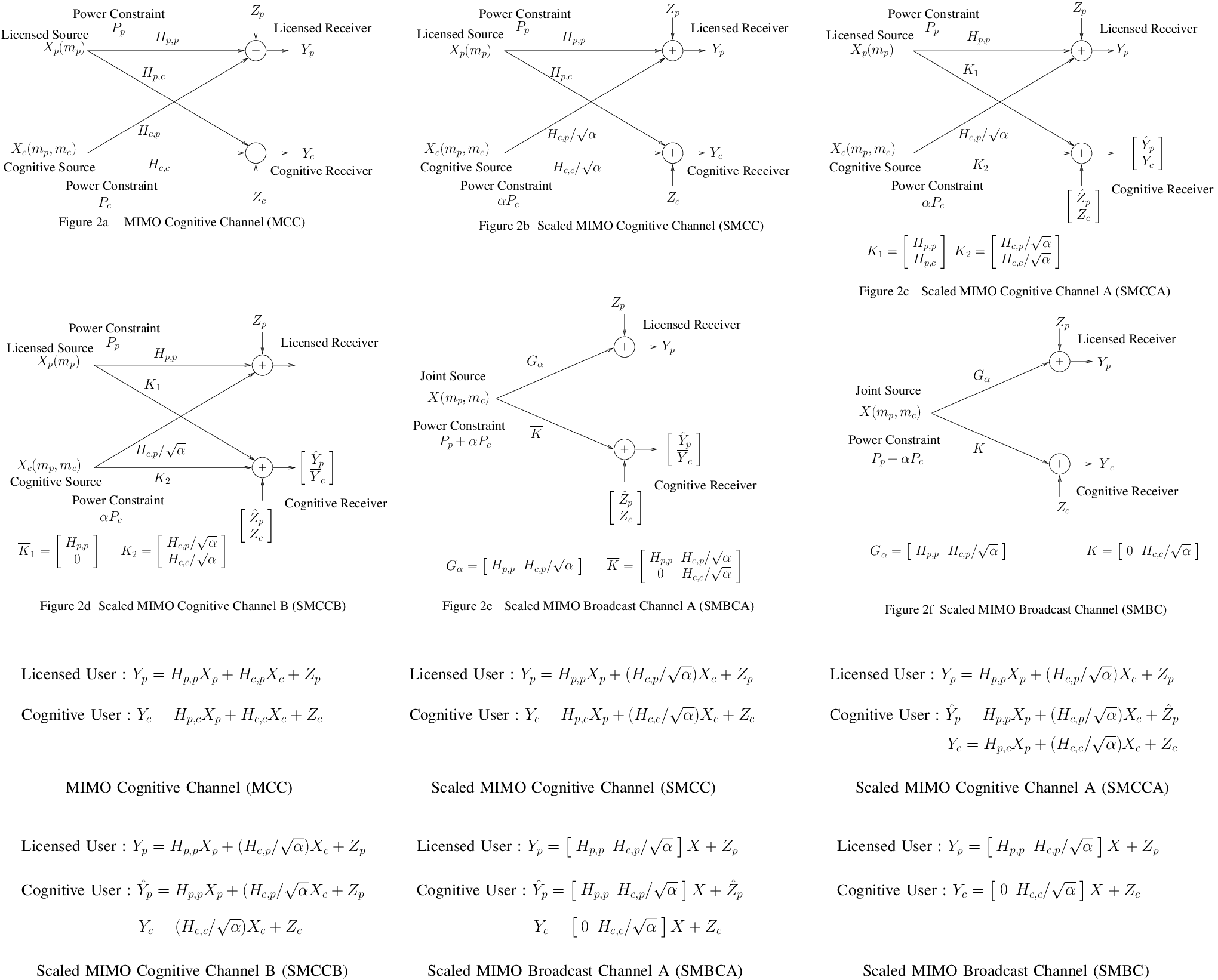
Before proving Theorem III.2, we prove the following lemmas.

Transformation 1 (MIMO Cognitive Channel (MCC) $\rightarrow$ Scaled MIMO cognitive channel) : The scaled MIMO cognitive channel is defined in Figure $2\textrm{b}$ and Figure $3$. In this transformation, the channel matrices $\mathbf{H_{c,p}}$ and $\mathbf{H_{c,c}}$ are scaled by $1/\sqrt{\alpha}$. Also, the power constraint at the cognitive transmitter is changed to $\alpha P_{c}$.

References

- [1] S. Sridharan and S. Vishwanath, “On the capacity of a class of MIMO cognitive radios,” in Proc. Information Theory Workshop (ITW) 2007, Lake Tahoe, Sept. 2007, pp. 384–389.
- [2] Federal Communications Commision, Cognitive Radio Technologies Proceeding (CRTP), ET Docket No. 03-108. http://www.fcc.gov/oet/cognitiveradio/.
- [3] J. Mitola, Cognitive Radio: An Integrated Agent Architecture for Software Defined Radio. PhD Dissertation, KTH, Stockholm, Sweeden, December 2000.
- [4] A. Ghasemi and E. Sousa, “Collaborative spectrum sensing for opportunistic access in fading environments,” in Proc. First IEEE International Symp. on New Frontiers in Dynamic Spectrum Access Networks (DySPAN), 8-11 Nov. 2005, pp. 131–136.
- [5] S. Haykin, “Cognitive radio: brain-empowered wireless communications,” IEEE Journal on selected areas in Communications, vol. 23, no. 2, pp. 201– 220, Feb 2005.
- [6] S. Srinivasa, S. Jafar, and N. Jindal, “On the capacity of the cognitive tracking channel,” in IEEE International Symposium on Information Theory, July 2006, pp. 2077–2081.
- [7] S. A. Jafar and S. Srinivasa, “Capacity limits of cognitive radio with distributed and dynamic spectral activity,” IEEE Journal on selected Areas in Communications, vol. 25, no. 3, pp. 529–537, April 2007.
- [8] S. Srinivasa and S. A. Jafar, “The throughput potential of cognitive radio: A theoretical perspective,” IEEE Communications Magazine, vol. 45, no. 5, 2007.
- [9] N. Devroye, P. Mitran, and V. Tarokh, “Achievable rates in cognitive radio channels,” IEEE Trans. Inform. Theory, vol. 52, no. 5, pp. 1813–1827, May 2006.
- [10] A. Carleial, “Interference channels,” IEEE Trans. Inform. Theory, vol. 24, no. 1, pp. 60–70, Jan. 1978.
- [11] M. Costa, “On the Gaussian interference channel,” IEEE Trans. Inform. Theory, vol. 31, no. 5, pp. 607–615, Sep 1985.
- [12] H. Sato, “The capacity of the Gaussian interference channel under strong interference (corresp.),” IEEE Trans. Inform. Theory, vol. 27, no. 6, pp. 786–788, Nov 1981.
- [13] T. Han and K. Kobayashi, “A new achievable rate region for the interference channel,” IEEE Trans. Inform. Theory, vol. 27, no. 1, pp. 49–60, Jan 1981.
- [14] I. Maric, R. Yates, and G. Kramer, “The capacity region of the strong interference channel with common information,” in Proc. Thirty-Ninth Asilomar Conference on Signals, Systems and Computers, October 28 - November 1, 2005, pp. 1737–1741.
- [15] A. Jovicic and P. Viswanath, “Cognitive radio: An information-theoretic perspective,” submitted to IEEE Trans. Inform. Theory. Preprint available at http://www.ifp.uiuc.edu/ pramodv/pubs.html.
- [16] W. Wu, S. Vishwanath, and A. Arapostathis, “On the capacity of Gaussian weak interference channels with degraded message sets,” accepted at IEEE Trans. Inform. Theory. Preprint available at http://users.ece.utexas.edu/ wwu/publications.html.
- [17] H. Weingarten, Y. Steinberg, and S. Shamai, “The capacity region of the Gaussian multiple-input multiple-output broadcast channel,” IEEE Trans. Inform. Theory, vol. 52, no. 9, pp. 3936–3964, Sept. 2006.
- [18] M. Mohseni and J. M. Cioffi, “A proof of the converse for the capacity of Gaussian MIMO broadcast channels,” in Proc. IEEE Intl. Symp. on Inform. Theory, Seattle, 2006, July 2006, pp. 881–885.
- [19] H. Weingarten, T. Liu, S. S. (Shitz), Y. Steinberg, and P. Viswanath, “The capacity region of the degraded multiple input multiple output compound broadcast channel,” submitted to IEEE Trans. Inform. Theory. Preprint available at http://www.ece.tamu.edu/ tieliu/pub/dc07.pdf.
- [20] T. M. Cover and J. A. Thomas, Elements of Information Theory. Wiley Series in Telecommunications, July 2006.
- [21] M. Costa, “Writing on dirty paper (corresp.),” IEEE Trans. Inform. Theory, vol. 29, no. 3, pp. 439–441, May 1983.
- [22] W. Yu and J. Cioffi, “Sum capacity of Gaussian vector broadcast channels,” IEEE Trans. Inform. Theory, vol. 50, no. 9, pp. 1875–1892, Sept. 2004.
- [23] S. Vishwanath, G. Kramer, S. Shamai, S. Jafar, and A. Goldsmith, “Capacity bounds for Gaussian vector broadcast channels,” in DIMACS Workshop on Signal Processing for Wireless Transmission, Rutgers, NJ, October 2002.
- [24] R. M. Dudley, Real analysis and probability. Cambridge University Press, 2002.
- [25] K. Fan, “Minimax theorems,” in Proc. Nat. Acad. Sci, 39, 1953, pp. 42–47.