$\mathbf{D}$ and $\mathbf{D_{s}}$ hadronic branching fractions at B factories

Hadronic branching fractions of $D$ and $D_{s}$ decays are used as references mode in many measurements of branching fractions of $D$ and $B$-meson decays as well. A precise measurement of such values improves our knowledge of $D$ and $B$-meson properties, and of fundamental parameters of the Standard Model, such as the magnitude of the Cabibbo-Kobayashi-Maskawa CKM matrix element.

BABAR collaboration measures the absolute branching fraction ${\cal B}(D^{0}\rightarrow K^{-}\pi^{+})$¹¹ 1 Charge conjugation is implied through the paper. using $D^{0}\rightarrow K^{-}\pi^{+}$ decays in a sample of $D^{0}$ mesons preselected by their production in $D^{*+}$ decays, obtained with partial reconstruction of the decay $\kern 1.79993pt\overline{\kern-1.79993ptB}{}^{0}\rightarrow D^{*+}X\ell^{-}\bar{\nu}_{\ell}$, with $D^{*+}\rightarrow D^{0}\pi^{+}$ Aubert:2007wn. Such measurement is extremely important because many of the past and current $D$ and $B$ branching fraction measurements are indeed systematically limited by the precision of ${\cal B}(D^{0}\rightarrow K^{-}\pi^{+})$.

A sample of partially reconstructed $B$ mesons in the channel $\kern 1.79993pt\overline{\kern-1.79993ptB}{}^{0}\rightarrow D^{*+}X\ell^{-}\bar{\nu}_{\ell}$ is selected by retaining events containing a charged lepton ($\ell=e,\,\mu$) and a low momentum pion (soft pion, $\pi^{+}_{s}$) which may arise from the decay $D^{*+}\rightarrow D^{0}\pi^{+}_{s}$. This sample of events is referred to as the “inclusive sample”.

Using conservation of momentum and energy, the invariant mass squared of the undetected neutrino is calculated as

where $E_{\mbox{\rm\small beam}}$ is half the total center-of-mass energy, $E_{\ell}~(E_{{D^{*}}})$, ${\vec{p}}_{\ell}~({\vec{p}}_{{D^{*}}})$ are the energy and momentum of the lepton (the $D^{*}$ meson) and the magnitude of the $B$ meson momentum, $p_{B}$, is considered negligible compared to $p_{\ell}$ and $p_{D^{*}}$. Figure 1 shows the ${\cal M}_{\nu}^{2}$ distribution and the results of a minimum $\chi^{2}$ fit aiming to determine the signal and background contribution. The number of signal events with ${\cal M}_{\nu}^{2}>-2$ GeV²/c⁴ results $N^{\rm incl}=(2170.64\pm 3.04(\textrm{stat})\pm 18.1(\textrm{syst}))\times 10^{3}$.

The $D^{0}\rightarrow K^{-}\pi^{+}$ decays in the inclusive sample are selected requiring events in the mass range $1.82<M_{K\pi}<1.91$ ${\mathrm{\,Ge\kern-1.00006ptV\!/}c^{2}}$ and $142.4<\Delta M<149.9$ ${\mathrm{\,Me\kern-1.00006ptV\!/}c^{2}}$ where $\Delta M=M(K^{-}\pi^{+}\pi^{+}_{s})-M(K^{-}\pi^{+})$ and $\pi^{+}_{s}$ is the slow pion from $D^{*+}$ decay. The exclusive selection yields $N^{\rm excl}=33810\pm 290$ signal events, where the error is statistical only.

The branching fraction is computed as

where $\varepsilon_{(K^{-}\pi^{+})}$ is the $D^{0}$ reconstruction efficiency as computed in the simulation, and $\zeta$ is the selection bias introduced by the partial reconstruction.

The main systematic uncertainty on $N^{\rm incl}$ and $N^{\rm excl}$ are respectively due to the non-peaking combinatorial $B\kern 1.79993pt\overline{\kern-1.79993ptB}{}$ background and the charged-track reconstruction efficiency. The complete set of systematic uncertainties is listed in Tab. 1. The absolute branching fraction of $D^{0}\rightarrow K^{-}\pi^{+}$ decay results

where the first error is statistical and the second error is systematic. This result is comparable in precision with the present world average, and it is consistent with it within two standard deviations.

The poor accuracy of the branching fraction ${\cal B}(D_{s}^{+}\rightarrow K^{+}K^{-}\pi^{+})=(5.2\pm 0.9)\%$ PDG has been a systematic limitation for some precise measurements. In particular, the recent study of the $CP$ violation in $B^{0}\rightarrow D^{(*)\pm}\pi^{\mp}$ decays is restricted by the knowledge of the ratio of two amplitudes that determine the $CP$-asymmetry belle_dp; babar_dp. The amplitude $B^{0}\rightarrow D^{(*)+}\pi^{-}$ can be calculated from the branching fraction of $B^{0}\rightarrow D_{s}^{(*)+}\pi^{-}$ decays assuming factorization. On the other hand, the factorization hypothesis can be tested by measuring the ratio of $B^{0}\rightarrow D^{(*)-}\pi^{+}$ and $B^{0}\rightarrow D^{(*)-}D_{s}^{+}$ decays. Both $\mathcal{B}(B^{0}\rightarrow D_{s}^{(*)+}\pi^{-})$ and $\mathcal{B}(B^{0}\rightarrow D^{(*)-}D_{s}^{+})$ measurements can be improved with better accuracy in $D_{s}^{+}$ absolute branching fractions.

Belle collaboration measures ${\cal B}(D_{s}^{+}\rightarrow K^{+}K^{-}\pi^{+})$ using a partial reconstruction of the process $e^{-}e^{-}\rightarrow D^{*+}_{s}D_{s1}^{-}$ Abe:2007jz. In this analysis 4-momentum conservation allows to infer the 4-momentum of the undetected part.

The process $e^{-}e^{-}\rightarrow D^{*+}_{s}D_{s1}^{-}$ is reconstructed using two different tagging procedures. The first one (denoted as the $D^{-}_{s1}$ tag) includes the full reconstruction of the $D^{-}_{s1}$ meson via $D^{-}_{s1}\rightarrow\overline{D}{}^{*}K$ decay and observation of the photon from $D^{*+}_{s}\rightarrow D^{+}_{s}\gamma$, while the $D_{s}^{+}$ is not reconstructed. The measured signal yield with the $D^{-}_{s1}$ tag is proportional to the branching fractions of the reconstructed $\overline{D}{}^{*}$ modes. In the second procedure (denoted as the $D^{*+}_{s}$ tag) a full reconstruction of $D^{*+}_{s}$ is required through $D^{*+}_{s}\rightarrow D^{+}_{s}\gamma$ and observation of the kaon from $D_{s1}^{-}\rightarrow\overline{D}{}^{*}K$, but the $\overline{D}{}^{*}$ is not reconstructed. Since the $D^{+}_{s}$ meson is reconstructed in the channel of interest, $D^{+}_{s}\rightarrow K^{+}K^{-}\pi^{+}$, the signal yield measured with the $D^{*+}_{s}$ tag is proportional to this $D^{+}_{s}$ branching fraction. The (efficiency-corrected) ratio of the two measured signal yields is equal to the ratio of well-known $\overline{D}{}^{*}$ branching fractions and the branching fraction of the $D^{+}_{s}$:

where $\mathcal{B}(\overline{D}{}^{(*)})$ is the product of $\overline{D}{}^{*}$ branching fraction and those of sub-decays.

The signal is identified by studying the mass recoiling against the reconstructed particle (or combination of particles) denoted as $X$. This recoil mass is defined as:

where $E_{X}$ and $P_{X}$ are the center-of-mass (CM) energy and momentum of X, respectively; $E_{CM}$ is the CM beam energy. A peak in the $M_{\mathrm{recoil}}$ distribution at the nominal mass of the recoil particle is expected.

Since the resolution in $M_{\mathrm{recoil}}$ is not enough to separate the relevant final states, the recoil mass difference $\Delta M_{\mathrm{recoil}}$ is used to disentangle the contribution of the different final states:

As the ratio of $D^{-}_{s1}\rightarrow\overline{D}{}^{*0}K^{-}$ and $D^{-}_{s1}\rightarrow D^{*-}K_{S}^{0}$ branching fractions is unknown, the analysis is performed for these two channels separately. Figure 2 shows the $\Delta M_{\mathrm{recoil}}(D^{-}_{s1}\gamma)$ and $\Delta M_{\mathrm{recoil}}(D^{*+}_{s}K)$ distributions used for $D_{s1}^{-}$ and $D_{s}^{*+}$ tag procedures respectively. $\Delta M_{\mathrm{recoil}}(D^{-}_{s1}\gamma)$ peaks at around $\simeq 0.14$ GeV/c${}^{2}\simeq M(D_{s}^{*})-M(D_{s})$. $\Delta M_{\mathrm{recoil}}(D^{*+}_{s}K)$ peaks at around $\simeq 0.525$ GeV/c${}^{2}\simeq M(D_{s1})-M(D^{*})$.

Using the measured signal yields $N(D^{*+}_{s})$ and $N(D^{-}_{s1})$ with $D^{*+}_{s}$ and $D^{-}_{s1}$ tags, respectively, and taking into account the efficiency ratio $\frac{\epsilon(D^{-}_{s1})}{\epsilon(D^{*+}_{s})}$, the $D^{+}_{s}$ absolute branching fraction is computed by Eq. 1 for $D^{-}_{s1}\rightarrow\overline{D}{}^{*0}K^{-}$ and $D^{-}_{s1}\rightarrow D^{*-}K_{S}^{0}$. The average value is $\mathcal{B}(D^{+}_{s}\rightarrow K^{+}K^{-}\pi^{+})=(4.0\pm 0.4(\textrm{stat})\pm 0.4(\textrm{syst})$)%.

The branching ratios of the singly Cabibbo-suppressed decays of $D^{0}$ meson are anomalous since the $D^{0}\rightarrow\pi^{-}\pi^{+}$ branching fraction is observed to be suppressed relative to the $D^{0}\rightarrow K^{-}K^{+}$ by a factor of almost three, even though the phase space for the former is larger. The branching ratios of the three-body decays PDG have larger uncertainties but do not appear to exhibit the same suppression. This motivates the current study which measures the branching ratios of $D^{0}\rightarrow\pi^{-}\pi^{+}\pi^{0}$ and $K^{-}K^{+}\pi^{0}$ with respect to the Cabbibo-favored decay $D^{0}\rightarrow K^{-}\pi^{+}\pi^{0}$. BABAR collaboration measures both branching ratios Aubert:2006xw, Belle collaboration only the decay $D^{0}\rightarrow\pi^{-}\pi^{+}\pi^{0}$ with respect to the decay $D^{0}\rightarrow K^{-}\pi^{+}\pi^{0}$ Abe:2006tv. By choosing the normalization mode $D^{0}\rightarrow K^{-}\pi^{+}\pi^{0}$, many sources of systematic uncertainty including the $\pi^{0}$ detection efficiency and uncertainty in the tracking efficiency cancel out. To reduce combinatorial backgrounds, $D^{0}$ candidates are reconstructed in decays $D^{*+}\rightarrow D^{0}\pi^{+}_{s}$ ($\pi_{s}^{+}$ is a soft, low momentum charged pion) with $D^{0}\rightarrow K^{-}\pi^{+}\pi^{0}$, $\pi^{-}\pi^{+}\pi^{0}$, and $K^{-}K^{+}\pi^{0}$, by selecting events with at least three charged tracks and a neutral pion.

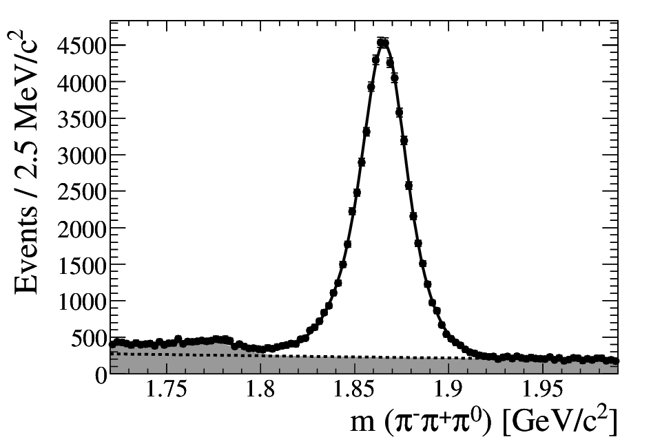
BABAR obtains the following results for the branching ratios:

while Belle obtains:

Errors are statistical and systematic, respectively. Figure 3 shows the resulting mass distributions. Reflected $K^{-}\pi^{+}\pi^{0}$ events peak in the lower (upper) sideband of $m_{\pi^{-}\pi^{+}\pi^{0}}$ ($m_{K^{-}K^{+}\pi^{0}}$).

Using the world average value for the $D^{0}\rightarrow K^{-}\pi^{+}\pi^{0}$ branching fraction PDG, the absolute branching ratios result:

To the extent that the differences in the matrix elements are only due to Cabibbo-suppression at the quark level, the ratios of the matrix elements squared for singly Cabibbo-suppressed decays to that for the Cabibbo-favored decay should be approximately $\sin^{2}\theta_{C}\approx 0.05$ and the ratio of the matrix elements squared for the two singly Cabibbo-suppressed decays should be unity. The deviations from this naive picture are less than 35% for these three-body decays. In contrast, the corresponding ratios may be calculated for the two-body decays $D^{0}\rightarrow\pi^{-}\pi^{+}$, $D^{0}\rightarrow K^{-}\pi^{+}$, and $D^{0}\rightarrow K^{-}K^{+}$. Using the world average values for two-body branching ratios PDG, the ratios of the matrix elements squared for two-body Cabibbo-suppressed decays, corresponding to Eqs. 2–5, are, respectively, $0.034\pm 0.001$, $0.111\pm 0.002$, and $3.53\pm 0.12$. Thus the naive Cabibbo-suppression model works well for three-body decays but not so well for two-body decays.

The Dalitz plot analysis is the most complete method of studying the dynamics of three-body charm decays. These decays are expected to proceed through intermediate quasi-two-body modes two and experimentally this is the observed pattern. Dalitz plot analyses can also provide new information on the resonances that contribute to observed three-body final states. In this kind of analysis the complex quantum mechanical amplitude $f$ is a coherent sum of all relevant quasi-two-body $D^{0}\rightarrow(r\rightarrow AB)C$ isobar model isobar resonances, $f=\sum_{r}a_{r}e^{i\phi_{r}}A_{r}(s)$. Here $s=m_{AB}^{2}$, and $A_{r}$ is the resonance amplitude. The isobar model is expected to fail when there are large and overlapping resonances. In such case the $\pi\pi$ $S$-wave is often parameterized through a K-matrix formalism ref:Kmatrix; ref:aitchison.