We investigate AdS/QCD duality for the two-point correlation function of the lowest dimension scalar glueball operator, in the case of the IR soft wall model. We point out the role of the boundary conditions for the bulk-to-boundary propagator in determining the gluon condensates. We show how a low energy QCD theorem can be obtained within the AdS approach, together with a gluon condensate close to the commonly accepted value and robust against perturbation of the background dilaton field.
Investigating AdS/QCD duality
through the scalar glueball correlator
pacs
11.25.Tq, 12.39.Mk,12.90.+bI Introduction
The idea that an analytic approach to QCD in the strong coupling regime is a viable possibility has recently received support from the recognition that the AdS/CFT correspondence conjecture Maldacena:1997re; Witten:1998qj; Gubser:1998 could be applied to QCD-like gauge theories Witten2:1998. In the AdS/CFT conjecture, a correspondence is supposed to exist between the supergravity limit of a Superstring/M theory defined in a holographic space of total dimension and the large limit of a maximally superconformal YM theory living on the boundary of dimension . Therefore QCD, being neither supersymmetric nor conformal, is different from the YM theories to which the AdS/CFT correspondence conjecture is applied; however, in the regime where its coupling is nearly constant and where other scales such as the quark masses can be neglected, it can be considered as an approximately conformal field theory defined on the boundary of an AdS-like holographic space. However, since confinement breaks conformal invariance, the AdS geometry needs, at least, to be modified to account for such a phenomenon. Indeed, various models have been proposed, namely introducing a maximum value (IR hard wall) of the holographic coordinate of the space interpreted as an energy scale (the IR hard wall model Polchinski:2001tt; Erlich), or considering an IR soft wall described by a background dilaton field (the IR soft wall model andreev0; son2). In both cases, a mass scale of the order is introduced and the conformal invariance is broken. With such modifications of the AdS space, studies have been carried out in order to check whether properties of QCD are reproduced in the AdS description; in particular, the meson spectroscopy and the problem of chiral symmetry breaking have been considered, following a procedure which is usually denoted as the bottom-up approach to the AdS/QCD correspondence AdSQCD; AdSQCD2; AdSQCD3; AdSQCD4; AdSQCD5; AdSQCDa; AdSQCDa1; AdSQCDa2.
The glueball sector is one of the first issues investigated through the AdS/QCD correspondence hypothesis, but mainly in the (so-called top-down) approach which attempts to extend the AdS/CFT duality to QCD-like gauge theories starting from a theory in a high dimensional space and breaking the conformal invariance and the supersymmetry, respectively, by compactification and by appropriate boundary conditions on the compactified dimensions Witten2:1998. In this way QCD is recovered as a realization of a theory in higher dimensions, and scalar and tensor glueballs have been investigated in this framework Ooguri; CsakiOoguri; demello; Zyskin; Minahan; ConstableMyers; BrowerMathur; BrowerMathur2; Babington. On the other hand, glueballs have also been studied in the bottom-up approach BoschiFilho:2002vd; BoschiFilho:2002vd2; BoschiFilhoBraga. The spectra of scalar and vector glueballs in the IR soft wall model have been determined, finding that they follow a linear Regge behaviour; moreover, the effects produced modifying the AdS geometry or the dilaton profile in the IR have also been investigated, obtaining that perturbations influence in different ways the scalar and vector glueball masses colangelo.
Further information can be obtained from the analysis of the correlation function, as done e.g. in son2; radyushkin in the meson case. In the present work, we are interested in investigating how the AdS/QCD correspondence is realized for the two-point correlation functions of scalar glueball operators. Similar analyses have been recently presented Forkel:2007ru; Beijing, but our conclusions are different, mainly as far as the values of the gluon condensates are concerned, together with their relation to the boundary conditions imposed in the holographic space.
The plan of the paper is the following. In Section II, we study the two-point correlation functions of the lowest dimension QCD operator describing the scalar glueballs, showing how the condensates are related to the bulk-to-boundary propagator defined in the holographic space. In Section III, we focus on the dimension four gluon condensate derived from an AdS/CFT argument worked out by Klebanov and Witten; this argument consists in relating the condensate to the expansion near the UV brane of the field holographically dual to the scalar glueball operator. In Section IV, we investigate how the correlation function is modified if the background dilaton field is perturbed, and the way the gluon condensate depends on such a perturbation. At the end, we present our conclusion.
II AdS/QCD duality in the glueball sector
We consider a five dimensional conformally flat spacetime (the bulk) described by the metric:
| (II.1) |
with and . The coordinates () are the usual four dimensional space-time (the boundary) coordinates, while is the fifth holographic coordinate running from zero to infinity. The metric function satisfies the condition:
| (II.2) |
to reproduce the metric close to the UV brane ; is the anti-de Sitter radius. We adopt the simplest choice compatible with this constraint:
| (II.3) |
In order to softly break the conformal invariance, we consider a background dilaton field which only depends on the holographic coordinate and vanishes at the UV brane. The large dependence of this field:
| (II.4) |
is chosen to reproduce the linear Regge behaviour of the low-lying mesons son2. The simplest choice compatible with the two constraints is
| (II.5) |
and involves the dimensionful parameter which sets the scale of QCD quantities, such as the hadron masses.
In order to investigate the glueball sector of QCD, we consider the lowest dimension QCD operator having the scalar glueball quantum numbers: ( a color index) with and conformal dimension ; is the Callan-Symanzik function. This operator is defined in the field theory living on the boundary. According to the AdS/CFT correspondence, the conformal dimension of a (-form) operator on the boundary is related to the of the dual field in the bulk by the relation Witten:1998qj:
| (II.6) |
We assume that the mass of the scalar bulk field constructed as the holographic correspondent of the operator is given by this expression. It is described by the action with the gravity and the dilaton background:
| (II.7) |
with and a dimensionful parameter. As discussed in colangelo, scalar glueball states can be identified as the normalizable modes of satisfying the equations of motion obtained from (II.7), and their mass spectrum can be obtained consequently.
In the following, we consider the two-point correlation function of the QCD operator :
| (II.8) |
In QCD, the short-distance expansion of this correlation function (obtained in our metric for ), writing and keeping the first term with ( and are, respectively, the number of colors and of active flavours; we use ), can be expressed in terms of a perturbative contribution and a series of power corrections; the result, which includes the leading order perturbative term and the power corrections up to , reads as Novikov; Novikov2; Paver; Paver2; Narison:
| (II.9) | |||||
being a renormalization scale. Eq. (II.9) involves the coefficients:
| (II.10) | |||||
and the QCD condensates of dimension four, six and eight, respectively:
| (II.11) | |||||
In addition to the short-distance expansion (in which, however, possible instanton contributions have not been considered), a Low Energy Theorem is known for the correlation function (II.8) Novikov; Novikov2:
| (II.12) |
a theorem relating the value of the correlation function at zero momentum to the dimension four gluon condensate.
Within the AdS/CFT correspondence, the correlation function (II.8) can be computed using the equivalence between the generating functional of the connected correlators in the theory and the effective action in the bulk theory. The conjecture is Witten:1998qj; Gubser:1998:
| (II.13) |
where is the effective (classical) action (II.7) of the scalar bulk field dual to the operator , for which is the source defined on the boundary. The relation between the field and its boundary value is implemented by defining the bulk-to-boundary propagator :
| (II.14) |
To achieve the condition , the bulk-to-boundary propagator must reduce to a delta function on the boundary:
| (II.15) |
In the Fourier space, the convolution (II.14) is replaced by
| (II.16) |
and involves the Fourier transforms (with respect to ) , and of , and , respectively.
Furthermore, an AdS/CFT prescription also requires the vanishing of the bulk-to-boundary propagator in the deep IR region:
| (II.17) |
we discuss this IR boundary condition in the following.
The equation of motion for the field obtained from the action (II.7) is:
| (II.18) |
where is a combination of the metric function and of the dilaton background field : . It can be written as an equation for the Fourier transform of the bulk-to-boundary propagator :
| (II.19) |
From now on, we use the dimensionless variable . The general solution of this equation can be written as:
| (II.20) |
and , constants with respect to , depend in general on . In order to determine the two independent solutions , it is convenient to solve the equation for the Bogoliubov transform of :
| (II.21) |
one obtains a one-dimensional Schrödinger-like equation colangelo:
| (II.22) |
where the derivatives act on and the potential is:
| (II.23) |
Two independent solutions and of (II.22) are:
| (II.24) |
with the Tricomi confluent hypergeometric function, and
| (II.25) |
where is the generalized Laguerre function. The function vanishes as when , while has a finite value in this limit: the UV boundary condition (II.15) imposes that in (II.20), so that the behaviour
| (II.26) |
is recovered for any value of . The low- expansion of reads:
On the other hand, the behaviour at infinity of and in (II.24) and (II.25) is very different. For diverges when , while it goes to zero for space-like four-momenta. has a strong divergence in the IR for any value of . A possible IR boundary condition in the soft wall model is that the effective action is finite in this region son2. According to this prescription, should be discarded in the calculation of (II.13) (that is, in (II.20)). However, as we discuss below, this requirement seems to produce inconsistencies in the two-point correlation function; therefore, it is worth investigating the possible role of contributions (when ) brought by to the AdS version of the correlation function. This means that the effective action in the bulk requires a regularization in the IR.
We evaluate the correlator following the AdS/CFT correspondence relation (II.13), which implies test; test2; test3; test4; test5; test6; test7; test8:
Deriving twice eq.(II.13), we obtain in terms of the variable :
so that the integration over gives the AdS representation of two-point correlation function in terms of the bulk-to-boundary propagator:
| (II.30) |
Using the solution (II.20) the expression (II.30) is singular both in the UV and in the IR. A regularization prescription consists in considering a new effective action:
| (II.31) |
where the two terms are introduced to subtract the UV (when ) and IR (when ) divergences; the first one is the usual term considered in the AdS/CFT procedure, while the second one defines the IR soft wall model: it involves , and vanishes when as in the usual procedure. The expression of the two-point correlation function reads now:
| (II.32) |
where is the Euler function, the logarithmic derivative of . This AdS representation of the two-point correlation function(II.8) should match the QCD result.
Let us consider the short-distance regime. Expanding (II.32) for :
| (II.33) | |||||
and identifying with the renormalization scale (as in csaki, since holography is related to the renormalization group verlinde; BianchiFreedmanSkenderis), we obtain:
| (II.34) | |||||
We can now compare the QCD (II.9) and the AdS (II.34) expressions: if any mismatch occurs, duality is violated. Identifying the terms in (II.9) and (II.34) we get a condition which fixes the parameter in the action (II.7):
| (II.35) |
This condition does not involve the parameter , related to the dilaton background, but is only connected to the AdS structure of the holographic space-time close to the UV boundary.
The other terms in the power expansion of the two-point correlation function involve the various gluon condensates and deserve discussion. Without the contribution of (i.e. for ), the dimension four gluon condensate obtained comparing (II.9) and (II.34), is given by:
| (II.36) |
it turns out to be negative, as also observed in Forkel:2007ru. A negative value is not compatible with current determinations of this QCD quantity Reinders; Reinders2; khodjamirian. Moreover, it would be inconsistent with a positive value obtained analyzing the two-point correlation function of vector operators Beijing, and with a determination based on computing the Wilson loop in the AdS/QCD approach in which the value GeV4 was found andreev. In both the calculations, a dilaton background field was chosen to break the conformal invariance, i.e. the IR soft wall model was used.
Another observation concerns the two-point correlation function at zero momentum. From (II.32) we obtain if :
| (II.37) |
while the Low Energy Theorem (II.12) relates to the dimension four gluon condensate. These shortcomings could cast doubts on the approach based on the IR soft wall model. However, they can be removed if the contribution of the solution in (II.20) is taken into account in the determination of the AdS version of the two-point correlation function: if we allow to contribute to the correlation function, it seems possible to recover AdS/QCD duality.
Let us discuss this point. The coefficient function is undetermined at this stage. In general, can be any function of the dimensionless ratio . If is a function having the polynomial behaviour at large space-like , namely:
| (II.38) |
its parameters can be fixed by matching the AdS expression of the two-point correlation function with the OPE expansion (II.9) of . A constant term in contributes to term involving the the dimension four gluon condensate in the power expansion, so that the gluon condensate reads:
| (II.39) |
while the other two condensates are given by
| (II.40) |
Notice that the parameter in the dilaton field sets the scale for all the condensates.
The coefficient in (II.39) can be fixed using the commonly used numerical value of the condensate Reinders; Reinders2; khodjamirian:
| (II.41) |
together with the value of the dilaton parameter from the spectrum of the mesons son2: . For one obtains . On the other hand, the AdS expressions of the dimension six (II) and dimension eight (II.40) gluon condensates are different in size (and in sign for ) from their commonly used values
| (II.42) |
(adopting in the last expression the factorization approximation). However, while the estimated uncertainty for the dimension four condensate is about , the values of the dimension six and eight gluon condensates are very uncertain, so that the difference between (II) and (II) could be attributed to the poor knowledge of the gluon vacuum matrix elements.
In the AdS expression of the two point correlator (II.34), a term involving a dimension two condensate appears, as also discussed in Forkel:2007ru; Beijing (see andreev0 in the case of the vector current). This term is missing in the QCD short-distance expansion (in general, the existence and the meaning of a dimension two condensate, which cannot be expressed as the vacuum expectation value of a local gauge invariant QCD operator, is a matter of discussion; a recent analysis of its interpretation can be found in zakharovmartina). However, this term could be removed if
| (II.43) |
and the term is included among the contact terms, an admittedly fine-tuning procedure.
Let us now consider the AdS two-point correlation function (II.32) in the full range. In Fig. 2.1 we plot for two values of : and , fixing and the scale GeV. In the time-like () region, a discrete set of poles appears according to the spectral relation ( is an integer)
| (II.44) |
obtained in colangelo. The residues
| (II.45) |
related to the matrix elements , coincide with the result obtained in Forkel:2007ru. The structure in poles in (II.32) is due to the Euler function . It does not depend on , but it comes from the solution in (II.20) which can be written according to the spectral representation Beijing:
| (II.46) |
where are the normalizable modes computed in colangelo:
| (II.47) |
Nevertheless, the expression (II.46) in terms of pole masses and residues does not define unambiguously the general solution (II.20) which can indeed contain extra regular terms in , for example if is a polynomial as in (II.38); however, these terms can affect the power expansion and the value of the condensates, as discussed, e.g., in Novikov; Novikov2.
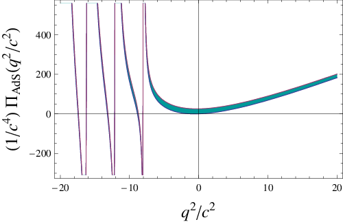
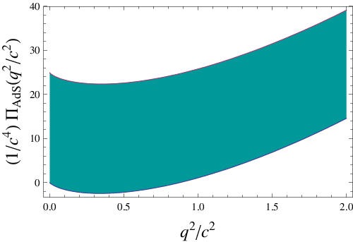
In the space-like region () the behaviour of is smooth. In the region close to , as shown in Fig. 2.1 (right panel), one finds from (II.32):
| (II.48) |
Calling and using (II.39) we have:
| (II.49) |
an expression similar to the Low Energy Theorem (II.12). For a constant coefficient function , it is possible to constrain the value of imposing that (II.49) and (II.12) coincide:
| (II.50) |
Using this expression in (II.39), together with we find:
| (II.51) |
while for we have:
| (II.52) |
These values are smaller but close to (II.41) and compatible with the result obtained studying the Wilson loop andreev which indicates that the solution (II.25) could play a role in reconstructing a bulk-to-boundary propagator which implements the AdS/QCD duality in this case.
We close this Section observing that it is possible to investigate the role of the two solutions analogous to (II.20) in the two-point correlation function of the meson operators son2; Beijing , studying duality between the QCD and the AdS expressions of the correlation function. The perturbative term is reproduced: it does not depend on the parameter . The dimension four gluon condensate is positive Beijing, and the effect of including the subleading solution with a constant coefficient function only consists in modifying the dimension two condensate. In this case, however, the contribution of the dimension six condensate in the power expansion of is not reproduced in if is a polynomial in .
III Gluon condensate from an AdS/CFT argument applied to the glueball sector
It is interesting to consider the dimension four gluon condensate from another viewpoint. From AdS/CFT correspondence, a scalar bulk field is required to satisfy the UV boundary condition Klebanov:
| (III.1) |
is the dimension of the boundary space-time and is the conformal dimension of the operator associated to the source field . can be considered as a physical fluctuation and is argued to be related to the vacuum expectation value of the corresponding CFT operator, as obtained by Klebanov and Witten:
| (III.2) |
In our case, and eq.(III.1) becomes:
| (III.3) |
with
| (III.4) |
Following this AdS/CFT guideline, let us see if it is possible to recover the four dimension gluon condensate. In our case, in the Fourier space, this term appears in the bulk-to-boundary propagator (II), considering the whole contribution proportional to , taking the limit and keeping the piece independent of . After having properly renormalized the bulk field in (II.7) by absorbing the factor, we get:
| (III.5) |
The expression is identical to (II.39) but for a overall factor which could be related to the normalization of the term, a shortcoming deserving further investigations in order to gain a deeper understanding of the AdS/QCD duality. Notice that, with respect to AdS/CFT, the new aspect is the presence of the dimensionful parameter , so that terms as , , etc., appear in the expansion (III.1).
IV AdS/QCD duality in a deformed AdS-dilaton background
The form of the dilaton background field (II.5) is the simplest choice allowing to fulfill the constraints (II.4) and . Other expressions could be used, and indeed in ref.colangelo we investigated the effects on the glueball spectrum of a perturbation of the dilaton field which, instead of being given by eq.(II.5), involves an additional term which does not spoil the UV () and IR () behaviour:
| (IV.1) |
with a small dimensionless parameter. This new background field does not sensibly modify the Regge behaviour of the spectrum.
The equation of motion (II.18) for the bulk-to-boundary propagator, with the deformed AdS-dilaton background, takes the form:
| (IV.2) |
where
| (IV.3) | |||||
| (IV.4) |
The Frobenius method allows to obtain the new bulk-to-boundary propagator:
| (IV.5) |
as an expansion of the solutions in ; , with a real parameter, and given by:
| (IV.6) |
The coefficients in (IV) read:
| (IV.7) | |||||
and
| (IV.8) | |||||
It is worth pointing out that the two expansions obtained by this method do not correspond to the expansions, respectively, of the functions and in (II.24) and (II.25) when , but represent solutions in a different basis of functions.
The AdS two-point correlation function:
| (IV.9) |
takes the form in the large space-like limit (regularizing the contribution):
| (IV.10) | |||||
The logarithmic term in the perturbative contribution remains unchanged, and the parameter is still given by eq.(II.35). This is an understandable result: the dilaton does not modify the AdS dynamics in the (UV) regime, therefore duality with the perturbative QCD term is not affected by its perturbations.
On the contrary, the other terms are modified, but the effect of perturbations on the condensate is quadratic in . The dimension four gluon condensate is now given by
| (IV.11) |
The perturbations occur at , showing that the condensate is robust against perturbations of the dilaton field of the form (IV.1).
V Conclusions
We have investigated duality between the QCD and the AdS description of the two-point correlation functions of the scalar glueballs, finding that the QCD short-distance expansion can be recovered in the AdS approach; however, the condensates depend on a condition which, in addition to the normalization at , fixes the bulk-to-boundary propagator in the IR. We have obtained the spectra and decay constants of the scalar glueballs. Moreover, we have investigated how AdS can reproduce a low energy QCD theorem for the two-point scalar glueball correlation function. Assuming a particular form of the coefficient function which reproduces the low-energy theorem, we have determined the dimension four gluon condensate, which turns out to be positive, close to the commonly accepted value and compatible with the AdS/QCD results obtained investigating the two-point vector correlation function and the Wilson loop.
Acknowledgements.
We are indebted to H. Forkel for comments. One of us (FDF) thanks Prof. A.J.Buras and the T31 group at Technische Universität, München. This work was supported in part by the EU contract No. MRTN-CT-2006-035482, "FLAVIAnet".References
- (1) J. M. Maldacena, Adv. Theor. Math. Phys. 2, 231 (1998) [Int. J. Theor. Phys. 38, 1113 (1999)].
- (2) E. Witten, Adv. Theor. Math. Phys. 2, 253 (1998);
- (3) S. S. Gubser, I. R. Klebanov and A. M. Polyakov, Phys. Lett. B 428, 105 (1998).
- (4) E. Witten, Adv. Theor. Math. Phys. 2, 505 (1998).
- (5) J. Polchinski and M. J. Strassler, Phys. Rev. Lett. 88, 031601 (2002);
- (6) J. Erlich, E. Katz, D. T. Son and M. A. Stephanov, Phys. Rev. Lett. 95, 261602 (2005).
- (7) O. Andreev, Phys. Rev. D 73, 107901 (2006).
- (8) A. Karch, E. Katz, D. T. Son and M. A. Stephanov, Phys. Rev. D 74, 015005 (2006).
- (9) S. J. Brodsky and G. F. de Teramond, Phys. Lett. B 582, 211 (2004).
- (10) S. J. Brodsky and G. F. de Teramond, Phys. Rev. Lett. 94, 201601 (2005).
- (11) S. J. Brodsky and G. F. de Teramond, Phys. Rev. Lett. 96, 201601 (2006).
- (12) L. Da Rold and A. Pomarol, Nucl. Phys. B 721, 79 (2005);
- (13) O. Andreev and V. I. Zakharov, Phys. Rev. D 74, 025023 (2006).
- (14) U. Gursoy, E. Kiritsis and F. Nitti, JHEP 0802, 019 (2008).
- (15) T. Huang and F. Zuo, Eur. Phys. J. C 56, 75 (2008)
- (16) H. J. Kwee and R. F. Lebed, JHEP 0801, 027 (2008).
- (17) D. J. Gross and H. Ooguri, Phys. Rev. D 58, 106002 (1998);
- (18) C. Csaki, H. Ooguri, Y. Oz and J. Terning, JHEP 9901, 017 (1999);
- (19) R. de Mello Koch, A. Jevicki, M. Mihailescu and J. P. Nunes, Phys. Rev. D 58, 105009 (1998);
- (20) M. Zyskin, Phys. Lett. B 439, 373 (1998).
- (21) J. A. Minahan, JHEP 9901, 020 (1999).
- (22) N. R. Constable and R. C. Myers, JHEP 9910, 037 (1999).
- (23) R. C. Brower, S. D. Mathur and C. I. Tan, Nucl. Phys. B 574, 219 (2000).
- (24) R. C. Brower, S. D. Mathur and C. I. Tan, Nucl. Phys. B 587, 249 (2000).
- (25) J. Babington, D. E. Crooks and N. J. Evans, Phys. Rev. D 67, 066007 (2003).
- (26) H. Boschi-Filho and N. R. F. Braga, JHEP 0305, 009 (2003).
- (27) H. Boschi-Filho and N. R. F. Braga, Eur. Phys. J. C 32, 529 (2004).
- (28) H. Boschi-Filho, N. R. F. Braga and H. L. Carrion, Phys. Rev. D 73, 047901 (2006).
- (29) P. Colangelo, F. De Fazio, F. Jugeau and S. Nicotri, Phys. Lett. B 652, 73 (2007).
- (30) H. R. Grigoryan and A. V. Radyushkin, Phys. Rev. D 76, 095007 (2007).
- (31) H. Forkel, Phys. Rev. D 78, 025001 (2008)
- (32) F. Zuo and T. Huang, arXiv:0801.1172 [hep-ph].
- (33) V. A. Novikov, M. A. Shifman, A. I. Vainshtein and V. I. Zakharov, Nucl. Phys. B 165, 67 (1980).
- (34) V. A. Novikov, M. A. Shifman, A. I. Vainshtein and V. I. Zakharov, Nucl. Phys. B 191, 301 (1981).
- (35) P. Pascual and R. Tarrach, Phys. Lett. B 113, 495 (1982).
- (36) C. A. Dominguez and N. Paver, Z. Phys. C 31, 591 (1986).
- (37) S. Narison, Nucl. Phys. B 509, 312 (1998).
- (38) D. Z. Freedman, S. D. Mathur, A. Matusis and L. Rastelli, Nucl. Phys. B 546, 96 (1999).
- (39) V. Balasubramanian, P. Kraus and A. E. Lawrence, Phys. Rev. D 59, 046003 (1999).
- (40) V. Balasubramanian, P. Kraus, A. E. Lawrence and S. P. Trivedi, Phys. Rev. D 59, 104021 (1999).
- (41) G. E. Arutyunov and S. A. Frolov, Nucl. Phys. B 544, 576 (1999).
- (42) G. E. Arutyunov and S. A. Frolov, JHEP 0004, 017 (2000).
- (43) W. Mueck and K. S. Viswanathan, JHEP 9907, 018 (1999).
- (44) W. Mueck and K. S. Viswanathan, Phys. Rev. D 60, 081901 (1999).
- (45) E. D’Hoker and D. Z. Freedman, arXiv:hep-th/0201253.
- (46) C. Csaki and M. Reece, JHEP 0705, 062 (2007).
- (47) J. de Boer, E. P. Verlinde and H. L. Verlinde, JHEP 0008, 003 (2000);
- (48) M. Bianchi, D. Z. Freedman and K. Skenderis, Nucl. Phys. B 631, 159 (2002).
- (49) M. A. Shifman, A. I. Vainshtein and V. I. Zakharov, Nucl. Phys. B 147, 385 (1979);
- (50) L. J. Reinders, H. Rubinstein and S. Yazaki, Phys. Rep. 127, 1-97 (1985).
- (51) P. Colangelo and A. Khodjamirian, in ’At the Frontier of Particle Physics / Handbook of QCD’, ed. by M. Shifman (World Scientific, Singapore, 2001) vol. 3* 1495-1576.
- (52) O. Andreev and V. I. Zakharov, Phys. Rev. D 76, 047705 (2007).
- (53) V. I. Zakharov, “Old problems of QCD phenomenology in view of AdS/QCD correspondence,” Proceedings of QCD@Work 2007, International Workshop on Quantum Chromodynamics Theory and Experiment, Martina Franca, Italy, 16-20 June 2007, P. Colangelo et al. editors, AIP Conf. Proc. 964, 143 (2007).
- (54) I. R. Klebanov and E. Witten, Nucl. Phys. B 556, 89 (1999).