Non-trivalent graph cocycle and cohomology of the long knot spaceThanks: The author is supported by 21st century COE program at Graduate School of Mathematical Sciences, University of Tokyo

The author expresses his appreciation to Alberto Cattaneo, Ryan Budney, Fred Cohen, Toshitake Kohno, Paolo Salvatore and Victor Turchin for reading the draft of this paper and giving him many useful advices. He is also grateful to Ismar Volić for pointing out a mistake in the previous version of this paper. The author noticed a result of Longoni by virtue of an information in Dai Tamaki’s website (which is written in Japanese).

In this paper we always assume $n>3$ is odd.

The space $\widetilde{\mathcal{K}}_{n}$ defined as above was denoted by $EC(1,B^{n-1})$ in [3]. We define the framed long knots as in the cylinder, because it becomes easier in this setting to define the little disks action.

We have a forgetting map $r:\widetilde{\mathcal{K}}_{n}\to\mathcal{K}_{n}$ defined by

The subgroup $\bigoplus_{k\geq 0}H_{(n-3)k}(\mathcal{K}_{n})$ is known to be non-trivial [5, 9, 16, 17] since it contains the subalgebra isomorphic to the algebra $\mathcal{A}$ of chord diagrams modulo 4-term and 1-term relations, and few other cycles are known. The purpose of this paper is to find another (co)cycle which does not come from any chord diagrams.

Here we explain two examples of cycles made from chord diagrams, namely, $e\in H_{n-3}(\widetilde{\mathcal{K}}_{n})$ and $v_{2}\in H_{2(n-3)}(\mathcal{K}_{n})$ which we will use later. For more general treatment, see [5, 9, 12, 17].

Here we recall the operad action of $\mathcal{B}_{2}$ on $\widetilde{\mathcal{K}}_{n}$ defined in [3], that is, the “associative” maps

Given $b=(b_{1},\dots,b_{k})\in\mathcal{B}_{2}(k)$, consider the projections

There are the little 1-balls $l_{j}(t)=a_{j}t+b_{j}$ such that $l_{j}([-1,1])=I_{j}$, $1\leq j\leq k$ ($l_{1},\dots,l_{k}$ are not necessarily disjoint mutually).

A little 1-ball $l:[-1,1]\to[-1,1]$, $l(t)=at+b$, extends to a diffeomorphism $\tilde{l}:\mathbb{R}^{1}\to\mathbb{R}^{1}$ in an obvious way, and determines a map

For any little $2$-ball $b$, define the number $t_{b}\in[-1,1]$ by

With these notations in hand, we can define the map $\kappa$ by

where $\sigma\in\mathfrak{S}_{k}$ is such that $t_{b_{\sigma(1)}}\leq\dots\leq t_{b_{\sigma(k)}}$.

In particular, $\kappa(2):\mathcal{B}_{2}(2)\times(\widetilde{\mathcal{K}}_{n})^{2}\to\widetilde{\mathcal{K}}_{n}$ is ‘pushing one long knot $f_{1}$ through another long knot $f_{2}$, afterward pushing $f_{2}$ through $f_{1}$’ (see Figure 5 and Figures 2, 5, 7 in [3]).

The space $\mathcal{B}_{2}(2)$ is homotopy equivalent to $S^{1}$. The map $\kappa(2):\mathcal{B}_{2}(2)\times(\widetilde{\mathcal{K}}_{n})^{2}\to\widetilde{\mathcal{K}}_{n}$ induces on homology two products

corresponding to generators of $H_{p}(\mathcal{B}_{2}(2))$, $p=0,1$, respectively. The former product is equal to that induced by the connecting sum. The latter $\lambda$ is called Browder operation and is a 1-Poisson bracket, that is, a Lie bracket of degree one, satisfying the Leibniz rule (see [6]).

Our attention will be paid to the element $\lambda(e,v_{2})\in H_{3n-8}(\widetilde{\mathcal{K}}_{n})$ or its image $\Lambda:=r_{*}\lambda(e,v_{2})\in H_{3n-8}(\mathcal{K}_{n})$ via the forgetful map $r:\widetilde{\mathcal{K}}_{n}\to\mathcal{K}_{n}$. For definiteness, we choose a map

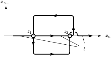
representing $v_{2}$ by resolving an immersion $f$ (Figure 6). Most part of the embedding lies in the $x_{n-1}x_{n}$-plane. The self-intersections to be resolved are $z_{i}=f(\xi_{i})=f(\xi_{i+2})$, $\xi_{i}<\xi_{i+2}$, $i=1,2$. The vectors $u_{i}\in S^{n-3}$, $i=1,2$ (which are normal to $x_{n-1}x_{n}$-plane) produce the resolutions of the self-intersections $z_{i}$, respectively. The segments $l$ are included in the $x_{n}$-axis.

Given the ‘trivial frame,’ $v$ can represent the cycle $[v]=v_{2}\in H_{2(n-3)}(\widetilde{\mathcal{K}}_{n})$.

Then the representative $\lambda(e,v)$ is the family of embeddings defined by ‘pushing $e$ through $v$, afterward pushing $v$ through $e$.’

We want to know the representative of $\Lambda=r_{*}(\lambda(e,v_{2}))\in H_{3n-8}(\mathcal{K}_{n})$. $\Lambda$ is obtained from $\lambda(e,v)$ by forgetting the frame. When $e$ goes through $v$, the frame of $v$ ‘near’ $e$ would be agitated. But this phenomenon disappears after forgetting the frame via $r:\widetilde{\mathcal{K}}_{n}\to\mathcal{K}_{n}$. In contrast, when $v$ passes through $e$, the whole embedding $v$ ‘rotates’ around $x_{n}$-axis via the frame $e$, and this phenomenon does not disappear even if we forget the frame. Thus $\Lambda$ is represented by ‘$v$ rotated by $e$.’

More precisely, if we think of $SO(n-1)$ as a subgroup of $SO(n)$ fixing the $x_{n}$-axis, then $\Lambda$ can be represented by the map

where $p:\mathbb{R}^{n}\to\mathbb{R}^{1}$ is the projection $(x_{1},\dots,x_{n})\mapsto x_{n}$. Thus $\Lambda([s,u_{0}],u_{1},u_{2})$ is a long knot $v(u_{1},u_{2})$ with its intersection with $p^{-1}(a)$ being rotated around the $x_{n}$-axis by the frame $e[2s+a,u_{0}]\in SO(n-1)$, $\lvert{a}\rvert\leq 1$.

The cycle $\Lambda$ has a simpler description; for $0\leq\tau\leq 1$, define

then $\Lambda^{\prime}_{\tau}$ is well-defined for any $\tau\in[0,1]$, $\Lambda_{0}^{\prime}=\Lambda$ and

Below we rewrite $\Lambda:=[\Lambda^{\prime}_{1}]\in H_{3n-8}(\mathcal{K}_{n})$. This $\Lambda$ is $v(u_{1},u_{2})$ rotated all together by $e[s,u_{0}]$.

An example of a graph is shown in Figure 7.

Consider the vector space spanned by the graphs with $\mathrm{ord}\,\Gamma=k$ and $\deg\Gamma=l$ modulo the subspace generated by

1. (1)

   $\Gamma$, two vertices of which are joined by more than one edges,

2. (2)

   $\Gamma$ with a small loop whose endpoint is not a free vertex, and

3. (3)

   $\Gamma^{\prime}-(-1)^{\mathrm{sign}\,\sigma}\Gamma$, here $\Gamma^{\prime}$ is obtained from $\Gamma$ by a permutation $\sigma$ which permutes the labels of the vertices (so that the labels of the interval vertices are less than those of free vertices) or reversing the orientations of the edges.

We denote the quotient space by $\mathcal{D}^{k,l}$.

The differential $\delta:\mathcal{D}^{k,l}\to\mathcal{D}^{k,l+1}$ is defined as follows. For any graph $\Gamma$, $\delta\Gamma$ is the signed sum of graphs obtained by contracting, one at a time, the edges one of whose endpoint is not interval, and the arcs, portions of the special line bounded by two consecutive interval vertices.

Determining the labels and signs of the graphs after contraction (see [5]), we can show the following directly by definition.

Below we will associate a differential form of $\mathcal{K}_{n}$ with a given graph $\Gamma$.

We denote the configuration space by

For any $N$, the Gauss maps $\varphi_{ij}:\mathrm{Conf}\,(\mathbb{R}^{N},m)\to S^{N-1}$ ($1\leq i\neq j\leq m$) are defined by

We use the compactifications of the configuration spaces.

Roughly speaking, the points in $\mathrm{Conf}\,[M,m]$ may ‘collide with each other,’ but in such cases, information of the directions of the collision must be recorded.

Let $\Gamma\in\mathcal{D}^{k,l}$ be a graph with $e$ edges, $v_{i}$ interval vertices and $v_{f}$ free vertices (hence $e-v_{f}=k$, $2e-3v_{f}-v_{i}=l$). Consider the following pull-back square:

here $\mathrm{Conf}_{0}[\mathbb{R}^{1},m]$ is a connected component corresponding to $t_{1}\leq t_{2}\leq\dots\leq t_{m}$ and, on the interior, $ev$ and $\pi_{*}$ are defined by

$\mathrm{Conf}\,[\mathbb{R}^{n};v_{i},v_{f}]$ is the space of pairs $((x_{1},\dots,x_{v_{i}+v_{f}}),f)$, where

and $f\in\mathcal{K}_{n}$, with $x_{1},\dots,x_{v_{i}}$ on the knot $f$.

With an edge (or a small loop) $\overrightarrow{ij}$ of $\Gamma$, we assign a differential form $\theta_{ij}\in\Omega^{n-1}(\mathrm{Conf}\,[\mathbb{R}^{n};v_{i},v_{f}])$ defined by

here, for $1\leq i\leq v_{i}$,

We define a form $\theta_{\Gamma}\in\Omega^{(n-1)e}(\mathrm{Conf}\,[\mathbb{R}^{n};v_{i},v_{f}])$ by

Note that this form is defined independently of the order of $\theta_{ij}$’s, since they are even forms.

Integrating this form along the fiber of

we obtain a differential form

This integral actually converges since we compactify the configuration spaces. The degree of the form $I(\Gamma)$ is

Thus we have a map

Notice that a chord diagram with $k$ chords is thought of as in $\mathcal{D}^{k,0}$ if some orientation of edges are given to $\Gamma$. The chord diagram has $e=k$ edges, $v_{i}=2k$ interval vertices, and no free vertices ($v_{f}=0$).

The proof of the following is a combinatorial one.

For example, a cochain $\Gamma_{1}-\Gamma_{2}$ given in Example 3.4 contains a chord diagram $\Gamma_{1}$, and there is no isolated chord.

Let $\Gamma=\sum_{i}a_{i}\Gamma_{i}\in\mathcal{D}^{k,0}$ be a non-zero cocycle, and suppose $\Gamma_{1}$ is a chord diagram with $a_{1}\neq 0$. Then $I(\Gamma)\in H^{(n-3)k}_{DR}(\mathcal{K}_{n})$ turns out to be not zero by the following theorem.

A detailed proof can be found in [5]. Here, as an example, we compute $\langle{I(\Gamma)},\,{v_{2}}\rangle$ where $\Gamma=\Gamma_{1}-\Gamma_{2}$ is a cocycle given in Example 3.4 (notice that the cycle $v_{2}$ is equal to $\alpha(\Gamma_{1})$). This computation is easily generalized to prove Theorem 3.8, and gives us a lot of useful suggestions for the proof of our main theorem.

Let $v_{i}$ and $v_{f}$ the numbers of interval and free vertices of the graph $\Gamma_{j}$, $j=1,2$ (if $j=1$, then $v_{i}=4$ and $v_{f}=0$; if $j=2$, then $v_{i}=3$, $v_{f}=1$). Consider the following pull-back square;

Then

and in this case the integrands are

Recall that the immersion $f$ has the transversal self-intersections $z_{i}=f(\xi_{i})=f(\xi_{i+2})$, $\xi_{1}<\xi_{2}<\xi_{3}<\xi_{4}$. Let $\varepsilon_{i}>0$ ($i=1,2$) be sufficiently small numbers appeared in the definition of the resolution of $f$ (§2.2) and define the subspace $C=C_{\varepsilon}\subset\mathrm{Conf}_{0}[\mathbb{R}^{1},v_{i}]$ by

Notice that the complementary set $\mathrm{Conf}_{0}[\mathbb{R}^{1},v_{i}]\setminus C$ is the set of configurations such that there is at least one $t_{m}$ near $\xi_{i}$, $1\leq i\leq 4$.

Write $\omega^{(j)}:=\tilde{p}_{*}\beta^{*}\theta_{\Gamma_{j}}$ and

References

• [1] S. Axelrod and I. M. Singer, Chern-Simons perturbation theory II, J. Diff. Geom. 39 (1994), 173–213.
• [2] R. Bott and C. Taubes, On the self-linking of knots, J. Math. Phys. 35 (1994), no. 10, 5247–5287.
• [3] R. Budney, Little cubes and long knots, Topology 46 (2007), 1–27.
• [4] R. Budney and F. R. Cohen, On the homology of the space of knots, math.GT/0504206.
• [5] A. Cattaneo, P. Cotta-Ramusino, and R. Longoni, Configuration spaces and Vassiliev classes in any dimensions, Algebr. Geom. Topol. 2 (2002), 949–1000.
• [6] F. R. Cohen, The homology of 𝒞n+1\mathcal{C}_{n+1}-space, n≥0n\geq 0, The Homology of Iterated Loop Spaces, Lecture Notes in Math., vol. 533, Springer, 1976, pp. 207–351.
• [7] T. Kohno, Vassiliev invariants and de Rham complex on the space of knots, Contemp. Math., vol. 179, Amer. Math. Soc., Providence, RI.
• [8] P. Lambrechts, V. Turchin, and I. Volić, The rational homology of spaces of knots in codimension >2>2, math.AT/0703649.
• [9] R. Longoni, Nontrivial classes in H∗​(Imb​(S1,ℝn))H^{*}(\text{Imb}\,(S^{1},\mathbb{R}^{n})) from nontrivalent graph cocycles, Int. J. Geom. Methods Mod. Phys. 1 (2004), no. 5, 639–650.
• [10] P. May, The geometry of iterated loop spaces, Lecture Notes in Math., vol. 271, Springer Verlag, 1972.
• [11] J. McClure and J. Smith, Cosimplicial objects and little nn-cubes I, Amer. J. Math. 126 (2004), no. 5, 1109–1153.
• [12] K. Sakai, Poisson structures on the homology of the space of knots, to appear in Geometry and Topology Monographs.
• [13] P. Salvatore, Knots, operads and double loop spaces, Int. J. Res. Not. (2006).
• [14] D. Sinha, The topology of spaces of knots, math.AT/0202287.
• [15] by same author, Manifold theoretic compactifications of configuration spaces, Selecta Math. (new ser.) 10 (2004), no. 3, 391–428.
• [16] by same author, Operads and knot spaces, J. Amer. Math. Soc. 19 (2006), no. 2, 461–486.
• [17] V. Tourtchine (Turchin), On the other side of the bialgebra of chord diagrams, J. Knot Theory Ramifications 16 (2007), no. 5, 575–629.
• [18] I. Volić, A survey of Bott-Taubes Integration, J. Knot Theory Ramifications 16, no. 1, 1–42.