Optimization of Information Rate Upper and Lower Bounds for Channels with Memory¹¹footnotemark: 1 ^∗ Thanks: ^∗Submitted to IEEE Transactions on Information Theory, November 24, 2007. Preliminary results of this paper were presented at the IEEE International Symposium on Information Theory (ISIT), Nice, France, June 2007. The work of Parastoo Sadeghi was partly supported under Australian Research Council’s Discovery Projects funding scheme (project number DP0773898).

Parastoo Sadeghi²²footnotemark: 2 Thanks: $ˆ†$Parastoo Sadeghi (contact author) and Ramtin Shams are with the Department of Information Engineering, Research School of Information Sciences and Engineering, The Australian National University, Canberra 0200 ACT, Australia. Emails: parastoo.sadeghi@anu.edu.au; ramtin.shams@anu.edu.au Pascal O. Vontobel³³footnotemark: 3 Thanks: $ˆ‡$Pascal O.˜Vontobel is with Hewlett-Packard Laboratories, Palo Alto, CA 94304, USA. Email: pascal.vontobel@ieee.org Ramtin Shams⁴⁴footnotemark: 4

Abstract

We consider the problem of minimizing upper bounds and maximizing lower bounds on information rates of stationary and ergodic discrete-time channels with memory. The channels we consider can have a finite number of states, such as partial response channels, or they can have an infinite state-space, such as time-varying fading channels.

We optimize recently-proposed information rate bounds for such channels, which make use of auxiliary finite-state machine channels (FSMCs). Our main contribution in this paper is to provide iterative expectation-maximization (EM) type algorithms to optimize the parameters of the auxiliary FSMC to tighten these bounds. We provide an explicit, iterative algorithm that improves the upper bound at each iteration. We also provide an effective method for iteratively optimizing the lower bound. To demonstrate the effectiveness of our algorithms, we provide several examples of partial response and fading channels, where the proposed optimization techniques significantly tighten the initial upper and lower bounds. Finally, we compare our results with an improved variation of the simplex local optimization algorithm, called Soblex. This comparison shows that our proposed algorithms are superior to the Soblex method, both in terms of robustness in finding the tightest bounds and in computational efficiency.

Interestingly, from a channel coding/decoding perspective, optimizing the lower bound is related to increasing the achievable mismatched information rate, i.e., the information rate of a communication system where the decoder at the receiver is matched to the auxiliary channel, and not to the original channel.

Keywords — Finite-state machine channels, information rate, lower bounds, mismatched decoding, optimization, stationary and ergodic channels, upper bounds.

I Introduction

I-A Motivation and Background

Channels with memory are common in practical communication systems. The partial response channel is an important example of a channel with memory with applications in magnetic and optical recording, as well as in communications over band-limited channels with inter-symbol interference (ISI) [1]. The time-varying multipath fading channel in wireless communication systems is another example of a channel with memory [2]. Although the information rate of such channels is formulated (we assume them to be stationary and ergodic), the direct computation of the information rate (under the assumption of no channel state information (CSI) at the receiver or the transmitter) has remained an open problem [3].

Partial response channels can be closely modeled by finite-state machine channels (FSMCs) [4]. Stochastic and numerical strategies have been proposed in the literature for efficient computation of information rates for FSMCs [5, 3, 6, 7]. The numerical estimate of the information rate converges under mild conditions with probability one to the true value when the length of the channel input and output sequences goes to infinity. Upper and lower bounds on the capacity of FSMCs have been proposed in [8, 9, 10], where the upper bound in [8] is based on Lagrange duality, the upper bound in [9] is based on the FSMC feedback capacity, and the lower bound in [10] is obtained by numerically optimizing the parameters of the Markov input source to the channel. From a practical viewpoint, information rates, the capacity, and the capacity-achieving input distribution of FSMCs with not too many states is numerically computable. However, for more complex partial response channels with longer memories, the large number of states in the FSMC prohibits efficient computation of information rates. Physical multipath fading channels are channels with an infinite (continuous-valued) state space. Therefore, direct application of the techniques in [5, 3, 6, 7] for computing information rates for fading channels is not possible.

For the case of stationary and ergodic channels with memory that are non-finite-state or where the number of states is large, we would still like to efficiently (stochastically) compute upper and lower bounds on the information rate. Such upper and lower bounds were proposed in [11, 3] based on the introduction of an auxiliary FSMC. The bounds are generally applicable to finite-state and non-finite-state channels with memory that are stationary and ergodic. The lower bound in [11, 3] is a special case of the generalized mutual information (GMI) lower bound for mismatched decoding [12]. In other words, the lower bound signifies achievable information rates when the receiver is equipped with a decoding algorithm which is matched to the auxiliary channel model and hence, usually mismatched to the original channel (over which the actual communication takes place).

The maximum number of states and branches in the auxiliary FSMC model is dictated by the computational complexity of running the Bahl-Cocke-Jelinek-Raviv (BCJR) algorithm [13] or the mismatched decoding budget. The number of auxiliary FSMC states and branches, along with the FSMC state transition and output probabilities, affect the tightness of the bounds. Therefore, for a given auxiliary FSMC trellis section, it is desirable to optimize the remaining auxiliary FSMC parameters to obtain the tightest information rate upper and lower bounds, which is the topic of this paper.

I-B Contributions and Organization

In this paper, we optimize the parameters of the auxiliary FSMC model in order to tighten the information rate upper and lower bounds that were introduced in [11, 3] for channels with memory. Actually, the lower bounds that we use in the present paper are slightly more general than the lower bounds in [11, 3]. They are also more general than the lower bounds that were optimized in the preliminary version [14] of this paper.

The original and auxiliary channels are reviewed in Section II and the information rate bounds under consideration are reviewed in Section III. In our approach, we assume that we are given a fixed trellis section of an auxiliary FSMC and that we optimize its remaining parameters (the state transition and output probabilities). The general optimization idea is shown in Section IV. Briefly speaking, we replace the optimization of a function by a succession of surrogate-function optimizations, an approach that can be seen as as a variation of the expectation-maximization (EM) algorithm [15].

Five main contributions of the paper are summarized as follows.

1.

In Section V, we propose an iterative procedure for the minimization of the upper bound. For this purpose, we devise an easily optimizable surrogate function. We establish that this surrogate function is never below the original upper bound and that by minimizing it, we ensure non-increasing upper bounds in each iteration.
2.

In Section VI, we propose a similar iterative procedure for the minimization of the difference between the upper bound and a specialized version of the lower bound. The parameters of the auxiliary FSMC that minimize this difference can be used as the initial point for the optimization of upper and lower bounds, resulting in quicker convergence or tighter bounds.
3.

In Section VII, we propose an iterative procedure for the maximization of the lower bound by devising an easily optimizable surrogate function. The important property of this surrogate function is that at the current point in the auxiliary FSMC parameter space, the function value and its gradient agree with the lower bound function value and its gradient, respectively. However, we were not able to establish analytically that this surrogate function is never above the lower bound, which makes the approach rather heuristic. Note though that our surrogate function of choice will have a parameter which enables one to control the “aggressiveness” of the optimization step. Adaptively setting this parameter allows one to have a non-decreasing lower bound after every step.
4.

In Section VIII, we apply our optimization techniques to several partial response channels and observe that they result in noticeably tighter upper and lower bounds. We analyze the convergence properties and the numerical tolerance of the proposed algorithms. Moreover, we compare our optimization results with those obtained using an improved version of the simplex local optimization algorithm [16]. The improved simplex method is called Soblex and was recently proposed in [17]. This comparison shows the superiority of our algorithms in terms of computational efficiency, tightness, and reliability of the optimized bounds.
5.

In Section IX, we apply our optimization techniques to time-varying fading channels. We also propose a tight lower bound for the conditional entropy of the original Gauss-Markov fading channel, which is required for computing the upper bound. Compared to the widely used perfect CSI upper bound, we have obtained significantly tighter upper bounds, which together with the optimized lower bound, successfully bound the range of fading channel information rates.

Some of the proofs have been relegated to the appendices at the end of the paper.

I-C Notations

The following general notations will be used. Other special notations will be introduced later in the paper.

•

Alphabet sets will be denoted by calligraphic characters, such as ${\mathcal{A}}$ .
•

Random variables will be denoted by upper-case characters (e.g. $X$ ), while their realizations will be denoted by lower-case characters (e.g. $x$ ).
•

Random vectors will be denoted by upper-case boldface characters (e.g. ${{\mathbf{X}}}$ ), while their realizations will be denoted by lower-case boldface characters (e.g. ${{\mathbf{x}}}$ ).
•

Sequences like $\ldots,x_{-1},x_{0},x_{1},\ldots$ will be denoted by $\{x_{\ell}\}$ . If $j\geq i$ , we will use the short-hand ${{{\mathbf{x}}}}_{i}^{j}$ to denote the vector $\left[x_{i},x_{i+1},\ldots,x_{j-1},x_{j}\right]$ .
•

All logarithms are natural logarithms (base $e$ ); therefore, all entropies and mutual informations will be measured in nats. The only exceptions are figures and their corresponding discussions, where the information rates will be presented in bits per channel use (bits / channel use).
•

All channel input and output alphabets are assumed to be finite. Unless stated otherwise, we only deal with probability mass functions (pmfs) and conditional probability mass functions in this paper.
•

In order to avoid cluttering the summation signs, we will use the following conventions. Summations like $\sum_{x}$ , $\sum_{y}$ , $\sum_{s}$ , and $\sum_{b}$ will implicitly mean $\sum_{x\in{\mathcal{X}}}$ , $\sum_{y\in{\mathcal{Y}}}$ , $\sum_{s\in{\mathcal{S}}}$ , and $\sum_{b\in{\mathcal{B}}}$ , respectively. Summations like $\sum_{{{\mathbf{x}}}}$ and $\sum_{{{\mathbf{y}}}}$ will implicitly mean $\sum_{{{\mathbf{x}}}\in{\mathcal{X}}_{-N+1}^{N}}$ and $\sum_{{{\mathbf{y}}}\in{\mathcal{Y}}_{-N+1}^{N}}$ . Summations like $\sum_{{{\mathbf{s}}}}$ and $\sum_{{\mathbf{b}}}$ will be over all valid channel state sequences and valid channel branch sequences, respectively.⁵⁵ 5 The notion of “valid channel state sequences” and “valid channel branch sequences” will be introduced later on.

II Source and Channel Models

Before presenting source and channel definitions, it is useful to define the following index set.

Refer to caption — Figure 1: Block diagrams of (a) the source and the original (forward) channel, (b) the “output source” and the original backward channel, (c) the auxiliary forward channel, and (d) the auxiliary backward channel under consideration.

Definition 1 (The Index Set)

We assume $N$ to be a positive integer. We define the following index set

\displaystyle{{\mathcal{I}}}_{N}

\displaystyle\triangleq[-N+1,N]

\displaystyle=\{-N+1,\ldots,N\}.

Observe that the size of the set is $|{{{\mathcal{I}}}_{N}}|=2N$ . Note that in our results, we are mainly interested in the limit $N\to\infty$ $\square$

Consider the block diagram in Fig. 1(a) which shows a source and a channel, in the following also called the original forward channel. We assume that both the source and the channel are fixed and that we would like to find tight upper and lower bounds on the information rate of this source/channel pair. Our upper bounding technique will use a so-called auxiliary forward channel (see Fig. 1(c)) whose input/output alphabets match the input/output alphabets of the original forward channel. The tightening of the upper bound will be achieved by optimizing the parameters of the auxiliary forward channel. Similarly, our lower bounding technique will use a so-called auxiliary backward channel (see Fig. 1(d)) whose input/output alphabets match the input/output alphabets of the original backward channel (see Fig. 1(b)) that is associated to the original forward channel. The tightening of the lower bound will be achieved by optimizing the parameters of the auxiliary backward channel.

II-A Source Model

Definition 2 (Source)

In this paper we only consider sources that are discrete-time, stationary, and ergodic and that produce a sequence $\ldots,X_{-1},X_{0},X_{1},\ldots$ , where $X_{\ell}\in{\mathcal{X}}$ for all $\ell\in{\mathbb{Z}}$ . We assume that the alphabet ${\mathcal{X}}$ is finite and that for any $i\leq j$ the probability of observing ${{\mathbf{x}}}_{i}^{j}$ is $P_{{{\mathbf{X}}}_{i}^{j}}({{\mathbf{x}}}_{i}^{j})$ . In the following, we will use the abbreviation $Q({{\mathbf{x}}}_{i}^{j})\triangleq P_{{{\mathbf{X}}}_{i}^{j}}({{\mathbf{x}}}_{i}^{j})$ for any $i\leq j$ . $\square$

II-B Finite-State Machine Channels (FSMCs)

Many of the original channels that we will consider can be described as FSMCs.⁶⁶ 6 Note that Gallager [4] calls them finite-state channels (FSCs).

Definition 3 (Finite-State Machine Channels (FSMCs))

A time-independent, discrete-time finite-state machine channel [4] has an input process $\ldots,X_{-1},X_{0},X_{1},\ldots$ , an output process $\ldots,Y_{-1},Y_{0},Y_{1},\ldots$ , and a state process $\ldots,S_{-1},S_{0},S_{1},\ldots$ , where $X_{\ell}\in{\mathcal{X}}$ , $Y_{\ell}\in{\mathcal{Y}}$ , and $S_{\ell}\in{\mathcal{S}}$ for all $\ell\in{\mathbb{Z}}$ . We assume that the alphabets ${\mathcal{X}}$ , ${\mathcal{Y}}$ , and ${\mathcal{S}}$ are finite. Let us define the following finite windows of the FSMC states, inputs, and outputs as:

\displaystyle{{\mathbf{s}}}

\displaystyle\triangleq{{{\mathbf{s}}}}_{-N+1}^{N},\quad\quad{{\mathbf{x}}}\triangleq{{\mathbf{x}}}_{-N+1}^{N},\quad\quad{{\mathbf{y}}}\triangleq{{\mathbf{y}}}_{-N+1}^{N}.

(1)

Unless otherwise stated, we condition all FSMC-related probabilities on an initial state, such as $s_{-N}$ . The joint FSMC conditional pmf decomposes as

	$\displaystyle P_{{{\mathbf{S}}},{{\mathbf{Y}}}\|{{\mathbf{X}}},S_{-N}}({{\mathbf{s}}},{{\mathbf{y}}}\|{{\mathbf{x}}},s_{-N})$	$\displaystyle=\prod_{\ell\in{{\mathcal{I}}}_{N}}P_{S_{\ell},Y_{\ell}\|S_{\ell-1},X_{\ell}}(s_{\ell},y_{\ell}\|s_{\ell-1},x_{\ell})$		(2)
		$\displaystyle=\left(\prod_{\ell\in{{\mathcal{I}}}_{N}}P_{S_{\ell}\|S_{\ell-1},X_{\ell}}(s_{\ell}\|s_{\ell-1},x_{\ell})\right)\cdot\left(\prod_{\ell\in{{\mathcal{I}}}_{N}}P_{Y_{\ell}\|S_{\ell-1},X_{\ell},S_{\ell}}(y_{\ell}\|s_{\ell-1},x_{\ell},s_{\ell})\right),$		(3)

where $P_{S_{\ell}|S_{\ell-1},X_{\ell}}$ and $P_{Y_{\ell}|S_{\ell-1},X_{\ell},S_{\ell}}$ are referred to as the FSMC state transition probability and FSMC output probability, respectively, and are independent of the time index $\ell$ . In the following, we will use the notation

$\displaystyle W(s_{\ell}\|s_{\ell-1},x_{\ell})$	$\displaystyle\triangleq P_{S_{\ell}\|S_{\ell-1},X_{\ell}}(s_{\ell}\|s_{\ell-1},x_{\ell}),$	(4)
$\displaystyle W(y_{\ell}\|s_{\ell-1},x_{\ell},s_{\ell})$	$\displaystyle\triangleq P_{Y_{\ell}\|S_{\ell-1},X_{\ell},S_{\ell}}(y_{\ell}\|s_{\ell-1},x_{\ell},s_{\ell}),$	(5)
$\displaystyle W({{\mathbf{s}}},{{\mathbf{y}}}\|{{\mathbf{x}}},s_{-N})$	$\displaystyle\triangleq P_{{{\mathbf{S}}},{{\mathbf{Y}}}\|{{\mathbf{X}}},S_{-N}}({{\mathbf{s}}},{{\mathbf{y}}}\|{{\mathbf{x}}},s_{-N}),$	(6)
$\displaystyle W({{\mathbf{y}}}\|{{\mathbf{x}}},s_{-N})$	$\displaystyle\triangleq P_{{{\mathbf{Y}}}\|{{\mathbf{X}}},S_{-N}}({{\mathbf{y}}}\|{{\mathbf{x}}},s_{-N})=\sum_{{{\mathbf{s}}}}W({{\mathbf{s}}},{{\mathbf{y}}}\|{{\mathbf{x}}},s_{-N}).$	(7)

$\square$

Fig. 2 shows how the finite-state machine behind a typical FSMC can be represented by a trellis. This specific FSMC has $4$ states, namely ${\mathcal{S}}=\{1,2,3,4\}$ , and two input symbols, namely ${\mathcal{X}}=\{-1,+1\}$ . To a branch going from state $i$ to state $j$ we associate a label like $(x_{ij};p_{ij})$ : it shows the probability $p_{ij}$ with which this state transition is chosen in case that the channel input symbol is $x_{ij}$ .

Example 4 (Partial Response Channel)

The trellis in Fig. 2 actually represents the trellis of the finite-state machine that is behind a so-called partial response channel. Such a channel can be described by

\displaystyle y_{\ell}

\displaystyle=\mu\left(\sum_{m=0}^{M}h_{m}x_{\ell-m}+n_{\ell}\right).

(8)

Here, $\mu$ is a quantization function that maps elements of $\mathbb{R}$ to ${\mathcal{Y}}$ . Moreover, $\{x_{\ell}\}$ , $\{y_{\ell}\}$ , $\{n_{\ell}\}$ , $\{h_{m}\}$ represent the channel input process, the channel output process, an additive noise process, and the filter coefficients, respectively. Assuming the channel input alphabet to be ${\mathcal{X}}=\{-1,+1\}$ and the memory length to be $M=2$ , we see that in Fig. 2 the state $S_{\ell}=1$ corresponds to $(X_{\ell-1},X_{\ell})=(-1,-1)$ , the state $S_{\ell}=2$ corresponds to $(X_{\ell-1},X_{\ell})=(-1,+1)$ , the state $S_{\ell}=3$ corresponds to $(X_{\ell-1},X_{\ell})=(+1,-1)$ , and the state $S_{\ell}=4$ corresponds to $(X_{\ell-1},X_{\ell})=(+1,+1)$ . $\square$

Example 5 (Gilbert-Elliott Channel)

The Gilbert-Elliott channel [18, 19] has the state alphabet ${\mathcal{S}}=\{{\mathrm{g}},{\mathrm{b}}\}$ , i.e., a “good” state and a “bad” state, the input alphabet ${\mathcal{X}}=\{0,1\}$ , and the output alphabet $\{0,1\}$ . One defines $W(s_{\ell},y_{\ell}|s_{\ell-1},x_{\ell})\triangleq W(s_{\ell}|s_{\ell-1})\cdot W(y_{\ell}|s_{\ell-1},x_{\ell})$ where $W({\mathrm{b}}|{\mathrm{g}})=p_{\mathrm{b}}$ and $W({\mathrm{g}}|{\mathrm{b}})=p_{\mathrm{g}}$ , where $W(y_{\ell}|s_{\ell-1},x_{\ell})$ is a binary symmetric channel (BSC) with cross-over probability $\epsilon_{\mathrm{g}}$ when $s_{\ell-1}={\mathrm{g}}$ , and where $W(y_{\ell}|s_{\ell-1},x_{\ell})$ is a BSC with cross-over probability $\epsilon_{\mathrm{b}}$ when $s_{\ell-1}={\mathrm{b}}$ . A trellis section of the trellis representation of the finite-state machine behind such a channel is shown in Fig. 3. (Here, $p_{\mathrm{g}}$ , $p_{\mathrm{b}}$ , $\epsilon_{\mathrm{g}}$ , and $\epsilon_{\mathrm{b}}$ are arbitrary real numbers between $0$ and $1$ , where usually $|\epsilon_{\mathrm{g}}-1/2|>|\epsilon_{\mathrm{b}}-1/2|$ .) $\square$

It is useful to introduce the FSMC branch random variable $B_{\ell}\triangleq(S_{\ell-1},X_{\ell},S_{\ell})$ and the set ${\mathcal{B}}$ of all branches in a trellis section. (Note that because the original FSMC is assumed to be time-invariant, the set ${\mathcal{B}}$ is also time-invariant.) The initial state of a branch $b_{\ell}\in{\mathcal{B}}$ at time index $\ell$ will then be denoted by $s_{\ell-1}(b_{\ell})$ , the channel input symbol by $x(b_{\ell})$ , and the final state by $s_{\ell}(b_{\ell})$ . It can easily be seen that without loss of generality, we can assume that for any triple $(s_{\ell-1},x_{\ell},s_{\ell})$ there is at most one branch in the trellis that starts in state $s_{\ell-1}$ , has input symbol $x_{\ell}$ , and ends in state $s_{\ell}$ . In that sense, in the following we will use the notation

\displaystyle W(y_{\ell}|b_{\ell})

\displaystyle\triangleq P_{Y_{\ell}|B_{\ell}}(y_{\ell}|b_{\ell})=P_{Y_{\ell}|S_{\ell-1},X_{\ell},S_{\ell}}(y_{\ell}|s_{\ell-1},x_{\ell},s_{\ell})=W(y_{\ell}|s_{\ell-1},x_{\ell},s_{\ell})

(9)

for $b_{\ell}=(s_{\ell-1},x_{\ell},s_{\ell})$ . Similarly to ${{\mathbf{s}}}$ , ${{\mathbf{x}}}$ , and ${{\mathbf{y}}}$ , we also define ${\mathbf{b}}\triangleq{{\mathbf{b}}}_{-N+1}^{N}$ which helps us define

\displaystyle W({\mathbf{b}},{{\mathbf{y}}}|{{\mathbf{x}}},s_{-N})

\displaystyle\triangleq W({{\mathbf{s}}},{{\mathbf{y}}}|{{\mathbf{x}}},s_{-N}).

(10)

In this and upcoming similar expressions, ${{\mathbf{x}}}$ and ${{\mathbf{s}}}$ are implicitly given by ${\mathbf{b}}$ , i.e., ${{\mathbf{x}}}={{\mathbf{x}}}({\mathbf{b}})$ and ${{\mathbf{s}}}={{\mathbf{s}}}({\mathbf{b}})$ . The sequence ${\mathbf{b}}$ is called a valid branch sequence if the ending state of $b_{\ell-1}$ equals the starting state of $b_{\ell}$ . Similarly, the sequence ${{\mathbf{s}}}$ is called a valid state sequence if there is a valid branch sequence ${\mathbf{b}}$ such that ${{\mathbf{s}}}={{\mathbf{s}}}({\mathbf{b}})$ . As already mentioned in the introduction, summations like $\sum_{{{\mathbf{s}}}}$ and $\sum_{{\mathbf{b}}}$ will always be over all valid channel state sequences and all valid channel branch sequences, respectively.

In this paper, we consider only FSMCs that are indecomposable, as defined by Gallager [4], i.e. channels where, roughly speaking, the influence of the initial state fades out with time for every possible channel input sequence. Feeding such a channel with a stationary and ergodic source results in input and output processes that are jointly stationary and ergodic. Therefore, when feeding an indecomposable FSMC with a source as in Def. 2 we will use the notation

\displaystyle(QW)({{\mathbf{y}}}|s_{-N})

\displaystyle\triangleq\sum\limits_{{\mathbf{b}}}Q\big({{\mathbf{x}}}\big|{{\mathbf{x}}}_{-\infty}^{-N}\big.\big)\,W({\mathbf{b}},{{\mathbf{y}}}|{{\mathbf{x}}},s_{-N}).

(11)

Moreover, in order to be able to apply the results of [20] later on, we will impose the following condition on $W$ : for all $b_{\ell}\in{\mathcal{B}}$ and all $y_{\ell}\in{\mathcal{Y}}$ , we require that $W(y_{\ell}|b_{\ell})$ is strictly positive, i.e., we require that any output symbol $y_{\ell}\in{\mathcal{Y}}$ can potentially be observed for any branch $b_{\ell}\in{\mathcal{B}}$ .

Definition 6 (Data-Controllable FSMCs)

If an indecomposable finite-state machine channel can be taken from any state into any other state by a finite number of channel inputs, which do not depend on the current state, the channel is called controllable. (Referring to [4, p. 111 and p. 527], we note that there are also decomposable channels that could be called controllable and for which the unconstrained capacity is uniquely defined. However, in the following we will not consider such channels because we deal exclusively with indecomposable channels.) $\square$

Clearly, the partial response channel in Ex. 4 is data-controllable, whereas the Gilbert-Elliott channel (cf. 5) is not data-controllable.

II-C General Channels with Memory

We will allow the original channel to be a more general stationary discrete-time channel than an indecomposable FSMC, namely, we allow the state-space size to be infinite, as long as the following requirement is satisfied: it should be possible to approximate such a general channel to any desired degree by an indecomposable FSMC.

II-D Original Backward Channel Model

Reversing the usual meaning of ${{\mathbf{X}}}$ and ${{\mathbf{Y}}}$ , i.e., looking at ${{\mathbf{X}}}$ as being the output of some channel which is fed by ${{\mathbf{Y}}}$ which in turn is produced by some source, we arrive at the “backward” channel model in Fig. 1(b). Note that the mutual information $I({{\mathbf{X}}};{{\mathbf{Y}}})$ is a functional of the joint pmf of ${{\mathbf{X}}}$ and ${{\mathbf{Y}}}$ . Therefore, if ${{\mathbf{X}}}$ and ${{\mathbf{Y}}}$ have the same joint pmf in both the forward and the backward channel setup then both channels will have the same information rate. This can be achieved by setting the pmf of the “output” source to be $R({{\mathbf{y}}})\triangleq(QW)({{\mathbf{y}}})$ and the “backward” channel law to be $V({{\mathbf{x}}}|{{\mathbf{y}}})=\frac{Q({{\mathbf{x}}})W({{\mathbf{y}}}|{{\mathbf{x}}})}{(QW)({{\mathbf{y}}})}$ because then $Q({{\mathbf{x}}})W({{\mathbf{y}}}|{{\mathbf{x}}})=R({{\mathbf{y}}})V({{\mathbf{x}}}|{{\mathbf{y}}})$ .

II-E Auxiliary Forward Finite-State Machine Channels

The information rate upper bound in Section III will be based on an auxiliary forward channel law. By an auxiliary forward channel law we will simply mean a conditional pmf on ${{\mathbf{y}}}$ given ${{\mathbf{x}}}$ . In general, we will denote this conditional pmf by $\hat{W}({{\mathbf{y}}}|{{\mathbf{x}}})$ and it fulfills the usual properties of a conditional pmf, i.e., $\hat{W}({{\mathbf{y}}}|{{\mathbf{x}}})\geq 0$ for all ${{\mathbf{x}}}$ and all ${{\mathbf{y}}}$ , and $\sum_{{{\mathbf{y}}}}\hat{W}({{\mathbf{y}}}|{{\mathbf{x}}})=1$ for all ${{\mathbf{x}}}$ .

In the following, we will focus on the case where the auxiliary forward channel is an auxiliary forward finite-state machine channel (AF-FSMC).

Definition 7 (AF-FSMCs)

A time-independent and discrete-time AF-FSMC has an input process $\ldots,X_{-1},X_{0},X_{1},\ldots$ , an output process $\ldots,Y_{-1},Y_{0},Y_{1},\ldots$ , and a state process $\ldots$ , $\hat{S}_{-1}$ , $\hat{S}_{0}$ , $\hat{S}_{1}$ , $\ldots$ , where $X_{\ell}\in{\mathcal{X}}$ , $Y_{\ell}\in{\mathcal{Y}}$ , and $\hat{S}_{\ell}\in{\mathcal{\hat{S}}}$ for all $\ell\in{\mathbb{Z}}$ . We assume the set ${\mathcal{\hat{S}}}$ to be finite. Let us define the following finite windows of the AF-FSMC states and branches as:

\displaystyle{{\mathbf{\hat{s}}}}

\displaystyle\triangleq{{{\mathbf{\hat{s}}}}}_{-N+1}^{N},\quad\quad{\mathbf{\hat{b}}}\triangleq{{\mathbf{\hat{b}}}}_{-N+1}^{N}.

(12)

The AF-FSMC conditional pmf decomposes as

\displaystyle\hat{W}({{\mathbf{\hat{s}}}},{{\mathbf{y}}}|{{\mathbf{x}}},\hat{s}_{-N})

\displaystyle=\prod_{\ell\in{{\mathcal{I}}}_{N}}\hat{W}(\hat{s}_{\ell},y_{\ell}|\hat{s}_{\ell-1},x_{\ell})=\left(\prod_{\ell\in{{\mathcal{I}}}_{N}}\hat{W}(\hat{s}_{\ell}|\hat{s}_{\ell-1},x_{\ell})\right)\cdot\left(\prod_{\ell\in{{\mathcal{I}}}_{N}}\hat{W}(y_{\ell}|\hat{s}_{\ell-1},x_{\ell},\hat{s}_{\ell})\right),

(13)

where $\hat{W}(\hat{s}_{\ell}|\hat{s}_{\ell-1},x_{\ell})$ and $\hat{W}(y_{\ell}|\hat{s}_{\ell-1},x_{\ell},\hat{s}_{\ell})$ are referred to as the AF-FSMC state transition probability and AF-FSMC output probability, respectively, and are independent of the time index $\ell$ . The input-output conditional pmf will then be

\displaystyle\hat{W}({{\mathbf{y}}}|{{\mathbf{x}}},\hat{s}_{-N})

\displaystyle\triangleq\sum_{{{\mathbf{\hat{s}}}}}\hat{W}({{\mathbf{\hat{s}}}},{{\mathbf{y}}}|{{\mathbf{x}}},\hat{s}_{-N}).

(14)

$\square$

It is useful to introduce the AF-FSMC branch (random) variable $\hat{B}_{\ell}\triangleq(\hat{S}_{\ell-1},X_{\ell},\hat{S}_{\ell})$ and the set ${\mathcal{\hat{B}}}$ of all branches in a trellis section. (Note that because the AF-FSMC is assumed to be time-invariant, the set ${\mathcal{\hat{B}}}$ is also time-invariant.) The initial state of a branch $\hat{b}_{\ell}$ at time index $\ell$ will then be denoted by $\hat{s}_{\ell-1}(\hat{b}_{\ell})$ , the channel input symbol by $x(\hat{b}_{\ell})$ , and the final state by $\hat{s}_{\ell}(\hat{b}_{\ell})$ . In that sense, we will often write $\hat{W}(y_{\ell}|\hat{b}_{\ell})$ instead of $\hat{W}(y_{\ell}|\hat{s}_{\ell-1},x_{\ell},\hat{s}_{\ell})$ , and $\hat{W}({\mathbf{\hat{b}}},{{\mathbf{y}}}|{{\mathbf{x}}},\hat{s}_{-N})$ instead of $\hat{W}({{\mathbf{\hat{s}}}},{{\mathbf{y}}}|{{\mathbf{x}}},\hat{s}_{-N})$ if ${\mathbf{\hat{b}}}=({{\mathbf{x}}},{{\mathbf{\hat{s}}}})$ . As in Section II-B, without loss of generality we can assume that for any triple $(\hat{s}_{\ell-1},x_{\ell},\hat{s}_{\ell})$ there is at most one branch in the trellis that starts in state $\hat{s}_{\ell-1}$ , has input symbol $x_{\ell}$ , and ends in state $\hat{s}_{\ell}$ .

Similar to the original channel, we consider only AF-FSMCs that are indecomposable and for which $\hat{W}(y_{\ell}|\hat{b}_{\ell})$ is strictly positive for all $\hat{b}_{\ell}\in{\mathcal{\hat{B}}}$ and all $y_{\ell}\in{\mathcal{Y}}$ .

Remark 8 (Induced pmfs)

Of special interest is the case where ${{\mathbf{x}}}$ is generated according to the standard source: the induced joint pmf of ${{\mathbf{x}}}$ , ${{\mathbf{\hat{s}}}}$ , and ${{\mathbf{y}}}$ is then called $\hat{P}({{\mathbf{x}}},{{\mathbf{\hat{s}}}},{{\mathbf{y}}}|\hat{s}_{-N})$ and equals $\hat{P}({{\mathbf{x}}},{{\mathbf{\hat{s}}}},{{\mathbf{y}}}|\hat{s}_{-N})\triangleq Q({{\mathbf{x}}})\hat{W}({{\mathbf{\hat{s}}}},{{\mathbf{y}}}|{{\mathbf{x}}},\hat{s}_{-N})$ . In that sense,

$\displaystyle\hat{P}({\mathbf{\hat{b}}},{{\mathbf{y}}}\|\hat{s}_{-N})$	$\displaystyle\triangleq\hat{P}({{\mathbf{x}}},{{\mathbf{\hat{s}}}},{{\mathbf{y}}}\|\hat{s}_{-N}),$	(15)
$\displaystyle\hat{P}({{\mathbf{x}}},{{\mathbf{y}}}\|\hat{s}_{-N})$	$\displaystyle\triangleq\sum_{{{\mathbf{\hat{s}}}}}\hat{P}({{\mathbf{x}}},{{\mathbf{\hat{s}}}},{{\mathbf{y}}}\|\hat{s}_{-N}),$	(16)
$\displaystyle\hat{P}({{\mathbf{y}}}\|\hat{s}_{-N})$	$\displaystyle\triangleq\sum_{{{\mathbf{x}}},\,{{\mathbf{\hat{s}}}}}\hat{P}({{\mathbf{x}}},{{\mathbf{\hat{s}}}},{{\mathbf{y}}}\|\hat{s}_{-N})=\sum_{{{\mathbf{x}}}}\hat{P}({{\mathbf{x}}},{{\mathbf{y}}}\|\hat{s}_{-N})=(Q\hat{W})({{\mathbf{y}}}\|\hat{s}_{-N}),$	(17)
$\displaystyle\hat{P}({\mathbf{\hat{b}}}\|{{\mathbf{y}}},\hat{s}_{-N})$	$\displaystyle\triangleq\frac{\hat{P}({\mathbf{\hat{b}}},{{\mathbf{y}}}\|\hat{s}_{-N})}{\hat{P}({{\mathbf{y}}}\|\hat{s}_{-N})},$	(18)
$\displaystyle\hat{P}({\mathbf{\hat{b}}}\|{{\mathbf{x}}},{{\mathbf{y}}},\hat{s}_{-N})$	$\displaystyle\triangleq\frac{\hat{P}({\mathbf{\hat{b}}},{{\mathbf{y}}}\|\hat{s}_{-N})}{\sum\limits_{{\mathbf{\hat{b}}}^{\prime}:\,\text{${\mathbf{\hat{b}}}^{\prime}$ is compatible with ${{\mathbf{x}}}$}}\hat{P}({\mathbf{\hat{b}}}^{\prime},{{\mathbf{y}}}\|\hat{s}_{-N})},$	(19)

where in the last expression we assume that ${{\mathbf{x}}}$ is compatible with ${\mathbf{\hat{b}}}$ . $\square$

II-F Auxiliary Backward Finite-State Machine Channels

The information rate lower bound in Section III will be based on an auxiliary backward channel law. By an auxiliary backward channel law we will simply mean a conditional pmf on ${{\mathbf{x}}}$ given ${{\mathbf{y}}}$ . In general, we will denote this conditional pmf by $\hat{V}({{\mathbf{x}}}|{{\mathbf{y}}})$ and it fulfills the usual properties of a conditional pmf, i.e., $\hat{V}({{\mathbf{x}}}|{{\mathbf{y}}})\geq 0$ for all ${{\mathbf{x}}}$ and all ${{\mathbf{y}}}$ , and $\sum_{{{\mathbf{x}}}}\hat{V}({{\mathbf{x}}}|{{\mathbf{y}}})=1$ for all ${{\mathbf{y}}}$ .

In the following, we will focus on the case where the auxiliary backward channel is an auxiliary backward finite-state machine channel (AB-FSMC).

Definition 9 (AB-FSMCs)

A time-independent and discrete-time AB-FSMC has an input process $\ldots,Y_{-1},Y_{0},Y_{1},\ldots$ , an output process $\ldots,X_{-1},X_{0},X_{1},\ldots$ , and a state process $\ldots$ , $\hat{S}_{-1}$ , $\hat{S}_{0}$ , $\hat{S}_{1}$ , $\ldots$ , where $Y_{\ell}\in{\mathcal{Y}}$ , $X_{\ell}\in{\mathcal{X}}$ , and $\hat{S}_{\ell}\in{\mathcal{\hat{S}}}$ for all $\ell\in{\mathbb{Z}}$ . We assume the set ${\mathcal{\hat{S}}}$ to be finite. Let us define the following finite windows of the AB-FSMC states and branches as:

\displaystyle{{\mathbf{\hat{s}}}}

\displaystyle\triangleq{{{\mathbf{\hat{s}}}}}_{-N+1}^{N},\quad\quad{\mathbf{\hat{b}}}\triangleq{{\mathbf{\hat{b}}}}_{-N+1}^{N}.

(20)

The AB-FSMC conditional pmf is defined to be

\displaystyle\hat{V}({{\mathbf{\hat{s}}}},{{\mathbf{x}}}|{{\mathbf{y}}},\hat{s}_{-N})

\displaystyle\triangleq\frac{\hat{v}(\hat{s}_{-N},{{\mathbf{\hat{s}}}},{{\mathbf{x}}},{{\mathbf{y}}})}{\sum\limits_{{{\mathbf{\hat{s}}}}^{\prime},{{\mathbf{x}}}^{\prime}}\hat{v}(\hat{s}_{-N},{{\mathbf{\hat{s}}}}^{\prime},{{\mathbf{x}}}^{\prime},{{\mathbf{y}}})}

(21)

with

\displaystyle\hat{v}(\hat{s}_{-N},{{\mathbf{\hat{s}}}},{{\mathbf{x}}},{{\mathbf{y}}})

\displaystyle\triangleq Q({{\mathbf{x}}})\cdot\prod_{\ell\in{{\mathcal{I}}}_{N}}\hat{v}\left(\hat{s}_{\ell-1},x_{\ell},\hat{s}_{\ell},{{\mathbf{y}}}_{\ell-D_{1}}^{\ell+D_{2}}\right).

(22)

Here, $D_{1}$ and $D_{2}$ are some arbitrary non-negative integers⁷⁷ 7 We will comment on the selection of suitable values for $D_{1}$ and $D_{2}$ at the end of Section III and in Section IV-C. In the expressions $\hat{V}({{\mathbf{\hat{s}}}},{{\mathbf{x}}}|{{\mathbf{y}}},\hat{s}_{-N})$ and $\hat{v}(\hat{s}_{-N},{{\mathbf{\hat{s}}}},{{\mathbf{x}}},{{\mathbf{y}}})$ , it would actually be more precise to write ${{\mathbf{y}}}_{-N+1-D_{1}}^{N+D_{2}}$ instead of ${{\mathbf{y}}}$ ( $={{\mathbf{y}}}_{-N+1}^{N}$ ) in the case that $D_{1}>0$ and/or $D_{2}>0$ . However, in order to keep the notation simple and because we are mostly interested in the limit $N\to\infty$ , we will not do so. and $\hat{v}(\hat{s}_{\ell-1},x_{\ell},\hat{s}_{\ell},{{\mathbf{y}}}_{\ell-D_{1}}^{\ell+D_{2}})$ is a non-negative function of $\bigl((\hat{s}_{\ell-1},x_{\ell},\hat{s}_{\ell}),\,{{\mathbf{y}}}_{\ell-D_{1}}^{\ell+D_{2}}\bigr)\in{\mathcal{\hat{B}}}\times{\mathcal{Y}}^{D_{1}+D_{2}+1}$ . Note that the latter requirement on $\hat{v}(\hat{s}_{\ell-1},x_{\ell},\hat{s}_{\ell},{{\mathbf{y}}}_{\ell-D_{1}}^{\ell+D_{2}})$ is sufficient for $\hat{V}({{\mathbf{\hat{s}}}},{{\mathbf{x}}}|{{\mathbf{y}}},\hat{s}_{-N})$ to represent a conditional pmf of ${{\mathbf{\hat{s}}}}$ and ${{\mathbf{x}}}$ given ${{\mathbf{y}}}$ and $\hat{s}_{-N}$ .⁸⁸ 8 The letter $\hat{v}$ was chosen to show the closeness of the $\hat{v}$ function to the $\hat{V}$ function, yet to remind the reader that the $\hat{v}$ function is not properly normalized to be a conditional pmf of ${{\mathbf{\hat{s}}}}$ and ${{\mathbf{x}}}$ given ${{\mathbf{y}}}$ and $\hat{s}_{-N}$ . The backward input-output conditional pmf will then be

\displaystyle\hat{V}({{\mathbf{x}}}|{{\mathbf{y}}},\hat{s}_{-N})

\displaystyle\triangleq\sum_{{{\mathbf{\hat{s}}}}}\hat{V}({{\mathbf{\hat{s}}}},{{\mathbf{x}}}|{{\mathbf{y}}},\hat{s}_{-N}).

(23)

$\square$

In the following, we will also use

	$\displaystyle\hat{v}(\hat{s}_{-N},{{\mathbf{x}}},{{\mathbf{y}}})$	$\displaystyle\triangleq\sum_{{{\mathbf{\hat{s}}}}}\hat{v}(\hat{s}_{-N},{{\mathbf{\hat{s}}}},{{\mathbf{x}}},{{\mathbf{y}}}),$		(24)
	$\displaystyle\hat{V}({{\mathbf{\hat{s}}}}\|{{\mathbf{x}}},{{\mathbf{y}}},\hat{s}_{-N})$	$\displaystyle\triangleq\frac{\hat{V}({{\mathbf{\hat{s}}}},{{\mathbf{x}}}\|{{\mathbf{y}}},\hat{s}_{-N})}{\sum_{{{\mathbf{\hat{s}}}}^{\prime}}\hat{V}({{\mathbf{\hat{s}}}}^{\prime},{{\mathbf{x}}}\|{{\mathbf{y}}},\hat{s}_{-N})}=\frac{\hat{v}(\hat{s}_{-N},{{\mathbf{\hat{s}}}},{{\mathbf{x}}},{{\mathbf{y}}})}{\sum_{{{\mathbf{\hat{s}}}}^{\prime}}\hat{v}(\hat{s}_{-N},{{\mathbf{\hat{s}}}}^{\prime},{{\mathbf{x}}},{{\mathbf{y}}})}=\frac{\hat{v}(\hat{s}_{-N},{{\mathbf{\hat{s}}}},{{\mathbf{x}}},{{\mathbf{y}}})}{\hat{v}(\hat{s}_{-N},{{\mathbf{x}}},{{\mathbf{y}}})}.$		(25)

It is useful to introduce the AB-FSMC branch (random) variable $\hat{B}_{\ell}\triangleq(\hat{S}_{\ell-1},X_{\ell},\hat{S}_{\ell})$ and the set ${\mathcal{\hat{B}}}$ of all branches in a trellis section. (Note that because the AB-FSMC is assumed to be time-invariant, the set ${\mathcal{\hat{B}}}$ is also time-invariant.) The initial state of a branch $\hat{b}_{\ell}$ at time index $\ell$ will then be denoted by $\hat{s}_{\ell-1}(\hat{b}_{\ell})$ , the (backward channel) output symbol by $x(\hat{b}_{\ell})$ , and the final state by $\hat{s}_{\ell}(\hat{b}_{\ell})$ . In that sense, we will often write $\hat{v}(\hat{b}_{\ell},{{\mathbf{y}}}_{\ell-D_{1}}^{\ell+D_{2}})$ instead of $\hat{v}(\hat{s}_{\ell-1},x_{\ell},\hat{s}_{\ell},{{\mathbf{y}}}_{\ell-D_{1}}^{\ell+D_{2}})$ , $\hat{V}({\mathbf{\hat{b}}}|{{\mathbf{y}}},\hat{s}_{-N})$ instead of $\hat{V}({{\mathbf{\hat{s}}}},{{\mathbf{x}}}|{{\mathbf{y}}},\hat{s}_{-N})$ if ${\mathbf{\hat{b}}}=({{\mathbf{x}}},{{\mathbf{\hat{s}}}})$ , and $\hat{V}({\mathbf{\hat{b}}}|{{\mathbf{x}}},{{\mathbf{y}}},\hat{s}_{-N})$ instead of $\hat{V}({{\mathbf{\hat{s}}}}|{{\mathbf{x}}},{{\mathbf{y}}},\hat{s}_{-N})$ if ${\mathbf{\hat{b}}}=({{\mathbf{x}}},{{\mathbf{\hat{s}}}})$ . As in Section II-B, without loss of generality we can assume that for any triple $(\hat{s}_{\ell-1},x_{\ell},\hat{s}_{\ell})$ there is at most one branch in the trellis that starts in state $\hat{s}_{\ell-1}$ , has (backward channel) output symbol $x_{\ell}$ , and ends in state $\hat{s}_{\ell}$ .

Similar to the original channel, we consider only AB-FSMCs that are indecomposable and for which $\hat{v}(\hat{b}_{\ell},{{\mathbf{y}}}_{\ell-D_{1}}^{\ell+D_{2}})$ is strictly positive for all $\hat{b}_{\ell}\in{\mathcal{\hat{B}}}$ and all ${{\mathbf{y}}}_{\ell-D_{1}}^{\ell+D_{2}}\in{\mathcal{Y}}^{D_{1}+D_{2}+1}$ .

II-G Remarks

Let us briefly point out some notational differences with the notation used in the paper on the generalized Blahut-Arimoto algorithm [10]. Similar to that paper, we are using ${{\mathbf{x}}}$ to denote the source output / channel input sequence and ${{\mathbf{y}}}$ to denote the channel output sequence. However, in the current paper ${{\mathbf{s}}}$ and ${\mathbf{b}}$ denote the state and branch sequence, respectively, in the trellis representation of the channel, whereas in [10], ${{\mathbf{s}}}$ and ${\mathbf{b}}$ were used to denote the state and branch sequence, respectively, in the trellis representation of the source. Finally, note that in both papers the time indexing of the components of the input, output, state, and branch sequences are done in the same manner, however, ${{\mathbf{s}}}$ is defined to be ${{\mathbf{s}}}_{-N+1}^{N}$ and not ${{\mathbf{s}}}_{-N}^{N}$ .

We have already mentioned that we will be mainly interested in the limit $N\to\infty$ . Because our setup is such that the limits of the expressions of interest do not depend on the past ${{\mathbf{x}}}_{-\infty}^{-N}$ and the initial states $s_{-N}$ and $\hat{s}_{-N}$ (this can be justified using results like in [20]), in the following we will assume that ${{\mathbf{x}}}_{-\infty}^{-N}$ , $s_{-N}$ , and $\hat{s}_{-N}$ are fixed to some suitable and mutually compatible values. In order to simplify the notation in all the upcoming formulas, we will omit the explicit conditioning on ${{\mathbf{x}}}_{-\infty}^{-N}$ , $s_{-N}$ , and $\hat{s}_{-N}$ , however, it should be kept in mind that such a conditioning is still present.

In the following, a generic branch of an AF-FSMC / AB-FSMC will often be denoted by $\hat{b}=(\hat{s}_{\mathrm{p}},x,\hat{s})$ instead of $\hat{b}_{\ell}=(\hat{s}_{\ell-1},x_{\ell},\hat{s}_{\ell})$ . (Here, “p” stands for previous.) Similarly, the generic output symbol corresponding to this branch will often be denoted by $y$ instead of $y_{\ell}$ . Moreover, the generic ${{\mathbf{y}}^{\underline{D}}}$ will be used instead of ${{\mathbf{y}}}_{\ell-D_{1}}^{\ell+D_{2}}$ . In this manner, $\hat{v}(\hat{b}_{\ell},{{\mathbf{y}}}_{\ell-D_{1}}^{\ell+D_{2}})$ in an AB-FSMC will simply be denoted by $\hat{v}(\hat{b},{{\mathbf{y}}^{\underline{D}}})$ . Such simplifications in notation are possible because of our stationarity assumptions for sources and channels.

III Information Rates and Their Upper and Lower Bounds

In the following, the source pmf and the original (forward) channel law will be assumed to be fixed, and we will only vary the auxiliary forward and auxiliary backward channels. Therefore, in order to simplify the notation, $Q$ and $W$ will not appear as arguments of information rates, upper and lower bound formulas, etc. (Note that a fixed source pmf and a fixed original forward channel law imply, according to our comments in Section II-D, that the “output” source pmf and the original backward channel law are also fixed.)

Definition 10 (Information Rate)

For the type of sources and channels that were considered in Section II, the information rate is given by

\displaystyle I^{(N)}\triangleq\frac{1}{2N}I({{\mathbf{X}}};{{\mathbf{Y}}})

\displaystyle\triangleq\frac{1}{2N}\sum\limits_{{{\mathbf{x}}}}\sum\limits_{{{\mathbf{y}}}}Q({{\mathbf{x}}})W({{\mathbf{y}}}|{{\mathbf{x}}})\log\left(\frac{W({{\mathbf{y}}}|{{\mathbf{x}}})}{(QW)({{\mathbf{y}}})}\right),

(26)

with asymptotic version $I\triangleq\lim_{N\to\infty}I^{(N)}$ . $\square$

Note that for any finite $N$ , the information rate $I^{(N)}$ depends on the choice of ${{\mathbf{x}}}_{-\infty}^{-N}$ and $s_{-N}$ , however, we will not mention these quantities explicitly as arguments of $I^{(N)}$ . Similarly, we will not mention them in upcoming functionals, along with not mentioning the initial state $\hat{s}_{-N}$ of an auxiliary channel.

Definition 11 (Information Rate Upper Bound Based on an AF-FSMC)

Using an AF-FSMC as defined in Def. 7, an upper bound on the information rate is given by

\displaystyle\overline{I}^{(N)}(\hat{W})

\displaystyle\triangleq\frac{1}{2N}\sum\limits_{{{\mathbf{x}}},\,{{\mathbf{y}}}}Q({{\mathbf{x}}})W({{\mathbf{y}}}|{{\mathbf{x}}})\log\left(\frac{W({{\mathbf{y}}}|{{\mathbf{x}}})}{(Q\hat{W})({{\mathbf{y}}})}\right),

(27)

with asymptotic version $\overline{I}(\hat{W})\triangleq\lim_{N\to\infty}\overline{I}^{(N)}(\hat{W})$ . This upper bound was also used in [11, 3] and we refer the interested reader to these papers for some historical comments. $\square$

The fact that $\overline{I}^{(N)}(\hat{W})$ is indeed an upper bound on $I^{(N)}$ can easily be verified by writing the difference $\overline{I}^{(N)}(\hat{W})-I^{(N)}$ as a Kullback-Leibler (KL) divergence [21, p. 18] and by using the well-known fact that the KL divergence is never negative, i.e.

\displaystyle\overline{I}^{(N)}(\hat{W})-I^{(N)}

\displaystyle=D_{{{\mathbf{y}}}}\left((QW)({{\mathbf{y}}})\,\left\lVert\,(Q\hat{W})({{\mathbf{y}}})\right.\right)\geq 0.

(28)

It is noted that for computing the upper bound $\overline{I}^{(N)}(\hat{W})$ , an analytical or numerical evaluation method for the conditional entropy

\displaystyle H^{(N)}

\displaystyle\triangleq-\frac{1}{2N}\sum\limits_{{{\mathbf{x}}},\,{{\mathbf{y}}}}Q({{\mathbf{x}}})W({{\mathbf{y}}}|{{\mathbf{x}}})\log\bigl(W({{\mathbf{y}}}|{{\mathbf{x}}})\bigr)

(29)

of the output process given the input process in the original channel is required. (The asymptotic version of $H^{(N)}$ will be called $H$ .) Alternatively, a lower bound on $H^{(N)}$ can be used to obtain an upper bound on $\overline{I}^{(N)}(\hat{W})$ . Later in Section IX, we prove a tight lower bound on $H^{(N)}$ for Gauss-Markov fading channels.

Let us briefly mention that the expression in (27) is still a valid information rate upper bound also if $(Q\hat{W})({{\mathbf{y}}})$ is replaced by some arbitrary pmf over ${{\mathbf{y}}}$ . However, we will not pursue this more general information rate upper bound any further in this paper.

Definition 12 (Information Rate Lower Bound Based on an AB-FSMC)

Using an AB-FSMC as defined in Def. 9, a lower bound on the information rate is given by

\displaystyle\underline{I}^{(N)}(\hat{v})

\displaystyle\triangleq\frac{1}{2N}\sum\limits_{{{\mathbf{x}}},\,{{\mathbf{y}}}}Q({{\mathbf{x}}})W({{\mathbf{y}}}|{{\mathbf{x}}})\log\left(\frac{\hat{V}({{\mathbf{x}}}|{{\mathbf{y}}})}{Q({{\mathbf{x}}})}\right),

(30)

with asymptotic version $\underline{I}(\hat{v})\triangleq\lim_{N\to\infty}\underline{I}^{(N)}(\hat{v})$ , and where $\hat{V}$ is implicitly defined by $\hat{v}$ as shown in (21)-(23). $\square$

Again, that $\underline{I}^{(N)}(\hat{v})$ is a lower bound on $I^{(N)}$ can easily be verified by writing the difference $I^{(N)}-\underline{I}^{(N)}(\hat{v})$ as a KL divergence, i.e.,

\displaystyle I^{(N)}-\underline{I}^{(N)}(\hat{v})

\displaystyle=D_{{{\mathbf{x}}},{{\mathbf{y}}}}\left(\Big.Q({{\mathbf{x}}})W({{\mathbf{y}}}|{{\mathbf{x}}})\,\Big\lVert\,(QW)({{\mathbf{y}}})\hat{V}({{\mathbf{x}}}|{{\mathbf{y}}})\right)\geq 0.

(31)

On the side, let us remark that $I^{(N)}-\underline{I}^{(N)}(\hat{v})$ can also be written as

\displaystyle I^{(N)}-\underline{I}^{(N)}(\hat{v})

\displaystyle=\sum_{{{\mathbf{y}}}}(QW)({{\mathbf{y}}})\ D_{{{\mathbf{x}}}}\left(\left.\frac{Q({{\mathbf{x}}})W({{\mathbf{y}}}|{{\mathbf{x}}})}{(QW)({{\mathbf{y}}})}\,\right\lVert\,\hat{V}({{\mathbf{x}}}|{{\mathbf{y}}})\right).

(32)

The lower bound defined in (30) is linked with the generalized mutual information (GMI) which is defined as [22]

\displaystyle I^{(N)}_{\mathrm{GMI}}

\displaystyle\triangleq\frac{1}{2N}\sup_{a^{(N)}\geqslant 0}\sum_{{{\mathbf{x}}},{{\mathbf{y}}}}Q({{\mathbf{x}}})W({{\mathbf{y}}}|{{\mathbf{x}}})\log\frac{e^{-a^{(N)}d^{(N)}({{\mathbf{x}}},{{\mathbf{y}}})}}{\sum_{{{\mathbf{x}}}^{\prime}}Q({{\mathbf{x}}}^{\prime})e^{-a^{(N)}d^{(N)}({{\mathbf{x}}}^{\prime},{{\mathbf{y}}})}},

(33)

where $d^{(N)}({{\mathbf{x}}},{{\mathbf{y}}})$ is a mapping from ${\mathcal{X}}^{2N}\times{\mathcal{Y}}^{2N}$ to $\mathbb{R}$ . Under suitable time-invariance conditions on $d^{(N)}$ , this GMI has the following interesting meaning: it is a reliable communication rate that is achievable under mismatched decoding, i.e., when the decoder uses the decoding metric $d^{(N)}({{\mathbf{x}}},{{\mathbf{y}}})$ instead of the ML decoding metric $-\frac{1}{2N}\log W({{\mathbf{y}}}|{{\mathbf{x}}})$ . (Maximizing the GMI over all possible sources gives a lower bound on what is known as the mismatch capacity under the decoding metric $d^{(N)}({{\mathbf{x}}},{{\mathbf{y}}})$ , $N\to\infty$ .) Now, setting $a^{(N)}\triangleq 2N$ and

\displaystyle d^{(N)}({{\mathbf{x}}},{{\mathbf{y}}})

\displaystyle\triangleq-\frac{1}{2N}\log\left(\frac{f({{\mathbf{y}}})\,\hat{V}({{\mathbf{x}}}|{{\mathbf{y}}})}{Q({{\mathbf{x}}})}\right),

(34)

where $f({{\mathbf{y}}})$ is an arbitrary positive function over ${{\mathbf{y}}}$ , we see that the mutual information rate lower bound in Def. 12 is a special case of the GMI. This means that $\underline{I}^{(N)}(\hat{v})$ is a reliable communication rate that is achievable under mismatched decoding with the decoding metric $d^{(N)}({{\mathbf{x}}},{{\mathbf{y}}})$ as in (34), i.e., a decoder that is matched to the AB-FSMC and mismatched to the original channel.⁹⁹ 9 Note that if there is a function $f({{\mathbf{y}}})$ such that $Q({{\mathbf{x}}})=\sum_{{{\mathbf{y}}}}f({{\mathbf{y}}})\hat{V}({{\mathbf{x}}}|{{\mathbf{y}}})$ for all ${{\mathbf{x}}}$ , then $f({{\mathbf{y}}})\hat{V}({{\mathbf{x}}}|{{\mathbf{y}}})/Q({{\mathbf{x}}})$ can be seen a conditional pmf of ${{\mathbf{y}}}$ given ${{\mathbf{x}}}$ . In this special case, the mismatched decoder is the ML decoder that is matched to the auxiliary channel.

Remark 13 (First Special Case of Information Rate Lower Bound)

A special case of $\underline{I}^{(N)}(\hat{v})$ is obtained by setting $\hat{V}({{\mathbf{x}}}|{{\mathbf{y}}})\triangleq Q({{\mathbf{x}}})\hat{W}({{\mathbf{y}}}|{{\mathbf{x}}})/(Q\hat{W})({{\mathbf{y}}})$ where $\hat{W}$ is some arbitrary AF-FSMC law. The lower bound then reads

\displaystyle\left.\underline{I}^{(N)}(\hat{V})\right|_{\hat{V}({{\mathbf{x}}}|{{\mathbf{y}}})=\frac{Q({{\mathbf{x}}})\hat{W}({{\mathbf{y}}}|{{\mathbf{x}}})}{(Q\hat{W})({{\mathbf{y}}})}}

\displaystyle\triangleq\frac{1}{2N}\sum\limits_{{{\mathbf{x}}},\,{{\mathbf{y}}}}Q({{\mathbf{x}}})W({{\mathbf{y}}}|{{\mathbf{x}}})\log\left(\frac{\hat{W}({{\mathbf{y}}}|{{\mathbf{x}}})}{(Q\hat{W})({{\mathbf{y}}})}\right).

(35)

This lower bound was also used in [11, 3] and we refer the interested reader to these papers for some historical comments. Please note that this specialized lower bound is the lower bound that was optimized in the preliminary version of this paper [14]; this is in contrast to the present paper where we will optimize the more general lower bound that was given in Def. 12. $\square$

Ideally, we would like to define the difference of the information rate upper bound for any AF-FSMC law $\hat{W}$ and the information rate lower bound for any AB-FSMC law $\hat{V}$ . However, in order to obtain something tractable for optimization purposes, it turns out to be expedient to use a $\hat{V}$ that is implicitly defined through $\hat{W}$ as in (35).

Definition 14 (Difference Function)

Let $\hat{W}({{\mathbf{y}}}|{{\mathbf{x}}})$ be the law of some AF-FSMC. The difference function is defined to be

	$\displaystyle\Delta^{(N)}(\hat{W})\triangleq\overline{I}(\hat{W})-\left.\underline{I}^{(N)}(\hat{V})\right\|_{\hat{V}({{\mathbf{x}}}\|{{\mathbf{y}}})=\frac{Q({{\mathbf{x}}})\hat{W}({{\mathbf{y}}}\|{{\mathbf{x}}})}{(Q\hat{W})({{\mathbf{y}}})}}$	$\displaystyle=\frac{1}{2N}\sum\limits_{{{\mathbf{x}}},\,{{\mathbf{y}}}}Q({{\mathbf{x}}})W({{\mathbf{y}}}\|{{\mathbf{x}}})\log\left(\frac{W({{\mathbf{y}}}\|{{\mathbf{x}}})}{\hat{W}({{\mathbf{y}}}\|{{\mathbf{x}}})}\right)$		(36)
		$\displaystyle=\frac{1}{2N}D_{{{\mathbf{x}}},{{\mathbf{y}}}}\left(Q({{\mathbf{x}}})W({{\mathbf{y}}}\|{{\mathbf{x}}})\,\left\lVert\,Q({{\mathbf{x}}})\hat{W}({{\mathbf{y}}}\|{{\mathbf{x}}})\right.\right),$		(37)

with asymptotic version $\Delta(\hat{W})\triangleq\lim_{N\to\infty}\Delta^{(N)}(\hat{W})$ . $\square$

Minimizing this difference function would not be significant if we could directly find the global minimum of the upper bound and the global maximum of the lower bound. Moreover, a minimized difference between the bounds does not necessarily mean that the individual upper and lower bounds are optimized. Nevertheless, we will see that the minimization of the difference function can give a useful initialization point for the iterative optimization of the upper and lower bounds. Such an initialization can result in faster-converging iterative algorithms or tighter upper and/or lower bounds. This is especially the case for partial response FIR channels, where the AF-FSMC parameters that minimize the difference function are found in closed form. For fading channels, using the parameters of the optimized difference function for initializing the maximization of the lower bound often yields better lower bounds compared to using other initialization methods. However, using the parameters of the optimized difference function for initializing the minimization of the upper bound bound usually does not yield better bounds compared to using other initialization methods. We refer the reader to Section VIII and Section IX for more details.

Let us conclude this section with yet another special case of the information rate lower bound.

Remark 15 (Second Special Case of Information Rate Lower Bound)

In Def. 9 the only requirement on
$\hat{v}(\hat{s}_{\ell-1},x_{\ell},\hat{s}_{\ell},{{\mathbf{y}}}_{\ell-D_{1}}^{\ell+D_{2}})$ was that it is non-negative. Imposing additionally the condition that $\sum_{\hat{s}_{\ell}}\hat{v}(\hat{s}_{\ell-1},x_{\ell},\hat{s}_{\ell},{{\mathbf{y}}}_{\ell-D_{1}}^{\ell+D_{2}})=1$ for all $\hat{s}_{\ell-1}$ , all $x_{\ell}$ , and all ${{\mathbf{y}}}_{\ell-D_{1}}^{\ell+D_{2}}$ , one can verify that $\sum_{{{\mathbf{\hat{s}}}},{{\mathbf{x}}}}\hat{v}({{\mathbf{\hat{s}}}},{{\mathbf{x}}},{{\mathbf{y}}})=1$ for all ${{\mathbf{y}}}$ and all $\hat{s}_{-N}$ , see App. A. Therefore, the denominator in (21) is $1$ which means that $\hat{V}({{\mathbf{\hat{s}}}},{{\mathbf{x}}}|{{\mathbf{y}}})=\hat{v}({{\mathbf{\hat{s}}}},{{\mathbf{x}}},{{\mathbf{y}}})$ . Finally, this implies $\hat{V}({{\mathbf{x}}}|{{\mathbf{y}}})=\hat{v}({{\mathbf{x}}},{{\mathbf{y}}})$ , and so the lower bound (30) reads

\displaystyle\underline{I}^{(N)}(\hat{v})

\displaystyle\triangleq\frac{1}{2N}\sum\limits_{{{\mathbf{x}}},\,{{\mathbf{y}}}}Q({{\mathbf{x}}})W({{\mathbf{y}}}|{{\mathbf{x}}})\log\left(\frac{\hat{v}({{\mathbf{x}}},{{\mathbf{y}}})}{Q({{\mathbf{x}}})}\right).

(38)

$\square$

Let us briefly comment on the number of parameters of AB-FSMCs. From Def. 9 it follows that the number of parameters is $|{\mathcal{\hat{B}}}|\times|{\mathcal{Y}}|^{D_{1}+D_{2}+1}$ . It is clear that larger $D_{1}$ and $D_{2}$ lead to better lower bounds but also to the need of estimating and storing more parameters. Given the exponential growth in $D_{1}+D_{2}$ , it is obviously desirable to choose $D_{1}$ and $D_{2}$ as large as needed, yet as small as possible. Empirical evidence shows that $D_{1}=0$ and $D_{2}=0$ (the smallest possible choice) is sufficient for the Def. 12 lower bound to give good results. However, non-zero values of $D_{1}$ and $D_{2}$ are usually needed for the Rem. 15 lower bound to work well. (Given typical sizes of $|{\mathcal{Y}}|$ , a positive sum of $D_{1}$ and $D_{2}$ yields a significant increase in AB-FSMC model parameters.) Although we will see in Section VII that it is more difficult to get a handle on the optimization of the Def. 12 lower bound, which is in contrast to the nice analytical properties of the optimization of the Rem. 15 lower bound, the Def. 12 lower bound will be the lower bound of choice. Indeed, all examples in Secs. VIII and IX will use it with $D_{1}=0$ and $D_{2}=0$ .

IV Optimization Methods and Definitions

The first main objective of the present paper is the minimization of the information rate upper bound that was presented in Section III. This optimization takes place over the set of all AF-FSMCs that have the same trellis section ${\mathcal{\hat{B}}}$ , i.e., for a given ${\mathcal{\hat{B}}}$ we will optimize over all possible $\bigl\{\hat{W}(\hat{s}|\hat{s}_{\mathrm{p}},x)\bigr\}\cup\bigl\{\hat{W}(y|\hat{b})\bigr\}$ .¹⁰¹⁰ 10 In the following, we assume that the trellis section ${\mathcal{\hat{B}}}$ is such that in the relative interior of the set of all possible settings of $\bigl\{\hat{W}(\hat{s}|\hat{s}_{\mathrm{p}},x)\bigr\}\cup\bigl\{\hat{W}(y|\hat{b})\bigr\}$ , the conditions in Section II-E that were imposed on AF-FSMCs are fulfilled. The second main objective of the present paper is the maximization of the information rate lower bound that was presented in Section III. This time, the optimization takes place over the set of all AB-FSMCs that have the same trellis section ${\mathcal{\hat{B}}}$ , i.e., for a given ${\mathcal{\hat{B}}}$ we will optimize over all possible $\bigl\{\hat{v}(\hat{b},{{\mathbf{y}}^{\underline{D}}})\bigr\}$ .¹¹¹¹ 11 In the following, we assume that the trellis section ${\mathcal{\hat{B}}}$ is such that in the relative interior of the set of all possible settings of $\bigl\{\hat{v}(\hat{b},{{\mathbf{y}}^{\underline{D}}})\bigr\}$ , the conditions in Section II-F that were imposed on AB-FSMCs are fulfilled.

Note that the direct optimization of the information rate upper and lower bounds is in general intractable. This is mainly due to the fact that $(Q\hat{W})({{\mathbf{y}}})$ , $\hat{W}({{\mathbf{y}}}|{{\mathbf{x}}})$ , and $\hat{V}({{\mathbf{x}}}|{{\mathbf{y}}})$ in the logarithms are not readily decomposable into suitable products. This, in turn, prevents their optimization in a mathematically tractable manner.

As a way out of this problem, we will use iterative approaches which after every iteration yield better bounds. As we will see, each of these iterations can be seen as the optimization of a suitably chosen surrogate function. The rest of this section is devoted to the presentation of the general ideas; the mathematical details and the proofs will be treated in later sections.

Although it very often makes sense that the type of the AF-FSMC is chosen such that it matches the type of the original channel, e.g., that a controllable AF-FSMC is chosen if the original channel is a controllable FSMC, please note that such a restriction in choice is not required for the optimization algorithms that we are about to present.

IV-A Optimization Approach for the Information Rate Upper Bound

The underlying idea for optimizing the upper bound is as follows (see Fig. 4):

•

Set the iteration number to $t=0$ . Start with an initial AF-FSMC model with channel law $\hat{W}^{\langle 0\rangle}$ .
•

Assume that at the current iteration we have found an AF-FSMC model with channel law $\hat{W}^{\langle t\rangle}$ with the corresponding information rate upper bound $\overline{I}(\hat{W}^{\langle t\rangle})$ .
•

At the next iteration we would like to find a “better” AF-FSMC model with channel law $\hat{W}^{\langle t+1\rangle}$ , which results in a tighter upper bound. To this end, we introduce a surrogate function $\overline{\Psi}(\hat{W}^{\langle t\rangle},\hat{W})$ which locally approximates $\overline{I}(\hat{W})$ around $\hat{W}=\hat{W}^{\langle t\rangle}$ . More explicitly, the surrogate function is chosen such that $\overline{\Psi}(\hat{W}^{\langle t\rangle},\hat{W}^{\langle t\rangle})=\overline{I}(\hat{W}^{\langle t\rangle})$ and such that it is never below the upper bound, i.e., $\overline{\Psi}(\hat{W}^{\langle t\rangle},\hat{W})\geq\overline{I}(\hat{W})$ for all $\hat{W}$ .
•

Let us assume for the moment that we can find such a surrogate function $\overline{\Psi}(\hat{W}^{\langle t\rangle},\hat{W})$ that can be easily minimized and let us call $\hat{W}^{\langle t+1\rangle}$ the channel law that achieves the minimum of $\overline{\Psi}(\hat{W}^{\langle t\rangle},\hat{W})$ over $\hat{W}$ (one such function is given in Section V).
•

Using this approach, we obtain a new channel law $\hat{W}^{\langle t+1\rangle}$ that does not increase the upper bound, i.e., $\overline{I}(\hat{W}^{\langle t+1\rangle})\leq\overline{\Psi}(\hat{W}^{\langle t\rangle},\hat{W}^{\langle t+1\rangle})\leq\overline{\Psi}(\hat{W}^{\langle t\rangle},\hat{W}^{\langle t\rangle})=\overline{I}(\hat{W}^{\langle t\rangle})$ .
•

We increase $t$ by one and then repeat the above procedure until some termination criterion is met.

It is important to note that unlike the idealistic situation depicted in Fig. 4, $\overline{I}(\hat{W})$ is in general not a unimodal function of $\hat{W}$ and therefore, $\overline{I}(\hat{W})$ can have multiple local minima. Later in Section V, we will study the convergence properties of the surrogate function for the upper bound.

We will use the following nomenclature: a surrogate function that is never below a certain function will be called a never-below surrogate function. On the other hand, a surrogate function that is never above a certain function will be called a never-above surrogate function.

IV-B Optimization Approach for the Difference Function

The underlying idea for minimizing the difference function is very much similar to minimizing the information rate upper bound. Of course, we will need a different class of never-below surrogate functions: the surrogate function at the $t$ -th iteration will be called $\Psi_{\Delta}(\hat{W}^{\langle t\rangle},\hat{W})$ .

IV-C Optimization Approach for the Information Rate Lower Bound

Plugging the definition (21) of $\hat{V}$ in terms of $\hat{v}$ into the information rate lower bound (30), we obtain

\displaystyle\underline{I}^{(N)}(\hat{v})

\displaystyle\triangleq\frac{1}{2N}\sum\limits_{{{\mathbf{x}}},\,{{\mathbf{y}}}}Q({{\mathbf{x}}})W({{\mathbf{y}}}|{{\mathbf{x}}})\log\left(\frac{\sum_{{{\mathbf{\hat{s}}}}}\hat{v}({{\mathbf{\hat{s}}}},{{\mathbf{x}}},{{\mathbf{y}}})}{Q({{\mathbf{x}}})\,\sum_{{{\mathbf{\hat{s}}}}^{\prime},{{\mathbf{x}}}^{\prime}}\hat{v}({{\mathbf{\hat{s}}}}^{\prime},{{\mathbf{x}}}^{\prime},{{\mathbf{y}}})}\right).

(39)

In the second special case of the information rate lower bound, cf. Rem. 15, the summation in the denominator of the logarithm in (39) is always one and therefore only the numerator of the logarithm depends on $\hat{v}$ . Maximizing $\underline{I}^{(N)}(\hat{v})$ is then very similar to minimizing the information rate upper bound and the difference function. This similarity comes from the fact that in both the negative upper bound and the negative difference function, only the numerator of the logarithm depends on the auxiliary FSMC parameterization. Correspondingly, we are using a never-above surrogate function for the present optimization. Our practical experience shows that non-zero values for $D_{1}$ and $D_{2}$ must be used in order to obtain tight lower bounds. Given that the size of the output alphabet is usually not too small, this means that the AB-FSMC has many parameters, which is somewhat undesirable.

In the general setup of the lower bound, i.e., when we are not assuming the restriction of Rem. 15, the choice $D_{1}=0$ and $D_{2}=0$ seems to be sufficient. In this case however, the numerator and the denominator of the logarithm in (39) depend on $\hat{v}$ and we have not been able to derive a surrogate function for which we can analytically guarantee that it is never above the lower bound. Therefore, instead of using a surrogate function $\underline{\Psi}(\hat{v}^{\langle t\rangle},\hat{v})$ for which we can prove that it is never above $\underline{I}^{(N)}(\hat{v})$ , we will use a surrogate function $\underline{\Psi}(\hat{v}^{\langle t\rangle},\hat{v})$ for which we can prove the following two properties: firstly, $\underline{\Psi}(\hat{v}^{\langle t\rangle},\hat{v})$ equals $\underline{I}(\hat{v})$ when $\hat{v}=\hat{v}^{\langle t\rangle}$ , and secondly, the gradient of $\underline{\Psi}(\hat{v}^{\langle t\rangle},\hat{v})$ w.r.t. $\hat{v}$ equals the gradient of $\underline{I}(\hat{v})$ w.r.t. $\hat{v}$ when $\hat{v}=\hat{v}^{\langle t\rangle}$ . Such a surrogate function guarantees that we will be moving in a good direction, however, it does not guarantee that we obtain a non-decreasing lower bound after each iteration. Note though that our surrogate function of choice will have a parameter $\gamma$ which enables one to control the “aggressiveness” of the optimization step. Adaptively setting this $\gamma$ parameter allows one to have a non-decreasing lower bound after every step.

IV-D Some Key Quantities for Iterative Optimizations

The following quantities will be repeatedly used for iterative optimizations in later sections. These quantities are evaluated at the currently found AF-FSMC channel law $\tilde{W}\triangleq\hat{W}^{\langle t\rangle}$ or the currently found AB-FSMC channel law $\tilde{v}\triangleq\hat{v}^{\langle t\rangle}$ . Therefore, we use the superscript $\tilde{}$ to denote these quantities.

Definition 16 ( $\tilde{T}^{(N)}_{1}(\hat{b})$ , $\tilde{T}^{(N)}_{2}(\hat{b},y)$ , and $\tilde{T}^{(N)}_{2}(\hat{b},{{\mathbf{y}}^{\underline{D}}})$ )

•

In the case of the upper bound and difference function minimization, define

	$\displaystyle\tilde{T}^{(N)}_{1}(\hat{b})$	$\displaystyle\triangleq\sum_{{{\mathbf{y}}}}(QW)({{\mathbf{y}}})\left(\frac{1}{2N}\sum_{\ell\in{{\mathcal{I}}}_{N}}\sum_{\hat{b}_{\ell}}\tilde{P}(\hat{b}_{\ell}\|{{\mathbf{y}}})\left[\hat{b}_{\ell}=\hat{b}\right]\right),$		(40)
	$\displaystyle\tilde{T}^{(N)}_{2}(\hat{b},y)$	$\displaystyle\triangleq\sum_{{{\mathbf{y}}}}(QW)({{\mathbf{y}}})\left(\frac{1}{2N}\sum_{\ell\in{{\mathcal{I}}}_{N}}\sum_{\hat{b}_{\ell}}\tilde{P}(\hat{b}_{\ell}\|{{\mathbf{y}}})\left[\hat{b}_{\ell}=\hat{b}\right]\left[y_{\ell}=y\right]\right),$		(41)

with asymptotic versions $\tilde{T}_{1}(\hat{b})\triangleq\lim_{N\to\infty}\tilde{T}^{(N)}_{1}(\hat{b})$ and $\tilde{T}_{2}(\hat{b},y)\triangleq\lim_{N\to\infty}\tilde{T}^{(N)}_{2}(\hat{b},y)$ . Here, $\tilde{P}(\hat{b}_{\ell}|{{\mathbf{y}}})$ is defined in the spirit of Rem. 8, and $[\hat{b}_{\ell}=\hat{b}]$ is defined to equal one if $\hat{b}_{\ell}=\hat{b}$ and to equal zero otherwise, etc. Note that $\tilde{T}^{(N)}_{1}(\hat{b})=\sum_{y}\tilde{T}^{(N)}_{2}(\hat{b},y)$ for all $\hat{b}$ .

•

In the case of the lower bound maximization, define

\displaystyle\tilde{T}^{(N)}_{2}(\hat{b},{{\mathbf{y}}^{\underline{D}}})

\displaystyle\triangleq\sum_{{{\mathbf{y}}}}(QW)({{\mathbf{y}}})\left(\frac{1}{2N}\sum_{\ell\in{{\mathcal{I}}}_{N}}\sum_{\hat{b}_{\ell}}\tilde{V}(\hat{b}_{\ell}|{{\mathbf{y}}})\left[\hat{b}_{\ell}=\hat{b}\right]\left[{{\mathbf{y}}}_{\ell-D_{1}}^{\ell+D_{1}}={{\mathbf{y}}^{\underline{D}}}\right]\right),

(42)

with asymptotic version $\tilde{T}_{2}(\hat{b},{{\mathbf{y}}^{\underline{D}}})\triangleq\lim_{N\to\infty}\tilde{T}^{(N)}_{2}(\hat{b},{{\mathbf{y}}^{\underline{D}}})$ .

$\square$

Algorithm 17 (Numerical/Stochastic Computation of $\tilde{T}^{(N)}_{1}(\hat{b})$ , $\tilde{T}^{(N)}_{2}(\hat{b},y)$ , and $\tilde{T}^{(N)}_{2}(\hat{b},{{\mathbf{y}}^{\underline{D}}})$ )

Direct evaluation of the above quantities for all possible realizations of channel output ${{\mathbf{y}}}$ is prohibitive. However, there are efficient stochastic procedures to numerically approximate them to a precision that is good enough for practical purposes. Namely, we replace the ensemble average with the time average and proceed as follows:

•

Generate a sequence of channel output ${{\mathbf{y}}}$ of length $2N$ in the original channel according to its pmf $(QW)({{\mathbf{y}}})$ .
•

For the generated output sequence ${{\mathbf{y}}}$ in the original channel, compute $\tilde{P}(\hat{b}_{\ell}|{{\mathbf{y}}})=\tilde{P}(\hat{s}_{\ell-1},x_{\ell},\hat{s}_{\ell}|{{\mathbf{y}}},\hat{s}_{-N})$ for all $\ell\in{{\mathcal{I}}}_{N}$ by applying the BCJR algorithm [13] to the AF-FSMC model. (Note that $\hat{b}_{\ell}$ includes the channel input $x_{\ell}$ .)
•

Whenever $\hat{b}_{\ell}=\hat{b}$ , add the computed $\tilde{P}(\hat{b}_{\ell}|{{\mathbf{y}}})$ to $\tilde{T}^{(N)}_{1}(\hat{b})$ . Similarly, whenever $\hat{b}_{\ell}=\hat{b}$ and $y_{\ell}=y$ , add the computed $\tilde{P}(\hat{b}_{\ell}|{{\mathbf{y}}})$ to $\tilde{T}^{(N)}_{2}(\hat{b},y)$ .

(Of course, in the case of the lower bound optimization, $\tilde{P}(\hat{b}_{\ell}|{{\mathbf{y}}})$ , $\tilde{T}^{(N)}_{2}(\hat{b},y)$ , and “AF-FSMC” have to be replaced by $\tilde{V}(\hat{b}_{\ell}|{{\mathbf{y}}})$ , $\tilde{T}^{(N)}_{2}(\hat{b},{{\mathbf{y}}^{\underline{D}}})$ , and “AB-FSMC”, respectively, in the above sentences.) Because of the assumptions that we made in Section II, the resulting estimates are equal to $\tilde{T}^{(N)}_{1}(\hat{b})$ , $\tilde{T}^{(N)}_{2}(\hat{b},y)$ , and $\tilde{T}^{(N)}_{2}(\hat{b},{{\mathbf{y}}^{\underline{D}}})$ with probability $1$ as $N\to\infty$ .

$\square$

Definition 18 ( $\tilde{T}^{(N)}_{3}(\hat{b})$ , $\tilde{T}^{(N)}_{4}(\hat{b},y)$ , and $\tilde{T}^{(N)}_{4}(\hat{b},{{\mathbf{y}}^{\underline{D}}})$ )

•

In the case of the upper bound and difference function minimization, define

	$\displaystyle\tilde{T}^{(N)}_{3}(\hat{b})$	$\displaystyle\triangleq\sum\limits_{{{\mathbf{x}}},\,{{\mathbf{y}}}}Q({{\mathbf{x}}})W({{\mathbf{y}}}\|{{\mathbf{x}}})\left(\frac{1}{2N}\sum_{\ell\in{{\mathcal{I}}}_{N}}\sum_{\hat{b}_{\ell}}\tilde{P}(\hat{b}_{\ell}\|{{\mathbf{x}}},{{\mathbf{y}}})\left[\hat{b}_{\ell}=\hat{b}\right]\left[x_{\ell}=x(\hat{b})\right]\right),$		(43)
	$\displaystyle\tilde{T}^{(N)}_{4}(\hat{b},y)$	$\displaystyle\triangleq\sum\limits_{{{\mathbf{x}}},\,{{\mathbf{y}}}}Q({{\mathbf{x}}})W({{\mathbf{y}}}\|{{\mathbf{x}}})\left(\frac{1}{2N}\sum_{\ell\in{{\mathcal{I}}}_{N}}\sum_{\hat{b}_{\ell}}\tilde{P}(\hat{b}_{\ell}\|{{\mathbf{x}}},{{\mathbf{y}}})\left[\hat{b}_{\ell}=\hat{b}\right]\left[x_{\ell}=x(\hat{b})\right]\left[y_{\ell}=y\right]\right),$		(44)

with asymptotic versions $\tilde{T}_{3}(\hat{b})\triangleq\lim_{N\to\infty}\tilde{T}^{(N)}_{3}(\hat{b})$ and $\tilde{T}_{4}(\hat{b},y)\triangleq\lim_{N\to\infty}\tilde{T}^{(N)}_{4}(\hat{b},y)$ . Here, $\tilde{P}(\hat{b}_{\ell}|{{\mathbf{x}}},{{\mathbf{y}}})$ is defined in the spirit of Rem. 8 and $\left[x_{\ell}=x(\hat{b})\right]$ is used to emphasize that the summands of $\tilde{T}^{(N)}_{3}(\hat{b})$ and $\tilde{T}^{(N)}_{4}(\hat{b},y)$ are non-zero only when the $\ell$ -th channel input $x_{\ell}$ in ${{\mathbf{x}}}$ is compatible with the input symbol of the AF-FSMC branch $\hat{b}$ , denoted by $x(\hat{b})$ . Note that $\tilde{T}^{(N)}_{3}(\hat{b})=\sum_{y}\tilde{T}^{(N)}_{4}(\hat{b},y)$ for all $\hat{b}$ .

•

In the case of the lower bound maximization, define

\displaystyle\tilde{T}^{(N)}_{4}(\hat{b},{{\mathbf{y}}^{\underline{D}}})

\displaystyle\triangleq\sum\limits_{{{\mathbf{x}}},\,{{\mathbf{y}}}}Q({{\mathbf{x}}})W({{\mathbf{y}}}|{{\mathbf{x}}})\left(\frac{1}{2N}\sum_{\ell\in{{\mathcal{I}}}_{N}}\sum_{\hat{b}_{\ell}}\tilde{V}(\hat{b}_{\ell}|{{\mathbf{x}}},{{\mathbf{y}}})\left[\hat{b}_{\ell}=\hat{b}\right]\left[x_{\ell}=x(\hat{b})\right]\left[{{\mathbf{y}}}_{\ell-D_{1}}^{\ell+D_{2}}={{\mathbf{y}}^{\underline{D}}}\right]\right),

(45)

with asymptotic version $\tilde{T}_{4}(\hat{b},{{\mathbf{y}}^{\underline{D}}})\triangleq\lim_{N\to\infty}\tilde{T}^{(N)}_{4}(\hat{b},{{\mathbf{y}}^{\underline{D}}})$ .

$\square$

Algorithm 19 (Numerical/Stochastic Computation of $\tilde{T}^{(N)}_{3}(\hat{b})$ , $\tilde{T}^{(N)}_{4}(\hat{b},y)$ , and $\tilde{T}^{(N)}_{4}(\hat{b},{{\mathbf{y}}^{\underline{D}}})$ )

We proceed as follows:

•

Generate a sequence of channel input ${{\mathbf{x}}}$ of length $2N$ according to the source distribution $Q({{\mathbf{x}}})$ .
•

Generate a sequence of channel output ${{\mathbf{y}}}$ of length $2N$ in the original channel according to its channel law $W({{\mathbf{y}}}|{{\mathbf{x}}})$ .
•

For the generated input and output sequences ${{\mathbf{x}}}$ and ${{\mathbf{y}}}$ , compute $\tilde{P}(\hat{b}_{\ell}|{{\mathbf{x}}},{{\mathbf{y}}})=\tilde{P}(\hat{s}_{\ell-1},x_{\ell},\hat{s}_{\ell}|{{\mathbf{x}}},{{\mathbf{y}}})$ by applying the BCJR algorithm [13] to the AF-FSMC channel. Obviously, $\tilde{P}(\hat{b}_{\ell}|{{\mathbf{x}}},{{\mathbf{y}}})$ will be zero if the $\ell$ -th element of ${{\mathbf{x}}}$ does not equal $x(\hat{b}_{\ell})$ .
•

Whenever $\hat{b}_{\ell}=\hat{b}$ and $x_{\ell}=x(\hat{b})$ , add the computed $\tilde{P}(\hat{b}_{\ell}|{{\mathbf{x}}},{{\mathbf{y}}})$ to $\tilde{T}^{(N)}_{3}(\hat{b})$ . Similarly, whenever $\hat{b}_{\ell}=\hat{b}$ , $x_{\ell}=x(\hat{b})$ , and $y_{\ell}=y$ , add the computed $\tilde{P}(\hat{b}_{\ell}|{{\mathbf{x}}},{{\mathbf{y}}})$ to $\tilde{T}^{(N)}_{4}(\hat{b},y)$ ,

(Of course, in the case of the lower bound optimization, $\tilde{P}(\hat{b}_{\ell}|{{\mathbf{x}}},{{\mathbf{y}}})$ , $\tilde{T}^{(N)}_{4}(\hat{b},y)$ , and “AF-FSMC” have to be replaced by $\tilde{V}(\hat{b}_{\ell}|{{\mathbf{x}}},{{\mathbf{y}}})$ , $\tilde{T}^{(N)}_{4}(\hat{b},{{\mathbf{y}}^{\underline{D}}})$ , and “AB-FSMC”, respectively, in the above sentences.) Because of the assumptions that we made in Section II, the resulting estimates are equal to $\tilde{T}^{(N)}_{3}(\hat{b})$ , $\tilde{T}^{(N)}_{4}(\hat{b},y)$ , and $\tilde{T}^{(N)}_{4}(\hat{b},{{\mathbf{y}}^{\underline{D}}})$ with probability $1$ as $N\to\infty$ . $\square$

V Optimizing the Information Rate Upper Bound

Assume that at the current iteration we have found an AF-FSMC model with channel law $\hat{W}^{\langle t\rangle}$ and the corresponding information rate upper bound $\overline{I}(\hat{W}^{\langle t\rangle})$ . In order to simplify notation, we will use $\tilde{W}$ instead of $\hat{W}^{\langle t\rangle}$ . Let

\displaystyle\overline{\Psi}^{(N)}(\tilde{W},\hat{W})

\displaystyle\triangleq\overline{I}^{(N)}(\hat{W})+\frac{1}{2N}\sum_{{{\mathbf{y}}}}(QW)({{\mathbf{y}}})\,D_{{\mathbf{\hat{b}}}}\left(\tilde{P}({\mathbf{\hat{b}}}|{{\mathbf{y}}})\left\lVert\hat{P}({\mathbf{\hat{b}}}|{{\mathbf{y}}})\right.\right)

(46)

be the surrogate function for the upper bound $\overline{I}^{(N)}(\hat{W})$ and let its asymptotic version be $\overline{\Psi}(\tilde{W},\hat{W})\triangleq\lim_{N\to\infty}\overline{\Psi}^{(N)}(\tilde{W},\hat{W})$ . In the surrogate function, the conditional pmfs $\tilde{P}({\mathbf{\hat{b}}}|{{\mathbf{y}}})$ and $\hat{P}({\mathbf{\hat{b}}}|{{\mathbf{y}}})$ are induced by the channel laws $\tilde{W}$ and $\hat{W}$ , respectively (cf. Rem. 8).

Lemma 20 (Important Properties of $\overline{\Psi}$ )

We recognize the following properties of the surrogate function:

1.

For any $\hat{W}$ , the function $\overline{\Psi}^{(N)}(\tilde{W},\hat{W})$ is never below $\overline{I}^{(N)}(\hat{W})$ . Moreover, for $\hat{W}=\tilde{W}$ , $\overline{\Psi}^{(N)}(\tilde{W},\hat{W})$ equals $\overline{I}^{(N)}(\tilde{W})$ .

The function $\overline{\Psi}^{(N)}(\tilde{W},\hat{W})$ can be simplified to

\displaystyle\overline{\Psi}^{(N)}(\tilde{W},\hat{W})

\displaystyle=\overline{c}^{(N)}(\tilde{W})-\sum_{\hat{b}}\log\left(\hat{W}(\hat{s}|\hat{s}_{\mathrm{p}},x)\right)\tilde{T}^{(N)}_{1}(\hat{b})-\sum_{\hat{b}}\sum_{y}\log\left(\hat{W}(y|\hat{b})\right)\tilde{T}^{(N)}_{2}(\hat{b},y),

(47)

where $\overline{c}^{(N)}(\tilde{W})$ is independent of $\hat{W}$ and where $\tilde{T}^{(N)}_{1}(\hat{b})$ and $\tilde{T}^{(N)}_{2}(\hat{b},y)$ were defined in (40) and (41), respectively. Note that $\hat{s}_{\mathrm{p}}$ denotes the previous (or left) state of $\hat{b}=(\hat{s}_{\mathrm{p}},x,\hat{s})$ .

3.

The function $\overline{\Psi}^{(N)}(\tilde{W},\hat{W})$ is convex in $\hat{W}$ , i.e., in $\bigl\{\hat{W}(\hat{s}|\hat{s}_{\mathrm{p}},x)\bigr\}\cup\bigl\{\hat{W}(y|\hat{b})\bigr\}$ .

Proof: See Appendix B. $\square$

Lemma 21 (Minimizing the Surrogate Function $\overline{\Psi}$ )

Assume that we are at iteration $t$ and that $\tilde{W}=\hat{W}^{\langle t\rangle}$ . The $\hat{W}$ that minimizes $\overline{\Psi}(\tilde{W},\hat{W})$ at the next iteration is given by

	$\displaystyle\hat{W}^{*}(\hat{s}\|\hat{s}_{\mathrm{p}},x)$	$\displaystyle\ \propto\ \tilde{T}_{1}(\hat{b})$		$\displaystyle(\text{for all $\hat{b}=(\hat{s}_{\mathrm{p}},x,\hat{s})\in{\mathcal{\hat{B}}}$}),$		(48)
	$\displaystyle\hat{W}^{*}(y\|\hat{b})$	$\displaystyle\ \propto\ \tilde{T}_{2}(\hat{b},y)$		$\displaystyle(\text{for all $\hat{b}\in{\mathcal{\hat{B}}}$ and all $y\in{\mathcal{Y}}$}),$		(49)

where the proportionality constants are chosen such that the constraints

	$\displaystyle\sum_{\hat{s}}\hat{W}(\hat{s}\|\hat{s}_{\mathrm{p}},x)$	$\displaystyle=1\quad(\text{for all $(\hat{s}_{\mathrm{p}},x)\in{\mathcal{\hat{S}}}\times{\mathcal{X}}$}),$		(50)
	$\displaystyle\sum_{y}\hat{W}(y\|\hat{b})$	$\displaystyle=1\quad(\text{for all $\hat{b}\in{\mathcal{\hat{B}}}$})$		(51)

are fulfilled.

Proof: See Appendix C. $\square$

We observe that the update equations in Lemma 21 are not dissimilar to the update equations for the Baum-Welch algorithm [23], which was proposed for parameter estimation in hidden Markov models (HMMs).¹²¹² 12 The Baum-Welch algorithm is an early instance of the EM algorithm. The EM theory was later generalized in 1977 by Dempster, Laird, and Rubin [15]. In contrast to the Baum-Welch algorithm, here we are also averaging over ${{\mathbf{y}}}$ . Note that some simplifications in the update equations arise in the case where $\hat{s}_{\mathrm{p}}$ and $x$ determine the next state $\hat{s}$ .

With these results in our hand, the proposed iterative optimization of the upper bound is given as follows.

Algorithm 22 (Iterative Optimization of the Information Rate Upper Bound)

1.

For all $\hat{b}\in{\mathcal{\hat{B}}}$ and all $y\in{\mathcal{Y}}$ , set $\hat{W}^{\langle 0\rangle}(\hat{s}|\hat{s}_{\mathrm{p}},x)$ and $\hat{W}^{\langle 0\rangle}(y|\hat{b})$ to some positive initial values.
2.

Set $t=0$ .
3.
As long as desired or until convergence, repeat the following steps.
1. (a)
  
  Set $\tilde{W}\triangleq\hat{W}^{\langle t\rangle}$ and use Algorithm 17 to estimate $\bigl\{\tilde{T}^{(N)}_{1}(\hat{b})\bigr\}$ and $\bigl\{\tilde{T}^{(N)}_{2}(\hat{b},y)\bigr\}$ .
2. (b)
  
  Update $\bigl\{\hat{W}^{\langle t+1\rangle}(\hat{s}|\hat{s}_{\mathrm{p}},x)\bigr\}$ and $\bigl\{\hat{W}^{\langle t+1\rangle}(y|\hat{b})\bigr\}$ according to (48)-(51).
3. (c)
  
  Increase $t$ by one.
4. (d)
  
  Go back to step 3a.

$\square$

Lemma 23 (Convergence Properties of the Iterative Optimization)

For any finite $N$ , all limit points of an instance of Algorithm 22 are stationary points of $\overline{I}^{(N)}(\hat{W})$ . Similarly, for $N\to\infty$ , all limit points of an instance of Algorithm 22 are stationary points of $\overline{I}(\hat{W})$ .

Proof: This can be proven by using Wu’s convergence results for the EM algorithm [24]. In the case $N\to\infty$ , the required continuity of $\overline{\Psi}(\tilde{W},\hat{W})$ in $\tilde{W}$ and $\hat{W}$ follows from results in [20, 25]. $\square$

Note that in general, $\overline{I}^{(N)}(\hat{W})$ and $\overline{I}(\hat{W})$ can have local maxima where the algorithm can get stuck. However, because of the stochastic evaluation of $\bigl\{\tilde{T}^{(N)}_{1}(\hat{b})\bigr\}$ and $\bigl\{\tilde{T}^{(N)}_{2}(\hat{b},y)\bigr\}$ , these local maxima tend to be instable.

VI Optimizing the Difference Function

Assume that at the current iteration we have found an AF-FSMC with channel law $\hat{W}^{\langle t\rangle}$ and with corresponding difference function value $\Delta(\hat{W}^{\langle t\rangle})$ . In order to simplify notation we will use $\tilde{W}$ instead of $\hat{W}^{\langle t\rangle}$ . Let

\displaystyle\Psi_{\Delta}^{(N)}(\tilde{W},\hat{W})

\displaystyle\triangleq\Delta^{(N)}(\hat{W})+\frac{1}{2N}\sum\limits_{{{\mathbf{x}}}}\sum\limits_{{{\mathbf{y}}}}Q({{\mathbf{x}}})W({{\mathbf{y}}}|{{\mathbf{x}}})\,D_{{\mathbf{\hat{b}}}}\left(\tilde{P}({\mathbf{\hat{b}}}|{{\mathbf{x}}},{{\mathbf{y}}})\left\lVert\hat{P}({\mathbf{\hat{b}}}|{{\mathbf{x}}},{{\mathbf{y}}})\right.\right)

(52)

be the surrogate function for the difference function $\Delta^{(N)}(\hat{W})$ and let its asymptotic version be $\Psi_{\Delta}(\tilde{W},\hat{W})\triangleq\lim_{N\to\infty}\Psi_{\Delta}^{(N)}(\tilde{W},\hat{W})$ . In the surrogate function, the conditional pmfs $\tilde{P}({\mathbf{\hat{b}}}|{{\mathbf{x}}},{{\mathbf{y}}})$ and $\hat{P}({\mathbf{\hat{b}}}|{{\mathbf{x}}},{{\mathbf{y}}})$ are induced by the channel laws $\tilde{W}$ and $\hat{W}$ , respectively (cf. Rem. 8).

Lemma 24 (Important Properties of $\Psi_{\Delta}$ )

We recognize the following properties of the surrogate function:

1.

For any $\hat{W}$ , the function $\Psi_{\Delta}^{(N)}(\tilde{W},\hat{W})$ is never below $\Delta^{(N)}(\hat{W})$ . Moreover, for $\hat{W}=\tilde{W}$ , $\Psi_{\Delta}^{(N)}(\tilde{W},\hat{W})$ equals $\Delta^{(N)}(\tilde{W})$ .

The function $\Psi_{\Delta}^{(N)}(\tilde{W},\hat{W})$ can be simplified to

\displaystyle\Psi_{\Delta}^{(N)}(\tilde{W},\hat{W})

\displaystyle=c^{(N)}_{\Delta}(\tilde{W})-\sum_{\hat{b}}\log\left(\hat{W}(\hat{s}|\hat{s}_{\mathrm{p}},x)\right)\tilde{T}^{(N)}_{3}(\hat{b})-\sum_{\hat{b}}\sum_{y}\log\left(\hat{W}(y|\hat{b})\right)\tilde{T}^{(N)}_{4}(\hat{b},y),

(53)

where $c^{(N)}_{\Delta}(\tilde{W})$ is independent of $\hat{W}$ and where $\tilde{T}^{(N)}_{3}(\hat{b})$ and $\tilde{T}^{(N)}_{4}(\hat{b},y)$ were defined in (43) and (44), respectively. Note that $\hat{s}_{\mathrm{p}}$ denotes the previous (or left) state of $\hat{b}=(\hat{s}_{\mathrm{p}},x,\hat{s})$ .

3.

The function $\Psi_{\Delta}^{(N)}(\tilde{W},\hat{W})$ is convex in $\hat{W}$ , i.e., in $\bigl\{\hat{W}(\hat{s}|\hat{s}_{\mathrm{p}},x)\bigr\}\cup\bigl\{\hat{W}(y|\hat{b})\bigr\}$ .

Proof: See Appendix D. $\square$

Lemma 25 (Minimizing the Surrogate Function $\Psi_{\Delta}$ )

Assume that we are at iteration $t$ and that $\tilde{W}=\hat{W}^{\langle t\rangle}$ . The $\hat{W}$ that minimizes $\Psi_{\Delta}(\tilde{W},\hat{W})$ at the next iteration is given by

	$\displaystyle\hat{W}^{*}(\hat{s}\|\hat{s}_{\mathrm{p}},x)$	$\displaystyle\ \propto\ \tilde{T}_{3}(\hat{b}),$		$\displaystyle(\text{for all $\hat{b}=(\hat{s}_{\mathrm{p}},x,\hat{s})\in{\mathcal{\hat{B}}}$}),$		(54)
	$\displaystyle\hat{W}^{*}(y\|\hat{b})$	$\displaystyle\ \propto\ \tilde{T}_{4}(\hat{b},y),$		$\displaystyle(\text{for all $\hat{b}\in{\mathcal{\hat{B}}}$ and all $y\in{\mathcal{Y}}$}),$		(55)

where the proportionality constants are chosen such that the constraints

	$\displaystyle\sum_{\hat{s}}\hat{W}(\hat{s}\|\hat{s}_{\mathrm{p}},x)$	$\displaystyle=1\quad(\text{for all $(\hat{s}_{\mathrm{p}},x)\in{\mathcal{\hat{S}}}\times{\mathcal{X}}$}),$		(56)
	$\displaystyle\sum_{y}\hat{W}(y\|\hat{b})$	$\displaystyle=1\quad(\text{for all $\hat{b}\in{\mathcal{\hat{B}}}$})$		(57)

are fulfilled.

Proof: The proof is very similar to the proof of Lemma 21. We leave the details to the reader. $\square$

Remark 26 (Simplification for Data-Controllable AF-FSMCs)

In case the AF-FSMC is a data-controllable FSMC, the input sequence ${{\mathbf{x}}}$ determines the state sequence ${{\mathbf{\hat{s}}}}$ and therefore also the branch sequence ${\mathbf{\hat{b}}}$ . This leads to simplifications in the computation of $\tilde{T}_{3}(\hat{b})$ and $\tilde{T}_{4}(\hat{b},y)$ .

In particular, if the AF-FSMC is a partial response channel with memory order $\hat{M}$ , the state at time index $\ell-1$ is $\hat{s}_{\ell-1}={{\mathbf{x}}}_{\ell-\hat{M}}^{\ell-1}$ . With this we obtain $\tilde{T}_{3}(\hat{b})=1$ for all branches $\hat{b}\in{\mathcal{\hat{B}}}$ and so $\hat{W}^{*}(\hat{s}|\hat{s}_{\mathrm{p}},x)=1$ for all $\hat{b}=(\hat{s}_{\mathrm{p}},x,\hat{s})\in{\mathcal{\hat{B}}}$ . Moreover, for any $\hat{b}\in{\mathcal{\hat{B}}}$ and $y\in{\mathcal{Y}}$ we have

\displaystyle\tilde{T}_{4}(\hat{b},y)

\displaystyle=\left.\sum_{{{\mathbf{x}}}_{-\infty}^{-\hat{M}-1}}Q\left({{\mathbf{x}}}_{-\infty}^{0}\right)W\left(y_{0}|{{\mathbf{x}}}_{-\infty}^{0}\right)\right|_{\left({{\mathbf{x}}}_{-\hat{M}}^{-1},x_{0},{{\mathbf{x}}}_{-\hat{M}+1}^{0}\right)=\hat{b},\ y_{0}=y},

with the corresponding formula for $\hat{W}^{*}(y|\hat{b})$ . In particular, if the original channel is a partial response channel with memory order $M$ then we can simplify this expression even further. Indeed, if $M>\hat{M}$ then

\displaystyle\tilde{T}_{4}(\hat{b},y)

\displaystyle=\left.\sum_{{{\mathbf{x}}}_{-M}^{-\hat{M}-1}}Q\left({{\mathbf{x}}}_{-M}^{0}\right)W\left(y_{0}|{{\mathbf{x}}}_{-M}^{0}\right)\right|_{\left({{\mathbf{x}}}_{-\hat{M}}^{-1},x_{0},{{\mathbf{x}}}_{-\hat{M}+1}^{0}\right)=\hat{b},\ y_{0}=y},

and if $M\leq\hat{M}$ then

\displaystyle\tilde{T}_{4}(\hat{b},y)

\displaystyle=\left.Q\left({{\mathbf{x}}}_{-M}^{0}\right)W\left(y_{0}|{{\mathbf{x}}}_{-M}^{0}\right)\right|_{\left({{\mathbf{x}}}_{-\hat{M}}^{-1},x_{0},{{\mathbf{x}}}_{-\hat{M}+1}^{0}\right)=\hat{b},\ y_{0}=y}.

$\square$

With these results in our hands, the proposed iterative optimization of the difference function looks as follows.

Algorithm 27 (Iterative Optimization of the Difference Function)

1.

For all $\hat{b}\in{\mathcal{\hat{B}}}$ and all $y\in{\mathcal{Y}}$ , set $\hat{W}^{\langle 0\rangle}(\hat{s}|\hat{s}_{\mathrm{p}},x)$ and $\hat{W}^{\langle 0\rangle}(y|\hat{b})$ to some positive initial values.
2.

Set $t=0$ .
3.
As long as desired or until convergence, repeat the following steps.
1. (a)
  
  Set $\tilde{W}\triangleq\hat{W}^{\langle t\rangle}$ and use Algorithm 19 to estimate $\bigl\{\tilde{T}^{(N)}_{3}(\hat{b})\bigr\}$ and $\bigl\{\tilde{T}^{(N)}_{4}(\hat{b},y)\bigr\}$ .
2. (b)
  
  Update $\bigl\{\hat{W}^{\langle t+1\rangle}(\hat{s}|\hat{s}_{\mathrm{p}},x)\bigr\}$ and $\bigl\{\hat{W}^{\langle t+1\rangle}(y|\hat{b})\bigr\}$ according to (54)-(57).
3. (c)
  
  Increase $t$ by one.
4. (d)
  
  Go back to step 3a.

$\square$

Lemma 28 (Convergence Properties of the Iterative Optimization)

For any finite $N$ , all limit points of an instance of Algorithm 27 are stationary points of $\Delta^{(N)}(\hat{W})$ . Similarly, for $N\to\infty$ , all limit points of an instance of Algorithm 27 are stationary points of $\Delta(\hat{W})$ .

Proof: This can be proven by using Wu’s convergence results for the EM algorithm [24]. In the case $N\to\infty$ , the required continuity of $\Psi_{\Delta}(\tilde{W},\hat{W})$ in $\tilde{W}$ and $\hat{W}$ follows from results in [20, 25]. $\square$

VII Optimizing the Information Rate Lower Bound

Assume that at the current iteration we have found an AB-FSMC model with channel law $\hat{v}^{\langle t\rangle}$ and the corresponding information rate lower bound $\underline{I}(\hat{v}^{\langle t\rangle})$ . In order to simplify notation, we will use $\tilde{v}$ instead of $\hat{v}^{\langle t\rangle}$ . The derivation of a suitable surrogate function will be somewhat longer than the corresponding derivations in the case of the upper bound and the difference function.

We start by plugging the definition (21)-(23) of $\hat{V}$ in terms of $\hat{v}$ into the information rate lower bound (30) and obtain

\displaystyle\underline{I}^{(N)}(\hat{v})

\displaystyle\triangleq\frac{1}{2N}\sum\limits_{{{\mathbf{x}}},\,{{\mathbf{y}}}}Q({{\mathbf{x}}})W({{\mathbf{y}}}|{{\mathbf{x}}})\log\left(\frac{\sum_{{{\mathbf{\hat{s}}}}}\hat{v}({{\mathbf{\hat{s}}}},{{\mathbf{x}}},{{\mathbf{y}}})}{Q({{\mathbf{x}}})\,\sum_{{{\mathbf{\hat{s}}}}^{\prime},{{\mathbf{x}}}^{\prime}}\hat{v}({{\mathbf{\hat{s}}}}^{\prime},{{\mathbf{x}}}^{\prime},{{\mathbf{y}}})}\right).

(58)

For the following consideration, it will be useful to split this expression into three parts, i.e., $\underline{I}^{(N)}(\hat{v})=\underline{I}^{(N)}_{0}(\hat{v})+\underline{I}^{(N)}_{1}(\hat{v})+\underline{I}^{(N)}_{2}(\hat{v})$ , where

$\displaystyle\underline{I}^{(N)}_{0}(\hat{v})$	$\displaystyle\triangleq-\frac{1}{2N}\sum\limits_{{{\mathbf{x}}}}Q({{\mathbf{x}}})\log\left(Q({{\mathbf{x}}})\right),$	(59)
$\displaystyle\underline{I}^{(N)}_{1}(\hat{v})$	$\displaystyle\triangleq+\frac{1}{2N}\sum\limits_{{{\mathbf{x}}},\,{{\mathbf{y}}}}Q({{\mathbf{x}}})W({{\mathbf{y}}}\|{{\mathbf{x}}})\log\left(\sum_{{{\mathbf{\hat{s}}}}}\hat{v}({{\mathbf{\hat{s}}}},{{\mathbf{x}}},{{\mathbf{y}}})\right),$	(60)
$\displaystyle\underline{I}^{(N)}_{2}(\hat{v})$	$\displaystyle\triangleq-\frac{1}{2N}\sum\limits_{{{\mathbf{y}}}}(QW)({{\mathbf{y}}})\log\left(\sum_{{{\mathbf{\hat{s}}}}^{\prime},{{\mathbf{x}}}^{\prime}}\hat{v}({{\mathbf{\hat{s}}}}^{\prime},{{\mathbf{x}}}^{\prime},{{\mathbf{y}}})\right).$	(61)

It is clear that $\underline{I}^{(N)}_{0}(\hat{v})$ is independent of $\hat{v}$ , therefore, in order to derive a suitable surrogate function $\underline{\Psi}^{(N)}(\hat{v})$ for $\underline{I}^{(N)}(\hat{v})$ , it is sufficient to focus on $\underline{I}^{(N)}_{1}(\hat{v})$ and $\underline{I}^{(N)}_{2}(\hat{v})$ . Our approach will be to derive surrogate functions $\underline{\Psi}^{(N)}_{1}(\hat{v})$ and $\underline{\Psi}^{(N)}_{2}(\hat{v})$ for $\underline{I}^{(N)}_{1}(\hat{v})$ and $\underline{I}^{(N)}_{2}(\hat{v})$ , respectively, which we will then combine. We define the first and second surrogate functions to be, respectively,

	$\displaystyle\underline{\Psi}^{(N)}_{1}(\tilde{v},\hat{v})$	$\displaystyle\triangleq\underline{I}^{(N)}_{1}(\hat{v})-\frac{1}{2N}\sum\limits_{{{\mathbf{x}}},\,{{\mathbf{y}}}}Q({{\mathbf{x}}})W({{\mathbf{y}}}\|{{\mathbf{x}}})D_{{{\mathbf{\hat{s}}}}}\left(\frac{\tilde{v}({{\mathbf{\hat{s}}}},{{\mathbf{x}}},{{\mathbf{y}}})}{\sum_{{{\mathbf{\hat{s}}}}^{\prime}}\tilde{v}({{\mathbf{\hat{s}}}}^{\prime},{{\mathbf{x}}},{{\mathbf{y}}})}\ \left\lVert\ \frac{\hat{v}({{\mathbf{\hat{s}}}},{{\mathbf{x}}},{{\mathbf{y}}})}{\sum_{{{\mathbf{\hat{s}}}}^{\prime}}\hat{v}({{\mathbf{\hat{s}}}}^{\prime},{{\mathbf{x}}},{{\mathbf{y}}})}\right.\right),$		(62)
	$\displaystyle\underline{\Psi}^{(N)}_{2}(\tilde{v},\hat{v})$	$\displaystyle\triangleq\underline{c}^{(N)}_{2}(\tilde{v})-\sum_{\hat{b}}\sum_{{{\mathbf{y}}^{\underline{D}}}}\frac{1}{\gamma}\left(\frac{\hat{v}(\hat{b},{{\mathbf{y}}^{\underline{D}}})}{\tilde{v}(\hat{b},{{\mathbf{y}}^{\underline{D}}})}\right)^{\gamma}\tilde{T}^{(N)}_{2}(\hat{b},{{\mathbf{y}}^{\underline{D}}}),$		(63)

where $\gamma$ is some arbitrary positive real number, where $\underline{c}^{(N)}_{2}(\tilde{v})$ is chosen such that $\underline{\Psi}^{(N)}_{2}(\tilde{v},\tilde{v})=\underline{I}^{(N)}_{2}(\tilde{v})$ , and where $\tilde{T}^{(N)}_{2}(\hat{b},{{\mathbf{y}}^{\underline{D}}})$ was defined in (42).

Lemma 29 (Important Properties of $\underline{\Psi}_{1}$ )

We recognize the following properties of the first surrogate function:

1.

For any $\hat{v}$ , the function $\underline{\Psi}^{(N)}_{1}(\tilde{v},\hat{v})$ is never above $\underline{I}^{(N)}_{1}(\hat{v})$ . Moreover, for $\hat{v}=\tilde{v}$ , $\underline{\Psi}^{(N)}_{1}(\tilde{v},\hat{v})$ equals $\underline{I}^{(N)}_{1}(\tilde{v})$ .

The function $\underline{\Psi}^{(N)}_{1}(\tilde{v},\hat{v})$ can be simplified to

\displaystyle\underline{\Psi}^{(N)}_{1}(\tilde{v},\hat{v})

\displaystyle=\underline{c}^{(N)}_{1}(\tilde{v})+\sum_{\hat{b}}\sum_{{{\mathbf{y}}^{\underline{D}}}}\log\left(\hat{v}(\hat{b},{{\mathbf{y}}^{\underline{D}}})\right)\tilde{T}^{(N)}_{4}(\hat{b},{{\mathbf{y}}^{\underline{D}}})

(64)

where $\underline{c}^{(N)}_{1}(\tilde{v})$ is independent of $\hat{v}$ and where $\tilde{T}^{(N)}_{4}(\hat{b},{{\mathbf{y}}^{\underline{D}}})$ was defined in (45).

3.

The function $\underline{\Psi}^{(N)}_{1}(\tilde{v},\hat{v})$ is concave in $\hat{v}$ , i.e., in $\bigl\{\hat{v}(\hat{b},{{\mathbf{y}}^{\underline{D}}})\bigr\}$ .

Proof: See Appendix E. $\square$

Lemma 30 (Important Properties of $\underline{\Psi}_{2}$ )

We recognize the following properties of the second surrogate function:

1.

For $\hat{v}=\tilde{v}$ , the function value $\underline{\Psi}^{(N)}_{2}(\tilde{v},\hat{v})$ equals the function value $\underline{I}^{(N)}_{2}(\tilde{v})$ .
2.

For $\hat{v}=\tilde{v}$ , the gradient of $\underline{\Psi}^{(N)}_{2}(\tilde{v},\hat{v})$ w.r.t. $\hat{v}$ equals the gradient of $\underline{I}^{(N)}_{2}(\hat{v})$ w.r.t. $\hat{v}$ .
3.

The function $\underline{\Psi}^{(N)}_{2}(\tilde{v},\hat{v})$ is concave in $\hat{v}$ , i.e., in $\bigl\{\hat{v}(\hat{b},{{\mathbf{y}}^{\underline{D}}})\bigr\}$ .

Proof: See Appendix F. $\square$

Based on the above definitions, we are ready to introduce our surrogate function for the information rate lower bound

\displaystyle\underline{\Psi}^{(N)}(\tilde{v},\hat{v})

\displaystyle\triangleq\underline{c}^{(N)}(\tilde{v})+\underline{\Psi}^{(N)}_{1}(\tilde{v},\hat{v})+\underline{\Psi}^{(N)}_{2}(\tilde{v},\hat{v}),

(65)

with its asymptotic version be $\underline{\Psi}(\tilde{v},\hat{v})\triangleq\lim_{N\to\infty}\underline{\Psi}^{(N)}(\tilde{v},\hat{v})$ , where $\underline{c}^{(N)}(\tilde{v})$ is chosen such that $\underline{\Psi}^{(N)}(\tilde{v},\tilde{v})=\underline{I}^{(N)}(\tilde{v})$ .

Lemma 31 (Important Properties of $\underline{\Psi}$ )

We recognize the following properties of the surrogate function:

1.

For $\hat{v}=\tilde{v}$ , the function value $\underline{\Psi}^{(N)}(\tilde{v},\hat{v})$ equals the function value $\underline{I}^{(N)}(\tilde{v})$ .
2.

For $\hat{v}=\tilde{v}$ , the gradient of $\underline{\Psi}^{(N)}(\tilde{v},\hat{v})$ w.r.t. $\hat{v}$ equals the gradient of $\underline{I}^{(N)}(\hat{v})$ w.r.t. $\hat{v}$ .
3.

The function $\underline{\Psi}^{(N)}(\tilde{v},\hat{v})$ is concave in $\hat{v}$ , i.e., in $\bigl\{\hat{v}(\hat{b},{{\mathbf{y}}^{\underline{D}}})\bigr\}$ .

Proof: Follows from Lemmas 29 and 30. $\square$

Lemma 32 (Maximizing the Surrogate Function $\underline{\Psi}$ )

Assume that we are at iteration $t$ and that $\tilde{v}=\hat{v}^{\langle t\rangle}$ . The $\hat{v}$ that minimizes $\underline{\Psi}(\tilde{v},\hat{v})$ at the next iteration is given by

\displaystyle\hat{v}^{*}(\hat{b},{{\mathbf{y}}^{\underline{D}}})

\displaystyle=\left(\frac{\tilde{T}_{4}(\hat{b},{{\mathbf{y}}^{\underline{D}}})}{\tilde{T}_{2}(\hat{b},{{\mathbf{y}}^{\underline{D}}})}\right)^{\frac{1}{\gamma}}\tilde{v}(\hat{b},{{\mathbf{y}}^{\underline{D}}})\quad

\displaystyle(\text{for all $\hat{b}\in{\mathcal{\hat{B}}}$ and all ${{\mathbf{y}}^{\underline{D}}}\in{\mathcal{Y}}^{D_{1}+D_{2}+1}$}),

(66)

Proof: Follows easily from the definition of $\underline{\Psi}^{(N)}(\tilde{v},\hat{v})$ , the reformulation of $\underline{\Psi}^{(N)}_{1}(\tilde{v},\hat{v})$ in Lemma 29, and the gradient expressions for $\underline{\Psi}^{(N)}_{2}(\tilde{v},\hat{v})$ in App. F. $\square$

With these results in our hand, the proposed iterative optimization of the lower bound looks as follows.

Algorithm 33 (Iterative Optimization of the Information Rate Lower Bound)

1.

For all $\hat{b}\in{\mathcal{\hat{B}}}$ and all ${{\mathbf{y}}^{\underline{D}}}\in{\mathcal{Y}}^{D_{1}+D_{2}+1}$ , set $\hat{v}^{\langle 0\rangle}(\hat{b},{{\mathbf{y}}^{\underline{D}}})$ to some positive initial values. Fix some $\gamma>0$ . (In the simulation sections we will talk about suitable strategies for (adaptively) choosing the value of $\gamma$ .)
2.

Set $t=0$ .
3.
As long as desired or until convergence, repeat the following steps.
1. (a)
  
  Set $\tilde{v}\triangleq\hat{v}^{\langle t\rangle}$ and use Algorithms 17 and 19 to estimate $\bigl\{\tilde{T}^{(N)}_{2}(\hat{b},{{\mathbf{y}}^{\underline{D}}})\bigr\}$ and $\bigl\{\tilde{T}^{(N)}_{4}(\hat{b},{{\mathbf{y}}^{\underline{D}}})\bigr\}$ .
2. (b)
  
  Update $\bigl\{\hat{v}^{\langle t+1\rangle}(\hat{b},{{\mathbf{y}}^{\underline{D}}})\bigr\}$ according to (66).
3. (c)
  
  Increase $t$ by one.
4. (d)
  
  Go back to step 3a.

$\square$

Remark 34 (Normalization)

Note that no normalization is involved in the update equation (66). However, because of the way that $\hat{v}$ appears in the numerator and denominator of the logarithm in (58), the following normalization can be applied to $\hat{v}(\hat{b},{{\mathbf{y}}^{\underline{D}}})$ (if desired): all $\hat{v}(\hat{b},{{\mathbf{y}}^{\underline{D}}})$ can be multiplied by some positive constant that is independent of $\hat{b}$ and ${{\mathbf{y}}^{\underline{D}}}$ . It is important to notice that this normalization is different from the normalizations that were applied in Lemmas 21 and 25. $\square$

Remark 35 (Convergence)

Because we cannot prove that our $\underline{\Psi}^{(N)}(\tilde{v},\hat{v})$ is a never-above surrogate function, we cannot make convergence statements like those in Lemmas 23 and 28. $\square$

Remark 36 (Simplification for Data-Controllable Auxiliary FSMCs)

In data-controllable AB-FSMCs, $\tilde{T}^{(N)}_{4}(\hat{b},{{\mathbf{y}}^{\underline{D}}})$ has a simplified closed-form and can be pre-computed before optimization iterations. Please refer to Remark 26 for more details. This means that for the optimization of the lower bound for data-controllable channels, one only needs to evaluate $\tilde{T}^{(N)}_{2}(\hat{b},{{\mathbf{y}}^{\underline{D}}})$ at each iteration. $\square$

Remark 37 (Optimization of the Alternative Information Rate Lower Bound)

Assuming the additional constraint on $\hat{v}(\hat{b},{{\mathbf{y}}^{\underline{D}}})$ that we imposed in Rem. 15, we have $\sum_{{{\mathbf{\hat{s}}}},{{\mathbf{x}}}}\hat{v}({{\mathbf{\hat{s}}}},{{\mathbf{x}}},{{\mathbf{y}}})=1$ for all ${{\mathbf{y}}}$ and so $\underline{I}^{(N)}_{2}(\hat{v})=0$ . Therefore, the surrogate function can be chosen to be $\underline{\Psi}^{(N)}(\tilde{v},\hat{v})=\underline{c}^{(N)}(\tilde{v})+\underline{\Psi}^{(N)}_{1}(\tilde{v},\hat{v})$ , where $\underline{c}^{(N)}(\tilde{v})$ is chosen such that $\underline{\Psi}^{(N)}(\tilde{v},\tilde{v})=\underline{I}^{(N)}(\tilde{v})$ and where $\underline{\Psi}^{(N)}_{1}(\tilde{v},\hat{v})$ is defined as in (62). It follows from Lemma 29 that $\underline{\Psi}^{(N)}(\tilde{v},\tilde{v})$ is a never-above surrogate function. We leave the details to the reader to derive an optimization algorithm where at each step the value of the lower bound is non-decreasing.

As already alluded to at the end of Sec. III, we have just seen that the optimization of the Rem. 15 lower bound has nicer analytical properties. However, we remind the reader of our previous remark that usually strictly positive choices for $D_{1}$ and $D_{2}$ are needed to yield good lower bounds. We leave it as an open problem to find suitable modifications of this variant of the lower bound such that the desired analytical optimization properties are retained yet less parameters are needed. $\square$

VIII Numerical Results for Partial Response Channels

In this section, we provide numerical results for the optimization of the upper and the lower bound for (output-quantized) partial response channels, which are connected to a binary, independent and uniformly distributed (i.u.d) source. In Section VIII-A we present the channel model and in Section VIII-B we discuss three different initialization methods for starting the iterative optimization methods. Section VIII-C describes the Soblex optimization method for a later comparison with the proposed techniques. In Section VIII-D we discuss how the proposed algorithms may provide tight information rate bounds with less computational complexity, when compared to computing the information rate in the original channel with a large memory length. Section VIII-E and the following subsections provide an investigation of the convergence properties of the optimization algorithms. Simple channels are used for this purpose to reduce the computational investment.

VIII-A Source, Channel, and Auxiliary Channel Models

As mentioned earlier in this section, we assume a binary i.u.d source with alphabet ${\mathcal{X}}=\{-1,+1\}$ . The original channel is an (output-quantized) memory-length- $M$ partial response channel with input alphabet ${\mathcal{X}}$ , with discrete output alphabet ${\mathcal{Y}}$ (that will be specified later), and which is described by

\displaystyle y_{\ell}

\displaystyle=\mu\left(\sum_{m=0}^{M}h_{m}x_{\ell-m}+n_{\ell}\right).

(67)

Here, $\mu$ is a quantization function that maps elements of $\mathbb{R}$ to ${\mathcal{Y}}$ , and $\{x_{\ell}\}$ , $\{y_{\ell}\}$ , $\{n_{\ell}\}$ , $\{h_{m}\}$ represent the channel input process, the channel output process, an additive white Gaussian noise (AWGN) process, and the filter coefficients, respectively. We assume that the coefficients ${\mathbf{h}}\triangleq[h_{0},h_{1},\ldots,h_{M}]$ are known. Such knowledge is not necessary for the optimization procedure in its strict sense, because one only needs to know a realization of an input/output process pair $\bigl(\{x_{\ell}\},\{y_{\ell}\}\bigr)$ . However, knowing the channel coefficients helps us start optimizations at more appropriate initial points (see the three initialization algorithms described in Section VIII-B). As usual, this channel can be described by an FSMC with $|{\mathcal{S}}|=2^{M}$ states, whereby each state can be labeled by the $M$ previous channel inputs ${{\mathbf{x}}}_{\ell-M}^{\ell-1}$ , and where there are two valid outgoing branches for each state, hence, $|{\mathcal{B}}|=2^{M+1}$ . The conditional pmfs $W(s_{\ell}|s_{\ell-1},x_{\ell})$ and $W(y_{\ell}|b_{\ell})$ are then defined in the obvious way.

The AF-FSMC (and similarly the AB-FSMC) is chosen to have a trellis structure that is the same as the trellis structure of an (output-quantized) partial response channel with memory $\hat{M}$ , with input alphabet ${\mathcal{X}}$ , output alphabet ${\mathcal{Y}}$ , and the same quantization function $\mu$ as for the original channel. In the case of the upper bound and difference function, we will optimize over the AF-FSMC parameters $\bigl\{\hat{W}(\hat{s}_{\ell}|\hat{s}_{\ell-1},\hat{x}_{\ell})\bigr\}$ and $\bigl\{\hat{W}(y|\hat{b})\bigr\}$ , whereas in the case of the lower bound, we will optimize over the AB-FSMC parameters $\bigl\{\hat{v}(\hat{b},{{\mathbf{y}}^{\underline{D}}})\bigr\}$ .

VIII-B Initialization Methods

The parameters $\bigl\{\hat{W}(\hat{s}_{\ell}|\hat{s}_{\ell-1},x_{\ell})\bigr\}$ of the AF-FSMC are initialized to the natural settings based on the above AF-FSMC trellis definition. For the parameters $\bigl\{\hat{W}(y|\hat{b})\bigr\}$ of the AF-FSMC we consider three different initialization methods.

1.

Initialization based on channel coefficient truncation. In the first method, the initial parameters of the AF-FSMC are derived from truncating the original channel into its latest $\hat{M}+1$ coefficients ${\mathbf{\hat{h}}}=[h_{0},\ldots,h_{\hat{M}}]$ . If the memory length $\hat{M}$ of the AF-FSMC is greater than the original channel memory length $M$ , then we fill the remaining $\hat{M}-M$ coefficients with zeros to obtain ${\mathbf{\hat{h}}}=[\underbrace{h_{0},\ldots,h_{M}}_{M+1},\underbrace{0,\ldots,0}_{\hat{M}-M}]$ . In summary, we assume an AF-FSMC with channel response

$\displaystyle y_{\ell}$ $\displaystyle=\mu\left(\sum_{m=0}^{\hat{M}}\hat{h}_{m}x_{\ell-m}+n_{\ell}\right),$ (68)

and find its output probability $\hat{W}(y|\hat{b})$ .
2.

Initialization based on optimized difference function. In the second method, we select $\{\hat{W}(y|\hat{b})\}$ to minimize the difference function. For partial response channels, $\hat{W}(y|\hat{b})$ has a closed form and can be pre-computed as discussed in Section VI, Remark 26.

Initialization based on averaging. In the third method and for each channel output $y\in{\mathcal{Y}}$ , we average the original channel law $W(y|b)$ over all original FSMC branches and assign it to all the AF-FSMC branches. That is,

\displaystyle\hat{W}(y|\hat{b})

\displaystyle=\frac{1}{|{\mathcal{B}}|}\sum_{b\in{\mathcal{B}}}W(y|b)\quad\quad\text{(for all $y\in{\mathcal{Y}}$ and all $\hat{b}\in{\mathcal{\hat{B}}}$)}.

(69)

In all numerical analyses, we use the information rate lower bound as defined in Def. 12 with the setting $D_{1}=0$ and $D_{2}=0$ (and not the specialized information rate lower bound in Rem. 15). Then, the parameters $\bigl\{\hat{v}(\hat{b},y)\bigr\}$ of the AB-FSMC are initialized based on the initialization of $\bigl\{\hat{W}(\hat{s}_{\ell}|\hat{s}_{\ell-1},x_{\ell})\bigr\}$ and $\bigl\{\hat{W}(y|\hat{b})\bigr\}$ . Namely, for any of the above three initialization methods we set $\hat{v}(\hat{b},y)\triangleq\hat{W}(\hat{s}_{\ell}|\hat{s}_{\ell-1},x_{\ell})\cdot\hat{W}(y|\hat{b})$ . (Note that because $D_{1}=0$ and $D_{2}=0$ , we have ${{\mathbf{y}}^{\underline{D}}}=y$ .)

VIII-C Soblex Optimization Algorithm

In the following subsections, we will compare our proposed optimization algorithms for the upper and the lower bound with an improved variation of the simplex algorithm (see [16] for the definition of the standard simplex optimization method). Standard optimization algorithms such as Powell or simplex [16] can easily be trapped by local minima. Instead, we will use a robust optimization method by combining the standard simplex algorithm with an initial sampling of the parameter space with the Sobol quasi-random sequences [16]. This method was originally proposed in [17] and was called Soblex optimization.

Here is a brief explanation about how the Soblex algorithm works. The Soblex optimization is initially given a budget, in terms of the number of cost function calls. Within the initial budget, Soblex evaluates the cost function using the Sobol sequence and initializes a simplex-shaped subspace, which is constructed from points with the lowest costs. The Sobol sequence ensures that we can progressively sample the parameter space in a virtually uniform fashion. Unlike most optimization methods that start with a single point in space, the simplex algorithm starts from a region of space that can be made arbitrarily close to the global minimum by increasing the Soblex budget. Intuitively, if the budget is large enough, the simplex subspace can sufficiently close in on the global minimum to allow successful execution of the optimization algorithm. The Soblex algorithm has had promising performance results for efficiently finding the global optimum of problems with low dimensionality (three-dimensional rotation space in [17]). However, the dimensionality of the AF-FSMC / AB-FSMC parameter space is much higher and requires a large Soblex budget. We will use Soblex as a reference to demonstrate the superior efficiency and performance of our algorithms, compared to general-purpose optimization methods.

VIII-D Reduction in the Computational Complexity

As mentioned in the Introduction and from a practical viewpoint, the capacity and the capacity-achieving input distribution of finite-state channels with not too many states (short memory lengths, $M$ ) is numerically computable. Therefore, for partial response channels with small memory lengths, the proposed optimization techniques may not provide an immediate advantage. The true benefit of the optimization techniques is for original partial response channels with large memory lengths, where we are able to obtain lower and upper bounds on information rates of such channels with less computational complexity. This is further clarified through the following argument.

For binary signaling in a partial response channel with memory length $M$ , the computational complexity for running the “Forward” or the “Backward” part of the BCJR algorithm is proportional to $2^{M}\cdot(2N)$ , which exponentially increases in the channel memory length $M$ and is linear in the input/output window length $2N$ . Numerical computation of the information rate only requires the “Forward” part of the BCJR algorithm. Let us assume that we use an AF-FSMC / AB-FSMC with memory length $\hat{M}=\lceil M/2\rceil$ to iteratively optimize the bounds ( $\lceil\,\cdot\,\rceil$ is the integer ceiling function) and we use a fixed $\gamma$ (such as $\gamma=1$ ) throughout the lower bound iterations presented in Section VII (see (66)). As discussed in Sections V and VII, for partial response channels one only needs to iteratively compute $\tilde{T}^{(N)}_{2}(\hat{b},y)$ and $\tilde{T}^{(N)}_{2}(\hat{b},{{\mathbf{y}}^{\underline{D}}})$ , which requires one “Forward run” of the BCJR algorithm on the input/output sequence to compute the forward messages or $\alpha$ ’s, one “Backward run” to compute the backward messages or $\beta$ ’s, and one final “Forward run” to compute combinations of forward and backward messages or $\sigma$ ’s [13, 26].

Therefore, the computational cost of each iteration is $3\cdot 2^{\hat{M}}\cdot(2N)$ . For example, the total cost of 3 iterations for each upper and lower bound plus one final “Forward run” to actually compute each bound becomes $20\cdot 2^{\hat{M}}\cdot(2N)$ . This is shown in Fig. 5, where the original partial response channel memory length $M$ ranges from $1$ to $16$ . The vertical axis shows the relative computational complexity in logarithmic scale by assuming the same input/output window length. The optimization techniques become computationally advantageous for original channel memory lengths greater than or equal to $M=10$ .

To verify that the proposed technique can provide tight bounds for partial response channels with large memory lengths, we consider the $11$ -tap original channel with memory length $M=10$ studied in [3]. The channel coefficients are defined as $h_{i}=1/(1+(i-5)^{2})$ for $0\leq i\leq 10$ . In contrast to [3] we also apply a quantization function $\mu$ that is based on partition points at

\displaystyle-\infty,\,-2.5\sigma_{y},\,-2.45\sigma_{y},\,-2.4\sigma_{y},\,\ldots,\,+2.4\sigma_{y},\,+2.45\sigma_{y}\,+2.5\sigma_{y},\,+\infty,

(70)

where $\sigma_{y}$ is the output standard deviation. The results are shown in Fig. 6, where the SNR is defined according to [3]. The first curve from the bottom shows the lower bound using an AB-FSMC with memory length $\hat{M}=6$ or with $64$ states. The AB-FSMC is initialized based on the “difference function optimization initialization method” (as explained in Remark 26, the AB-FSMC parameters can be pre-computed for such an initialization) and no lower bound optimization steps are performed. Similarly, the first curve from the top shows the upper bound where the AF-FSMC is initialized based on the “difference function optimization initialization method” and no upper bound optimization steps are performed. If we allow two more iterations, we obtain the next set of inner curves which slightly tighten the bounds, especially for higher SNRs. For a fair comparison of the computational complexities of information rates and their bounds, we used a fixed $\gamma=1$ in the lower bound iterations (see (66)) and did not spend extra time to find a better $\gamma$ that would potentially result in higher lower bounds. It is clear from this figure that at low SNR, even a closed-form and non-iterative optimization of the difference function is enough to provide tight bounds at a much lower computational complexity (there are only $64$ states in the AF-FSMC / AB-FSMC as opposed to $1024$ states in the original channel). Even with 2 iterations, the complexity of computing bounds is still lower than computing the information rate in the original channel. It is also noted that at low SNR, the proposed upper bound is tighter than those studied in [3] using the reduced-state upper bound (RSUB) method with $100$ states.¹³¹³ 13 It is reminded that the upper bounds in [3], Fig 8, and those given here are not directly comparable, because of the quantized output used in our set-up. However, our quantization is fine enough, so that the information rates do not change much even by increasing the quantization levels. Therefore, the general conclusion applies.

VIII-E Original Partial Response Channel with Memory Length $M=2$

In this subsection we study the convergence properties of the upper and lower bound optimizations for a simple partial response original channel with memory length $M=2$ . We also compare tightness of the optimized bounds with those obtained via the Soblex numerical optimization described in Section VIII-C.

Because this original channel has memory length $M=2$ , there are three normalized coefficients in (67) given as

\displaystyle\big[h_{0},\ h_{1},\ h_{2}\big]

\displaystyle=\big[0.5774,\ -0.5774,\ -0.5774\big].

(71)

We refer to this partial response channel as CH3. The quantization function is based on partition points at

\displaystyle-\infty,\,-2.25,\,-1.5,\,-0.75,\,0,\,+0.75,\,+1.5,\,+2.25,\,+\infty,

(72)

resulting in $8$ quantized outputs and ${\mathcal{Y}}=\{1,\ldots,8\}$ . The SNR is equal to $0$ dB as defined in [3].

The AF-FSMC / AB-FSMC used for this channel are output-quantized partial response channels with memory length $\hat{M}=1$ . That is, the AF-FSMC / AB-FSMC channel will have $|{\mathcal{\hat{S}}}|=2$ states and $|{\mathcal{\hat{B}}}|=4$ branches. Since partial response channels are controllable, optimization over $\hat{W}(\hat{s}|\hat{s}_{\mathrm{p}},x)$ is not required (current state $\hat{s}_{\mathrm{p}}$ and input $x$ immediately determine next state $\hat{s}$ ). Therefore, we only need to optimize over $\hat{W}(y|\hat{b})$ or $\hat{v}(\hat{b},y)$ . Since there are $4$ possible branches and $8$ output levels, optimization of $\hat{W}(y|\hat{b})$ is over 32 real-valued and non-negative parameters. For the upper bound, $\sum_{y}\hat{W}(y|\hat{b})=1$ for all branches and this will further reduce the optimization to an optimization over 28 parameters. However, for the lower bound, there are no such normalization constraints on $\hat{v}(\hat{b},y)$ , cf. Remark 34.

VIII-E1 Upper Bound Tests

Fig. 7 shows the effect of the three initialization methods discussed above upon the upper bound optimizations. The first $500$ iterations of $3000$ iterations performed are shown in this figure, where the remaining $2500$ iterations improved the upper bound only in the order of $10^{-5}$ bits / channel use. To avoid the small fluctuations in stochastic evaluation of $\tilde{T}^{(N)}_{2}(\hat{b},y)$ in (41) and to solely study the convergence behavior of the optimization algorithm, we used a single window of the channel output ${{\mathbf{y}}}$ with length $2N_{1}=5\times 10^{5}$ for all iterations. Three main observations are made from this figure. First it is noted that after the first $10$ iterations, the improvements in for all initialization methods are at most about $7.3\times 10^{-3}$ bits / channel use. Therefore, for all practical purposes, we may stop the optimizations after only a few iterations. Second, for all three initialization methods the upper bound optimization algorithm virtually converges to the same number, where the difference between the upper bounds in the $3000$ -th iteration is in the order $10^{-8}$ bits / channel use. Third, we observe that initialization based on the “difference function optimization initialization method” does not necessarily result in the lowest upper bound in the first iteration (as can be seen from the figure, the lowest upper bound in the first iteration belongs to initialization based on the “averaging initialization method”).

We also note that all three methods experience a flat period over which the improvement in the upper bound is almost negligible. However, this flat period is shorter when the optimization algorithm is initialized by the “difference function optimization initialization method” and its convergence is quicker than when the optimization algorithm is initialized by the “averaging initialization method”. In fact, when using the “averaging initialization method”, the upper bound improves only by $1.9\times 10^{-5}$ bits / channel use during the first $174$ iterations, whereas both the “truncation initialization method” and the “difference function optimization initialization method” virtually reach the final value within about $125$ iterations (the difference between the bounds at iteration $125$ and $3000$ is less than $3.8\times 10^{-4}$ bits / channel use).

The optimization of the upper bound has a low sensitivity to the numerical technique used for computing $\tilde{T}^{(N)}_{2}(\hat{b},y)$ in (41). To show this, we performed $100$ runs of the optimization procedure using the optimum difference method and using $100$ different (randomly generated) channel output windows ${{\mathbf{y}}}$ of lengths $2N_{1}=5\times 10^{5}$ and $2N_{2}=2\times 10^{6}$ for computing the upper bound and $\tilde{T}^{(N)}_{2}(\hat{b},y)$ in (41). The number of iterations in each run was limited to $300$ . With the relatively small window length $2N_{1}$ , the absolute and normalized standard deviation of the optimized upper bound over $100$ runs¹⁴¹⁴ 14 The normalized standard deviation is unit-less and is obtained by dividing the standard deviation by the mean of the upper bound over $100$ runs. are $1.2\times 10^{-3}$ bits / channel use and $2.5\times 10^{-3}$ , respectively, which are negligible for all practical purposes. If we increase the window length by a factor of $4$ to $2N_{2}=2\times 10^{6}$ , the absolute and normalized standard deviation of the optimized upper bound over $100$ runs reduce to $6.3\times 10^{-4}$ bits / channel use and $1.3\times 10^{-3}$ , respectively.

Table I compares our proposed optimization method with the Soblex method explained in Section VIII-C. Even for a very simple AF-FSMC with memory length $\hat{M}=1$ and $8$ quantized outputs, the dimensionality of the parameter space is $28$ , which is very large. This makes it a difficult problem for a conventional optimization algorithm without any estimate of the initial point. Here, we use the Soblex algorithm, which provides a general and reasonable method for finding initial points and performs better than the standard simplex or Powell algorithm. In our comparative tests, we used initial budgets of $1000$ , $2000$ , and $10000$ and ran the Soblex algorithm $100$ different times using $100$ non-overlapping initial seeds for the Sobol sequence. The fractional tolerance (frac. tol.) [16], which affects the termination condition of the simplex algorithm, is either $10^{-5}$ or $10^{-6}$ . In the last row of the table, we have shown the performance of $100$ stochastic runs of our proposed optimization technique (Algorithm 22 in Section V) with $300$ iterations. In all tests, the window length for computing the upper bound and $\tilde{T}^{(N)}_{2}(\hat{b},y)$ is $2N_{1}=5\times 10^{5}$ .

The second column in Table I shows the statistical mean of the upper bound over $100$ runs. It is observed from this column that the mean upper bound decreases as the Soblex initial budget increases or as the fractional tolerance decreases. However, the proposed Algorithm 22 attains the minimum mean upper bound. Although the difference between the upper bound given by Algorithm 22 and those obtained by Soblex is small, it is consistently above the numerical tolerance of Algorithm 22, which was found to be $1.2\times 10^{-3}$ bits / channel use for $2N_{1}=5\times 10^{5}$ in the previous paragraph. In the third column of Table I, we have used the worst-case upper bound in the $300$ -th iteration of Algorithm 22 over $100$ runs as the reference, which is found to be $\overline{I}=0.4789$ bits / channel use. Then, we have counted the percentage of Soblex runs where the optimized upper bound is worse than our worst-case performance. As can be seen from this column, the Soblex method does not perform as well as Algorithm 22 in terms of robustness in finding the lowest upper bound. The fourth column of this table shows the number of cost calls per run in the Soblex algorithm (computation of information rate bound) or in Algorithm 22 (computation of information rate bound and $\tilde{T}^{(N)}_{2}(\hat{b},y)$ ). As discussed in Sections VIII-D, computing $\tilde{T}^{(N)}_{2}(\hat{b},y)$ plus a new upper bound in each iteration is four times more complex than computing the upper bound only. Hence, we have $300\times 4$ in the last column. Finally, the actual average time spent in each run is shown in the last column. It is observed that with the initial budget of $10000$ , Soblex has $10-11$ times higher computational complexity than Algorithm 22. It is noted that the real advantage of Algorithm 22 is for more complicated AF-FSMCs with larger memory lengths and output levels, where the Soblex method becomes less reliable and computationally more challenging.

After finding the optimum upper bound in one of the stochastic runs of Algorithm 22 with $300$ iterations and window length of $2N_{1}=5\times 10^{5}$ , we passed the optimized AF-FSMC parameters to the standard simplex algorithm (with no initial budget to randomly sample space) to see if simplex method can further improve the upper bound. The fractional tolerance for the simplex algorithm was set to $10^{-7}$ . It turns out that simplex algorithm can improve the upper bound found by Algorithm 22 by only $6.4\times 10^{-5}$ bits / channel use, which is negligible for all practical purposes.

Table I: Comparison of the Soblex optimization Algorithm [17] with the proposed Algorithm 22 in Section V. Algorithm 22 is superior to Soblex method both in terms of reliably finding the lowest upper bound and computational efficiency.

Algorithm Specifications	Mean upper bound,	Percentage of runs with	Number of cost calls / run	Average time
	bits / channel use	a bound above $0.4797$ b/ch use	or iteration complexity	per run, sec.
Soblex budget $=1000$ , frac. tol. $=10^{-5}$	$0.4791$	$53\%$	$2180$	$218$
Soblex budget $=2000$ , frac. tol. $=10^{-5}$	$0.4789$	$37\%$	$3244$	$325$
Soblex budget $=10000$ , frac. tol. $=10^{-5}$	$0.4788$	$32\%$	$1111$	$1117$
Soblex budget $=10000$ , frac. tol. $=10^{-6}$	$0.4783$	$6\%$	$12741$	$1278$
Algorithm 22, Section V	$\mathbf{0.4764}$	$\mathbf{0\%}$	$\mathbf{1200(300\times 4)}$	$\mathbf{110}$

VIII-E2 Lower Bound Tests

Fig. 8 shows the effect of the three initialization methods discussed in Section VIII-B on the lower bound optimization. The first $10$ iterations of $3000$ iterations performed are shown in this figure, where the remaining $2990$ iterations improved the lower bound only by a maximum of $2.5\times 10^{-6}$ bits / channel use. To avoid the small fluctuations in stochastic evaluation of $\tilde{T}^{(N)}_{2}(\hat{b},y)$ ¹⁵¹⁵ 15 Note that because we use $D_{1}=0$ and $D_{2}=0$ in lower bound optimizations, we have ${{\mathbf{y}}^{\underline{D}}}=y$ in $\tilde{T}^{(N)}_{2}$ . used in (66) and to solely study the convergence behavior of the optimization algorithm, we used a single window of channel output ${{\mathbf{y}}}$ with length $2N_{1}=5\times 10^{5}$ for all iterations. All other parameters are the same as for the upper bound tests. At each iteration, the parameter $\gamma$ in (66) was varied in the set $\Gamma=\{1,2,\ldots,10\}$ . A small $\gamma$ corresponds to more freedom in updating $\hat{v}$ with respect to $\tilde{v}$ , whereas a large $\gamma$ corresponds to more conservative update of $\hat{v}$ relative to $\tilde{v}$ . In the limit as $\gamma\to\infty$ , $\hat{v}=\tilde{v}$ . Our simple algorithm for choosing $\gamma$ is summarized as follows.

Algorithm 38 (An algorithm for choosing $\gamma$ in (66))

1.

Choose a finite set for varying $\gamma$ such as $\Gamma$ .
2.

At iteration $t$ , update $\hat{v}$ according to each individual $\gamma$ in the set $\Gamma$ using (66) and compute the corresponding information rate lower bound.
3.

For the next iteration, choose the $\gamma$ and its corresponding $\hat{v}$ that results in the highest lower bound in the set considered.
4.

Increase $t$ by one. Compute $\tilde{T}^{(N)}_{2}(\hat{b},y)$ (and $\tilde{T}^{(N)}_{4}(\hat{b},y)$ if needed) and go back to step 1.

$\square$

Obviously, the larger the size of the set $\Gamma$ is the more time we spend in optimizing the lower bound in each iteration. So the practical size of $\Gamma$ is chosen by taking this factor into account. However, we do not concern ourselves with this issue here, because the purpose of the following analysis is understanding the convergence behavior of the algorithm and also its comparison with other local optimization methods such as Soblex.

Two main observations are made from Fig. 8. First, the lower bound optimization has a fast-converging behavior. While optimization with initialization based on the “averaging initialization method” yields the worst initial lower bound, viz. $\underline{I}=0$ , it converges very quickly and within $3$ to $4$ iterations. On the other hand, optimization with initialization based on the “optimized difference function initialization method” results in the highest lower bound in the first iteration and virtually converges within $2$ to $3$ iterations. Second, for all three initialization methods the optimization algorithm converges virtually to the same lower bound, where the difference between the lower bounds for the $3000$ -th iteration is in the order $10^{-11}$ bits / channel use.

The optimization of the lower bound has a low sensitivity to numerical techniques used for computing $\tilde{T}^{(N)}_{2}(\hat{b},y)$ in (42). To show this, we performed $100$ runs of the optimization procedure with initialization based on the “optimized difference function initialization method” and using $100$ different (randomly generated) channel output windows ${{\mathbf{y}}}$ of lengths $2N_{1}=5\times 10^{5}$ and $2N_{2}=2\times 10^{6}$ for computing the lower bound and $\tilde{T}^{(N)}_{2}(\hat{b},y)$ . The number of iterations in each run was limited to $50$ , due to the fast-converging behavior of the lower bound optimizations. We used $\Gamma=\{1,2,\ldots,10\}$ in Algorithm 38. With a relatively small window length $2N_{1}$ , the absolute and normalized standard deviation of the optimized lower bound over $100$ runs are $1.0\times 10^{-3}$ bits / channel use and $3.4\times 10^{-3}$ , respectively, which are negligible for all practical purposes. If we increase the window length by a factor of $4$ to $2N_{2}=2\times 10^{6}$ , the absolute and normalized standard deviation of the optimized lower bound over $100$ runs reduce to $5.7\times 10^{-4}$ bits / channel use and $1.9\times 10^{-3}$ , respectively.

Table II compares our proposed optimization method with Soblex method explained in Section VIII-C. Even for a very simple AB-FSMC with memory length $\hat{M}=1$ and $8$ quantized outputs, the dimensionality of the unconstrained parameter space is $32$ , which is very large. This makes it a difficult problem for a conventional optimization algorithm without any estimate of the initial point. Here, we use the Soblex algorithm, which provides a general and reasonable method for finding initial points and performs better than the standard simplex or Powell. In our comparative tests, we used initial budgets of $1000$ , $2000$ , $5000$ , $20000$ , and $50000$ and ran the Soblex algorithm $100$ different times using $100$ non-overlapping initial seeds for the Sobol sequence. The fractional tolerance (frac. tol.) [16] is $10^{-4}$ . In the last row of the table, we have shown the performance of $100$ stochastic runs of our proposed optimization technique (Algorithm 33 in Section VII) with $50$ iterations. In all tests, the window length of ${{\mathbf{y}}}$ for computing the upper bound and $\tilde{T}^{(N)}_{2}(\hat{b},y)$ is $2N_{1}=5\times 10^{5}$ .

The second column in Table II shows the statistical mean of the lower bound over $100$ runs. It is observed from this column that the mean lower bound increases as the number of initial budget increases. However, the proposed Algorithm 33 attains the maximum mean lower bound by a large margin, which is beyond the numerical tolerance of the algorithm. In the third column of Table II, we have used the worst-case lower bound in the $50$ -th iteration of Algorithm 33 over $100$ runs as the reference. The worst-case lower bound is $\underline{I}=0.2970$ bits / channel use. Then, we have counted the percentage of Soblex runs where the optimized lower bound is above (or better than) our worst-case performance. As can be seen from this column, Algorithm 33 is noticeably superior in terms of robustness in finding the highest lower bound. The fourth column of this table shows the number of cost calls per run in the Soblex algorithm (computation of information rate lower bound) or in Algorithm 33 (computation of information rate lower bound and $\tilde{T}^{(N)}_{2}(\hat{b},y)$ ). We used $\Gamma=\{1,2,\ldots,10\}$ in Algorithm 38 for choosing $\gamma$ . Therefore, at each iteration of our algorithm, we computed $\tilde{T}^{(N)}_{2}(\hat{b},y)$ once plus ten lower bounds. According to the discussions in Section VIII-D, this is $13$ times more complex than computing the lower bound only. Finally, the actual average time spent in each run is shown in the last column. For example, with the initial budget of $20000$ , Soblex is about $37$ times more computationally complex than Algorithm 33. The real advantage of Algorithm 33 is, however, for more complicated AB-FSMC with larger memory lengths and output levels, where the Soblex method becomes less reliable and computationally more challenging.

After finding the best lower bound in one of the stochastic runs of Algorithm 33 with $50$ iterations and window length of $2N_{1}=5\times 10^{5}$ , we passed the optimized AB-FSMC parameters to the standard Powell algorithm to see if it can further improve the lower bound. The fractional tolerance for Powell algorithm was set to $10^{-4}$ . We observed that Powell algorithm can improve the lower bound found by Algorithm 33 by only $2.8\times 10^{-5}$ bits / channel use, which is negligible for all practical purposes.

Table II: Comparison of the Soblex optimization algorithm [17] with the proposed Algorithm 33 in Section VII. Algorithm 33 is superior to Soblex method both in terms of reliably finding the highest lower bound and computational efficiency.

Algorithm Specifications	Mean lower bound,	Percentage of runs with	Number of cost calls / run	Average time
	bits / channel use	a bound above $0.2970$ b/ch use	or iteration complexity	per run, sec.
Soblex budget $=1000$	$0.2803$	$3\%$	$5189$	$875$
Soblex budget $=2000$	$0.2826$	$3\%$	$6149$	$1037$
Soblex budget $=5000$	$0.2845$	$5\%$	$9127$	$1539$
Soblex budget $=20000$	$0.2848$	$9\%$	$23916$	$4032$
Soblex budget $=50000$	$0.2883$	$11\%$	$53939$	$9096$
Algorithm 33, Section VII	$\mathbf{0.3000}$	$\mathbf{100\%}$	$\mathbf{650(50\times 13)}$	$\mathbf{109}$

VIII-F Original Partial Response Channel with Memory Length $M=3$

In this subsection we study the convergence properties of the upper and lower bound optimizations for a simple partial response original channel with memory length $M=3$ . Because the original channel has memory length $M=3$ , there are four normalized coefficients in (67) given as

\displaystyle[h_{0},h_{1},h_{2},h_{3}]

\displaystyle=[0.5,0.5,-0.5,-0.5].

(73)

This partial response channel is referred to as EPR4 in the literature [3]. The quantization function is based on partition points at

\displaystyle-\infty,\,-2.5,\,-2,\,-1.5,\,-1,\,-0.5,\,0,\,+0.5,\,+1,\,+1.5,\,+2,\,+2.5,\,+\infty,

(74)

resulting in $12$ quantized outputs and ${\mathcal{Y}}=\{1,\ldots,12\}$ . The SNR is equal to $0$ dB.

The AF-FSMC / AB-FSMC chosen for this channel are partial response channels with memory length $\hat{M}=2$ with $|{\mathcal{\hat{S}}}|=4$ states and $|{\mathcal{\hat{B}}}|=8$ branches.

VIII-F1 Upper Bound Tests

We studied the effect of three initialization methods discussed in Section VIII-B on the upper bound optimizations. We observed that the convergence behavior of the upper bound in the EPR4 channel is similar to that of CH3 in Fig. 7. In particular, very fast convergence behavior with initialization based on the “truncation initialization method” or the “optimized difference function initialization method” is observed, where the optimization algorithm virtually converges within the first $10$ iterations. For example, when the “optimized difference function initialization method” is used, the upper bound minimization algorithm starts at $0.4536$ bits / channel use and reaches $0.4377$ bits / channel use at the $10$ -th iteration and does not decrease noticeably after that. On the other hand, when the “averaging initialization method” is used, the convergence of the minimization algorithm is poor and it is not recommended for optimizations. For brevity purposes, these observations are not shown in a separate figure.

VIII-F2 Lower Bound Tests

Fig. 9 shows the lower bound optimizations for the EPR4 channel for $300$ iterations, where initialization is based on the “optimized difference function initialization method”. As can be seen from this figure, after only $2-3$ iterations the lower bound reaches its maximum. For this test, we used $\Gamma=\{1,1.5,2,2.5,\ldots,9.5,10,100\}$ in Algorithm 38 for choosing $\gamma$ at each iteration, where $\gamma=100$ has a stabilizing effect for $\hat{v}$ . In our analysis, we observed that lower values of $\gamma$ result in drastically decreasing lower bounds over some iterations. In such cases, a large $\gamma$ prevents this situation by choosing a $\hat{v}$ that is very close to the previous $\tilde{v}$ . As an example, if we fix $\gamma=1$ for all iterations, we observe that the lower bound would decrease/increase over iterations in oscillatory manner and the maximum lower bound obtained is slightly below the lower bound with variable $\gamma$ (the difference is $7.2\times 10^{-4}$ bits / channel use). Therefore, using a variable $\gamma$ is beneficial for both stabilizing and potentially providing higher lower bounds.

IX Numerical Results for Fading Channels

In this section, we provide numerical results for the optimization of the upper bound, the lower bound, and the difference function for fading channels.

IX-A Source, Channel, and Auxiliary Channel Models

Throughout this section, we assume that the source is characterized by i.u.d. binary constant power signaling (BPSK). The original channel is an (output-quantized) correlated and flat-fading channel (FFC), also known as frequency non-selective fading channel, and defined as

\displaystyle y_{\ell}

\displaystyle=\mu\big(g_{\ell}x_{\ell}+n_{\ell}\big).

(75)

Here, $\mu$ is a quantization function that maps elements of $\mathbb{R}$ to some discrete set ${\mathcal{Y}}$ , $\{n_{\ell}\}$ is a complex-valued AWGN process with variance per dimension $N_{0}/2$ and independent real and imaginary components, and $g_{\ell}\triangleq a_{\ell}e^{j\theta_{\ell}}$ is the complex-valued FFC gain, with the FFC amplitude $a_{\ell}$ and the FFC phase $\theta_{\ell}$ . The fading power is normalized to $\sigma^{2}_{g}=0.5$ per complex dimension. The average power of the channel input is $\mathcal{E}_{\mathrm{s}}$ . Since the fading power is normalized, the average SNR per symbol is $\mathcal{E}_{\mathrm{s}}/N_{0}$ .

The actual realization of the time-varying FFC gain $g_{\ell}$ is unknown to the receiver and to the transmitter a priori. It is assumed, however, that the statistics of the time-varying FFC gain $g_{\ell}$ are known and do not change over time. Hence, the fading process is stationary. We assume that the fading process is a Gauss-Markov process as follows

\displaystyle g_{\ell}

\displaystyle=\alpha g_{\ell-1}+w_{\ell}.

(76)

In this model, the FFC gain is complex-valued Gaussian distributed with Rayleigh-distributed FFC channel amplitude $a_{\ell}$ and uniformly distributed FFC channel phase $\theta_{\ell}$ . In (76), $w_{\ell}$ is the complex-valued and white Gaussian process noise. The Gauss-Markovian assumption is not absolutely necessary for optimizing the information bounds, especially the lower bound. However, it will facilitate obtaining tight lower bounds for $H$ ( $=H(Y|X)$ ) for the original fading channel, which is required for the computation of the upper bound (see (29), Section III). $\alpha$ in (76) determines the correlation of the fading channel gain at two successive time indices. We assume that this correlation coefficient is given as $\alpha\triangleq E\big\{G_{\ell}G^{*}_{\ell-1}\big\}/2\sigma^{2}_{g}=J_{0}\big(2\pi f_{\mathrm{D}}T\big)$ , which is the first correlation coefficient in Clarke’s model [27, 1]. $J_{0}$ is the zero-order Bessel function of the first kind, $f_{\mathrm{D}}$ is the Doppler frequency shift, $T$ is the transmitted symbol period, and the superscript $*$ denotes complex conjugate. Moreover, according to Clarke’s model, we note that the real and imaginary parts of the fading process $\{g_{\ell}\}$ and the process noise $\{w_{\ell}\}$ are independent of each other.

Direct evaluation of information rates in correlated fading channels with no channel state information is still an open problem. Therefore, having access to tight upper and lower bound for such channels is valuable. It is noted that fading channels are not naturally finite-state channels. Nevertheless, the technique first proposed in [11] (see also [3]) is still able to provide upper and lower bounds for non-finite state fading channels using auxiliary FSMCs. The numerical results in this section will show that using the optimization techniques introduced in this paper, we are able to noticeably tighten these bounds on information rates of fading channels.

The AF-FSMC (and similarly the AB-FSMC) is chosen to have a trellis structure with data-independent transitions (similar to the trellis that describes the Gilbert-Elliott channel, cf. Example 5), with input alphabet ${\mathcal{X}}$ , output alphabet ${\mathcal{Y}}$ , and the same quantization function $\mu$ as for the original channel. In particular, the number of states will be $\hat{K}_{a}\cdot\hat{K}_{\theta}$ , where $\hat{K}_{a}$ and $\hat{K}_{\theta}$ represent the number of auxiliary channel fading amplitude quantization intervals and auxiliary channel phase quantization intervals, respectively. Moreover, the transition between any two states is possible. In our experiments, we will look at the effect of using different values of $\hat{K}_{a}$ and $\hat{K}_{\theta}$ for the AF-FSMC / AB-FSMC.

IX-B Initialization Methods

For fading channels, we mainly use two methods for initializing the AF-FSMC parameters.

1.

Natural initialization method (based on FSMC modeling of the fading channel amplitude and phase). FSMC modeling of fading channel amplitude and phase has been used in the literature for a variety of purposes, including receiver design, see [28, 29] and the references therein for more details. In this initialization method, we model the fading channel amplitude $a_{\ell}$ with $\hat{K}_{a}$ states and the fading channel phase with $\hat{K}_{\theta}$ states and assume a first-order Markov transition between the states. This will result in a non-data-controllable AF-FSMC model with $\hat{K}_{a}\cdot\hat{K}_{\theta}$ states, where the initial AF-FSMC state transition probability $\hat{W}(\hat{s}|\hat{s}_{\mathrm{p}},x)$ and channel law $\hat{W}(y|\hat{b})$ are readily computable.
2.

Initialization based on optimized difference function. In this method, we select an initial $\{\hat{W}(y|\hat{b})\}$ that (locally) minimizes the difference function. Unlike the case of partial response channels, there is no closed-form expression for the minimum of the difference function. Therefore, we use Algorithm 27 to iteratively minimize the difference function, which in turn is initialized by the “natural initialization method”.

Similarly to Section VIII, in all numerical analyses, we use the information rate lower bound as defined in Def. 12 with the setting $D_{1}=0$ and $D_{2}=0$ (and not the specialized information rate lower bound in Rem. 15). Moreover, the parameters $\bigl\{\hat{v}(\hat{b},y)\bigr\}$ of the AB-FSMC are initialized based on the initialization of $\bigl\{\hat{W}(\hat{s}_{\ell}|\hat{s}_{\ell-1},x_{\ell})\bigr\}$ and $\bigl\{\hat{W}(y|\hat{b})\bigr\}$ . Namely, for any of the above two initialization methods we set $\hat{v}(\hat{b},y)\triangleq\hat{W}(\hat{s}_{\ell}|\hat{s}_{\ell-1},x_{\ell})\cdot\hat{W}(y|\hat{b})$ .

IX-C A Lower Bound on $H$

As mentioned in (29) in Section III, computation of the upper bound requires knowledge of the conditional entropy rate

\displaystyle H

\displaystyle\triangleq\lim_{N\to\infty}\frac{1}{2N}H^{(N)}\triangleq\lim_{N\to\infty}-\frac{1}{2N}\sum\limits_{{{\mathbf{x}}},\,{{\mathbf{y}}}}Q({{\mathbf{x}}})W({{\mathbf{y}}}|{{\mathbf{x}}})\log\bigl(W({{\mathbf{y}}}|{{\mathbf{x}}})\bigr)

(77)

for the original channel, which cannot be obtained using any auxiliary channel. (A similar statement holds for the computation of the difference function.) For partial response channels, this conditional entropy was readily computable for the original channel, as it was the conditional entropy with perfect CSI and only depended on the distribution of the AWGN. However, in fading channels, $H$ is not easily computable. It should be mentioned that $H$ has a closed-form expression in the case that the above channel model is such that the receiver does not use output-quantization and such that the sender uses constant power signaling, e.g., BPSK [30]. However, this expression is not readily applicable here, because we need to quantize the channel output $y_{\ell}$ for the optimization of the bounds.¹⁶¹⁶ 16 The closed-form expression of $H$ given in [30] may provide an estimate of the conditional entropy for very finely quantized channel output and using the relation between discrete entropy and differential entropy given in [21, pp. 228-229].

In this subsection, we provide a lower bound on $H$ , which is applicable for any quantized channel output and can be made as tight as required (at the expense of some computational complexity). Referring to [21, pp. 63-65], we note that, using stationarity of the involved processes, the conditional entropy rate can also be written as

\displaystyle H

\displaystyle=\lim_{N\to\infty}H(Y_{0}|{{\mathbf{Y}}}_{-N+1}^{-1},{{\mathbf{X}}}_{-N+1}^{N}).

(78)

Using the fact that there is no feedback from the receiver to the transmitter and the fact that, given the channel input up to time index $\ell$ , the channel output up to time index $\ell$ is independent of the channel input from time $\ell+1$ on, this can be written as

\displaystyle H

\displaystyle=\lim_{N\to\infty}H(Y_{0}|{{\mathbf{Y}}}_{-N+1}^{-1},{{\mathbf{X}}}_{-N+1}^{0}).

(79)

Using the fact that conditioning cannot increase entropy, we can obtain lower bounds on $H$ . A good candidate for conditioning is a past fading channel gain such as $G_{-D}$ for $D\geq 1$ . To see this, let us elaborate on $H(Y_{0}|{{\mathbf{Y}}}_{-N+1}^{-1},{{\mathbf{X}}}_{-N+1}^{0})$ as follows

$\displaystyle H(Y_{0}\|{{\mathbf{Y}}}_{-N+1}^{-1},{{\mathbf{X}}}_{-N+1}^{0})$	$\displaystyle\geq H(Y_{0}\|{{\mathbf{Y}}}_{-N+1}^{-1},{{\mathbf{X}}}_{-N+1}^{0},G_{-D})$	(80)
	$\displaystyle=H(Y_{0}\|{{\mathbf{Y}}}_{-D+1}^{-1},{{\mathbf{X}}}_{-D+1}^{0},G_{-D})$	(81)
	$\displaystyle=H(Y_{D}\|{{\mathbf{Y}}}_{1}^{D-1},{{\mathbf{X}}}_{1}^{D},G_{0}).$	(82)

In (81) we have used the fact that $Y_{0}$ given $G_{-D}$ is independent of all channel inputs and outputs up to and including time index $-D$ , i.e., independent of ${{\mathbf{Y}}}_{-N+1}^{-D}$ and ${{\mathbf{X}}}_{-N+1}^{-D}$ . Finally, the last equality follows form the channel being stationary. It can also be shown that by increasing the delay $D$ in the above, tighter lower bounds on $H$ will be obtained.

As an example of how the above lower bound may be computed, let us consider the case where the conditioning delay is $D=2$ . Then, we need to find

	$\displaystyle H(Y_{2}\|Y_{1},{{\mathbf{X}}}_{1}^{2},G_{0})$	$\displaystyle=H({{\mathbf{Y}}}_{1}^{2}\|{{\mathbf{X}}}_{1}^{2},G_{0})-H(Y_{1}\|{{\mathbf{X}}}_{1}^{2},G_{0})$		(83)
		$\displaystyle=H({{\mathbf{Y}}}_{1}^{2}\|{{\mathbf{X}}}_{1}^{2},G_{0})-H(Y_{1}\|X_{1},G_{0}),$		(84)

which requires knowledge about $P({{\mathbf{y}}}_{1}^{2}|{{\mathbf{x}}}_{1}^{2},g_{0})$ and $P(y_{1}|x_{1},g_{0})$ . These quantities can be computed by integrating over the missing channel gains. Let us first consider $P(y_{1}|x_{1},g_{0})$ which can be written as

	$\displaystyle P(y_{1}\|x_{1},g_{0})$	$\displaystyle=\int P(y_{1},g_{1}\|x_{1},g_{0})\,{\operatorname{d}\!{g_{1}}}$		(85)
		$\displaystyle=\int P(y_{1}\|x_{1},g_{1})\,f(g_{1}\|g_{0})\,{\operatorname{d}\!{g_{1}}},$		(86)

where we have used the Gauss-Markovian property of the fading process and the fact that according to (75), $y_{\ell}$ given $x_{\ell}$ and $g_{\ell}$ is independent of all other previous channel gains. In (86), $P_{Y_{1}|X_{1},G_{1}}(k|x_{1},g_{1})$ is the area under the AWGN distribution between the two quantization points $y^{\mathrm{q}}_{k-1}$ and $y^{\mathrm{q}}_{k}$ with a mean of $x_{1}g_{1}$ and variance of $N_{0}/2$ per complex dimension. Also, $f(g_{1}|g_{0})$ is the probability density function of $g_{1}$ given $g_{0}$ , which according to (76) is Gaussian with mean $\alpha g_{0}$ and variance $\sigma_{g}^{2}-\sigma_{g}^{2}\alpha^{2}=0.5(1-\alpha^{2})$ per complex dimension.

Similarly, $P({{\mathbf{y}}}_{1}^{2}|{{\mathbf{x}}}_{1}^{2},g_{0})$ is expanded as

	$\displaystyle P({{\mathbf{y}}}_{1}^{2}\|{{\mathbf{x}}}_{1}^{2},g_{0})$	$\displaystyle=\int\int P({{\mathbf{y}}}_{1}^{2},g_{2},g_{1}\|{{\mathbf{x}}}_{1}^{2},g_{0})\,{\operatorname{d}\!{g_{2}}}\,{\operatorname{d}\!{g_{1}}}$
		$\displaystyle=\int P(y_{1}\|g_{1},x_{1})\,f(g_{1}\|g_{0})\,\left(\int P(y_{2}\|g_{2},x_{2})\,f(g_{2}\|g_{1})\,{\operatorname{d}\!{g_{2}}}\right)\,{\operatorname{d}\!{g_{1}}}.$

In principle, computations of the above integrals should be carried out in the complex domain, because both channel output $y_{\ell}$ and channel gain $g_{\ell}$ are complex-valued. However, according to the independence property of the real and the imaginary parts of the AWGN and the fading process, one can simplify computations greatly by only evaluating the probabilities either for the real or for the imaginary dimension, computing the corresponding entropies, and multiplying the obtained result by a factor of $2$ . Evaluation of the lower bound can be similarly extended to larger conditioning delays $D$ , which result in tighter lower bounds, but at the cost of more computational complexity.

We have computed lower bounds on $H$ using delays from $D=1$ to $D=3$ with a reasonable complexity. Fig. 10 shows the lower bound for conditioning delays from $D=1$ to $D=3$ for the Gauss-Markov fading channel with $\alpha=J_{0}\big(2\pi f_{\mathrm{D}}T\big)$ and the normalized Doppler frequency shift $f_{\mathrm{D}}T=0.1$ . The horizontal axis shows the average SNR. Each real and imaginary component of the channel output $y_{\ell}$ is quantized into $10$ intervals using a quantization function that is based on partition points at

\displaystyle-\infty,\ -2.0\sigma_{y},\ -1.5\sigma_{y},\ -1.0\sigma_{y},\ -0.5\sigma_{y},\ 0,\ +0.5\sigma_{y},\ +1.0\sigma_{y},\ +1.5\sigma_{y},\ +2.0\sigma_{y},\ +\infty

(87)

where $\sigma^{2}_{y}$ is the average output variance per dimension and defined as $\sigma^{2}_{y}=\sigma^{2}_{g}\mathcal{E}_{s}+N_{0}/2$ . We note that for high SNR conditions, the entropy rate $H$ visually reaches its limit with the conditioning delay of $D=3$ . In the following subsections, we will see that even with such modest conditioning delays, we can obtain good upper bounds for fading channels.

IX-D Optimizing the Difference Function

Fig. 11 shows the iterative optimization of the difference function. The original fading channel has a normalized Doppler frequency shift of $f_{\mathrm{D}}T=0.1$ and the average SNR is $0$ dB. The window length of the channel output ${{\mathbf{y}}}$ for optimizations is $2N=1\times 10^{6}$ . The number of states in the AF-FSMC model is set to $16$ states. Initialization is done according to the “natural initialization method” using three different mappings of the fading channel amplitude and phase into the FSMC model. The difference function is computed using the lower bound for $H$ with $D=3$ as discussed above. Therefore, the values shown are, in fact, upper bounds on the difference function values. The figure only shows the first $500$ iterations of a total of $3000$ iterations, because the improvement in the difference function after the first $500$ iterations was less than $1.9\times 10^{-3}$ bits / channel use. Although the optimization algorithm eventually converge to the same difference value (independently of the initialization method), the optimization run with an AF-FSMC with more phase states ( $\hat{K}_{\theta}=8$ ) and less amplitude states ( $\hat{K}_{a}=2$ ) converges faster. Also note that after a few iterations, the value of the difference function for this SNR is, at most, only about $0.06$ bits / channel use, which shows the effectiveness of the optimization technique.

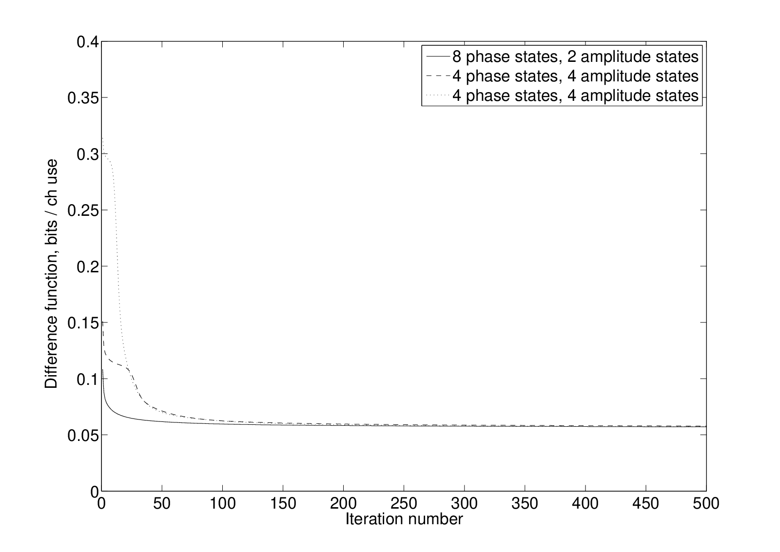
IX-E Upper Bound Tests

Fig. 12 shows $200$ iterations for the optimizing of the upper bound. The original fading channel has a normalized Doppler frequency shift of $f_{\mathrm{D}}T=0.1$ and the average SNR is $16$ dB. We have used the “natural initialization method” with $\hat{K}_{\theta}=8$ phase states $\hat{K}_{a}=2$ amplitude states. It is observed from this figure that if enough number of iterations are allowed, one is able to optimize the upper bound well below the CSI upper bound (the new upper bound is $0.8643$ bits / channel use, whereas the CSI upper bound is $0.9736$ bits / channel use.)

Furthermore, we observed that initializing the upper bound optimization algorithm by the “optimized difference function initialization method” may provide higher initial upper bounds that do not improve with further iterations. This may be due to the fact that this initialization method yields parameters where the upper bound has a local minimum, whereas the “natural initialization method” yields parameters at a non-stationary point of the upper bound, which can subsequently be improved iteratively. So for the upper bound, the “natural initialization method” with about $100$ to $200$ iterations is recommended.

IX-F Lower Bound Tests

Table III shows examples of obtained lower bounds based on a variety of initialization methods. Namely, the “natural initialization methods” and the “optimized difference function initialization method” are used with four and five, respectively, different settings of amplitude and phase states.

The original Gauss-Markov fading channel has a normalized Doppler frequency shift of $f_{\mathrm{D}}T=0.1$ and the average SNR is $0$ dB. The number of states in the AB-FSMC model is set to $16$ states. We used $\Gamma=\{1,1.5,2,2.5,\ldots,9.5,10,100\}$ in Algorithm 38 for choosing $\gamma$ at each iteration, where $\gamma=100$ has a stabilizing effect for $\hat{v}$ and does not let the lower bound decrease over iterations. It is clear from this table that initialization based on the “optimized difference function initialization method” can result in a higher information rate lower bound. For this initialization method we also observe that increasing the number of iterations from $50$ to $3000$ yields an improvement of only $0.0028$ bits / channel use, which is negligible for all practical purposes.

Finally, we would like to emphasize the importance of optimizing the lower bound from the mismatched decoding perspective. FSMC models have been proposed in the literature [31, 32, 33, 34, 35, 36] for channel estimation and decoding in time-varying, continuous-valued, and continuous state-space fading channels (see [29] for a review of FSMC-based decoding in fading channels). However, the fact that such decoding is mismatched to the physical fading channel often goes unnoticed. In particular, the choice of FSMC parameters (type of FSMC, number of amplitude and phase states, the FSMC state transition probabilities, and the FSMC output probabilities) are often chosen on an ad-hoc basis and mostly using the natural mapping of fading channel amplitude and phase into FSMC models. On the other hand, the results in this section showed that by optimizing the AB-FSMC parameters, we can achieve higher lower bounds on mismatched decoding rates and therefore achieve higher information rates in AB-FSMC-based decoding for fading channels.

Table III: The effect of different initialization methods on the lower bound. Better lower bounds are often obtained if the “optimized difference function initialization method” is used, which was observed to be a typical behavior of the lower bound across SNR.

Initialization Method	Best Lower Bound Found, bits / channel use
Natural, $\hat{K}_{\theta}=16$ , $\hat{K}_{a}=1$	$0.3357$
Natural, $\hat{K}_{\theta}=8$ , $\hat{K}_{a}=2$	$0.3501$
Natural, $\hat{K}_{\theta}=4$ , $\hat{K}_{a}=4$	$0.3345$
Natural, $\hat{K}_{\theta}=2$ , $\hat{K}_{a}=8$	$0.3056$
$50$ Iterations for Optimized Diff, $\hat{K}_{\theta}=16$ , $\hat{K}_{a}=1$	$0.3562$
$\mathbf{50}$ Iterations for Optimized Diff, $\mathbf{\hat{K}_{\theta}=8}$ , $\mathbf{\hat{K}_{a}=2}$	$\mathbf{0.3580^{*}}$
$\mathbf{3000}$ Iterations for Optimized Diff, $\mathbf{\hat{K}_{\theta}=8}$ , $\mathbf{\hat{K}_{a}=2}$	$\mathbf{0.3608^{**}}$
$50$ Iterations for Optimized Diff, $\hat{K}_{\theta}=4$ , $\hat{K}_{a}=4$	$0.3539$
$50$ Iterations for Optimized Diff, $\hat{K}_{\theta}=2$ , $\hat{K}_{a}=8$	$0.3529$

IX-G Optimized Bounds Versus SNR

Fig. 13 shows optimized upper and lower bounds for a practical range of SNRs and for the considered Gauss-Markov fading channel as in previous figures with a relatively fast fading rate of $f_{\mathrm{D}}T=0.1$ . We used $\Gamma=\{1,1.5,2,2.5,\ldots,9.5,10,100\}$ in Algorithm 38 for choosing $\gamma$ in the lower bound optimizations. The upper bound is considerably tighter than the CSI upper bound and together with the lower bound, can successfully bound the range of possible information rates. To the best of authors’ knowledge, no such good bounds have previously been shown in the literature.

X Conclusions

In this paper, we devised iterative algorithms for the minimization of an information rate upper bound and the maximization of an information rate lower bound for communication channels with memory. Moreover, we also discussed the minimization of the so-called difference function which represents the difference between the upper bound and a specialized version of the lower bound.

Our proposed optimization techniques are EM-type algorithms and optimize auxiliary FSMC models under the constraint that the (time-invariant) trellis is fixed. We applied the optimization techniques to original channels that are finite state (such as partial response channels) and non-finite state (such as fading channels). In both cases, we observed that the optimization techniques considerably tighten the bounds with a reasonable computational complexity. This is particularly important for finite-state channels with a large memory length ( $M\geq 10$ ), where the numerical computation of the information rate is complex, or for non-finite channels, where direct or numerical evaluation of the information rate is not possible. Using the proposed techniques, we improved the upper bound of the considered fading channel by as much as 0.11 bits / channel use below the CSI upper bound in binary signaling, which together with the optimized lower bound, successfully provided bounds for the fading channel information rates. Optimizing the lower bound is also significant from a mismatched decoding viewpoint for receivers that are equipped with the decoding metric for the auxiliary FSMC model, which is mismatched to the original communication channel.

Appendix A Proof of the Statement in Rem. 15

In this appendix we verify that $\sum_{{{\mathbf{\hat{s}}}},{{\mathbf{x}}}}\hat{v}({{\mathbf{\hat{s}}}},{{\mathbf{x}}},{{\mathbf{y}}})=1$ if $\sum_{\hat{s}_{\ell}}\hat{v}(\hat{s}_{\ell-1},x_{\ell},\hat{s}_{\ell},{{\mathbf{y}}}_{\ell-D_{1}}^{\ell+D_{2}})=1$ for all $\hat{s}_{\ell-1}$ , all $x_{\ell}$ , and all ${{\mathbf{y}}}_{\ell-D_{1}}^{\ell+D_{2}}$ . Indeed,

$\displaystyle\sum_{{{\mathbf{\hat{s}}}},{{\mathbf{x}}}}\hat{v}({{\mathbf{\hat{s}}}},{{\mathbf{x}}},{{\mathbf{y}}})$	$\displaystyle=\sum_{{{\mathbf{\hat{s}}}},{{\mathbf{x}}}}\prod_{\ell\in{{\mathcal{I}}}_{N}}Q\left(x_{\ell}\left\|x_{-N+1}^{\ell-1}\right.\right)\hat{v}\left(\hat{s}_{\ell-1},x_{\ell},\hat{s}_{\ell},{{\mathbf{y}}}_{\ell-D_{1}}^{\ell+D_{2}}\right)$	(88)
	$\displaystyle=\sum_{{{\mathbf{\hat{s}}}}_{-N+1}^{N-1},\,{{\mathbf{x}}}_{-N+1}^{N-1}}\prod_{\ell=-N+1}^{N-1}Q\left(x_{\ell}\left\|x_{-N+1}^{\ell-1}\right.\right)\hat{v}\left(\hat{s}_{\ell-1},x_{\ell},\hat{s}_{\ell},{{\mathbf{y}}}_{\ell-D_{1}}^{\ell+D_{2}}\right)$	(89)
	$\displaystyle\hskip 142.26378pt\cdot\ \underbrace{\sum_{x_{N}}Q\left(x_{N}\left\|x_{-N+1}^{N-1}\right.\right)\underbrace{\sum_{\hat{s}_{N}}\hat{v}\left(\hat{s}_{N-1},x_{N},\hat{s}_{N},{{\mathbf{y}}}_{N-D_{1}}^{N+D_{2}}\right)}_{=1}}_{=1}$	(90)
	$\displaystyle=\sum_{{{\mathbf{\hat{s}}}}_{-N+1}^{N-1},{{\mathbf{x}}}_{-N+1}^{N-1}}\prod_{\ell=-N+1}^{N-1}Q\left(x_{\ell}\left\|x_{-\ell+1}^{N-1}\right.\right)\hat{v}\left(\hat{s}_{\ell-1},x_{\ell},\hat{s}_{\ell},{{\mathbf{y}}}_{\ell-D_{1}}^{\ell+D_{2}}\right)$	(91)
	$\displaystyle=\cdots$	(92)
	$\displaystyle=1.$	(93)

Appendix B Proof of Lemma 20

For ease of reference, let us repeat here the relevant surrogate function:

\displaystyle\overline{\Psi}^{(N)}(\tilde{W},\hat{W})

\displaystyle\triangleq\overline{I}^{(N)}(\hat{W})+\frac{1}{2N}\sum_{{{\mathbf{y}}}}(QW)({{\mathbf{y}}})\,D_{{\mathbf{\hat{b}}}}\left(\tilde{P}({\mathbf{\hat{b}}}|{{\mathbf{y}}})\left\lVert\hat{P}({\mathbf{\hat{b}}}|{{\mathbf{y}}})\right.\right).

B-A Property 1

This follows from standard KL divergence properties.

B-B Property 2

Using the definition of $\overline{I}^{(N)}(\hat{W})$ in (27), we obtain

$\displaystyle\overline{\Psi}^{(N)}(\tilde{W},\hat{W})$	$\displaystyle=\frac{1}{2N}\sum\limits_{{{\mathbf{x}}},\,{{\mathbf{y}}}}Q({{\mathbf{x}}})W({{\mathbf{y}}}\|{{\mathbf{x}}})\log\left(W({{\mathbf{y}}}\|{{\mathbf{x}}})\right)$
	$\displaystyle\quad\ -\frac{1}{2N}\sum_{{{\mathbf{y}}}}(QW)({{\mathbf{y}}})\sum_{{\mathbf{\hat{b}}}}\tilde{P}({\mathbf{\hat{b}}}\|{{\mathbf{y}}})\log\left((Q\hat{W})({{\mathbf{y}}})\right)$
	$\displaystyle\quad\ +\frac{1}{2N}\sum_{{{\mathbf{y}}}}(QW)({{\mathbf{y}}})\sum_{{\mathbf{\hat{b}}}}\tilde{P}({\mathbf{\hat{b}}}\|{{\mathbf{y}}})\log\left(\tilde{P}({\mathbf{\hat{b}}}\|{{\mathbf{y}}})\right)$
	$\displaystyle\quad\ -\frac{1}{2N}\sum_{{{\mathbf{y}}}}(QW)({{\mathbf{y}}})\sum_{{\mathbf{\hat{b}}}}\tilde{P}({\mathbf{\hat{b}}}\|{{\mathbf{y}}})\log\left(\hat{P}({\mathbf{\hat{b}}}\|{{\mathbf{y}}})\right).$	(94)

We note that the first and third terms on the right-hand side are only functions of $Q$ , $W$ , $\tilde{W}$ , and are independent of $\hat{W}$ . By combining these two terms as $\overline{c}^{(N)}_{1}(\tilde{W})$ and by combining the second and fourth terms, we can write

\displaystyle\overline{\Psi}^{(N)}(\tilde{W},\hat{W})

\displaystyle=\overline{c}^{(N)}_{1}(\tilde{W})-\frac{1}{2N}\sum_{{{\mathbf{y}}}}(QW)({{\mathbf{y}}})\sum_{{\mathbf{\hat{b}}}}\tilde{P}({\mathbf{\hat{b}}}|{{\mathbf{y}}})\log\left(\hat{P}({\mathbf{\hat{b}}},{{\mathbf{y}}})\right).

Now using the AF-FSMC’s decomposition property (13) for $\hat{P}({\mathbf{\hat{b}}},{{\mathbf{y}}})=\hat{P}({{\mathbf{x}}},{{\mathbf{\hat{s}}}},{{\mathbf{y}}})$ , we can simplify the surrogate function further to

$\displaystyle\overline{\Psi}^{(N)}(\tilde{W},\hat{W})$	$\displaystyle=\overline{c}^{(N)}_{1}(\tilde{W})$
	$\displaystyle\quad\ -\frac{1}{2N}\sum_{{{\mathbf{y}}}}(QW)({{\mathbf{y}}})\sum_{{\mathbf{\hat{b}}}}\tilde{P}({\mathbf{\hat{b}}}\|{{\mathbf{y}}})\log\left(Q({{\mathbf{x}}})\right)$
	$\displaystyle\quad\ -\frac{1}{2N}\sum_{{{\mathbf{y}}}}(QW)({{\mathbf{y}}})\sum_{{\mathbf{\hat{b}}}}\tilde{P}({\mathbf{\hat{b}}}\|{{\mathbf{y}}})\sum_{\ell\in{{\mathcal{I}}}_{N}}\log\left(\hat{W}(\hat{s}_{\ell}\|\hat{s}_{\ell-1},x_{\ell})\right)$
	$\displaystyle\quad\ -\frac{1}{2N}\sum_{{{\mathbf{y}}}}(QW)({{\mathbf{y}}})\sum_{{\mathbf{\hat{b}}}}\tilde{P}({\mathbf{\hat{b}}}\|{{\mathbf{y}}})\sum_{\ell\in{{\mathcal{I}}}_{N}}\log\left(\hat{W}(y_{\ell}\|\hat{b}_{\ell})\right),$	(95)

where we notice that the second term on the right-hand side is independent of $\hat{W}$ . Therefore, by combining $\overline{c}^{(N)}_{1}(\tilde{W})$ and this term into $\overline{c}^{(N)}(\tilde{W})$ and after a few manipulations of the third and fourth terms, we obtain

\displaystyle\overline{\Psi}^{(N)}(\tilde{W},\hat{W})

\displaystyle=\overline{c}^{(N)}(\tilde{W})-\sum_{\hat{b}}\log\left(\hat{W}(\hat{s}|\hat{s}_{\mathrm{p}},x)\right)\tilde{T}^{(N)}_{1}(\hat{b})-\sum_{\hat{b}}\sum_{y}\log\left(\hat{W}(y|\hat{b})\right)\tilde{T}^{(N)}_{2}(\hat{b},y),

(96)

where $\tilde{T}^{(N)}_{1}(\hat{b})$ and $\tilde{T}^{(N)}_{2}(\hat{b},y)$ were defined in (40) and (41), respectively.

B-C Property 3

In order to prove convexity of $\overline{\Psi}^{(N)}(\tilde{W},\hat{W})$ w.r.t. $\bigl\{\hat{W}(\hat{s}|\hat{s}_{\mathrm{p}},x)\bigr\}\cup\bigl\{\hat{W}(y|\hat{b})\bigr\}$ , we need to show that the corresponding Hessian matrix is positive semi-definite. This can be done as follows. First, we use the expression in (96) for $\overline{\Psi}^{(N)}(\tilde{W},\hat{W})$ to obtain the following second-order partial derivatives:

		$\displaystyle\frac{\partial^{2}}{\partial{\hat{W}(\hat{s}\|\hat{s}_{\mathrm{p}},x)}^{2}}\overline{\Psi}^{(N)}=\frac{\tilde{T}^{(N)}_{1}(\hat{b})}{(\hat{W}(\hat{s}\|\hat{s}_{\mathrm{p}},x))^{2}},\quad\quad\frac{\partial^{2}}{\partial{\hat{W}(y\|\hat{b})}^{2}}\overline{\Psi}^{(N)}=\frac{\tilde{T}^{(N)}_{2}(\hat{b})}{(\hat{W}(y\|\hat{b}))^{2}},$		(97)
		$\displaystyle\frac{\partial^{2}}{\partial\hat{W}(\hat{s}\|\hat{s}_{\mathrm{p}},x)\partial\hat{W}(\hat{s}^{\prime}\|\hat{s}_{\mathrm{p}}^{\prime},x^{\prime})}\overline{\Psi}^{(N)}=0,\ \frac{\partial^{2}}{\partial\hat{W}(y\|\hat{b})\partial\hat{W}(y^{\prime}\|\hat{b}^{\prime})}\overline{\Psi}^{(N)}=0,\ \frac{\partial^{2}}{\partial\hat{W}(\hat{s}\|\hat{s}_{\mathrm{p}},x)\partial\hat{W}(y^{\prime}\|\hat{b}^{\prime})}\overline{\Psi}^{(N)}=0.$		(98)

Secondly, we note that $\tilde{T}^{(N)}_{1}(\hat{b})$ and $\tilde{T}^{(N)}_{2}(\hat{b},y)$ are non-negative, cf. (40) and (41). Thirdly, we combine these results and see that the Hessian matrix is diagonal with non-negative diagonal elements, i.e., the Hessian matrix is indeed positive semi-definite.

Let us remark that in the above computations of derivatives we did not impose the constraint that $\bigl\{\hat{W}(\hat{s}|\hat{s}_{\mathrm{p}},x)\bigr\}$ and $\bigl\{\hat{W}(y|\hat{b})\bigr\}$ lie in the corresponding probability simplices for every $(\hat{s}_{\mathrm{p}},x)$ and every $\hat{b}$ , respectively, and therefore we actually proved a stronger convexity result than really needed. Note that this approach of proving convexity worked well because the surrogate function is well-behaved also outside these probability simplices. This is in contrast to [10] where information rates where optimized as a function of source probabilities: for $N\to\infty$ , the information rate was not well defined outside the corresponding simplices and so it was important to take directional derivatives within the simplices. For more details we refer the reader to [10].

Appendix C Proof of Lemma 21

In this appendix, we minimize the surrogate function $\overline{\Psi}^{(N)}(\tilde{W},\hat{W})$ subject to the following constraints

	$\displaystyle\sum_{\hat{s}}\hat{W}(\hat{s}\|\hat{s}_{\mathrm{p}},x)$	$\displaystyle=1\quad(\text{for all $(\hat{s}_{\mathrm{p}},x)\in{\mathcal{\hat{S}}}\times{\mathcal{X}}$}),$		(99)
	$\displaystyle\sum_{y}\hat{W}(y\|\hat{b})$	$\displaystyle=1\quad(\text{for all $\hat{b}\in{\mathcal{\hat{B}}}$}).$		(100)

(For the moment we omit the non-negativity constraints; we will see at the end that they are automatically satisfied.) Clearly, the Lagrangian is

\displaystyle L

\displaystyle\triangleq\overline{\Psi}^{(N)}(\tilde{W},\hat{W})-\sum_{\hat{s}_{\mathrm{p}},x}\mu_{1}(\hat{s}_{\mathrm{p}},x)\left(\sum_{\hat{s}}\hat{W}(\hat{s}|\hat{s}_{\mathrm{p}},x)-1\right)-\sum_{\hat{b}}\mu_{2}(\hat{b})\left(\sum_{y}\hat{W}(y|\hat{b})-1\right),

(101)

where $\bigl\{\mu_{1}(\hat{s}_{\mathrm{p}},x)\bigr\}$ and $\bigl\{\mu_{2}(\hat{b})\bigr\}$ are Lagrange multipliers. Using the expression in (47) for $\overline{\Psi}^{(N)}(\tilde{W},\hat{W})$ and setting the derivative of $L$ w.r.t. $\hat{W}(\hat{s}|\hat{s}_{\mathrm{p}},x)$ equal to zero yields

\displaystyle\frac{\partial}{\partial\hat{W}(\hat{s}|\hat{s}_{\mathrm{p}},x)}L

\displaystyle=\frac{-1}{\hat{W}(\hat{s}|\hat{s}_{\mathrm{p}},x)}\tilde{T}^{(N)}_{1}(\hat{b})-\mu_{1}(\hat{s}_{\mathrm{p}},x)\overset{!}{=}0,

(102)

which results in

\displaystyle\hat{W}^{*}(\hat{s}|\hat{s}_{\mathrm{p}},x)

\displaystyle=\frac{\tilde{T}_{1}(\hat{b})}{-\mu_{1}(\hat{s}_{\mathrm{p}},x)}.

(103)

Therefore, the Lagrange multiplier $\mu_{1}(\hat{s}_{\mathrm{p}},x)$ is just a normalization constant so that $\sum_{\hat{s}}\hat{W}^{*}(\hat{s}|\hat{s}_{\mathrm{p}},x)=1$ . Since $\tilde{T}_{1}(\hat{b})$ is non-negative, cf. (40), non-negativity of the pmf $\hat{W}^{*}(\hat{s}|\hat{s}_{\mathrm{p}},x)$ is automatically satisfied. The optimum setting of $\hat{W}^{*}(y|\hat{b})$ is similarly found.

Appendix D Proof of Lemma 24

For ease of reference, let us repeat here the relevant surrogate function:

\displaystyle\Psi_{\Delta}^{(N)}(\tilde{W},\hat{W})

\displaystyle\triangleq\Delta^{(N)}(\hat{W})+\frac{1}{2N}\sum\limits_{{{\mathbf{x}}}}Q({{\mathbf{x}}})\sum\limits_{{{\mathbf{y}}}}W({{\mathbf{y}}}|{{\mathbf{x}}})\,D_{{\mathbf{\hat{b}}}}\left(\tilde{P}({\mathbf{\hat{b}}}|{{\mathbf{x}}},{{\mathbf{y}}})\left\lVert\hat{P}({\mathbf{\hat{b}}}|{{\mathbf{x}}},{{\mathbf{y}}})\right.\right).

(104)

D-A Property 1

This follows from standard KL divergence properties.

D-B Property 2

Using the definition (36) of difference function, the surrogate function in (104) is written as

$\displaystyle\Psi_{\Delta}^{(N)}(\tilde{W},\hat{W})$	$\displaystyle=\frac{1}{2N}\sum\limits_{{{\mathbf{x}}},\,{{\mathbf{y}}}}Q({{\mathbf{x}}})W({{\mathbf{y}}}\|{{\mathbf{x}}})\log\left(W({{\mathbf{y}}}\|{{\mathbf{x}}})\right)$
	$\displaystyle\quad\ -\frac{1}{2N}\sum\limits_{{{\mathbf{x}}},\,{{\mathbf{y}}}}Q({{\mathbf{x}}})W({{\mathbf{y}}}\|{{\mathbf{x}}})\sum\limits_{{\mathbf{\hat{b}}}}\tilde{P}({\mathbf{\hat{b}}}\|{{\mathbf{x}}},{{\mathbf{y}}})\log\left(\hat{W}({{\mathbf{y}}}\|{{\mathbf{x}}})\right)$
	$\displaystyle\quad\ +\frac{1}{2N}\sum\limits_{{{\mathbf{x}}},\,{{\mathbf{y}}}}Q({{\mathbf{x}}})W({{\mathbf{y}}}\|{{\mathbf{x}}})\sum\limits_{{\mathbf{\hat{b}}}}\tilde{P}({\mathbf{\hat{b}}}\|{{\mathbf{x}}},{{\mathbf{y}}})\log\left(\tilde{P}({\mathbf{\hat{b}}}\|{{\mathbf{x}}},{{\mathbf{y}}})\right)$
	$\displaystyle\quad\ -\frac{1}{2N}\sum\limits_{{{\mathbf{x}}},\,{{\mathbf{y}}}}Q({{\mathbf{x}}})W({{\mathbf{y}}}\|{{\mathbf{x}}})\sum\limits_{{\mathbf{\hat{b}}}}\tilde{P}({\mathbf{\hat{b}}}\|{{\mathbf{x}}},{{\mathbf{y}}})\log\left(\hat{P}({\mathbf{\hat{b}}}\|{{\mathbf{x}}},{{\mathbf{y}}})\right).$	(105)

The first and third terms on the right-hand side are only functions of $Q$ , $W$ , and $\tilde{W}$ and are independent of $\hat{W}$ . Therefore, by combining them as $c^{(N)}_{\Delta}(\tilde{W})$ , we can write

\displaystyle\Psi_{\Delta}^{(N)}(\tilde{W},\hat{W})

\displaystyle\triangleq c^{(N)}_{\Delta}(\tilde{W})-\frac{1}{2N}\sum\limits_{{{\mathbf{x}}},\,{{\mathbf{y}}}}Q({{\mathbf{x}}})W({{\mathbf{y}}}|{{\mathbf{x}}})\sum\limits_{{\mathbf{\hat{b}}}}\tilde{P}({\mathbf{\hat{b}}}|{{\mathbf{x}}},{{\mathbf{y}}})\log\left(\hat{P}({\mathbf{\hat{b}}},{{\mathbf{y}}}|{{\mathbf{x}}})\right).

Now using the AF-FSMC’s decomposition property (13) for $\hat{W}({\mathbf{\hat{b}}},{{\mathbf{y}}}|{{\mathbf{x}}})$ , we can simplify the surrogate function further to

$\displaystyle\Psi_{\Delta}^{(N)}(\tilde{W},\hat{W})$	$\displaystyle=c^{(N)}_{\Delta}(\tilde{W})$
	$\displaystyle\quad\ -\frac{1}{2N}\sum\limits_{{{\mathbf{x}}},\,{{\mathbf{y}}}}Q({{\mathbf{x}}})W({{\mathbf{y}}}\|{{\mathbf{x}}})\sum\limits_{{\mathbf{\hat{b}}}}\tilde{P}({\mathbf{\hat{b}}}\|{{\mathbf{x}}},{{\mathbf{y}}})\sum_{\ell\in{{\mathcal{I}}}_{N}}\log\left(\hat{W}(\hat{s}_{\ell}\|\hat{s}_{\ell-1},x_{\ell})\right)$	(106)
	$\displaystyle\quad\ -\frac{1}{2N}\sum\limits_{{{\mathbf{x}}},\,{{\mathbf{y}}}}Q({{\mathbf{x}}})W({{\mathbf{y}}}\|{{\mathbf{x}}})\sum\limits_{{\mathbf{\hat{b}}}}\tilde{P}({\mathbf{\hat{b}}}\|{{\mathbf{x}}},{{\mathbf{y}}})\sum_{\ell\in{{\mathcal{I}}}_{N}}\log\left(\hat{W}(y_{\ell}\|\hat{b}_{\ell})\right).$

After a few manipulations, we obtain

\displaystyle\Psi_{\Delta}^{(N)}(\tilde{W},\hat{W})

\displaystyle=c^{(N)}_{\Delta}(\tilde{W})-\sum_{\hat{b}}\log\left(\hat{W}(\hat{s}|\hat{s}_{\mathrm{p}},x)\right)\tilde{T}^{(N)}_{3}(\hat{b})-\sum_{\hat{b}}\sum_{y}\log\left(\hat{W}(y|\hat{b})\right)\tilde{T}^{(N)}_{4}(\hat{b},y).

(107)

where $\tilde{T}^{(N)}_{3}(\hat{b})$ and $\tilde{T}^{(N)}_{4}(\hat{b},y)$ were defined in (43) and (44), respectively.

D-C Property 3

Similarly to the proof of Property 3 of Lemma 20, the convexity of $\Psi_{\Delta}^{(N)}(\tilde{W},\hat{W})$ w.r.t. $W$ is established by looking at the corresponding Hessian matrix and by verifying that it is positive semi-definite. We leave the details to the reader.

Appendix E Proof of Lemma 29

For ease of reference, let us repeat here the relevant surrogate function:

\displaystyle\underline{\Psi}^{(N)}_{1}(\tilde{v},\hat{v})

\displaystyle\triangleq\underline{I}^{(N)}_{1}(\hat{v})-\frac{1}{2N}\sum\limits_{{{\mathbf{x}}},\,{{\mathbf{y}}}}Q({{\mathbf{x}}})W({{\mathbf{y}}}|{{\mathbf{x}}})D_{{{\mathbf{\hat{s}}}}}\left(\frac{\tilde{v}({{\mathbf{\hat{s}}}},{{\mathbf{x}}},{{\mathbf{y}}})}{\sum_{{{\mathbf{\hat{s}}}}^{\prime}}\tilde{v}({{\mathbf{\hat{s}}}}^{\prime},{{\mathbf{x}}},{{\mathbf{y}}})}\ \left\lVert\ \frac{\hat{v}({{\mathbf{\hat{s}}}},{{\mathbf{x}}},{{\mathbf{y}}})}{\sum_{{{\mathbf{\hat{s}}}}^{\prime}}\hat{v}({{\mathbf{\hat{s}}}}^{\prime},{{\mathbf{x}}},{{\mathbf{y}}})}\right.\right).

(108)

E-A Property 1

This follows from standard KL divergence properties.

E-B Property 2

Inserting the definition (60) of $\underline{I}^{(N)}_{1}(\hat{W})$ into (108), we obtain

\displaystyle\underline{\Psi}^{(N)}_{1}(\hat{v})

\displaystyle=\underline{c}^{(N)}_{1}(\tilde{v})+\frac{1}{2N}\sum\limits_{{{\mathbf{x}}},\,{{\mathbf{y}}}}Q({{\mathbf{x}}})W({{\mathbf{y}}}|{{\mathbf{x}}})\sum_{{{\mathbf{\hat{s}}}}}\frac{\tilde{v}({{\mathbf{\hat{s}}}},{{\mathbf{x}}},{{\mathbf{y}}})}{\sum_{{{\mathbf{\hat{s}}}}^{\prime}}\tilde{v}({{\mathbf{\hat{s}}}}^{\prime},{{\mathbf{x}}},{{\mathbf{y}}})}\log\big(\hat{v}({{\mathbf{\hat{s}}}},{{\mathbf{x}}},{{\mathbf{y}}})\big),

(109)

where $\underline{c}^{(N)}_{1}(\tilde{v})$ is independent of $\hat{v}$ . Applying the product decomposition (22) of $\hat{v}({{\mathbf{\hat{s}}}},{{\mathbf{x}}},{{\mathbf{y}}})$ , and the relationship (25), i.e.,

\displaystyle\frac{\tilde{v}({{\mathbf{\hat{s}}}},{{\mathbf{x}}},{{\mathbf{y}}})}{\sum_{{{\mathbf{\hat{s}}}}^{\prime}}\tilde{v}({{\mathbf{\hat{s}}}}^{\prime},{{\mathbf{x}}},{{\mathbf{y}}})}=\tilde{V}({{\mathbf{\hat{s}}}}|{{\mathbf{x}}},{{\mathbf{y}}}),

(110)

we get, after some simplifying steps,

\displaystyle\underline{\Psi}^{(N)}_{1}(\tilde{v},\hat{v})

\displaystyle=\underline{c}^{(N)}_{1}(\tilde{v})+\sum_{\hat{b}}\sum_{{{\mathbf{y}}^{\underline{D}}}}\log\left(\hat{v}(\hat{b},{{\mathbf{y}}^{\underline{D}}})\right)\tilde{T}^{(N)}_{4}(\hat{b},{{\mathbf{y}}^{\underline{D}}}).

(111)

E-C Property 3

Similarly to the proof of Property 3 of Lemma 20, the concavity of $\underline{\Psi}^{(N)}_{1}(\tilde{v},\hat{v})$ w.r.t. $\hat{v}$ is established by looking at the corresponding Hessian matrix and by verifying that it is negative semi-definite. We leave the details to the reader.

Appendix F Proof of Lemma 30

For ease of reference, let us repeat here the relevant part of the information rate lower bound and the corresponding surrogate function:

	$\displaystyle\underline{I}^{(N)}_{2}(\hat{v})$	$\displaystyle\triangleq-\frac{1}{2N}\sum\limits_{{{\mathbf{y}}}}(QW)({{\mathbf{y}}})\log\left(\sum_{{{\mathbf{\hat{s}}}}^{\prime},{{\mathbf{x}}}^{\prime}}\hat{v}({{\mathbf{\hat{s}}}}^{\prime},{{\mathbf{x}}}^{\prime},{{\mathbf{y}}})\right),$		(112)
	$\displaystyle\underline{\Psi}^{(N)}_{2}(\tilde{v},\hat{v})$	$\displaystyle\triangleq\underline{c}^{(N)}_{2}(\tilde{v})-\sum_{\hat{b}}\sum_{{{\mathbf{y}}^{\underline{D}}}}\frac{1}{\gamma}\left(\frac{\hat{v}(\hat{b},{{\mathbf{y}}^{\underline{D}}})}{\tilde{v}(\hat{b},{{\mathbf{y}}^{\underline{D}}})}\right)^{\gamma}\tilde{T}^{(N)}_{2}(\hat{b},{{\mathbf{y}}^{\underline{D}}}).$		(113)

F-A Property 1

This statement follows trivially from the definition of $\underline{c}_{2}(\tilde{v})$ .

F-B Property 2

On one hand, taking derivatives of $\underline{\Psi}^{(N)}_{2}(\tilde{v},\hat{v})$ w.r.t. $\hat{v}(\hat{b},{{\mathbf{y}}^{\underline{D}}})$ we obtain

\displaystyle\left.\frac{\partial}{\partial\hat{v}(\hat{b},{{\mathbf{y}}^{\underline{D}}})}\underline{\Psi}^{(N)}_{2}(\hat{v})\right|_{\hat{v}=\tilde{v}}

\displaystyle=\left.-\frac{\gamma}{\gamma}\cdot\frac{\hat{v}(\hat{b},{{\mathbf{y}}^{\underline{D}}})^{\gamma-1}}{\tilde{v}(\hat{b},{{\mathbf{y}}^{\underline{D}}})^{\gamma}}\cdot\tilde{T}^{(N)}_{2}(\hat{b},{{\mathbf{y}}^{\underline{D}}})\right|_{\hat{v}=\tilde{v}}=-\frac{1}{\tilde{v}(\hat{b},{{\mathbf{y}}^{\underline{D}}})}\cdot\tilde{T}^{(N)}_{2}(\hat{b},{{\mathbf{y}}^{\underline{D}}}).

(114)

On the other hand, $\underline{I}^{(N)}_{2}(\hat{v})$ can be expanded to the following expression

	$\displaystyle\underline{I}^{(N)}_{2}(\hat{v})$	$\displaystyle=\underline{c}^{(N)}_{2}(\tilde{v})-\frac{1}{2N}\sum\limits_{{{\mathbf{y}}}}(QW)({{\mathbf{y}}})\sum_{{{\mathbf{\hat{s}}}},{{\mathbf{x}}}}\frac{\tilde{v}({{\mathbf{\hat{s}}}},{{\mathbf{x}}},{{\mathbf{y}}})}{\sum_{{{\mathbf{\hat{s}}}}^{\prime},{{\mathbf{x}}}^{\prime}}\tilde{v}({{\mathbf{\hat{s}}}}^{\prime},{{\mathbf{x}}}^{\prime},{{\mathbf{y}}})}\log\left(\hat{v}({{\mathbf{\hat{s}}}},{{\mathbf{x}}},{{\mathbf{y}}})\right)$
		$\displaystyle\quad\ -\frac{1}{2N}\sum\limits_{{{\mathbf{y}}}}(QW)({{\mathbf{y}}})D_{{{\mathbf{\hat{s}}}},{{\mathbf{x}}}}\left(\frac{\tilde{v}({{\mathbf{\hat{s}}}},{{\mathbf{x}}},{{\mathbf{y}}})}{\sum_{{{\mathbf{\hat{s}}}}^{\prime},{{\mathbf{x}}}^{\prime}}\tilde{v}({{\mathbf{\hat{s}}}}^{\prime},{{\mathbf{x}}}^{\prime},{{\mathbf{y}}})}\ \left\lVert\ \frac{\hat{v}({{\mathbf{\hat{s}}}},{{\mathbf{x}}},{{\mathbf{y}}})}{\sum_{{{\mathbf{\hat{s}}}}^{\prime},{{\mathbf{x}}}^{\prime}}\hat{v}({{\mathbf{\hat{s}}}}^{\prime},{{\mathbf{x}}}^{\prime},{{\mathbf{y}}})}\right.\right),$		(115)

where $\underline{c}^{(N)}_{2}(\tilde{v})$ is independent of $\hat{v}$ . At first sight, expression (115) looks more complicated than expression (112), however, the relevant gradient of expression (115) is easier to find. Namely, the gradient of the first term with respect to $\hat{v}$ is the zero vector and so we do not have to worry about it. Similarly, the third term is a KL divergence and so the gradient with respect to $\hat{v}$ at $\hat{v}=\tilde{v}$ is also the zero vector. Therefore, we only need to have a close look at the second term. Applying the product decomposition (22) of $\hat{v}({{\mathbf{\hat{s}}}},{{\mathbf{x}}},{{\mathbf{y}}})$ , and using (21), i.e.,

\displaystyle\frac{\tilde{v}({{\mathbf{\hat{s}}}},{{\mathbf{x}}},{{\mathbf{y}}})}{\sum_{{{\mathbf{\hat{s}}}}^{\prime},{{\mathbf{x}}}^{\prime}}\tilde{v}({{\mathbf{\hat{s}}}}^{\prime},{{\mathbf{x}}}^{\prime},{{\mathbf{y}}})}

\displaystyle=\tilde{V}({{\mathbf{\hat{s}}}},{{\mathbf{x}}}|{{\mathbf{y}}}),

(116)

we get

	$\displaystyle\left.\frac{\partial}{\partial\hat{v}(\hat{b},{{\mathbf{y}}^{\underline{D}}})}\underline{I}^{(N)}_{2}(\hat{v})\right\|_{\hat{v}=\tilde{v}}$	$\displaystyle=\left.-\frac{\partial}{\partial\hat{v}(\hat{b},{{\mathbf{y}}^{\underline{D}}})}\sum_{\hat{b}^{\prime}}\sum_{({{\mathbf{y}}^{\underline{D}}})^{\prime}}\log\left(\hat{v}(\hat{b}^{\prime},({{\mathbf{y}}^{\underline{D}}})^{\prime})\right)\tilde{T}^{(N)}_{2}(\hat{b}^{\prime},({{\mathbf{y}}^{\underline{D}}})^{\prime})\right\|_{\hat{v}=\tilde{v}}$		(117)
		$\displaystyle=\left.-\frac{1}{\hat{v}(\hat{b},{{\mathbf{y}}^{\underline{D}}})}\cdot\tilde{T}^{(N)}_{2}(\hat{b},{{\mathbf{y}}^{\underline{D}}})\right\|_{\hat{v}=\tilde{v}}=-\frac{1}{\tilde{v}(\hat{b},{{\mathbf{y}}^{\underline{D}}})}\cdot\tilde{T}^{(N)}_{2}(\hat{b},{{\mathbf{y}}^{\underline{D}}}),$		(118)

which indeed agrees with the expression in (114).

F-C Property 3

Similarly to the proof of Property 3 of Lemma 20, the concavity of $\underline{\Psi}^{(N)}_{2}(\tilde{v},\hat{v})$ w.r.t. $\hat{v}$ is established by looking at the corresponding Hessian matrix and by verifying that it is negative semi-definite. We leave the details to the reader.

Acknowledgments

The work of Parastoo Sadeghi was partly supported under Australian Research Council’s Discovery Projects funding scheme (project number DP0773898). The authors acknowledge correspondence with Fredrik Rusek which motivated them to generate Fig. 6. They are also grateful to Henry Pfister for mentioning to them the papers by Mevel et al.

References

[1] J. G. Proakis, Digital Communications, 4th ed. New York: McGraw-Hill, 2000.
[2] E. Biglieri, J. Proakis, and S. Shamai, “Fading channels: Information-theoretic and communications aspects,” IEEE Trans. Inform. Theory, vol. 44, no. 6, pp. 2619–2692, Oct. 1998.
[3] D. Arnold, H.-A. Loeliger, P. O. Vontobel, A. Kavčić, and W. Zeng, “Simulation-based computation of information rates for channels with memory,” IEEE Trans. on Inform. Theory, vol. IT–52, no. 8, pp. 3498–3508, Aug. 2006.
[4] R. G. Gallager, Information Theory and Reliable Communication. New York: Wiley, 1968.
[5] D. Arnold and H.-A. Loeliger, “On the information rate of binary-input channels with memory,” in Proc. 2001 IEEE Int. Conf. on Communications, Helsinki, Finland, June 11–14 2001, pp. 2692–2695.
[6] V. Sharma and S. K. Singh, “Entropy and channel capacity in the regenerative setup with applications to Markov channels,” in Proc. IEEE Intern. Symp. on Inform. Theory, Washington, D.C., June 24–29 2001, p. 283.
[7] H. D. Pfister, J. B. Soriaga, and P. H. Siegel, “On the achievable information rates of finite-state ISI channels,” in Proc. IEEE GLOBECOM, San Antonio, TX, Nov. 2001, pp. 2992–2996.
[8] P. O. Vontobel and D. M. Arnold, “An upper bound on the capacity of channels with memory and constraint input,” in Proc. IEEE Inform. Theory Workshop, Cairns, Australia, Sept. 2-7 2001, pp. 147–149.
[9] S. Yang, A. Kavčić, and S. Tatikonda, “Feedback capacity of finite-state machine channels,” IEEE Trans. Inform. Theory, vol. 51, no. 3, pp. 799–810, Mar. 2005.
[10] P. O. Vontobel, A. Kavčić, D. Arnold, and H.-A. Loeliger, “A generalization of the Blahut-Arimoto algorithm to finite-state channels,” accepted for IEEE Trans. Inform. Theory, 2007.
[11] D. Arnold, H.-A. Loeliger, and P. O. Vontobel, “Computation of information rates from finite state/source channel models,” in Proc. 40th Allerton Conf. on Communications, Control, and Computing, Allerton House, Monticello, Illinois, USA, October 2–4 2002.
[12] A. Ganti, A. Lapidoth, and İ. E. Telatar, “Mismatched decoding revisited: general alphabets, channels with memory, and the wide-band limit,” IEEE Trans. on Inform. Theory, vol. IT–46, no. 7, pp. 2315–2328, 2000.
[13] L. R. Bahl, J. Cocke, F. Jelinek, and J. Raviv, “Optimal decoding of linear codes for minimizing symbol error rate,” IEEE Trans. Inform. Theory, vol. 20, no. 3, pp. 284–287, Mar. 1974.
[14] P. Sadeghi, P. O. Vontobel, and R. Shams, “Optimizing information rate bounds for channels with memory,” in Proc. IEEE Intern. Symp. on Inform. Theory, Nice, France, June 24–29 2007, pp. 171–175.
[15] A. Dempster, N. Laird, and D. Rubin, “Maximum likelihood from incomplete data via the EM algorithm,” Journal of the Royal Statistical Society, vol. 39, no. 1, pp. 1–38, 1977.
[16] W. H. Press, B. P. Flannery, S. A. Teukolsky, and W. T. Vetterling, Numerical Recipes in C, 2nd ed. Cambridge: Cambridge University Press, 1992.
[17] R. Shams, R. A. Kennedy, P. Sadeghi, and R. Hartley, “Gradient intensity-based registration of multi-modal images of the brain,” in Proc. IEEE International Conference on Computer Vision (ICCV), Rio de Janeiro, Brazil, Oct. 2007.
[18] E. N. Gilbert, “Capacity of a burst-noise channel,” Bell Syst. Tech. J., vol. 39, no. 9, pp. 1253–1265, Sept. 1960.
[19] E. O. Elliott, “Estimates of error rates for codes on burst-noise channels,” Bell Syst. Tech. J., vol. 42, no. 5, pp. 1977–1997, Sept. 1963.
[20] F. Le Gland and L. Mevel, “Exponential forgetting and geometric ergodicity in Hidden markov models,” Math. Control Signals Systems, vol. 13, pp. 63–93, 2000.
[21] T. M. Cover and J. A. Thomas, Elements of Information Theory, ser. Wiley Series in Telecommunications. New York: John Wiley & Sons Inc., 1991, a Wiley-Interscience Publication.
[22] A. Ganti, A. Lapidoth, and I. E. Telatar, “Mismatch decoding revisited: General alphabets, channels with memory, and the wide-band limit,” IEEE Trans. Inform. Theory, vol. 46, no. 7, pp. 2315–2328, Nov. 2000.
[23] L. E. Baum, “An inequality and associated maximization technique in statistical estimation for probabilistic functions of a Markov process,” Inequalities, vol. 3, pp. 1–8, 1972.
[24] C. F. J. Wu, “On the convergence properties of the EM algorithm,” Ann. Stat., vol. 11, no. 1, pp. 95–103, Mar. 1983.
[25] L. Mevel and L. Finesso, “Asymptotical statistics of misspecified hidden Markov models,” IEEE Trans. on Autom. Control, vol. AC–7, pp. 1123–1132, 2004.
[26] F. R. Kschischang, B. J. Frey, and H.-A. Loeliger, “Factor graphs and the sum-product algorithm,” IEEE Trans. on Inform. Theory, vol. IT–47, no. 2, pp. 498–519, Feb. 2001.
[27] R. H. Clarke, “A statistical theory of mobile-radio reception,” Bell Syst. Tech. J., vol. 47, no. 6, pp. 957–1000, 1968.
[28] P. Sadeghi and P. Rapajic, “On information rates of time-varying fading channels modeled as finite-state Markov channels,” to appear in IEEE Trans. Commun., 2008.
[29] P. Sadeghi, R. A. Kennedy, P. Rapajic, and R. Shams, “On finite-state Markov channel modeling of fading channels: principles and applications,” to appear in IEEE Signal Processing Mag., 2008.
[30] X. Deng and A. M. Haimovich, “Information rates of time varying Rayleigh fading channels,” in Proc. IEEE Int. Conf. Commun.(ICC), Paris, France, June 2004, pp. 573–577.
[31] A. J. Goldsmith and P. Varaiya, “Capacity, mutual information, and coding for finite-state Markov channels,” IEEE Trans. Inform. Theory, vol. 42, no. 3, pp. 868–886, May 1996.
[32] L. Li and A. J. Goldsmith, “Low-complexity maximum-likelihood detection of coded signals sent over finite-state Markov channels,” IEEE Trans. Commun., vol. 50, no. 4, pp. 524–531, Apr. 2002.
[33] C. Komninakis and R. D. Wesel, “Joint iterative channel estimation and decoding in flat correlated Rayleigh fading,” IEEE J. Select. Areas Commun., vol. 19, no. 9, pp. 1706–1717, Sept. 2001.
[34] T. Li, X. Jin, and O. M. Collins, “Successive decoding for finite state Markov modelled flat fading channels,” in Proc. IEEE Int. Symp. on Inform. Theory (ISIT), Seattle, WA, July 2006, pp. 11–15.
[35] H. Kong and E. Shwedyk, “Sequence detection and channel estimation over finite state Markov channels,” IEEE Trans. Veh. Technol., vol. 48, no. 3, pp. 833–839, May 1999.
[36] M. Riediger and E. Shwedyk, “Communication receivers based on Markov models of the fading channel,” IEE Proc. Commun., vol. 150, no. 4, pp. 275–279, Aug. 2003.

	$\displaystyle P_{{{\mathbf{S}}},{{\mathbf{Y}}}\|{{\mathbf{X}}},S_{-N}}({{\mathbf{s}}},{{\mathbf{y}}}\|{{\mathbf{x}}},s_{-N})$	$\displaystyle=\prod_{\ell\in{{\mathcal{I}}}_{N}}P_{S_{\ell},Y_{\ell}\|S_{\ell-1},X_{\ell}}(s_{\ell},y_{\ell}\|s_{\ell-1},x_{\ell})$		(2)
		$\displaystyle=\left(\prod_{\ell\in{{\mathcal{I}}}_{N}}P_{S_{\ell}\|S_{\ell-1},X_{\ell}}(s_{\ell}\|s_{\ell-1},x_{\ell})\right)\cdot\left(\prod_{\ell\in{{\mathcal{I}}}_{N}}P_{Y_{\ell}\|S_{\ell-1},X_{\ell},S_{\ell}}(y_{\ell}\|s_{\ell-1},x_{\ell},s_{\ell})\right),$		(3)

$\displaystyle W(s_{\ell}\|s_{\ell-1},x_{\ell})$	$\displaystyle\triangleq P_{S_{\ell}\|S_{\ell-1},X_{\ell}}(s_{\ell}\|s_{\ell-1},x_{\ell}),$	(4)
$\displaystyle W(y_{\ell}\|s_{\ell-1},x_{\ell},s_{\ell})$	$\displaystyle\triangleq P_{Y_{\ell}\|S_{\ell-1},X_{\ell},S_{\ell}}(y_{\ell}\|s_{\ell-1},x_{\ell},s_{\ell}),$	(5)
$\displaystyle W({{\mathbf{s}}},{{\mathbf{y}}}\|{{\mathbf{x}}},s_{-N})$	$\displaystyle\triangleq P_{{{\mathbf{S}}},{{\mathbf{Y}}}\|{{\mathbf{X}}},S_{-N}}({{\mathbf{s}}},{{\mathbf{y}}}\|{{\mathbf{x}}},s_{-N}),$	(6)
$\displaystyle W({{\mathbf{y}}}\|{{\mathbf{x}}},s_{-N})$	$\displaystyle\triangleq P_{{{\mathbf{Y}}}\|{{\mathbf{X}}},S_{-N}}({{\mathbf{y}}}\|{{\mathbf{x}}},s_{-N})=\sum_{{{\mathbf{s}}}}W({{\mathbf{s}}},{{\mathbf{y}}}\|{{\mathbf{x}}},s_{-N}).$	(7)

$\displaystyle\hat{P}({\mathbf{\hat{b}}},{{\mathbf{y}}}\|\hat{s}_{-N})$	$\displaystyle\triangleq\hat{P}({{\mathbf{x}}},{{\mathbf{\hat{s}}}},{{\mathbf{y}}}\|\hat{s}_{-N}),$	(15)
$\displaystyle\hat{P}({{\mathbf{x}}},{{\mathbf{y}}}\|\hat{s}_{-N})$	$\displaystyle\triangleq\sum_{{{\mathbf{\hat{s}}}}}\hat{P}({{\mathbf{x}}},{{\mathbf{\hat{s}}}},{{\mathbf{y}}}\|\hat{s}_{-N}),$	(16)
$\displaystyle\hat{P}({{\mathbf{y}}}\|\hat{s}_{-N})$	$\displaystyle\triangleq\sum_{{{\mathbf{x}}},\,{{\mathbf{\hat{s}}}}}\hat{P}({{\mathbf{x}}},{{\mathbf{\hat{s}}}},{{\mathbf{y}}}\|\hat{s}_{-N})=\sum_{{{\mathbf{x}}}}\hat{P}({{\mathbf{x}}},{{\mathbf{y}}}\|\hat{s}_{-N})=(Q\hat{W})({{\mathbf{y}}}\|\hat{s}_{-N}),$	(17)
$\displaystyle\hat{P}({\mathbf{\hat{b}}}\|{{\mathbf{y}}},\hat{s}_{-N})$	$\displaystyle\triangleq\frac{\hat{P}({\mathbf{\hat{b}}},{{\mathbf{y}}}\|\hat{s}_{-N})}{\hat{P}({{\mathbf{y}}}\|\hat{s}_{-N})},$	(18)
$\displaystyle\hat{P}({\mathbf{\hat{b}}}\|{{\mathbf{x}}},{{\mathbf{y}}},\hat{s}_{-N})$	$\displaystyle\triangleq\frac{\hat{P}({\mathbf{\hat{b}}},{{\mathbf{y}}}\|\hat{s}_{-N})}{\sum\limits_{{\mathbf{\hat{b}}}^{\prime}:\,\text{${\mathbf{\hat{b}}}^{\prime}$ is compatible with ${{\mathbf{x}}}$}}\hat{P}({\mathbf{\hat{b}}}^{\prime},{{\mathbf{y}}}\|\hat{s}_{-N})},$	(19)

	$\displaystyle\Delta^{(N)}(\hat{W})\triangleq\overline{I}(\hat{W})-\left.\underline{I}^{(N)}(\hat{V})\right\|_{\hat{V}({{\mathbf{x}}}\|{{\mathbf{y}}})=\frac{Q({{\mathbf{x}}})\hat{W}({{\mathbf{y}}}\|{{\mathbf{x}}})}{(Q\hat{W})({{\mathbf{y}}})}}$	$\displaystyle=\frac{1}{2N}\sum\limits_{{{\mathbf{x}}},\,{{\mathbf{y}}}}Q({{\mathbf{x}}})W({{\mathbf{y}}}\|{{\mathbf{x}}})\log\left(\frac{W({{\mathbf{y}}}\|{{\mathbf{x}}})}{\hat{W}({{\mathbf{y}}}\|{{\mathbf{x}}})}\right)$		(36)
		$\displaystyle=\frac{1}{2N}D_{{{\mathbf{x}}},{{\mathbf{y}}}}\left(Q({{\mathbf{x}}})W({{\mathbf{y}}}\|{{\mathbf{x}}})\,\left\lVert\,Q({{\mathbf{x}}})\hat{W}({{\mathbf{y}}}\|{{\mathbf{x}}})\right.\right),$		(37)

$\displaystyle H(Y_{0}\|{{\mathbf{Y}}}_{-N+1}^{-1},{{\mathbf{X}}}_{-N+1}^{0})$	$\displaystyle\geq H(Y_{0}\|{{\mathbf{Y}}}_{-N+1}^{-1},{{\mathbf{X}}}_{-N+1}^{0},G_{-D})$	(80)
	$\displaystyle=H(Y_{0}\|{{\mathbf{Y}}}_{-D+1}^{-1},{{\mathbf{X}}}_{-D+1}^{0},G_{-D})$	(81)
	$\displaystyle=H(Y_{D}\|{{\mathbf{Y}}}_{1}^{D-1},{{\mathbf{X}}}_{1}^{D},G_{0}).$	(82)

Abstract

I Introduction

I-A Motivation and Background

I-B Contributions and Organization

I-C Notations

II Source and Channel Models

Definition 1 (The Index Set)

II-A Source Model

Definition 2 (Source)

II-B Finite-State Machine Channels (FSMCs)

Definition 3 (Finite-State Machine Channels (FSMCs))

Example 4 (Partial Response Channel)

Example 5 (Gilbert-Elliott Channel)

Definition 6 (Data-Controllable FSMCs)

II-C General Channels with Memory

II-D Original Backward Channel Model

II-E Auxiliary Forward Finite-State Machine Channels

Definition 7 (AF-FSMCs)

Remark 8 (Induced pmfs)

II-F Auxiliary Backward Finite-State Machine Channels

Definition 9 (AB-FSMCs)

II-G Remarks

III Information Rates and Their Upper and Lower Bounds

Definition 10 (Information Rate)

Definition 11 (Information Rate Upper Bound Based on an AF-FSMC)

Definition 12 (Information Rate Lower Bound Based on an AB-FSMC)

Remark 13 (First Special Case of Information Rate Lower Bound)

Definition 14 (Difference Function)

Remark 15 (Second Special Case of Information Rate Lower Bound)

IV Optimization Methods and Definitions

IV-A Optimization Approach for the Information Rate Upper Bound

IV-B Optimization Approach for the Difference Function

IV-C Optimization Approach for the Information Rate Lower Bound

IV-D Some Key Quantities for Iterative Optimizations

Definition 16 (T~1(N)​(b^)\tilde{T}^{(N)}_{1}(\hat{b}), T~2(N)​(b^,y)\tilde{T}^{(N)}_{2}(\hat{b},y), and T~2(N)​(b^,𝐲D¯)\tilde{T}^{(N)}_{2}(\hat{b},{{\mathbf{y}}^{\underline{D}}}))

Algorithm 17 (Numerical/Stochastic Computation of T~1(N)​(b^)\tilde{T}^{(N)}_{1}(\hat{b}), T~2(N)​(b^,y)\tilde{T}^{(N)}_{2}(\hat{b},y), and T~2(N)​(b^,𝐲D¯)\tilde{T}^{(N)}_{2}(\hat{b},{{\mathbf{y}}^{\underline{D}}}))

Definition 18 (T~3(N)​(b^)\tilde{T}^{(N)}_{3}(\hat{b}), T~4(N)​(b^,y)\tilde{T}^{(N)}_{4}(\hat{b},y), and T~4(N)​(b^,𝐲D¯)\tilde{T}^{(N)}_{4}(\hat{b},{{\mathbf{y}}^{\underline{D}}}))

Algorithm 19 (Numerical/Stochastic Computation of T~3(N)​(b^)\tilde{T}^{(N)}_{3}(\hat{b}), T~4(N)​(b^,y)\tilde{T}^{(N)}_{4}(\hat{b},y), and T~4(N)​(b^,𝐲D¯)\tilde{T}^{(N)}_{4}(\hat{b},{{\mathbf{y}}^{\underline{D}}}))

V Optimizing the Information Rate Upper Bound

Lemma 20 (Important Properties of Ψ¯\overline{\Psi})

Lemma 21 (Minimizing the Surrogate Function Ψ¯\overline{\Psi})

Algorithm 22 (Iterative Optimization of the Information Rate Upper Bound)

Lemma 23 (Convergence Properties of the Iterative Optimization)

VI Optimizing the Difference Function

Lemma 24 (Important Properties of ΨΔ\Psi_{\Delta})

Lemma 25 (Minimizing the Surrogate Function ΨΔ\Psi_{\Delta})

Remark 26 (Simplification for Data-Controllable AF-FSMCs)

Algorithm 27 (Iterative Optimization of the Difference Function)

Lemma 28 (Convergence Properties of the Iterative Optimization)

VII Optimizing the Information Rate Lower Bound

Lemma 29 (Important Properties of Ψ¯1\underline{\Psi}_{1})

Lemma 30 (Important Properties of Ψ¯2\underline{\Psi}_{2})

Lemma 31 (Important Properties of Ψ¯\underline{\Psi})

Lemma 32 (Maximizing the Surrogate Function Ψ¯\underline{\Psi})

Algorithm 33 (Iterative Optimization of the Information Rate Lower Bound)

Remark 34 (Normalization)

Remark 35 (Convergence)

Remark 36 (Simplification for Data-Controllable Auxiliary FSMCs)

Remark 37 (Optimization of the Alternative Information Rate Lower Bound)

VIII Numerical Results for Partial Response Channels

VIII-A Source, Channel, and Auxiliary Channel Models

VIII-B Initialization Methods

VIII-C Soblex Optimization Algorithm

VIII-D Reduction in the Computational Complexity

VIII-E Original Partial Response Channel with Memory Length M=2M=2

VIII-E1 Upper Bound Tests

VIII-E2 Lower Bound Tests

Algorithm 38 (An algorithm for choosing γ\gamma in (66))

VIII-F Original Partial Response Channel with Memory Length M=3M=3

VIII-F1 Upper Bound Tests

VIII-F2 Lower Bound Tests

IX Numerical Results for Fading Channels

IX-A Source, Channel, and Auxiliary Channel Models

IX-B Initialization Methods

IX-C A Lower Bound on HH

IX-D Optimizing the Difference Function

IX-E Upper Bound Tests

IX-F Lower Bound Tests

IX-G Optimized Bounds Versus SNR

X Conclusions

Definition 16 ( $\tilde{T}^{(N)}_{1}(\hat{b})$ , $\tilde{T}^{(N)}_{2}(\hat{b},y)$ , and $\tilde{T}^{(N)}_{2}(\hat{b},{{\mathbf{y}}^{\underline{D}}})$ )

Algorithm 17 (Numerical/Stochastic Computation of $\tilde{T}^{(N)}_{1}(\hat{b})$ , $\tilde{T}^{(N)}_{2}(\hat{b},y)$ , and $\tilde{T}^{(N)}_{2}(\hat{b},{{\mathbf{y}}^{\underline{D}}})$ )

Definition 18 ( $\tilde{T}^{(N)}_{3}(\hat{b})$ , $\tilde{T}^{(N)}_{4}(\hat{b},y)$ , and $\tilde{T}^{(N)}_{4}(\hat{b},{{\mathbf{y}}^{\underline{D}}})$ )

Algorithm 19 (Numerical/Stochastic Computation of $\tilde{T}^{(N)}_{3}(\hat{b})$ , $\tilde{T}^{(N)}_{4}(\hat{b},y)$ , and $\tilde{T}^{(N)}_{4}(\hat{b},{{\mathbf{y}}^{\underline{D}}})$ )

Lemma 20 (Important Properties of $\overline{\Psi}$ )

Lemma 21 (Minimizing the Surrogate Function $\overline{\Psi}$ )

Lemma 24 (Important Properties of $\Psi_{\Delta}$ )

Lemma 25 (Minimizing the Surrogate Function $\Psi_{\Delta}$ )

Lemma 29 (Important Properties of $\underline{\Psi}_{1}$ )

Lemma 30 (Important Properties of $\underline{\Psi}_{2}$ )

Lemma 31 (Important Properties of $\underline{\Psi}$ )

Lemma 32 (Maximizing the Surrogate Function $\underline{\Psi}$ )

VIII-E Original Partial Response Channel with Memory Length $M=2$

Algorithm 38 (An algorithm for choosing $\gamma$ in (66))

VIII-F Original Partial Response Channel with Memory Length $M=3$

IX-C A Lower Bound on $H$