Determining the motion of the solar system relative to the cosmic microwave background using type Ia supernovae

The cosmic microwave background (CMB) has a 3.4 mK dipole anisotropy (Hinshaw et al. 2007) which can naturally be explained as being due to the motion of the solar system with respect to the CMB rest frame (Lynden-Bell et al. 1989; Strauss et al. 1992; Erdogdu et al. 2006; Loeb & Narayan 2007). An interesting consistency check of this is to evaluate the solar system motion from peculiar velocity surveys (see for example Dale & Giovanelli 2000).

SNe luminosity measurements provide an accurate probe of peculiar velocities. Using observed correlations between SNe light curves, we can estimate the SNe absolute magnitudes and thus obtain accurate distance estimates to the SNe. Combined with spectroscopic measurements of the host galaxies’ redshifts, this can be used to estimate the peculiar velocity of each SNe’s host galaxy. The motion of the solar system will then show up as a dipole anisotropy in the SNe derived peculiar velocities. It is interesting to compare the estimates of the solar system motion from the SNe with those derived from the CMB. If they turn out to be inconsistent then it may be an indication that there is a significantly large intrinsic temperature dipole on the CMB surface of last scattering (Turner 1991; Langlois & Piran 1996), which could be caused by a double inflation model (Langlois 1996) for example.

A number of studies have made this comparison (Riess et al. 1995; Bonvin et al. 2006; Jha et al. 2007), and a simplifying assumption used in these studies was that the peculiar velocities of the individual SNe were uncorrelated with each other. However, as the peculiar velocities are caused by variations in the density field, neighbouring SNe will have correlated peculiar velocities (Wang et al. 1998; Sugiura et al. 1999; Hui & Greene 2006; Bonvin et al. 2006; Gordon et al. 2007). These correlations will increase the error bars on our peculiar velocity estimate as each new SNe measurement does not represent a completely independent realization of the velocity field.

In this article we include the correlations of the peculiar velocities when estimating the motion of the solar system with respect to the cosmic rest frame. In Sec. 2 we give a simple example of the underestimation of the uncertainty that occurs when correlations between observations are not taken into account. In Sec. 3 we outline the formalism we use for the SNe correlations, and in Sec. 4 we apply the method to SALT calibrated SNe data. In Sec. 5 we look at the implications for future surveys. A summary and discussion of the results is given in Sec. 6.

In order to illustrate the effect of correlated errors we consider a simple example (also discussed in Eq. 5 and its below paragraph of Cooray & Caldwell 2006) where we analyse $N$ data points ($x_{i}$) drawn from a multivariate Gaussian likelihood

$${\cal L}\propto|{\bf\sf C}|^{-1/2}\exp(-({\bf x}-\mn@boldsymbol{\mu})^{\rm T}{\bf\sf C}^{-1}({\bf x}-\mn@boldsymbol{\mu})/2).$$

(1)

The vector ${\bf x}$ is made up of the data points ($x_{i}$) and each element of the vector $\mn@boldsymbol{\mu}$ is equal to a constant, $\mu$. The covariance matrix (${\bf\sf C}$) has diagonal terms which are $\sigma^{2}$ and the off-diagonal terms which are $\rho\sigma^{2}$. That is each data point has correlation $\rho$ with the other data points. Suppose that one attempts to estimate the value of $\mu$ and $\sigma^{2}$ from the data and ignores correlations (i.e. assume $\rho$ to be zero). The maximum likelihood estimators of the mean and variance are then respectively given by

$$m={1\over N}\sum x_{i},\quad\quad s^{2}={1\over N}\sum_{i=1}^{N}(x_{i}-m)^{2}.$$

(2)

As the likelihood is a multivariate Gaussian distribution

$$\left<x_{i}\right>=\mu\quad\mbox{and}\quad\left<(x_{i}-\mu)(x_{j}-\mu)\right>={\sf C}_{i,j}$$

(3)

where angular brackets denote the expectation value. Evaluating Eq. (2) using Eq. (3) gives

$$\left<m\right>=\mu,\quad\quad\left<s^{2}\right>\approx(1-\rho)\sigma^{2}$$

(4)

in the large N limit, where the approximation approaches equality for large $N$. As can be seen from the above equation, $m$ is an unbiased estimator of the true mean, even when there are correlations in the data. However, as can also be seen, $s^{2}$ is biased by a factor of $(1-\rho)$.

If there where no correlations, the error on $\mu$ can be estimated by

$$\delta\mu=\frac{s}{\sqrt{N}}\,.$$

(5)

If there are correlations present then it follows from Eq. (4) that this estimator will give

$$\delta\mu=\sigma\sqrt{\frac{1-\rho}{N}}.$$

(6)

Now we find the correct value of $\delta\mu$ to see the effects of ignoring correlations. For large $N$, the expectation of the one sigma error on $\mu$ can be approximated

$$\delta\mu\approx\sqrt{({\sf F}^{-1})_{\mu,\mu}}$$

(7)

where $({\sf F}^{-1})_{\mu,\mu}$ is the $(\mu,\mu)$ component of the inverse of the Fisher matrix. For a multivariate Gaussian likelihood the Fisher matrix is given by (see for example Tegmark et al. 1997)

	$\displaystyle{\bf\sf F}_{\alpha,\beta}$	$\displaystyle\equiv$	$\displaystyle-\left<\frac{\partial^{2}\ln{\mathcal{L}}}{\partial p_{\alpha}\partial p_{\beta}}\right>$		(8)
		$\displaystyle=$	$\displaystyle\mn@boldsymbol{\mu}_{,\alpha}{\bf\sf C}^{-1}\mn@boldsymbol{\mu}{{}^{\rm T}}_{,\beta}+\frac{1}{2}{\rm Tr}\left({\bf\sf C}{{}^{-1}}{\bf\sf C}_{,\alpha}{\bf\sf C}{{}^{-1}}{\bf\sf C}_{,\beta}\right)$		(9)

where $\alpha$ and $\beta$ run over the different model parameters which are being estimated ($\mu$ and $\sigma$, with $\rho$ assumed known, in the current example). Eq. (9) gives the true error on the value of $\mu$, and in our example this is

$$\delta\mu_{{\rm corr}}=\sigma\sqrt{\frac{1+(N-1)\rho}{N}}.$$

(10)

Comparing Eqs. (6) and (10) we see that if the data are correlated ($\rho>0$) but correlations are neglected then one would underestimate the uncertainty on $\mu$. One would overestimate the error if the data is anti-correlated, although we note that this case is restricted as for the covariance matrix to be positive definite, $\rho>-(N-1)^{-1}$.

As was shown in a earlier studies (Hui & Greene 2006; Neill et al. 2007; Gordon et al. 2007), an analogous underestimation of the error happens if the correlations in low redshift SNe are not accounted for when using them in a sample to estimate the dark energy equation of state, $w$. In this article we show that there is also an underestimation in error on the motion of our solar system when the correlations in the SNe are not accounted for.

The luminosity distance, $d_{L}$, to a SN at redshift $z$, is defined such that

$${\mathcal{F}}=\frac{\mathcal{L}}{4\pi d_{L}^{2}}$$

where $\mathcal{F}$ is the observed flux and $\mathcal{L}$ is the SN’s intrinsic luminosity. Astronomers use magnitudes, which are related to the luminosity distance (in megaparsec) by

$$m-M=5\log_{10}d^{obs}_{L}+25,$$

(11)

where $m$ and $M$ are the apparent and absolute magnitudes respectively. In the context of SNe, $M$ is a “nuisance parameter” which is completely degenerate with $\log(H_{0})$ and is marginalised over. For a Friedmann-Robertson-Walker Universe the predicted luminosity distance is given by

$$d_{L}(z)=(1+z)\int_{0}^{z}\frac{{{\rm d}}z^{\prime}}{H(z^{\prime})}$$

(12)

(taking $c=1$), where $H$ is the Hubble parameter. In the limit of low redshift this reduces to $d_{L}\approx z/H_{0}$.

Given very stringent limits on the curvature of the universe, we can safely work within the assumption of a flatness as the allowed curvature would not play any role at the scales of interest. In this case, the effect of a peculiar velocity (PV) leads to a perturbation in the luminosity distance ($\delta d_{L}$) given by  (Sasaki 1987; Sugiura et al. 1999; Pyne & Birkinshaw 2004; Bonvin et al. 2006; Hui & Greene 2006)

$$\frac{\delta d_{L}}{d_{L}}=\hat{\bf r}\cdot\left({\bf v}-\frac{(1+z)^{2}}{H(z)\>d_{L}}[{\bf v}-{\bf v}_{O}]\right)$$

(13)

where ${\bf r}$ is the position of the SN, and ${\bf v}_{O}$ and ${\bf v}$ are the peculiar velocites of the observer and SN repectively. In the limit of low redshift, $\delta d_{L}\approx\hat{\bf r}\cdot[{\bf v}_{O}-{\bf v}]/H_{0}$. This demonstrates how a SNe survey that measures $m$ and $z$ can estimate the projected PV field. We now relate this to the cosmology.

The projected velocity correlation function, $\xi({\bf r},{\bf r^{\prime}})\equiv\left<({\bf v}({\bf r})\cdot\hat{\bf r})({\bf v}({\bf r^{\prime}})\cdot\hat{\bf r}^{\prime})\right>$, must be rotationally invariant, and therefore it can be decomposed into a parallel and perpendicular components (Gorski 1988; Groth et al. 1989; Dodelson 2003) :

$$\xi({\bf r},{\bf r^{\prime}})=\sin\theta\sin\theta^{\prime}\xi_{\perp}(\Delta r,z,z^{\prime})+\cos\theta\cos\theta^{\prime}\xi_{\parallel}(\Delta r,z,z^{\prime})$$

(14)

where $\Delta{\bf r}\equiv{\bf r}-{\bf r}^{\prime}$, $\Delta r=|\Delta{\bf r}|$, $\cos\theta\equiv\hat{\bf r}\cdot\Delta\hat{\bf r}$, and $\cos\theta^{\prime}\equiv\hat{\bf r}^{\prime}\cdot\Delta\hat{\bf r}$. In linear theory, these are given by (Gorski 1988; Groth et al. 1989; Dodelson 2003):

$$\xi_{\parallel,\perp}=D^{\prime}(z)\>D^{\prime}(z^{\prime})\>\int_{0}^{\infty}\frac{\rm dk}{2\pi^{2}}P(k)K_{\parallel,\perp}(kr)$$

(15)

where for an arbitrary variable $x$, $K_{\parallel}(x)\equiv j_{0}(x)-\frac{2j_{1}(x)}{x}$, $K_{\perp}(x)\equiv j_{1}(x)/x$. $D(z)$ is the growth function, and derivatives are with respect to conformal time. $P(k)$ is the matter power spectrum which can be evaluated either numerically (e.g. CAMB Lewis et al. 2000) or using analytical approximations (Eisenstein & Hu 1998).

The above estimate of $\xi({\bf r},{\bf r}^{\prime})$ is based on linear theory. On scales smaller than about 10$h^{-1}$Mpc, nonlinear contributions dominate. These are usually modeled as an uncorrelated term which is independent of redshift, often set to $\sigma_{v}\sim 300$ km/s. Comparison with N-body simulations (Silberman et al. 2001) indicate that this is an effective way of accounting for the non-linearities. Other random errors that are usually considered are those from the lightcurve fitting ($m_{\rm err}$), and intrinsic magnitude scatter ($\sigma_{m}$) . It is just these three errors that are usually included in the analysis of SNe.

The residual deviations of luminosity distance from the homogeneous expansion can be packed into a data vector

$$\left(\frac{\delta d_{L}}{d_{L}}\right)_{i}=\frac{d_{L}^{obs}(i)-d_{L}(z(i))}{d_{L}(z(i))},$$

(16)

whose covariance matrix (from the correlated PVs) is given by

$${\sf C}_{v}(i,j)=\left(1-\frac{(1+z)^{2}}{H\>d_{L}}\right)_{i}\left(1-\frac{(1+z)^{2}}{H\>d_{L}}\right)_{j}\xi({\bf r_{\bf i}},{\bf r_{\bf j}}),$$

(17)

while the standard uncorrelated random errors are given by

$$\sigma(i)^{2}=\left({\ln(10)\over 5}\right)^{2}(\sigma_{m}^{2}+m_{\rm err}(i)^{2})+\left(1-\frac{(1+z)^{2}}{H\>d_{L}}\right)_{i}^{2}\sigma_{v}^{2}.$$

(18)

Some example plots of ${\sf C}_{v}$ were given in Gordon et al. 2007. The likelihood is then

$${\cal L}=(2\pi)^{-N/2}|{\bf\sf\Sigma}|^{-1/2}\exp\left({-{1\over 2}{\mathbf{\Delta}}^{T}{\bf\sf\Sigma}^{-1}{\mathbf{\Delta}}}\right)$$

(19)

where

$${\sf\Sigma}(i,j)={\sf C}_{v}(i,j)+\sigma(i)^{2}{\sf\delta}_{ij}$$

(20)

and

$$\Delta_{i}=\left(\frac{\delta d_{L}}{d_{L}}\right)_{i}-\left(\frac{(1+z)^{2}}{H(z)\>d_{L}}\right)_{i}\hat{\bf r}_{i}\cdot{\bf v}_{O}.$$

(21)

We now proceed to find constraints on the observer velocity ${\bf v}_{O}$. We assume a standard $\Lambda$CDM cosmology and impose Big Bang Nucleosynthesis (BBN) prior $\Omega_{b}h^{2}\sim{\mathcal{N}}(0.0214,0.002)$ (Kirkman et al. 2003), and a Hubble Space Telescope (HST) prior $h\sim{\cal N}(0.72,0.08)$ (Freedman et al. 2001). These two priors remove models that are wildly at odds with standard cosmological probes, but do not unduly bias results towards standard cosmology. The likelihood has almost negligible dependence on $n_{s}$, and to keep it in a range consistent with CMB and large scale structure estimates we give it a uniform prior $n\in[-0.9,1.1]$.

We parameterize the solar system peculiar velocity as a magnitude ($v_{O}$) and direction in galactic coordinates $(l,b)$. The prior on $(l,b)$ was assumed to be uniform on the sphere, i.e flat on $l$ and $\cos(b)$. The prior on $v_{O}$ was set to be uniform.

We use a SALT (Guy et al. 2005) calibrated low redshift SNe data set¹¹ 1 Obtained from http://qold.astro.utoronto.ca/conley/bubble/ with heliocentric redshifts in the range $cz\in[2278,37163]$km/s, ($z\in[0.0076,0.124]$). A histogram of the 61 redshifts is shown in Fig. 1 and the sky positions of the data are shown in Fig. 2.

We also used the higher redshift 71 SNe from the SNLS data set.²² 2 Obtained from http://snls.in2p3.fr/conf/papers/cosmo1/

The SALT calibration involves the additional parameters ($\alpha$, $\beta$), which account for the shape/luminosity and colour/luminosity relations of SNe. These and the other parameters $(\Omega_{m},\sigma_{8},\sigma_{v},\sigma_{m},M)$ are all given broad uniform priors. We use the standard Markov Chain Monte Carlo (MCMC) method to generate samples from the posterior distribution of the parameters (Lewis & Bridle 2002). Convergence was checked using multiple chains with different starting positions, and also the $R-1$ statistic  (Gelman & Rubin 1992). We also checked that the estimated posterior distributions reduced to the prior distributions when no data was used.The analysis was checked with two completely independent codes and MCMC chains.

Additionally, we looked at the combination of the SNe observations with the WMAP data of the CMB (Spergel et al. 2006) (with the usual CMB priors in this case). We stress that we do not use the WMAP dipole information, but rather just the $\ell>1$ information, which when combined with the SNe has the effect of constraining matter density and the amplitude of matter fluctuations.

In Fig. 3 we plot the marginalized probability contours for $v_{O}$ and $\sigma_{8}$, where we see that higher values of $\sigma_{8}$ have broader contours on $v_{O}$. This is because a larger $\sigma_{8}$ implies more correlations between the SNe peculiar velocities and so less of a reduction in the errors due to averaging effects. The contours for when WMAP is included are also plotted.

In Fig. 4 a marginalized probability distribution is plotted for $v_{O}$, and we see that the uncertainty on $v_{O}$ increases dramatically when the correlations are accounted for. It can also be seen that adding WMAP data has a negligible effect. As seen from Fig. 3, this arises because the WMAP data constrains $\sigma_{8}\approx 0.8$, which happens to lie on an approximately average value for the $v_{O}$ uncertainty. In Fig. 5 the one sigma confidence intervals are plotted for the direction of the solar system motion. As can be seen, not accounting for the correlations underestimates the uncertainty by about a factor of 2.

Also, Figs. 4 and 5 shows that the SNe data are consistent with the CMB dipole estimate of $(v_{O},l,b)=(369\pm 3{\rm km/s},263.86\pm 0.04^{\circ},48.24\pm 0.10^{\circ})$ (Hinshaw et al. 2007). In Table 1 the mean and uncertainties of the solar system peculiar velocity are given. We find that when the correlations are not included, the estimate of $v_{O}$ is about 3.5 standard deviations from zero. While if the correlations are accounted for then $v_{O}$ is only about 2.5 standard deviations from zero. One can convert the number of standard deviations of the detection into upper bounds on the Bayesian odds ratio (Gordon & Trotta 2007). Without correlations the odds, from SNe data, of $v_{O}$ being non-zero appear to be at best 119:1. While if the correlations are accounted for then the odds are at best only 7:1. In Table 1 we also give an estimate for the local group motion which was obtained by subtracting the solar system velocity relative to the local group (Yahil et al. 1977).

In this section we forecast constraints on the motion of the solar system from GAIA (the “super-Hipparcos” satellite) and LSST. For GAIA, based on the simulations by Belokurov & Evans 2003, we generate a sample of 6,317 SNe distributed over the full sky with $z<0.14$. For LSST we generate 30,000 SNe distributed over the full sky with $z<0.3$ (Wang et al. 2005). We weighted the distribution of SNe by $\cos(b)z^{2}$ to account for the volume in spherical coordinates, that is we keep the density constant with $z$. As our fiducial model we took $\{v_{O},l,b,\Omega_{m},\Omega_{b},h,n_{s},w,\sigma_{8},\sigma_{v},\sigma_{m},m_{err}\}=\{369,264^{\circ},48^{\circ},0.3,0.041,0.72,0.96,-1,0.85,300,0.1,0.1\}$. We do not include the SALT calibration parameters $(\alpha,\beta)$ in the forecast, but we have checked using forecasts for the data sets used in Sec. 3 that this does not have a significant effect. In order to use the Fisher matrix (see Eq. (9)), we consider the function

$$d=d_{L}^{\rm obs}\>10^{M_{0}/5}$$

(22)

where $d_{L}^{\rm obs}$ is given by Eq.(11). The expectation value vector has each element given by

$$\left<d\right>=10^{M_{0}/5}\left(d_{L}^{\rm th}+\hat{{\bf r}}\cdot{\bf v}_{O}\>\frac{(1+z)^{2}}{H(z)}\right),$$

(23)

with $d_{L}^{\rm th}$ given by Eq.(12). The covariance matrix $({\bf\sf C})$ is as before, Eq.(20), but with the extra factor $\left(10^{M_{0}/5}\right)^{2}d_{L}(i)d_{L}(j)$. Note the reason for the slightly different function of the data compared to Eq. (21) is so that the data vector does not depend on any of the parameters.

In Table 2 we present our main forecast results.

As can be seen there is a dramatic improvement in the constraints compared to current data. Also, unlike current data, taking into account the correlations does not have a large effect. This is because most of the constraining power for GAIA and LSST comes from higher redshifts, where the peculiar velocity errors are negligible compared to the other types of error. This can be understood as follows. From Eq. 17 we see that the error induced by peculiar coherent velocity flows drops as $1/z$, and thus for high enough redshift ($z>0.015$ for a typical experiment) they become unimportant compared to the redshift independent measurement errors in Eq. (18). In this limit the weakening of the dipole signal, that drops as $1/z$ in Eq.(21), is exactly compensated by the number of supernova in a redshift slice, which increases as $z^{2}$, for a volume-weighted survey. The signal to noise is therefore low and increasing at low redshift, tailing off to a constant value at redshifts at which peculiar velocities become unimportant.

As a rough measure of whether the correlated error will be important, at a redshift $z$, we look at the ratio N=$\sigma^{2}/{\bf\sf C}_{v}$ where ${\bf\sf C}_{v}$ is evaluated using Eq. (17) with two SNe both at redshift $z$ and 90^∘ apart. This is effectively the ratio of the measurement error on the SN luminosity to its covariance with a typical SN in the dataset. Eq. (10) tells us that this is approximately equal to the number of SNe for which the covariance will become important to our error estimates, and we plot this in Fig. 6.

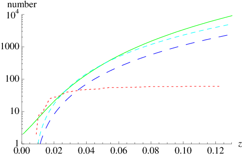
As can be seen this simple estimate is in agreement with the more complete analysis: current data are effected by correlated errors much more so than GAIA and LSST, which will be practically uneffected by correlations. In other words, under the assumption of a volume weighted redshift distribution for the SNe, GAIA and LSST can rely on the much higher redshift data to constrain our peculiar motion, as these are considerably less affected by PV correlations.

To summarize, we have used SALT calibrated SNe data to estimate the motion of he solar system. As seen from Table 1 the error bars are under-estimated by about 50% if the correlations in the peculiar velocity are not accounted for.

We now compare our findings to previous published results. In Bonvin et al. 2006 they used 44 SALT calibrated SNe. They only allowed $\{l,b,v_{O}\}$ to vary and all the other parameters where fixed to standard values. They did not account for correlations in the peculiar velocities. They found $v_{0}=405\pm 192$km/s which is compatible with our result.

In Jha et al. 2007 they used 69 SNe with $z\in\{0.005,0.025\}$. They also only allowed $\{l,b,v_{O}\}$ to vary. Additionally, they used MLCS2k2 to calibrate the data, rather than the SALT method. They also did not account for the correlations in the peculiar velocities. They evaluated the motion of the local group and found $\{l,b,v_{O}\}=\{258\pm 18^{\circ},51\pm 12^{\circ},541\pm 75{\rm km/s}\}$. Our local group velocity results, which are listed in Table 1, are compatible with those of Jha et al. 2007 but, even when we don’t take into account the correlations in the peculiar velocities, our error on the magnitude of $v_{0}$ is about 80% larger than that of Jha et al. 2007 study. This is due to several factors. They had a lower redshift limit than us: 0.005 vs. 0.0076. One of the reasons we did not go to such a low redshift is that the peculiar velocities (including the motion of our solar system) become of order the Hubble expansion. This means that the motion of our solar system has a high signal (hence the low error bars obtained by Jha et al. 2007) but one can no longer use Eq. (13) to evaluate the effects of peculiar velocity on the luminosity distance. It would be possible to use a higher order version of Eq. (13) but this was not done by Jha et al. 2007 and so their results will have an additional unreported systematic error due to the induced luminosity change being calculated incorrectly. Also, the extra very low redshift SNe that were used are dominated by SNe that are too close together to model the correlations in the peculiar velocity using linear theory, Eq. (15). Overall, our results are the only ones that take into account the correlations in peculiar velocities and account for the uncertainties in the cosmological and calibration parameters.

We also made forecasts for the GAIA and LSST surveys, assuming volume weighting for the redshift distribution. We found that the error bars will be about 4 times smaller than those of current data, but still not competitive with those from the CMB by a factor of $\sim 10$ (assuming that the CMB dipole is due to our local motion). Also, for GAIA and especially LSST we found that correlations had little effect as most of the signal came from higher redshifts where the correlations are almost negligible for the sample sizes considered.

In future work, we plan to test the techniques we have used in this paper against simulated SNe surveys generated from N-body simulations. These will test the assumptions that go into our data modeling - most importantly the effect of non-linearities (Haugboelle et al. 2006).

In Watkins & Feldman 2007 it was shown that the large scale properties (bulk flow and shear (Kaiser 1991; Jaffe & Kaiser 1995)) of the peculiar velocity field derived from a low redshift sample of 73 SNe was consistent with the bulk flow and shear of the velocity field derived from the SFI, ENEAR, and SBF surveys. It would be interesting to combine all these surveys together (with SFI replaced by SFI++ (Springob et al. 2007)) to estimate the solar system velocity with respect to the CMB and put robust limits on the intrinsic CMB dipole.

We thank Francesco Calura, Mark Sullivan, Licia Verde, and Joe Zuntz for helpful discussions. CG is funded by the Beecroft Institute for Particle Astrophysics and Cosmology, KL by a Glasstone research fellowship, and AS by Oxford Astrophysics and the Berkeley Center for Cosmological Physics.

References

- Belokurov & Evans (2003) Belokurov V., Evans N. W., 2003, MNRAS, 341, 569, \hrefhttp://arxiv.org/abs/astro-ph/0210570astro-ph/0210570
- Bonvin et al. (2006) Bonvin C., Durrer R., Gasparini M. A., 2006, Phys. Rev., D73, 023523, \hrefhttp://arxiv.org/abs/astro-ph/0511183astro-ph/0511183
- Bonvin et al. (2006) Bonvin C., Durrer R., Kunz M., 2006, Phys. Rev. Lett., 96, 191302, \hrefhttp://arxiv.org/abs/astro-ph/0603240astro-ph/0603240
- Cooray & Caldwell (2006) Cooray A., Caldwell R. R., 2006, Phys. Rev., D73, 103002, \hrefhttp://arxiv.org/abs/astro-ph/0601377astro-ph/0601377
- Dale & Giovanelli (2000) Dale D. A., Giovanelli R., 2000, in Courteau S., Willick J., eds, Cosmic Flows Workshop Vol. 201 of Astronomical Society of the Pacific Conference Series, The Convergence Depth of the Local Peculiar Velocity Field. pp 25–+, \hrefhttp://adsabs.harvard.edu/abs/2000ASPC..201…25DADS
- Dodelson (2003) Dodelson S., 2003, Modern cosmology. Academic Press, \hrefhttp://adsabs.harvard.edu/abs/2003moco.book…..DADS
- Eisenstein & Hu (1998) Eisenstein D. J., Hu W., 1998, ApJ, 496, 605, \hrefhttp://arxiv.org/abs/astro-ph/9709112astro-ph/9709112
- Erdogdu et al. (2006) Erdogdu P., et al., 2006, MNRAS, 368, 1515, \hrefhttp://arxiv.org/abs/astro-ph/0507166astro-ph/0507166
- Freedman et al. (2001) Freedman W. L., et al., 2001, ApJ, 553, 47, \hrefhttp://arxiv.org/abs/astro-ph/0012376astro-ph/0012376
- Gelman & Rubin (1992) Gelman A., Rubin D., 1992, Stat. Sci., 7, 457
- Gordon et al. (2007) Gordon C., Land K., Slosar A., 2007, Physical Review Letters, 99, 081301, \hrefhttp://adsabs.harvard.edu/abs/2007PhRvL..99h1301GADS, \hrefhttp://arxiv.org/abs/arXiv:0705.1718arXiv:0705.1718
- Gordon & Trotta (2007) Gordon C., Trotta R., 2007, \hrefhttp://arxiv.org/abs/arXiv:0706.3014 [astro-ph]arXiv:0706.3014 [astro-ph]
- Gorski (1988) Gorski K., 1988, ApJ, 332, L7
- Groth et al. (1989) Groth E. J., Juszkiewicz R., Ostriker J. P., 1989, ApJ, 346, 558
- Guy et al. (2005) Guy J., Astier P., Nobili S., Regnault N., Pain R., 2005, \hrefhttp://arxiv.org/abs/astro-ph/0506583astro-ph/0506583
- Haugboelle et al. (2006) Haugboelle T., et al., 2006, \hrefhttp://arxiv.org/abs/astro-ph/0612137astro-ph/0612137
- Hinshaw et al. (2007) Hinshaw G., et al., 2007, ApJS, 170, 288, \hrefhttp://arxiv.org/abs/astro-ph/0603451astro-ph/0603451
- Hui & Greene (2006) Hui L., Greene P. B., 2006, Phys. Rev., D73, 123526, \hrefhttp://arxiv.org/abs/astro-ph/0512159astro-ph/0512159
- Jaffe & Kaiser (1995) Jaffe A. H., Kaiser N., 1995, ApJ, 455, 26, \hrefhttp://adsabs.harvard.edu/abs/1995ApJ…455…26JADS, \hrefhttp://arxiv.org/abs/arXiv:astro-ph/9408046arXiv:astro-ph/9408046
- Jha et al. (2007) Jha S., Riess A. G., Kirshner R. P., 2007, ApJ, 659, 122, \hrefhttp://arxiv.org/abs/astro-ph/0612666astro-ph/0612666
- Kaiser (1991) Kaiser N., 1991, ApJ, 366, 388, \hrefhttp://adsabs.harvard.edu/abs/1991ApJ…366..388KADS
- Kirkman et al. (2003) Kirkman D., Tytler D., Suzuki N., O’Meara J. M., Lubin D., 2003, ApJS, 149, 1, \hrefhttp://arxiv.org/abs/astro-ph/0302006astro-ph/0302006
- Langlois (1996) Langlois D., 1996, Phys. Rev., D54, 2447, \hrefhttp://arxiv.org/abs/gr-qc/9606066gr-qc/9606066
- Langlois & Piran (1996) Langlois D., Piran T., 1996, Phys. Rev., D53, 2908, \hrefhttp://arxiv.org/abs/astro-ph/9507094astro-ph/9507094
- Lewis & Bridle (2002) Lewis A., Bridle S., 2002, Phys. Rev. D, 66, 103511
- Lewis et al. (2000) Lewis A., Challinor A., Lasenby A., 2000, ApJ, 538, 473, \hrefhttp://arxiv.org/abs/astro-ph/9911177astro-ph/9911177
- Loeb & Narayan (2007) Loeb A., Narayan R., 2007, \hrefhttp://arxiv.org/abs/arXiv:0711.3809 [astro-ph]arXiv:0711.3809 [astro-ph]
- Lynden-Bell et al. (1989) Lynden-Bell D., Lahav O., Burstein D., 1989, MNRAS, 241, 325, \hrefhttp://adsabs.harvard.edu/abs/1989MNRAS.241..325LADS
- Neill et al. (2007) Neill J. D., Hudson M. J., Conley A., 2007, \hrefhttp://arxiv.org/abs/arXiv:0704.1654 [astro-ph]arXiv:0704.1654 [astro-ph]
- Pyne & Birkinshaw (2004) Pyne T., Birkinshaw M., 2004, MNRAS, 348, 581, \hrefhttp://arxiv.org/abs/astro-ph/0310841astro-ph/0310841
- Riess et al. (1995) Riess A. G., Press W. H., Kirshner R. P., 1995, ApJ, 445, L91, \hrefhttp://arxiv.org/abs/astro-ph/9412017astro-ph/9412017
- Sasaki (1987) Sasaki M., 1987, MNRAS, 228, 653
- Silberman et al. (2001) Silberman L., Dekel A., Eldar A., Zehavi I., 2001, ApJ, 557, 102, \hrefhttp://arxiv.org/abs/astro-ph/0101361astro-ph/0101361
- Spergel et al. (2006) Spergel D. N., et al., 2006, \hrefhttp://arxiv.org/abs/astro-ph/0603449astro-ph/0603449
- Springob et al. (2007) Springob C. M., Masters K. L., Haynes M. P., Giovanelli R., Marinoni C., 2007, Astrophys. J. S., 172, 599, \hrefhttp://adsabs.harvard.edu/abs/2007ApJS..172..599SADS, \hrefhttp://arxiv.org/abs/arXiv:0705.0647arXiv:0705.0647
- Strauss et al. (1992) Strauss M. A., Yahil A., Davis M., Huchra J. P., Fisher K., 1992, ApJ, 397, 395, \hrefhttp://adsabs.harvard.edu/abs/1992ApJ…397..395SADS
- Sugiura et al. (1999) Sugiura N., Sugiyama N., Sasaki M., 1999, Progress of Theoretical Physics, 101, 903, \hrefhttp://adsabs.harvard.edu/abs/1999PThPh.101..903SADS
- Tegmark et al. (1997) Tegmark M., Taylor A., Heavens A., 1997, ApJ, 480, 22, \hrefhttp://arxiv.org/abs/astro-ph/9603021astro-ph/9603021
- Turner (1991) Turner M. S., 1991, Phys. Rev. D, 44, 3737, \hrefhttp://adsabs.harvard.edu/abs/1991PhRvD..44.3737TADS
- Wang et al. (2005) Wang L., Pinto P. A., Zhan H., 2005, in Bulletin of the American Astronomical Society Vol. 37 of Bulletin of the American Astronomical Society, LSST Supernova Cosmology. pp 1202–+
- Wang et al. (1998) Wang Y., Spergel D. N., Turner E. L., 1998, ApJ, 498, 1, \hrefhttp://arxiv.org/abs/astro-ph/9708014astro-ph/9708014
- Watkins & Feldman (2007) Watkins R., Feldman H. A., 2007, \hrefhttp://arxiv.org/abs/astro-ph/0702751astro-ph/0702751
- Yahil et al. (1977) Yahil A., Tammann G. A., Sandage A., 1977, ApJ, 217, 903, \hrefhttp://adsabs.harvard.edu/abs/1977ApJ…217..903YADS