跳到论文正文
W Papers独立论文阅读器 arXiv:0711.4187 论文正文 计算阅读时间 · 0%
引用这篇论文根据当前论文元数据生成,正式投稿前建议核对。


License: arXiv.org perpetual non-exclusive license
arXiv:0711.4187v3 [math.SG] 09 Feb 2010

Floer trajectories with immersed nodes and scale-dependent gluing Thanks: Y.-G. Oh is partially supported by the NSF grant # DMS 0503954

Yong-Geun Oh Address: Department of Mathematics, University of Wisconsin-Madison, Madison, WI, 53706 & Korea Institute for Advanced Study, Seoul, Korea Email address: oh@math.wisc.edu and Ke Zhu Address: Department of Mathematics, University of Wisconsin-Madison, Madison, WI, 53706 Email address: kzhu@math.wisc.edu
Date: Revision, January 6, 2010
Abstract.

Development of pseudo-holomorphic curves and Floer homology in symplectic topology has led to moduli spaces of pseudo-holomorphic curves consisting of both “smooth elements” and “spiked elements”, where the latter are combinations of JJ-holomorphic curves (or Floer trajectories) and gradient flow line segments. In many cases the “spiked elements” naturally arise under adiabatic degeneration of “smooth elements” which gradually go through thick-thin decomposition. The reversed process, the recovering problem of the “smooth elements” from “spiked elements” is recently of much interest.

In this paper, we define an enhanced compactification of the moduli space of Floer trajectories under Morse background using the adiabatic degeneration and the scale-dependent gluing techniques. The compactification reflects the 1-jet datum of the smooth Floer trajectories nearby the limiting nodal Floer trajectories arising from adiabatic degeneration of the background Morse function. This paper studies the gluing problem when the limiting gradient trajectories has length zero through a renomalization process. The case with limiting gradient trajectories of non-zero length will be treated elsewhere.

An immediate application of our result is a complete proof of the isomorphism property of the PSS map: A proof of this isomorphism property was outlined by Piunikhin-Salamon-Schwarz [PSS] in a way somewhat different from the current proof in its details. This kind of scale-dependent gluing techniques was initiated in [FOOO07] in relation to the metamorphosis of holomorphic polygons under Lagrangian surgery and is expected to appear in other gluing and compactification problem of pseudo-holomorphic curves that involves ‘adiabatic’ parameters or rescaling of the targets.

1. Introduction

Development of pseudo-holomorphic curves and Floer homology in symplectic geometry has led to moduli spaces consisting of both “smooth elements” and “spiked elements”, where the latter are combinations of JJ-holomorphic curves (or Floer trajectories) and gradient flow segments. For example, they appear in the generalized holomorphic building in symplectic field theory [BEHWZ], in the cluster complex [CL], and even earlier in the works [Fu2], [Oh2], [PSS], [Sc1] and [MT]. In many cases the “spiked elements” naturally arise from adiabatic degeneration of “smooth elements” which gradually decompose into “thick parts” and “thin parts”.

The adiabatic degeneration and its reversed process of the type studied in this paper has appeared in [FOh], [Ek] and [R]. The paper [SW] studied another type of adiabatic degeneration in a different context. All these papers are, however, restricted to the case without quantum contribution, i.e, without bubbling phenomenon. The papers [Oh7, Oh5] and [MT] studied adiabatic degeneration with quantum contribution close to the one studied in this paper. However the recovering problem was only mentioned and left as a future work in [Oh2], [MT].

Part of the difficulty for the recovering problem lies in finding good local models near the junction points where the JJ-holomorphic curve and gradient flow intersect. It turns out the derivative information of the JJ-holomorphic curve and the gradient flow at the junction point is needed to determine the local model. Besides a good local model, appropriate Fredholm theory and implicit function theorem are needed in order to glue the “spiked elements” to “smooth elements” in a controlled way to reflect the adiabatic degeneration. It turns out that the scale-dependent gluing technique carried out in chapter 10 of [FOOO07] in relation to metamorphosis of JJ-holomorphic polygon under the Lagrangian surgery, which treats a small region near the junction point as about the same size as the original target manifold, is needed to retain the geometric features of the local model under the perturbation via implicit function theorem. Large part of the analysis used in this paper is motivated by those in [FOOO07].

1.1. Adiabatic degeneration of Floer trajectories

In this paper, we study the adiabatic degeneration of maps u:ℝ×S1→Mu:{\mathbb{R}}\times S^{1}\to M satisfying the following 1-parameter (0<ε<ε00<\varepsilon<\varepsilon_{0}) family of Floer equations:

(d​u+PKε​(u))Jε(0,1)=0 or equivalently ​∂¯Jε​(u)+(PKε)Jε(0,1)​(u)=0,(du+P_{K_{\varepsilon}}(u))^{(0,1)}_{J_{\varepsilon}}=0\quad\mbox{ or equivalently }\,{\overline{\partial}}_{J_{\varepsilon}}(u)+(P_{K_{\varepsilon}})_{J_{\varepsilon}}^{(0,1)}(u)=0, (1.1)

We refer to Section 3 for detailed exposition of (1.1), the invariant form of the Floer equation. The expression of the degenerating Hamiltonian Kε:ℝ×S1×M→ℝK_{\varepsilon}:{\mathbb{R}}\times S^{1}\times M\to{\mathbb{R}} is given by

Kε​(τ,t,x)={κε+​(τ)⋅H⁡(t,x)for ​τ≥R⁡(ε)ρε​(τ)⋅ε​f​(x)for ​|τ|≤R⁡(ε)κε−​(τ)⋅H⁡(t,x)for ​τ≤−R⁡(ε)K_{\varepsilon}(\tau,t,x)=\begin{cases}\kappa_{\varepsilon}^{+}(\tau)\cdot H(t,x)\quad&\mbox{for }\,\tau\geq R(\varepsilon)\\ \rho_{\varepsilon}(\tau)\cdot\varepsilon f(x)\quad&\mbox{for }\,|\tau|\leq R(\varepsilon)\\ \kappa_{\varepsilon}^{-}(\tau)\cdot H(t,x)\quad&\mbox{for }\,\tau\leq-R(\varepsilon)\end{cases} (1.2)

where κe±\kappa_{e}^{\pm} and ρε\rho_{\varepsilon} are suitable cut-off functions (See (5.32) for the precise definition.) This type of equations, for example, appears in the study of isomorphism property of the PSS map introduced in [PSS].

Roughly speaking, the adiabatic degeneration occurs because KεK_{\varepsilon} restricts to Morse function ε​f\varepsilon f on longer and longer cylinder [−R⁡(ε),R⁡(ε)]×S1[-R(\varepsilon),R(\varepsilon)]\times S^{1} in ℝ×S1{\mathbb{R}}\times S^{1}. A basic assumption that we put on this paper is that R⁡(ε)R(\varepsilon) satisfies

limε→0ε​R​(ε)=0.\lim_{\varepsilon\to 0}\varepsilon R(\varepsilon)=0. (1.3)

The general case of limε→0ε​R​(ε)=ℓ\lim_{\varepsilon\to 0}\varepsilon R(\varepsilon)=\ell for ℓ>0\ell>0 will be studied in a forthcoming paper [OZ2]. Under this assumption, it is proved in [Oh7, Oh5] and [MT] that as ε→0\varepsilon\to 0, a degenerating sequence of Floer trajectories converges to a nodal Floer trajectory denoted by (u−,u+)(u_{-},u_{+}). Descriptions of nodal Floer trajectories and immersed nodal points are now in order.

Let Σ˙+\dot{\Sigma}_{+} be the Riemann sphere with one marked point o+o_{+} and one positive puncture e+e_{+}. Choose analytical charts at o+o_{+} and at e+e_{+} on some neighborhoods O+O_{+} and E+E_{+} respectively, so that conformally O+\o+≅(−∞,0]×S1O_{+}\backslash o_{+}\cong(-\infty,0]\times S^{1}, and E+\e+≅[0,+∞)×S1E_{+}\backslash e_{+}\cong[0,+\infty)\times S^{1}. We use tt for the S1S^{1} coordinate and τ\tau for the ℝ{\mathbb{R}} coordinate. Then {−∞}×S1\{-\infty\}\times S^{1} and {+∞}×S1\{+\infty\}\times S^{1} correspond to o+o_{+} and e+e_{+} respectively.

We consider a vector-valued 1-form K+K_{+} on Σ˙\dot{\Sigma} with its values in the set h​a​m​(M,ω)ham(M,\omega) of Hamiltonian vector fields on (M,ω)(M,\omega), and Σ˙=ℂ​P1∖{e+,o+}≅ℂ∖{0}≅ℝ×S1\dot{\Sigma}={\mathbb{C}}P^{1}\setminus\{e_{+},o_{+}\}\cong{\mathbb{C}}\setminus\{0\}\cong{\mathbb{R}}\times S^{1}. We denote by (τ,t)(\tau,t) the standard coordinate on ℝ×S1{\mathbb{R}}\times S^{1}. With respect to this coordinates, we require K+K_{+} satisfy

{K+=0near​o+K+=H+​(t,x)​d​tnear​e+\left\{\begin{array}[]{rcll}K_{+}&=&0&\text{near}\;o_{+}\\ K_{+}&=&H_{+}(t,x)\,dt&\text{near}\;e_{+}\end{array}\right. (1.4)

H+:S1×M→ℝH_{+}:S^{1}\times M\to{\mathbb{R}} is a Hamiltonian function independent of the variable τ\tau.

Let z+:S1→Mz_{+}:S^{1}\to M be a nondegenerate periodic orbit of H+H_{+} and consider a finite energy solution u+:Σ˙→Mu_{+}:\dot{\Sigma}\to M of the Floer equation (1.1) associated to K+K_{+}. By the finite energy condition and since K+≡0K_{+}\equiv 0 near o+o_{+}, u+u_{+} extends smoothly across o+o_{+} and can be regarded as a smooth map defined on ℂ{\mathbb{C}} that is holomorphic near the origin 0∈ℂ0\in{\mathbb{C}}.

Similarly we consider 1-form K−K_{-} on Σ˙\dot{\Sigma} and Σ˙=ℂ​P1∖{o−,e−}≅ℂ∖{0}≅ℝ×S1\dot{\Sigma}={\mathbb{C}}P^{1}\setminus\{o_{-},e_{-}\}\cong{\mathbb{C}}\setminus\{0\}\cong{\mathbb{R}}\times S^{1}. We denote by (τ,t)(\tau,t) the standard coordinate on ℝ×S1{\mathbb{R}}\times S^{1} so that +∞+\infty corresponds to o−o_{-} and −∞-\infty to e−e_{-}. With respect to this coordinates, we require K+K_{+} satisfy

{K−=0near​o−K−=H−​(t,x)​d​tnear​e−\left\{\begin{array}[]{rcll}K_{-}&=&0&\text{near}\;o_{-}\\ K_{-}&=&H_{-}(t,x)\,dt&\text{near}\;e_{-}\end{array}\right. (1.5)

H±:S1×M→ℝH_{\pm}:S^{1}\times M\to{\mathbb{R}} are a pair of Hamiltonian functions independent of the variable τ\tau. Let z±:S1→Mz_{\pm}:S^{1}\to M be a nondegenerate periodic orbit of H±H_{\pm} and its lifting [z±,w±][z_{\pm},w_{\pm}] of z±z_{\pm}.

A nodal Floer trajectory is, by definition, the gluing u−​#​u+u_{-}\#u_{+} at u−​(o−)=u+​(o+)u_{-}(o_{-})=u_{+}(o_{+}) where u±u_{\pm} are the solutions of the Floer equation associated to K±K_{\pm} respectively. We say that a nodal point of u−​#​u+u_{-}\#u_{+} is immersed if u±u_{\pm} are immersed at o±o_{\pm} respectively.

One of the main results of the paper is the following enhanced compactification theorem in Section 12 (Theorem 12.10) for gluing and its surjectivity:

Theorem 1.1.

Suppose that u−,u+u_{-},\,u_{+} are immersed at the node

p=u−​(o−)=u+​(o+).p=u_{-}(o_{-})=u_{+}(o_{+}).

Let G​l​u​e​(u−,u+)Glue(u_{-},u_{+}) be the nodal Floer trajectory formed by u−u_{-} and u+u_{+} with nodal points p=u−​(o−)=u+​(o+)p=u_{-}(o-)=u_{+}(o_{+}). Suppose that unu_{n} converges to G​l​u​e​(u−,u+)Glue(u_{-},u_{+}) in level 0. Then there exists a subsequence uniu_{n_{i}} and a sequence εi→0\varepsilon_{i}\to 0 such that uniu_{n_{i}} converges to (u−,u+,u0)(u_{-},u_{+},u_{0}) in the {εi}\{\varepsilon_{i}\}-controlled way.

A more detailed description of the local model u0u_{0} above is in order now.

The convergence in level 0 is the usual Gromov convergence (Definition 12.6). The convergence in ε\varepsilon-controlled way is in Definition 12.9. Roughly speaking, we magnify suitable small neighborhood of the center of the neck of uniu_{n_{i}} to keep track of the degeneration in microscopic level, and in the limit we get a proper holomorphic curve in ℂn{\mathbb{C}}^{n} with asymptotic convergence to simple Reeb orbits γ−\gamma_{-} and γ+\gamma_{+} of the standard contact form λ\lambda on S2​n−1S^{2n-1} in the cylindrical end ℝ×(S2​n−1,λ){\mathbb{R}}\times(S^{2n-1},\lambda) of ℂn{\mathbb{C}}^{n}. Such a holomorphic curve can be identified as a degree 2 rational curve in ℂ​Pn{\mathbb{C}}P^{n} intersecting the hyperplane at infinity at two points x0x_{0} and x∞x_{\infty}. We have the following classification result of such rational curves (Proposition 6.1):

Proposition 1.2.

Fix a hyperplane HH in ℂ​Pn{\mathbb{C}}P^{n} and two points x0,x∞∈Hx_{0},\,x_{\infty}\in H. Then there exists a unique, modulo the action of A​u​t​(ℂ​Pn,H)Aut({\mathbb{C}}P^{n};H), rational curve passing through x0,x1x_{0},\,x_{1} of degree 2 which is the group of automorphisms of ℂ​Pn{\mathbb{C}}P^{n} fixing HH.

We can give an explicit formula for such rational curves. (See Remark 6.3 for such formula.) We refer to Theorem 6.2 for the explanation how this proposition can be used to provide the local model u0u_{0}. (Strictly speaking the microscopic adiabatic limit has some remnant from the background small Morse function ε​f\varepsilon f put in the middle of KεK_{\varepsilon} (5.32) above and is a proper holomorphic curve perturbed by a linear vector τ∇f(p)\tau\nabla f(p), i.e., has the form u0+τ∇f(p)u_{0}+\tau\nabla f(p) See Proposition 7.4.)

We call (u−,u+,u0)(u_{-},u_{+},u_{0}) an enhanced nodal Floer trajectory. For a given enhanced nodal Floer trajectory, we glue a 1-parameter family of smooth Floer trajectories and show that they are all possible nearby smooth Floer trajectories according to the topology defined by the above enhanced convergence. (See Theorem 10.19 for the precise statement.)

The equation (1.1) is nothing but a coordinate free expression of the equation arising in the framework of the PSS map described in [PSS]. A key step during the PSS scheme of proof of the isomorphism property is to resolve the nodal Floer trajectory to a 1-parameter family of smooth Floer trajectories. Unlike the smoothing trajectories obtained via the more conventional gluing outlined in [PSS], [MS] (see also [Lu]), our resolved Floer trajectories is more closely tied to the limiting configurations arising through adiabatic degeneration in that they are aligned in the gradient flow direction near the node and is related to the disk-flow-disk elements.

Remark 1.3.

As far as we know, the detail of a key gluing result needed in the proof of isomorphism property of the PSS map announced in [PSS] has not been given yet in any previous literature and our paper is the first one that provides a full detail of the proof of isomorphism property of the PSS map. Our proof uses a somewhat possibly “overkilled” gluing result obtained in Theorem 12.10 and 10.19: Although we did not check it, it is conceivable that one might be able to write down a proof, without rescaling target manifolds, following the more standard approach of Floer’s gluing [Fl1]. However we strongly believe that to materialize such a proof one will still need to assume that nodes are immersed as we do in the present paper. Such a requirement has not been addressed in the proposed PSS scheme in [PSS] or in any other existing literature related to it. We refer to the next subsection for more discussion on the non-triviality of this gluing theorem involved in the PSS scheme. See also Remark 5.6.

In this paper, we take the PSS framework as a test case to apply our scale-dependent gluing scheme thereto because the PSS picture appears as the simplest case for an adiabatic degeneration yet manifests the general technique. Our gluing scheme can also be applied to other context such as in the story told in [Oh2] where the adiabatic degeneration of holomorphic polygons under the total collapse of kk Lagrangian graphs Graph⁡d​fi\operatorname{Graph}df_{i}, i=1,⋯,ki=1,\cdots,k in a Darboux neighborhood of a given Lagrangian submanifold L⊂ML\subset M was outlined which involves configurations of holomorphic curves joined by gradient trajectories of kk different Morse functions in a general symplectic manifold (M,ω)(M,\omega). In this general case there are non-constant holomorphic spheres or discs around unlike the case of cotangent bundle studied in [FOh]. This is a subject of future study [OZ2].

1.2. Nodal Floer trajectories with immersed nodes

Temporarily we denote by ℳε{\mathcal{M}}_{\varepsilon} the general moduli space parameterized by ε\varepsilon for −ε0≤ε≤ε0-\varepsilon_{0}\leq\varepsilon\leq\varepsilon_{0} with some phase change at ε=0\varepsilon=0. We will focus on the one that appears in the above mentioned PSS scheme but the same story can be applied to more general setting. In relation to the scheme of proof of the isomorphism property of the PSS map, for example, one would like to prove a certain parametrized moduli space

ℳp​a​r​a:=⋃−ε0≤ε≤ε0ℳε→[−ε0,ε0]{\mathcal{M}}^{para}:=\bigcup_{-\varepsilon_{0}\leq\varepsilon\leq\varepsilon_{0}}{\mathcal{M}}_{\varepsilon}\to[-\varepsilon_{0},\varepsilon_{0}]

defines a piecewise smooth compact cobordism between ℳ−ε0{\mathcal{M}}_{-\varepsilon_{0}} and ℳε0{\mathcal{M}}_{\varepsilon_{0}}: there occurs a ‘phase change’ at ε=0\varepsilon=0. Due to the ‘phase change’ at ε=0\varepsilon=0, one needs to prove a bi-collar theorem of ℳ0⊂ℳp​a​r​a{\mathcal{M}}_{0}\subset{\mathcal{M}}^{para} to materialize the PSS-scheme. From −ε0-\varepsilon_{0} to 00, one can construct the left one-sided collar by finite dimensional differential topology (See Section 9). On the other hand, for the right one-sided collar over [0,ε0][0,\varepsilon_{0}], [PSS] attempts to produce the collar by a ‘standard gluing method’ of ‘some’ perturbed Cauchy Riemann equation. More specifically, [PSS] attempts to produce a diffeomorphism

⋃0≤ε≤ε0ℳε≅ℳ0×[0,ε0]\bigcup_{0\leq\varepsilon\leq\varepsilon_{0}}{\mathcal{M}}_{\varepsilon}\cong{\mathcal{M}}_{0}\times[0,\varepsilon_{0}]

for a sufficiently small ε0>0\varepsilon_{0}>0. However the details of this gluing theorem are given neither in [PSS], [Lu] nor in the recent book [MS]. As far as the authors understand, construction of this diffeomorphism is not as standard as [PSS], [MS] indicated.

The main result of the present paper is to construct this one-sided collar, at ε=0\varepsilon=0 (not at ∞\infty), by producing a one-parameter family of Floer trajectories out of the nodal Floer trajectories (out of ℳ0{\mathcal{M}}_{0}) by the adiabatic degeneration [Oh7, Oh5], [MT] and a scale-dependent gluing method. We would like to emphasize that due to the phase change at ε=0\varepsilon=0 the standard gluing theorem of parameterized moduli space over ε\varepsilon cannot be applied either here.

If we only consider the usual stable map convergence a ε→0\varepsilon\to 0, we only see the standard nodal Floer trajectories as a degenerate limit when we ignore bubbling-off-spheres. But to recover the nearby resolved Floer trajectories for ε>0\varepsilon>0 and construct the above mentioned one-sided collar, we need extra 1-jet data that is lost into the node during the standard stable map convergence. For this purpose, it is essential to assume that nodal points are immersed. For the purpose of completing the proof of isomorphism property of the PSS map, consideration of such nodal Floer trajectories will be sufficient.

Let [z±,w±][z_{\pm},w_{\pm}] be periodic orbits with caps of H±H_{\pm} respectively. We denote by

ℳs​t​a​n​dn​o​d​a​l​([z−,w−],[z+,w+],(K,J)){\mathcal{M}}_{stand}^{nodal}([z_{-},w_{-}],[z_{+},w_{+}];(K,J))

the set of nodal Floer trajecotories in class B∈π2​(z−,z+)B\in\pi_{2}(z_{-},z_{+}) that satisfies

[w−]​#​B​#​[w+]=0.[w_{-}]\#B\#[w_{+}]=0.

Here π2​(z−,z+)\pi_{2}(z_{-},z_{+}) is the set of homotopy class of maps w:[0,1]×S1→Mw:[0,1]\times S^{1}\to M satisfying w⁡(0,t)=z−​(t)w(0,t)=z_{-}(t), w​(1,t)=z+​(t)w(1,t)=z_{+}(t). Note that the gluing u−​#​u+u_{-}\ \#u_{+} canonically assigns a class in π2​(z−,z+)\pi_{2}(z_{-},z_{+}). A general index theorem [SZ] says that the virtual dimension of the moduli space ℳs​t​a​n​dn​o​d​a​l​([z−,w−],[z+,w+],(K,J)){\mathcal{M}}_{stand}^{nodal}([z_{-},w_{-}],[z_{+},w_{+}];(K,J)) is given by

μH−​([z−,w−])−μH+​([z+,w+])\mu_{H_{-}}([z_{-},w_{-}])-\mu_{H_{+}}([z_{+},w_{+}])

where μH​([z,w])\mu_{H}([z,w]) is the Conley-Zehnder index [CZ] of the periodic orbit zz with cap ww associated to the Hamiltonian HH. The sign conventions of [CZ], [SZ] are different from those used in the present paper one way or the other. We refer to Appendix of [Oh6] for a discussion of the index formula in the convention used in the present paper.

The following theorem enable us to consider only the nodal Floer trajectories with immersed node for the purpose of proving isomorphism property of the PSS map.

Theorem 1.4.

Let (K±,J±)(K_{\pm},J_{\pm}) be a Floer datum with the asymptotic Hamiltonian H±H_{\pm}. Suppose that

μH−​([z−,w−])−μH+​([z+,w+])<2​n−1.\mu_{H_{-}}([z_{-},w_{-}])-\mu_{H_{+}}([z_{+},w_{+}])<2n-1.

Then there exists a dense subset of 𝒥ω{\mathcal{J}}_{\omega} consisting of JJ’s such that for any quintuple

(u−,u+,r−,r+)∈ℳs​t​a​n​dn​o​d​a​l​([z−,w−],[z+,w+],(K,J))(u_{-},u_{+},r_{-},r_{+})\in{\mathcal{M}}_{stand}^{nodal}([z_{-},w_{-}],[z_{+},w_{+}];(K,J))

with u−​(r−)=u+​(r+)u_{-}(r_{-})=u_{+}(r_{+}), r−r_{-} and r+r_{+} are immersed points of u−u_{-} and u+u_{+} respectively, and

[d​u−​(r−)]≠[d​u+​(r+)] in ​ℙ​(Tx​M)[du_{-}(r_{-})]\neq[du_{+}(r_{+})]\quad\mbox{ in }\,{\mathbb{P}}(T_{x}M)

with x=u−​(r−)=u+​(r+)x=u_{-}(r_{-})=u_{+}(r_{+}). The same holds for a one parameter family of such (K±,J±)(K_{\pm},J_{\pm}).

In particular, these hold when μ⁡([z−,w−])−μ⁡([z+,w+])=0\mu([z_{-},w_{-}])-\mu([z_{+},w_{+}])=0, or −1-1.

1.3. Related works and organization of the content

Our gluing theorem involves two moduli spaces in different scales. This kind of gluing theorem first appeared in [FOh] in symplectic geometry, in which Fukaya and Oh glued holomorphic discs with boundary punctures at the intersections of several gradient trajectories of different Morse functions after they are shrunk with a prescribed scale depending on degeneration parameter ε\varepsilon. Another scale-dependent gluing theorem has been also used in [FOOO07] in relation to the Lagrangian surgery and metamorphosis of holomorphic polygons. Furthermore the kind of analysis that has been used for the analysis of proper pseudo-holomorphic curves in symplectic manifolds with cylindrical ends [Ho], [HWZ1, HWZ2, HWZ4] also plays a crucial role in our analysis. This analysis is further complicated by the fact that we have to work out the relevant estimates in the setting of asymptotically cylindrical ends on incomplete manifolds, especially in the proof of surjectivity of the gluing.

Finally it would be worthwhile to mention that the analysis given in the present paper is a first step towards a full understanding of the conjectural picture described in [Oh2] which would require this type of scale-dependent gluing theorem of pseudo-holomorphic curves under the background Morse function, or twisted by the Hamiltonian flow of a Morse function. Based on the argument of adiabatic degeneration, the senior author indicated that ‘homology’ of the quantum chain complex will be isomorphic to that of the Floer complex, if they defined. Study of some related collapsing degenerations has been carried out by the senior author in [Oh7, Oh5] and by Mundet i Rierra and Tian [MT].

We would like to mention one potential application of our gluing scheme. In [FOOO07], scale-dependent gluing was used to compare the moduli space of JJ-holomorphic triangles ending on 3 Lagrangian submanifolds (L0,L1,L2)(L_{0},L_{1},L_{2}) and the moduli space of JJ-holomorphic 2-gons ending on two Lagrangian submanifolds (L0,L1​#λ​L2)(L_{0},L_{1}\#_{\lambda}L_{2}), where L1​#λ​L2L_{1}\#_{\lambda}L_{2} is obtained by Lagrangian surgery from L1L_{1} and L2L_{2}. Similar to the Lagrangian surgery to smooth the singular Lagrangian submanifolds L1∪L2L_{1}\cup L_{2} to L1​#λ​L2L_{1}\#_{\lambda}L_{2}, we expect our scale-dependent gluing can be used to understand JJ-holomorphic curves in singular target spaces, or its change when the target manifold undergoes some surgery.

A brief summary of each part of the paper is in order. In Part I, we set-up a new geometric framework which addresses an enhancement of the description of standard nodal Floer trajectories. In this enhancement, it is essential to assume that the nodes of nodal Floer trajectories are immersed and to insert suitable local models at the nodes in 1-jet level, so we prove Theorem 1.4 (Theorem 5.4).

In Part II, we carry out a scale-dependent gluing analysis to glue two outer pseudo-holomorphic curves and the local model in different scale which is somewhat reminiscent of the ones in [FOh], [FOOO07]. In this scale-dependent analysis, the immersion property of nodal points and a proper choice of scales of neck-stretching relative to the adiabatic parameter is essential.

In Part III, we combine these with the standard deformation-cobordism argument to explain how our gluing theorem can be used to give a proof of the isomorphism property of the PSS map.

Y.-G. Oh would like to thank K. Fukaya, H. Ohta and K. Ono for the collaboration of the book [FOOO07]. A large part of analysis carried out in Part II of the current work is much influenced by the scale-dependent gluing analysis given in Chapter 10 of the book. He also thanks Bumsig Kim for the help in the argument used in the proof of Proposition 6.1, and National Institute for Mathematical Sciences(NIMS) in Korea for providing its financial support and office space during the fall of 2009 where the final version of the present paper is finished. K. Zhu would like to thank the math department of University of Wisconsin-Madison and Korea Institute of Advanced Study for the nice environment, where most of his research was carried out.

Finally, but not the least, we would like to express our deep gratitude to the anonymous referee for pointing out many inaccuracies in our presentation and providing many suggestions to improve the presentation of the paper.

2. Review of the classical Floer’s equation

Throughout this paper, (M,ω)(M,\omega) is a compact symplectic manifold. We will always identify S1S^{1} with ℝ/ℤ{\mathbb{R}}/{\mathbb{Z}} which in particular has the canonical marking 0(mod1)∈S10(\mod 1)\in S^{1}. Denote by S=ℝ×S1S={\mathbb{R}}\times S^{1} the infinite cylinder with the unique complex structure, denoted by jj. We denote by (τ,t)(\tau,t) be the associated cylindrical coordinates such that

τ+i​t,τ∈ℝ,t∈S1=ℝ/ℤ\tau+it,\quad\tau\in{\mathbb{R}},\,t\in S^{1}={\mathbb{R}}/{\mathbb{Z}}

provides the standard complex coordinates on SS identified with the quotient space S=ℂ/i​ℤS={\mathbb{C}}/i{\mathbb{Z}} which lifts to the standard coordinates z=e2​π​(τ+i​t)z=e^{2\pi(\tau+it)} on ℂ{\mathbb{C}}.

Let J=J⁡(τ,t)J=J(\tau,t) be a 2-parameter family of almost complex structures compatible with ω\omega for (τ,t)∈R×S1(\tau,t)\in R\times S^{1} satisfying the asymptotic condition

J(τ,t)≡J(±∞,t)for τ≥R+ and τ≤−R−J(\tau,t)\equiv J(\pm\infty,t)\quad\mbox{for $\tau\geq R_{+}$ and $\tau\leq-R_{-}$} (2.1)

for some R±≥0R_{\pm}\geq 0. Denote the set of all such JJ by 𝒥=𝒥ω\mathcal{J}={\mathcal{J}}_{\omega}, and by 𝒥ωc​y​l{\mathcal{J}}^{cyl}_{\omega} the set of such JJ’s independent of τ\tau.

Next we consider two parameter family of smooth functions on MM parameterized by (τ,t)∈ℝ×S1(\tau,t)\in{\mathbb{R}}\times S^{1}

H=H⁡(τ,t,x)H=H(\tau,t,x)

such that H⁡(τ,t,x)≡H±​(t,x)H(\tau,t,x)\equiv H_{\pm}(t,x) for τ≥R+\tau\geq R_{+} or τ≤R−\tau\leq R^{-}. We call HH cylindrical if HH is independent of τ\tau. For each given cylindrical HH, we consider the Hamilton equation

x˙=XH​(t,x),t∈S1,\dot{x}=X_{H}(t,x),\,t\in S^{1},

where XHX_{H} is the Hamiltonian vector field of HH, and denote by Per⁡H\operatorname{Per}H the set of one-periodic solutions z⁡(t)z(t), i.e., those satisfying z⁡(0)=z⁡(1)z(0)=z(1). We note that z⁡(t)z(t) can be written as z⁡(t)=ϕHt​(x)z(t)=\phi_{H}^{t}(x) for some x∈Mx\in M, where ϕHt\phi_{H}^{t} is the Hamiltonian flow for HH at time tt. Then z⁡(t)z(t) is periodic if and only if xx is a fixed point of the time-one map ϕH1\phi_{H}^{1} of XHX_{H}.

For each given periodic orbits z±​(t)z_{\pm}(t) at τ=±∞\tau=\pm\infty of H±H_{\pm} respectively, the Floer’s perturbed Cauchy Riemann equation associated to the pair (H,J)(H,J) has the form

{∂u∂τ+J⁡(∂u∂t−XH​(u))=0u⁡(−∞,t)=z−​(t),u⁡(∞,t)=z+​(t)\begin{cases}{\frac{\partial u}{\partial\tau}}+J\Big({\frac{\partial u}{\partial t}}-X_{H}(u)\Big)=0\\ u(-\infty,t)=z_{-}(t),\,u(\infty,t)=z_{+}(t)\end{cases} (2.2)

for a map u:ℝ×S1→Mu:{\mathbb{R}}\times S^{1}\to M. We call this equation Floer’s perturbed Cauchy-Riemann equation or simply as the perturbed Cauchy-Riemann equation (associated to the pair (H,J)(H,J)). This equation may be regarded as the negative gradient flow equation of an action functional defined on the Novikov covering space. The Floer theory largely relies on the study of the moduli spaces of finite energy solutions u:ℝ×S1→Mu:{\mathbb{R}}\times S^{1}\to M of the kind (14.5). The relevant energy function is given by

Definition 2.1.

For a given smooth map u:ℝ×S1→Mu:{\mathbb{R}}\times S^{1}\to M, we define the energy, denoted by E(H,J)​(u)E_{(H,J)}(u), of uu by

E(H,J)​(u)=12​∫(|∂u∂τ|Jt2+|​∂u∂t−XH​(u)|Jt2)​𝑑t​𝑑τ.E_{(H,J)}(u)=\frac{1}{2}\int\Big(\Big|{\frac{\partial u}{\partial\tau}}\Big|^{2}_{J_{t}}+\Big|{\frac{\partial u}{\partial t}}-X_{H}(u)\Big|_{J_{t}}^{2}\Big)\,dt\,d\tau.

The equation (14.5) has translational symmetry for the cylindrical pair (H,J)(H,J) and counting the isolated trajectories of such pair defines the Floer boundary map, and counting isolated trajectories of generic (non-cylindrical) pair defines the Floer chain map. This finishes the summary of Floer’s original set-up of the Floer homology.

When one considers the product structure on the Floer homology, one needs to consider general Riemann surfaces, Σ˙\dot{\Sigma} of genus zero with punctures. We denote by Σ\Sigma a closed Riemann surface, possibly with non-empty boundary ∂Σ\partial\Sigma, and Σ˙\dot{\Sigma} the corresponding punctured Riemann surface with a finite number of marked points in Int⁡Σ\operatorname{Int}\Sigma.

3. Invariant set-up of the Floer equation

In this section, we will formulate the set-up for the general Floer’s perturbed Cauchy-Riemann equation on compact Riemann surface with a finite number of punctures. This requires a coordinate-free framework of the equation.

3.1. Punctures with analytic coordinates

We start with the description of positive and negative punctures. Let Σ\Sigma be a compact Riemann surface with a marked point p∈Σp\in\Sigma. Consider the corresponding punctured Riemann surface Σ˙\dot{\Sigma} with an analytic coordinates z:D∖{p}→ℂz:D\setminus\{p\}\to{\mathbb{C}} on a neighborhood D∖{p}⊂Σ˙D\setminus\{p\}\subset\dot{\Sigma}. By composing zz with a linear translation of ℂ{\mathbb{C}}, we may assume z⁡(p)=0z(p)=0.

We know that D∖{p}D\setminus\{p\} is conformally isomorphic to both [0,∞)×S1[0,\infty)\times S^{1} and (−∞,0]×S1(-\infty,0]\times S^{1}.

  1. (1)

    We say that the pair (p;(D,z))(p;(D,z)) has a incoming cylindrical end (with analytic chart) if we have

    D=z−1​(D2​(1))D=z^{-1}(D^{2}(1))

    and are given by the biholomorphism

    (τ,t)∈S1×(−∞,0]↦e2​π​(τ+i​t)∈D2(1)∖{0}↦z−1∈D∖{p}.(\tau,t)\in S^{1}\times(-\infty,0]\mapsto e^{2\pi(\tau+it)}\in D^{2}(1)\setminus\{0\}\mapsto z^{-1}\in D\setminus\{p\}.

    We call the corresponding puncture p∈Σp\in\Sigma a positive puncture.

  2. (2)

    We say that the pair (p;(D,z))(p;(D,z)) has a outgoing cylindrical end (with analytic chart) if we have

    D=z−1​(D2​(1))D=z^{-1}(D^{2}(1))

    and are given by the biholomorphism

    (τ,t)∈S1×[0,∞)↦e−2​π​(τ+i​t)∈D2​(1)∖{0}↦z−1∈D∖{p}.(\tau,t)\in S^{1}\times[0,\infty)\mapsto e^{-2\pi(\tau+it)}\in D^{2}(1)\setminus\{0\}\mapsto z^{-1}\in D\setminus\{p\}.

    In this case, we call the corresponding puncture (p;(D,z))(p;(D,z)) a negative puncture (with analytic chart).

3.2. Hamiltonian perturbations

Now we describe the Hamiltonian perturbations in a coordinate free fashion. Such a description was given, for example, by Seidel in [Se2, Se3, MS].

Let Σ\Sigma be a compact Riemann surface and Σ˙\dot{\Sigma} denote Σ\Sigma with a finite number of punctures and analytic coordinates. We denote by 𝒥0,ω{\mathcal{J}}_{0,\omega} the set of almost complex structures that are cylindrical near the puncture with respect to the given analytic charts z=e±(2​π​(τ+i​t)CLOSEz=e^{\pm(2\pi(\tau+it)}. Define 𝒥Σ{\mathcal{J}}_{\Sigma} or 𝒥Σ˙{\mathcal{J}}_{\dot{\Sigma}} to be the set of maps J:Σ,Σ˙→𝒥0,ωJ:\Sigma,\,\dot{\Sigma}\to{\mathcal{J}}_{0,\omega} respectively.

We recall that the standard ∂¯{\overline{\partial}}-operator

∂¯J:u↦∂¯J​u:=d​u+J∘d​u∘j2{\overline{\partial}}_{J}:u\mapsto{\overline{\partial}}_{J}u:=\frac{du+J\circ du\circ j}{2}

defines a section of the vector bundle

ΩJ(0,1)​(Σ,M)→C∞​(Σ,M)\Omega^{(0,1)}_{J}(\Sigma,M)\to C^{\infty}(\Sigma,M)

where the fiber thereof at uu is given by the vector space

ΩJ(0,1)​(u∗​T​M):=C∞​(ΛJ(0,1)​(u∗​T​M))\Omega^{(0,1)}_{J}(u^{*}TM):=C^{\infty}(\Lambda_{J}^{(0,1)}(u^{*}TM))

where ΛJ(0,1)​(u∗​T​M)\Lambda_{J}^{(0,1)}(u^{*}TM) is the set of anti-JJ-linear maps from (T​Σ,j)→(T​M,J)(T\Sigma,j)\to(TM,J) lifting uu, or in other words, u∗​T​Mu^{*}TM-valued (0,1)(0,1)-forms on Σ\Sigma. Recall we have the decomposition

Ω1​(u∗​T​M)=ΩJ(1,0)​(u∗​T​M)⊕ΩJ(0,1)​(u∗​T​M).\Omega^{1}(u^{*}TM)=\Omega^{(1,0)}_{J}(u^{*}TM)\oplus\Omega^{(0,1)}_{J}(u^{*}TM).

In the cylindrical coordinates (τ,t)(\tau,t), the map

∂∂τ⌋(⋅):ΩJ(0,1)(u∗TM)→Ω0(u∗TM)=C∞(u∗TM)\frac{\partial}{\partial\tau}\rfloor(\cdot):\Omega^{(0,1)}_{J}(u^{*}TM)\to\Omega^{0}(u^{*}TM)=C^{\infty}(u^{*}TM)

defines a local isomorphism and the expression ∂u∂τ+J​∂u∂t{\frac{\partial u}{\partial\tau}}+J{\frac{\partial u}{\partial t}} in the Floer equation is nothing but

2​∂¯J​u​(∂∂τ).2{\overline{\partial}}_{J}u\left(\frac{\partial}{\partial\tau}\right).

We want to regard the perturbation term −J​XH​(u)-JX_{H}(u) in a similar way. It will be the value of the (0,1)(0,1)-part of some one-form PΣ˙​(u)∈Ω1​(u∗​T​M)P_{\dot{\Sigma}}(u)\in\Omega^{1}(u^{*}TM). Furthermore the term involves a Hamiltonian vector field, not a general vector field. We recall the exact sequence

0→ℝ→C∞​(M)→h​a​m​(M,ω)→00\to{\mathbb{R}}\to C^{\infty}(M)\to ham(M,\omega)\to 0

where h​a​m​(M,ω)ham(M,\omega) is the set of Hamiltonian vector fields on (M,ω)(M,\omega) and we assume that MM is compact and connected. This sequence canonically splits : we have the integration map

∫M:C∞​(M)→ℝ;h↦∫Mh​𝑑μ.\int_{M}:C^{\infty}(M)\to{\mathbb{R}}\,;\,h\mapsto\int_{M}h\,d\mu.

Therefore this induces a natural exact sequence

0→Ω1​(Σ,ℝ)→Ω1​(Σ,C∞​(M))→Ω1​(Σ,h​a​m​(M,ω))→0.0\to\Omega^{1}(\Sigma,{\mathbb{R}})\to\Omega^{1}(\Sigma,C^{\infty}(M))\to\Omega^{1}(\Sigma,ham(M,\omega))\to 0.

If we restrict the Hamiltonians to the mean-normalized ones, i.e., those in the kernel of the above integral map, we have the isomorphism

Ω1​(Σ,Cm∞​(M))≅Ω1​(Σ,h​a​m​(M,ω)).\Omega^{1}(\Sigma,C^{\infty}_{m}(M))\cong\Omega^{1}(\Sigma,ham(M,\omega)).

We denote Cm∞(M)=ker∫MC^{\infty}_{m}(M)=\ker\int_{M}.

Now let K∈Ω1​(Σ,C∞​(M))K\in\Omega^{1}(\Sigma,C^{\infty}(M)) and denote by PKP_{K} the corresponding one-form of Ω1​(Σ,h​a​m​(M,ω))\Omega^{1}(\Sigma,ham(M,\omega)). Then for each choice of ξ∈C∞​(T​Σ)\xi\in C^{\infty}(T\Sigma), K⁡(ξ){K(\xi)} gives a function on MM and so a Hamiltonian vector field PK​(ξ)=XK⁡(ξ)P_{K}(\xi)=X_{K(\xi)} on MM. In cylindrical coordinate (τ,t)(\tau,t), we want KK to satisfy

−2​(PK)(0,1)​(u)​(∂∂τ)=−J​XH​(u).-2(P_{K})^{(0,1)}(u)\left(\frac{\partial}{\partial\tau}\right)=-JX_{H}(u).

It is easy to check that one such choice of KK will be

K⁡(τ,t)=H⁡(t)​d​tK(\tau,t)=H(t)\,dt (3.1)

on the cylindrical ends for an arbitrary choice of HH.

Definition 3.1.

We call K∈Ω1​(Σ,C∞​(M))K\in\Omega^{1}(\Sigma,C^{\infty}(M)) cylindrical at the puncture p∈Σp\in\Sigma with analytic chart (D,z)(D,z), if it has the form

K⁡(τ,t)=H⁡(t)​d​tK(\tau,t)=H(t)\,dt

in D∖{p}D\setminus\{p\}. We denote by 𝒦Σ˙{\mathcal{K}}_{\dot{\Sigma}} the set of such KK’s.

One important quantity associated to the one-form KK is a two-form, denoted by RKR_{K}, and defined by

RK​(ξ1,ξ2)=ξ1​[K⁡(ξ2)]−ξ2​[K⁡(ξ1)]−{K⁡(ξ2),K⁡(ξ1)}R_{K}\left(\xi_{1},\xi_{2}\right)=\xi_{1}[K(\xi_{2})]-\xi_{2}[K(\xi_{1})]-\left\{K(\xi_{2}),K(\xi_{1})\right\} (3.2)

for two vector fields ξ1,ξ2\xi_{1},\,\xi_{2}, where ξ1[(K(ξ2)]\xi_{1}[(K(\xi_{2})] denotes directional derivative of the function K​(ξ2)​(z,x)K(\xi_{2})(z,x) with respect to the vector field ξ1\xi_{1} as a function on Σ\Sigma, holding the variable x∈Mx\in M fixed. It follows from the expression that RKR_{K} is tensorial on Σ\Sigma.

Remark 3.2.

This quantity has the interpretation as the curvature of a symplectic vector bundle over Σ\Sigma in the following way [Ba], [Se1]. We regard the product E=Σ×(M,ω)E=\Sigma\times(M,\omega) as a bundle of symplectic manifold whose structure group is S​y​m​p0​(M,ω)Symp_{0}(M,\omega), the identity component of S​y​m​p​(M,ω)Symp(M,\omega). Each one-form KK defines a horizontal subspace of T(p,x)​ET_{(p,x)}E given by the subspace

𝒟K(p,x):={(ξ,XK⁡(ξ)(x))∣ξ∈TpΣ,x∈M}{\mathcal{D}}_{K}(p,x):=\{(\xi,X_{K(\xi)}(x))\mid\xi\in T_{p}\Sigma,\,x\in M\}

and so can be regarded as an Ehresmann connection of T​E→ΣTE\to\Sigma. Then RKR_{K} is the corresponding curvature of this connection KK. Note that the distribution 𝒟K⊂T​E{\mathcal{D}}_{K}\subset TE is integrable if and only if RK=0R_{K}=0 and also equivalent to saying that locally PKP_{K} can be integrated as the two-parameter family of Hamiltonian isotopies

Λ:(s,t)↦ϕ⁡(s,t)∈H​a​m​(M,ω),\Lambda:(s,t)\mapsto\phi(s,t)\in Ham(M,\omega),

where H​a​m​(M,ω)Ham(M,\omega) is the Hamiltonian diffeomorphism group on MM. This last statement was essentially proved by Banyaga [Ba]. Motivated by this observation, we will call RKR_{K} as the curvature of the connection KK.

3.3. Floer moduli spaces

Now we are ready to give the definition of the moduli space of perturbed Cauchy-Riemann equation in a coordinate-free form. The Hamiltonian-perturbed Cauchy-Riemann equation has the form

(d​u+PK​(u))J(0,1)=0 or equivalently ​∂¯J​(u)+(PK)J(0,1)​(u)=0(du+P_{K}(u))^{(0,1)}_{J}=0\quad\mbox{ or equivalently }\,{\overline{\partial}}_{J}(u)+(P_{K})_{J}^{(0,1)}(u)=0 (3.3)

on Σ\Sigma in general. Following Seidel [Se3], we call a pair (K,J)∈𝒦Σ˙×𝒥Σ˙(K,J)\in{\mathcal{K}}_{\dot{\Sigma}}\times{\mathcal{J}}_{\dot{\Sigma}} a Floer datum.

For each given such pair (K,J)(K,J), it defines a perturbed Cauchy-Riemann operator by

∂¯(K,J)​u:=∂¯J​u+PK​(u)J(0,1)=(d​u+PK​(u))J(0,1).{\overline{\partial}}_{(K,J)}u:={\overline{\partial}}_{J}u+P_{K}(u)^{(0,1)}_{J}=(du+P_{K}(u))^{(0,1)}_{J}.

Let (𝔭,𝔮)(\mathfrak{p},\mathfrak{q}) be a given set of positive punctures 𝔭={p1,⋯,pk}\mathfrak{p}=\{p_{1},\cdots,p_{k}\} and with negative punctures 𝔮={q1,⋯,qℓ}\mathfrak{q}=\{q_{1},\cdots,q_{\ell}\} on Σ\Sigma. For each given Floer datum (K,J)(K,J) and a collection z→={z∗}∗∈𝔭∪𝔮\vec{z}=\{z_{*}\}_{*\in\mathfrak{p}\cup\mathfrak{q}} of asymptotic periodic orbits z∗z_{*} attached to the punctures ∗=pi*=p_{i} or ∗=qj*=q_{j}, we consider the perturbed Cauchy-Riemann equation

{∂¯(K,J)​(u)=0u⁡(∞∗,t)=z∗​(t).\begin{cases}{\overline{\partial}}_{(K,J)}(u)=0\\ u(\infty_{*},t)=z_{*}(t).\end{cases} (3.4)

One more ingredient we need to give the definition of the Hamiltonian-perturbed moduli space is the choice of an appropriate energy of the map uu. For this purpose, we fix a metric hΣh_{\Sigma} which is compatible with the structure of the Riemann surface and which has the cylindrical ends with respect to the given cylindrical coordinates near the punctures, i.e., hΣh_{\Sigma} has the form

hΣ=d​τ2+d​t2h_{\Sigma}=d\tau^{2}+dt^{2} (3.5)

on D∗∖{∗}D_{*}\setminus\{*\}. We denote by d​AΣdA_{\Sigma} the corresponding area element on Σ\Sigma.

Here is the relevant energy function

Definition 3.3 (Energy).

For a given asymptotically cylindrical pair (K,J)(K,J), we define

E(K,J)​(u)=12​∫Σ|𝑑u−PK​(u)|J2​d​AΣE_{(K,J)}(u)=\frac{1}{2}\int_{\Sigma}|du-P_{K}(u)|_{J}^{2}\,dA_{\Sigma}

where |⋅|J⁡(σ,u⁡(σ))|\cdot|_{J(\sigma,u(\sigma))} is the norm of Λ(0,1)​(u∗​T​M)→Σ\Lambda^{(0,1)}(u^{*}TM)\to\Sigma induced by the metrics hΣh_{\Sigma} and gJ:=ω(⋅,J⋅)g_{J}:=\omega(\cdot,J\cdot).

Note that this energy depends only on the conformal class of hΣh_{\Sigma}, i.e., depends only on the complex structure jj of Σ\Sigma and restricts to the standard energy for the usual Floer trajectory moduli space given by

E(H,J)=12​∫C∗(|∂u∂τ|J2+|∂u∂t−XH​(u)|J2)​𝑑t​𝑑τE_{(H,J)}=\frac{1}{2}\int_{C_{*}}\left(\left|{\frac{\partial u}{\partial\tau}}\right|_{J}^{2}+\left|{\frac{\partial u}{\partial t}}-X_{H}(u)\right|_{J}^{2}\right)\,dt\,d\tau

in the cylindrical coordinates (τ,t)(\tau,t) on the cylinder C∗C_{*} corresponding to the puncture ∗*. E(K,J)​(u)E_{(K,J)}(u) can be bounded by a more topological quantity depending only on the asymptotic orbits, or more precisely their liftings to the universal covering space of ℒ0​(M){\mathcal{L}}_{0}(M), where the latter is the contractible loop space of MM. As usual, we denote such a lifting of a periodic orbit zz by [z,w][z,w] where w:D2→Mw:D^{2}\to M is a disc bounding the loop zz.

We recall the definition of the standard action functional 𝒜H:ℒ~0​(M)→ℝ{\mathcal{A}}_{H}:\widetilde{\mathcal{L}}_{0}(M)\to{\mathbb{R}} on the Novikov covering space [HS] given by

𝒜H([γ,w])=−∫w∗ω−∫01H(t,γ(t))dt{\mathcal{A}}_{H}([\gamma,w])=-\int w^{*}\omega-\int_{0}^{1}H(t,\gamma(t))\,dt

The following lemma can be derived by a straightforward computation. See [Sc2], [Oh5], [Se2] for related calculations.

Lemma 3.4.

Assume that (K,J)(K,J) is asymptotically cylindrical. Let {[z∗,w∗]}∗∈𝔭∪𝔮\{[z_{*},w_{*}]\}_{*\in\mathfrak{p}\cup\mathfrak{q}} be a given collection of asymptotic periodic orbits and let uu have finite energy. Then we have the identity

E(K,J)​(u)=∑i=1k𝒜Hpi​([zi+,wi+])−∑j=1ℓ𝒜Hqj​([zj−,wj−])+∫ΣRK​(u)E_{(K,J)}(u)=\sum_{i=1}^{k}{\mathcal{A}}_{H_{p_{i}}}([z_{i}^{+},w_{i}^{+}])-\sum_{j=1}^{\ell}{\mathcal{A}}_{H_{q_{j}}}([z_{j}^{-},w_{j}^{-}])+\int_{\Sigma}R_{K}(u) (3.6)

where RK∈Ω2​(Σ,C∞​(M))R_{K}\in\Omega^{2}(\Sigma,C^{\infty}(M)) is the curvature two-form of the one-form KK.

Here we remark that the last curvature integral converges as RK​(u)R_{K}(u) will have compact support by the hypothesis that KK is cylindrical near the ends of Σ˙\dot{\Sigma}.

We also consider the real blow-up of Σ˙⊂Σ\dot{\Sigma}\subset\Sigma at the punctures and denote it by Σ¯\overline{\Sigma} which is a compact Riemann surface with boundary

∂Σ¯=∐∗∈𝔭∪𝔮S∗1\partial\overline{\Sigma}=\coprod_{*\in\mathfrak{p}\cup\mathfrak{q}}S^{1}_{*}

where S∗1S^{1}_{*} is the exceptional circle over the point ∗*. We note that since there is given a preferred coordinates near the point ∗*, each circle S∗1S^{1}_{*} has the canonical identification

θ∗:S∗1→ℝ/ℤ=[0,1]mod1.\theta_{*}:S^{1}_{*}\to{\mathbb{R}}/{\mathbb{Z}}=[0,1]\mod 1.

We note that for a given asymptotic orbits z→\vec{z}, one can define the space of maps u:Σ˙→Mu:\dot{\Sigma}\to M which can be extended to Σ¯\overline{\Sigma} such that u∘θ∗=z∗​(t)u\circ\theta_{*}=z_{*}(t) for ∗∈𝔭∪𝔮*\in\mathfrak{p}\cup\mathfrak{q}. Each such map defines a natural homotopy class BB relative to the boundary. We denote the corresponding set of homotopy classes by π2​(z→)\pi_{2}(\vec{z}). When we are given the additional data of bounding discs w∗w_{*} for each z∗z_{*}, then we can form a natural homology (in fact a homotopy class), denoted by B​#​(∐∗∈𝔭∪𝔮[w∗])∈H2​(M)B\#\left(\coprod_{*\in\mathfrak{p}\cup\mathfrak{q}}[w_{*}]\right)\in H_{2}(M), by ‘capping-off’ the boundary components of BB using the discs w∗w_{*} respectively.

Definition 3.5.

Let {[z∗,w∗]}∗∈𝔭∪𝔮\{[z_{*},w_{*}]\}_{*\in\mathfrak{p}\cup\mathfrak{q}} be given. We say B∈π⁡(z→)B\in\pi(\vec{z}) is admissible if it satisfies

B​#​(∐∗∈𝔭∪𝔮[w∗])=0in ​H2​(M,ℤ)B\#\left(\coprod_{*\in\mathfrak{p}\cup\mathfrak{q}}[w_{*}]\right)=0\quad\mbox{in }\,H_{2}(M,{\mathbb{Z}}) (3.7)

where

#:π2​(z→)×∏∗∈𝔭∪𝔮π2​(z∗)→H2​(M,ℤ)\#:\pi_{2}(\vec{z})\times\prod_{*\in\mathfrak{p}\cup\mathfrak{q}}\pi_{2}(z_{*})\to H_{2}(M,{\mathbb{Z}})

is the natural gluing operation of the homotopy class from π2​(z→)\pi_{2}(\vec{z}) and those from π2​(z∗)\pi_{2}(z_{*}) for ∗∈𝔭∪𝔮*\in\mathfrak{p}\cup\mathfrak{q}. Now we are ready to give the definition of the Floer moduli spaces.

Definition 3.6.

Let (K,J)(K,J) be a Floer datum over Σ\Sigma with punctures 𝔭,𝔮\mathfrak{p},\,\mathfrak{q}, and let {[z∗,w∗]}∗∈𝔭∪𝔮\{[z_{*},w_{*}]\}_{*\in\mathfrak{p}\cup\mathfrak{q}} be the given asymptotic orbits. Let B∈π2​(z→)B\in\pi_{2}(\vec{z}) be a homotopy class admissible to {[z∗,w∗]}∗∈𝔭∪𝔮\{[z_{*},w_{*}]\}_{*\in\mathfrak{p}\cup\mathfrak{q}}. We define the moduli space

ℳ(K,J;{[z∗,w∗]}∗)={u:Σ˙→M∣u satisfies (3.4) and [u]​#​(∐∗∈𝔭∪𝔮[w∗])=0 }.{\mathcal{M}}(K,J;\{[z_{*},w_{*}]\}_{*})=\{u:\dot{\Sigma}\to M\mid u\,\mbox{ satisfies (\ref{eq:KJ-asymp}) and $[u]\#(\coprod_{*\in\mathfrak{p}\cup\mathfrak{q}}[w_{*}])=0$ }\}. (3.8)

We note that the moduli space ℳ⁡(K,J,{[z∗,w∗]}∗){\mathcal{M}}(K,J;\{[z_{*},w_{*}]\}_{*}) is a finite union of the moduli spaces

ℳ⁡(K,J,z→,B);B​#​(∐∗∈𝔭∪𝔮[w∗])=0:{\mathcal{M}}(K,J;\vec{z};B);\quad B\#(\coprod_{*\in\mathfrak{p}\cup\mathfrak{q}}[w_{*}])=0:

It follows from the energy estimate (3.6) and Gromov compactness that there are only finitely many elements B∈π2​(z→)B\in\pi_{2}(\vec{z}) admissible to the given collection {[z∗,w∗]}∗∈𝔭∪𝔮\{[z_{*},w_{*}]\}_{*\in\mathfrak{p}\cup\mathfrak{q}}.

4. Formulation of the PSS maps

In this section, we will give a precise formulation of the so called PSS-map introduced in [PSS].

Let f:M→ℝf:M\to{\mathbb{R}} be a back-ground Morse function on MM and H=H⁡(t,x)H=H(t,x) and J=J⁡(t,x)J=J(t,x). The goal of the PSS-map is to establish an isomorphism between the Morse homology of ff and the Floer homology of (H,J)(H,J).

One of the moduli spaces entering in the construction of the PSS-map is the space of solutions of (3.4) with one puncture, which can be either positive or negative, and with one marked point playing the role of the origin of Σ˙\dot{\Sigma}.

4.1. The smooth moduli space ℳ(s0,s+,s−)​(K,J,B){\mathcal{M}}_{(s_{0};s_{+},s_{-})}(K,J;B)

We consider the triple

𝔭={p1,⋯,ps+},𝔮={q1,⋯,qs−},𝔯={r1,⋯,rs0}\mathfrak{p}=\{p_{1},\cdots,p_{s_{+}}\},\,\mathfrak{q}=\{q_{1},\cdots,q_{s_{-}}\},\,\mathfrak{r}=\{r_{1},\cdots,r_{s_{0}}\}

of positive and negative punctures, with analytic charts assigned, and marked points respectively. We assume they are all distinct points. We denote by

ℳ~(s0,s+,s−)\widetilde{\mathcal{M}}_{(s_{0};s_{+},s_{-})}

the set of all such triples and by ℳ(s0,s+,s−){\mathcal{M}}_{(s_{0};s_{+},s_{-})} the quotient space by the action of automorphisms of the punctured Riemann surface with marked points. We call a triple (𝔯,𝔭,𝔮)(\mathfrak{r};\mathfrak{p},\mathfrak{q}) stable if it has a finite automorphism group. The space ℳ(r,s+,s−){\mathcal{M}}_{(r;s_{+},s_{-})} is non-empty as long as s0+s++s−≥3s_{0}+s_{+}+s_{-}\geq 3.

Next we define ℳ(s0,s+,s−)​(K,J,z→,B){\mathcal{M}}_{(s_{0};s_{+},s_{-})}(K,J;\vec{z};B) in an obvious way,

ℳ(s0,s+,s−)​(K,J,z→,B)={(u,𝔯,𝔭,𝔮)∣u​ satisfies (3.4) ​[u]=B}{\mathcal{M}}_{(s_{0};s_{+},s_{-})}(K,J;\vec{z};B)=\{(u;\mathfrak{r};\mathfrak{p},\mathfrak{q})\mid u\,\mbox{ satisfies (\ref{eq:KJ-asymp}) }\,[u]=B\} (4.1)

where BB is a given homotopy class of maps uu satisfying the asymptotic conditions at the punctures. Here z→={z∗}∗∈𝔭∪𝔮\vec{z}=\{z_{*}\}_{*\in\mathfrak{p}\cup\mathfrak{q}} is a given set of asymptotic periodic orbits. To avoid having continuous automorphisms, we will always assume that the asymptotic Hamiltonian HH at the puncture is not time-independent when we consider the moduli space corresponding to

(r,s+,s−)=(1,1,0)​ or ​(1,0,1).(r;s_{+},s_{-})=(1;1,0)\,\mbox{ or }\,(1;0,1).

We will not need to consider the case where r=0r=0, s++s−=1s_{+}+s_{-}=1. This assumption rules out the possibility of a circle symmetry for the asymptotic solutions at infinity.

In addition, we will also assume that KK and JJ satisfy

K\displaystyle K ≡\displaystyle\equiv 0\displaystyle 0 (4.2)
J\displaystyle J ≡\displaystyle\equiv J0 near the marked point ​r∈Σ˙\displaystyle J_{0}\quad\mbox{ near the marked point }\,r\in\dot{\Sigma} (4.3)

respectively where J0J_{0} is a (time-independent) compatible almost complex structure of (M,ω)(M,\omega). We assume J0J_{0} is generic.

This assumption together with the condition on the asymptotic Hamiltonian being nondegenerate makes such KK do not carry continuous symmetry and so a genuinely two-dimensional family over Σ˙\dot{\Sigma}. In particular any solution in these moduli space has automatically a finite automorphism group at most. The following can be derived by a standard argument.

Proposition 4.1.

Let J0J_{0} be a given compatible almost complex structure on (M,ω)(M,\omega). Suppose that all the asymptotic pairs (H∗,J∗)(H_{*},J_{*}) are Floer-regular in that H∗H_{*} are non-degenerate in the sense of Lefshetz fixed point theory, and in that the corresponding Floer moduli space is transverse. Then there exists a generic choice of such (K,J)∈𝒦Σ˙×𝒥Σ˙(K,J)\in{\mathcal{K}}_{\dot{\Sigma}}\times{\mathcal{J}}_{\dot{\Sigma}} such that the moduli space ℳ(s0,s+,s−)​((K,J),z→,B){\mathcal{M}}_{(s_{0};s_{+},s_{-})}((K,J);\vec{z};B) become transverse. Furthermore the dimension of the moduli space is given by

dimℳ(s0,s+,s−)​(K,J,z→,B)\displaystyle\mathop{\kern 0.0pt{\rm dim}}\nolimits{\mathcal{M}}_{(s_{0};s_{+},s_{-})}(K,J;\vec{z};B) =\displaystyle= ∑μH∗+​([z∗+,w∗+])−∑μH∗−​([z∗−,w∗−])\displaystyle\sum\mu_{H_{*}^{+}}([z_{*}^{+},w_{*}^{+}])-\sum\mu_{H_{*}^{-}}([z_{*}^{-},w_{*}^{-}])
+2​s0+n⁡(s+−s−)\displaystyle\quad+2s_{0}+n(s_{+}-s_{-})

where [z∗,w∗][z_{*},w_{*}] are the liftings of the asymptotic orbits with BB satisfying (3.7).

From now on in the rest of the paper, we will exclusively concern Σ\Sigma of genus zero.

4.2. The PSS maps Φ\Phi and Ψ\Psi

In this subsection, we recall the definitions of the two PSS maps Φ\Phi and Ψ\Psi from [PSS] except that we follow different grading conventions using the ones from [Oh4] for the various grading issues. And we also use Morse cycles of −f-f, instead of ff, to represent the homology of MM: In particular, the grading of Morse cycles is given by

Index(−f)⁡(p)=2​n−Indexf⁡(p).\operatorname{Index}_{(-f)}(p)=2n-\operatorname{Index}_{f}(p).

The issue of grading is not essential for the proof and so can be largely ignored. We just put this here for the consistency with the papers by the senior author [Oh4]-[Oh6].

Let Σ˙+\dot{\Sigma}_{+} be the Riemann sphere with one marked point o+o_{+} and one positive puncture e+e_{+}. We identify Σ˙+∖{o+}≅ℝ×S1\dot{\Sigma}_{+}\setminus\{o_{+}\}\cong{\mathbb{R}}\times S^{1} and denote by (τ,t)(\tau,t) the corresponding coordinates so that {+∞}×S1\{+\infty\}\times S^{1} correspond to e+e_{+}. We note that the coordinates (τ,t)(\tau,t) is defined modulo the the action of ℝ×S1≅ℂ∗{\mathbb{R}}\times S^{1}\cong{\mathbb{C}}^{*}

(τ,t)↦(τ+a,t+b).(\tau,t)\mapsto(\tau+a,t+b).

We consider the one form K+∈Ω1​(Σ˙,h​a​m​(M,ω))K_{+}\in\Omega^{1}(\dot{\Sigma},ham(M,\omega)) such that in the above mentioned coordinates K+K_{+} as a 1-form in Ω1​(Σ˙,h​a​m​(M,ω))\Omega^{1}(\dot{\Sigma},ham(M,\omega)) can be written as

{K+=0near​o+K+=H+​(t,x)​d​tnear​e+\left\{\begin{array}[]{rcll}K_{+}&=&0&\text{near}\;o_{+}\\ K_{+}&=&H_{+}(t,x)\,dt&\text{near}\;e_{+}\end{array}\right. (4.4)

where H+:S1×M→ℝH_{+}:S^{1}\times M\to{\mathbb{R}} is a tt-dependent Hamiltonian function. By the remark on the coordinate (τ,t)(\tau,t) made above, the phrases “near e+e_{+}” or “near o+o_{+}” put on the above definition of K+K_{+} does not depend on the choice of coordinates and has well-defined meaning.

Let ℒ0​(M){\mathcal{L}}_{0}(M) be the contractible free loop space of MM and ℒ0​(M){\mathcal{L}}_{0}(M) the Novikov covering space ℒ~0​(M)\widetilde{\mathcal{L}}_{0}(M). Let z+=z+​(t)​(t∈S1)z_{+}=z_{+}(t)\;(t\in S^{1}) be a nondegenerate periodic orbit of H+​(t,x)H_{+}(t,x) We denote by [z+,w+][z_{+},w_{+}] a lifting of z+z_{+} to ℒ~0​(M)\widetilde{\mathcal{L}}_{0}(M) and denote

P​e​r~​(H+)={[z+,w+]∣z˙+=XH+​(z+)}.\widetilde{Per}(H_{+})=\{[z_{+},w_{+}]\mid\dot{z}_{+}=X_{H_{+}}(z_{+})\}.

We note that P​e​r~​(H+)\widetilde{Per}(H_{+}) is precisely the set of critical points of the action functional 𝒜H:ℒ~0​(M)→ℝ{\mathcal{A}}_{H}:\widetilde{\mathcal{L}}_{0}(M)\to{\mathbb{R}}. Using the bounding disc w+:D2→Mw_{+}:D^{2}\to M, we trivialize the symplectic bundle z+∗​(T​M)z_{+}^{*}(TM) and get a loop in S​p​(2​n)Sp(2n), which gives rise to the Conley-Zehnder index μH+​([z+,w+])∈ℤ\mu_{H_{+}}([z_{+},w_{+}])\in{\mathbb{Z}}.

Now we consider the moduli space

ℳ⁡(K+,J+,[z+,w+],A+)\displaystyle{\mathcal{M}}(K_{+},J_{+};[z_{+},w_{+}];A_{+}) =\displaystyle= {u:Σ˙→M∣∂¯(K+,J+)u=0,\displaystyle\Big\{u:\dot{\Sigma}\to M\mid{\overline{\partial}}_{(K_{+},J_{+})}u=0,
u(+∞,t)=z+(t),[u#w+]=A+}\displaystyle\quad u(+\infty,t)=z_{+}(t),[u\#w_{+}]=A_{+}\Big\}

where A+∈H2​(M,ℤ)A_{+}\in H_{2}(M,{\mathbb{Z}}) is in the image of the Hurwitz map π2​(M)→H2​(M,ℤ)\pi_{2}(M)\to H_{2}(M,{\mathbb{Z}}).

For generic J+J_{+} or K+K_{+}, the moduli space is regular and its dimension is equal to

Index​Du​∂¯(K+,J+)=n−μH+​([z+,w+])+2​c1​(A+).\text{Index}D_{u}{\overline{\partial}}_{(K_{+},J_{+})}=n-\mu_{H_{+}}([z_{+},w_{+}])+2c_{1}(A_{+}).

Here we follow the conventions from [Oh4] (See section 6.2 [Oh4]). Similarly for uu in the moduli space

ℳ⁡(K−,J−,[z−,w−],A−)\displaystyle{\mathcal{M}}(K_{-},J_{-};[z_{-},w_{-}];A_{-}) =\displaystyle= {u:Σ˙→M∣∂¯(K−,J−)u=0,\displaystyle\Big\{u:\dot{\Sigma}\to M\mid{\overline{\partial}}_{(K_{-},J_{-})}u=0,
u(−∞,t)=z−(t),[w¯−#u]=A−},\displaystyle\quad u(-\infty,t)=z_{-}(t),[\overline{w}_{-}\#u]=A_{-}\Big\},

where A−A_{-} is similar to A+A_{+}.

Index​Du​∂¯(K−,J−)=n+μH−​([z−,w−])+2​c1​(A−).\text{Index}D_{u}{\overline{\partial}}_{(K_{-},J_{-})}=n+\mu_{H_{-}}([z_{-},w_{-}])+2c_{1}(A_{-}).

Recall that the quantum homology Q​H∗​(M)=H∗​(M)⊗ΛωQH_{*}(M)=H_{*}(M)\otimes\Lambda_{\omega}, where Λω\Lambda_{\omega} is the Novikov ring defined as

Λω={∑A∈ΓrAq−A∣rA∈ℚ, such that for all λ∈ℝ,#{A∈Γ∣rA≠0,ω(A)>λ}<∞}\Lambda_{\omega}=\Big\{\sum_{A\in\Gamma}r_{A}q^{-A}\mid r_{A}\in{\mathbb{Q}},\text{ such that for all }\lambda\in{\mathbb{R}},\\ \#\{A\in\Gamma\mid r_{A}\neq 0,\omega(A)>\lambda\}<\infty\Big\} (4.5)

Here Γ⊂H2​(M)\Gamma\subset H_{2}(M) is the image of π2​(M)\pi_{2}(M) under the Hurewicz homomorphism, and qq is a formal variable. If we use the Morse homology of −f-f to represent H∗​(M)H_{*}(M), then we can represent Q​H∗​(M)QH_{*}(M) as the homology of C∗​(−f)⊗ΛωC_{*}(-f)\otimes\Lambda_{\omega}, where C∗​(−f)C_{*}(-f) is the chain complex of the Morse homology of −f-f generated by the critical points of ff. The grading of [p]​q−A[p]q^{-A} is μ(−f)​(p)−2​c1​(A)\mu_{(-f)}(p)-2c_{1}(A), where [p]∈C∗​(−f)[p]\in C_{*}(-f), and μ(−f)​(p)\mu_{(-f)}(p) is the Morse index of ff at pp.

We are going to define the PSS map

Φ∗:Q​Hk​(M)→F​Hn−k​(M).\Phi_{*}:QH_{k}(M)\to FH_{n-k}(M).

Following [PSS], we first define the chain level map Φ:C∗​(−f)⊗Λω→C​F∗​(M)\Phi:C_{*}(-f)\otimes\Lambda_{\omega}\to CF_{*}(M) by defining it on the generators [p][p] of C∗​(−f)C_{*}(-f) and then linearly extending over ring Λω\Lambda_{\omega} as

Φ:[p]→∑[z+,w+]∈P​e​r~​(H+)#(ℳ(p,[z+,w+];A+)[z+,w+]q−A+.\Phi:[p]\to\sum_{[z_{+},w_{+}]\in\widetilde{Per}(H_{+})}\quad\#({\mathcal{M}}(p,[z_{+},w_{+}];A_{+})[z_{+},w_{+}]q^{-A_{+}}.

Here, roughly speaking, the moduli space ℳ⁡(p,[z+,w+],A+){\mathcal{M}}(p,[z_{+},w_{+}];A_{+}) consists of “spike discs” emerging from the critical point pp and ending on the periodic orbit z+z_{+} in class [u​#​w+]=A+[u\#w_{+}]=A_{+} in Γ\Gamma. More precisely, we have the definition

ℳ⁡(p,[z+,w+],A+)\displaystyle{\mathcal{M}}(p,[z_{+},w_{+}];A_{+}) =\displaystyle= {(χ+,u+)∣u+:Σ˙+→M,[u+#w+]=A+,\displaystyle\{(\chi_{+},u_{+})\mid u_{+}:\dot{\Sigma}_{+}\to M,[u_{+}\#w_{+}]=A_{+},
u⁡(+∞,t)=z+​(t),∂¯(K+,J+)​u+=0,\displaystyle u(+\infty,t)=z_{+}(t),{\overline{\partial}}_{(K_{+},J_{+})}u_{+}=0,
χ˙+=∇f(χ+),χ+(−∞)=p,χ+(0)=u+(o+)}.\displaystyle\dot{\chi}_{+}=\nabla f(\chi_{+}),\chi_{+}(-\infty)=p,\chi_{+}(0)=u_{+}(o_{+})\}.

Here we put index condition such that ℳ⁡(p,[z+,w+],A+){\mathcal{M}}(p,[z_{+},w_{+}];A_{+}) is a 00-dimensional oriented manifold so we can do algebraic count “#\#”. The index condition is

(n−μ⁡([z+,w+]+2​c1​(A+))+(2​n−μ⁡(p))−2​n=0CLOSE(n-\mu([z_{+},w_{+}]+2c_{1}(A_{+}))+(2n-\mu(p))-2n=0
i.e.μ⁡([z+,w+])=n−(μ⁡(p)−2​c1​(A+)).i.e.\qquad\mu([z_{+},w_{+}])=n-(\mu(p)-2c_{1}(A_{+})).

Standard gluing argument shows that ϕ\phi is a chain map (similar to the continuation map that proves Morse homology is independent on the Morse function), so it passes to homology and we get the PSS map Φ∗:Q​Hk​(M)→H​Fn−k​(M)\Phi_{*}:QH_{k}(M)\to HF_{n-k}(M).

Refer to caption
Figure 1. The PSS maps Ψ\Psi and Φ\Phi

Next we define the inverse of Φ\Phi

Ψ∗:H​F∗​(M)→Q​H∗​(M).\Psi_{*}:HF_{*}(M)\to QH_{*}(M).

For any [z−,w−]∈P​e​r~​(K−)[z_{-},w_{-}]\in\widetilde{Per}(K_{-}), define ψ:C​F∗​(M)→C∗​(−f)⊗Λω\psi:CF_{*}(M)\to C_{*}(-f)\otimes\Lambda_{\omega},

Ψ:[z−,w−]→∑p∈Crit​(−f);A−∈π2​(M)#​ℳ​([z−,w−],p,A−)​p⊗q−A−,\Psi:[z_{-},w_{-}]\to\sum_{p\in\text{Crit}(-f);A_{-}\in\pi_{2}(M)}\#{\mathcal{M}}([z_{-},w_{-}],p;A_{-})p\otimes q^{-A_{-}},

where ℳ⁡([z−,w−],p,A−){\mathcal{M}}([z_{-},w_{-}],p;A_{-}) consists of “spiked-discs” emerging from the periodic orbit z−z_{-} and ending on the critical point pp, namely

ℳ⁡([z−,w−],p,A−)\displaystyle{\mathcal{M}}([z_{-},w_{-}],p;A_{-}) =\displaystyle= {(u−,χ−)∣u−:Σ˙−→M,[w¯−#u−]=A−,\displaystyle\{(u_{-},\chi_{-})\mid u_{-}:\dot{\Sigma}_{-}\to M,[\overline{w}_{-}\#u_{-}]=A_{-},
u⁡(−∞,t)=z−​(t),∂¯(K−,J−)​u−=0,\displaystyle\quad u(-\infty,t)=z_{-}(t),\,{\overline{\partial}}_{(K_{-},J_{-})}u_{-}=0,
χ˙−=∇f(χ−),χ−(+∞)=p,χ−(0)=u−(o−)}.\displaystyle\quad\dot{\chi}_{-}=\nabla f(\chi_{-}),\,\chi_{-}(+\infty)=p,\chi_{-}(0)=u_{-}(o_{-})\}.

Here we also put the index condition

μH−​([z−,w−])=n−(μ(−f)​(p)−2​c1​(A−))\mu_{H_{-}}([z_{-},w_{-}])=n-(\mu_{(-f)}(p)-2c_{1}(A_{-}))

so ℳ⁡([z−,w−],p,A−){\mathcal{M}}([z_{-},w_{-}],p;A_{-}) becomes a 00-dimensional (orientable) manifold. The same continuation map argument shows Ψ\Psi is a chain map so it induce the homomorphism Ψ∗:H​Fn−k​(M)→Q​Hk​(M)\Psi_{*}:HF_{n-k}(M)\to QH_{k}(M).

4.3. The PSS-scheme of proof of the isomorphism property Φ∗\Phi_{*}

In this section, we sketch the argument of Piunikhin-Salamon-Schwarz towards a proof of isomorphism property of the PSS-maps based on some picture which describes a deformation leading to the chain isomorphism between the composition

Ψ∘Φ,i​d:C​F∗​(M)→C​F∗​(M)\Psi\circ\Phi,\quad id:CF^{*}(M)\to CF^{*}(M)

and the identity map. The deformation involves the moduli spaces of three different types in the course of deformations (see Figure 2):

Refer to caption
Figure 2. The PSS scheme
  1. (1)

    Disk-flow-disk

  2. (2)

    Nodal Floer trajectories

  3. (3)

    Chain map Floer trajectories

For the sake of following discussion, we denote the deformation parameter by λ∈[−1,1]\lambda\in[-1,1] so that the nodal configuration occurs at λ=0\lambda=0. As long as λ>0\lambda>0 or λ<0\lambda<0, the deformation involves the same type of moduli spaces and so can be applied the standard argument to construct a corbodism over [−1,−ε0][-1,-\varepsilon_{0}] or [ε0,1][\varepsilon_{0},1] for ε>0\varepsilon>0. To complete the cobordism over the whole interval [−1,1][-1,1], one needs to connect the two cobordisms to one over [−ε0,ε0][-\varepsilon_{0},\varepsilon_{0}]. However there occurs ‘phase change’ in the moduli spaces over the interval [−ε0,ε0][-\varepsilon_{0},\varepsilon_{0}] at λ=0\lambda=0. Due to the ‘phase change’ at λ=0\lambda=0, one can a priori expect only a piecewise smooth corbodism and needs to prove a bi-collar theorem of ℳ0⊂ℳp​a​r​a{\mathcal{M}}_{0}\subset{\mathcal{M}}^{para} to materialize the PSS-scheme. From −ε0-\varepsilon_{0} to 00, one can construct the left one-sided collar by finite dimensional differential topology (See Section 9). For the right one-sided collar over [0,ε0][0,\varepsilon_{0}], we will construct the collar by the method of adiabatic degeneration [Oh7, Oh5], [MT] and scale-dependent gluing of immersed nodal Floer trajectories developed in the present paper

This then implies the following isomorphism property as stated in [PSS]. We refer to Part III in the present paper for the details of proof of this isomorphism property based on this bi-collar neighborhood theorem and the adiabatic degeneration result. This final step largely reproduces the argument used in [PSS].

Theorem 4.2.

Let (f;g)(f;g) be a generic Morse-Smale pair of a Morse function ff and a metric gg on MM and HM​o​r​s​e​(f,g)H^{Morse}(f;g) the Morse homology of (f;g)(f;g) and (H,J)(H,J) be a generic time-periodic Hamiltonian function HH and a family of compatible almost complex structure J={Jt}J=\{J_{t}\} on MM. Let Ψ,Φ\Psi,\,\Phi be the PSS maps given in [PSS]. Then there exists a homomorphism

hp​s​s:C​F∗​(H,J)→C​F∗+1​(H,J)h_{pss}:CF^{*}(H,J)\to CF^{*+1}(H,J)

that satisfy

Ψ∘Φ−id=∂(H,J)∘hp​s​s−hp​s​s∘∂(f,g).\Psi\circ\Phi-id=\partial_{(H,J)}\circ h_{pss}-h_{pss}\circ\partial_{(f,g)}. (4.6)

In particular, we have Ψ∗∘Φ∗=i​d\Psi_{*}\circ\Phi_{*}=id in homology.

This shows Ψ∗∘Φ∗=i​d\Psi_{*}\circ\Phi_{*}=id. The other identity Φ∗∘Ψ∗=i​d\Phi_{*}\circ\Psi_{*}=id is much easier to prove. Details of the proof are given in section 15.

Remark 4.3.

The adiabatic degeneration of the moduli space of solutions of the Floer trajectory equation with a Morse function ε​f\varepsilon f in the middle does not produces just nodal Floer trajectories as used in the PSS-scheme but produces the nodal Floer trajectories with some 1-jet datum which reflects the back ground Morse function ff. This datum enters in our scale dependent gluing which is the correct reversal process of the the adiabatic degeneration of the moduli space as ε→0\varepsilon\to 0.

Part I Geometry : Floer trajectories with immersed nodes

5. Definition of the deformation-cobordism moduli space

In this section, we will provide the precise mathematical formulation of the moduli spaces appearing in each stage of the deformation-cobordism described in subsection 4.3 which was proposed by Piunikhin-Salamon-Schwarz [PSS], [MS].

5.1. Moduli space of ‘disk-flow-disk’ configurations

This subsection is the first stage of the deformation of the parameterized moduli space entering in the construction of the chain homotopy map between Ψ∘Φ\Psi\circ\Phi and the identity on H​F​(H,J)HF(H,J).

A “disk-flow-disk” configuration consists of two perturbed JJ-holomorphic discs joined by a gradient flow line between their marked points. In this section we will define the moduli space of such configurations.

For notation brevity, we just denote

ℳε​(K±,J±,[z±,w±],f,A±)=ℳε​([z±,w±],f,A±){\mathcal{M}}^{\varepsilon}(K^{\pm},J^{\pm};[z_{\pm},w_{\pm}],f;A_{\pm})={\mathcal{M}}^{\varepsilon}([z_{\pm},w_{\pm}],f;A_{\pm})

respectively omitting the Floer datum (K±,J±)(K^{\pm},J^{\pm}), as long as it does not cause confusion.

Given the two moduli spaces ℳ⁡([z−,w−],A−){\mathcal{M}}([z_{-},w_{-}];A_{-}) and ℳ⁡([z+,w+],A+){\mathcal{M}}([z_{+},w_{+}];A_{+}) and the Morse function ff, let the moduli space of “disk-flow-disk” configurations (u−,χ,u+)(u_{-},\chi,u_{+}) of flow time ε\varepsilon to be

ℳε([z−,w−];f;[z+,w+];A±):={(u−,χ,u+)∣u±∈ℳ(K±,J±;z→±;A±),χ:[0,ε]→M,χ˙−∇f(χ)=0,u−(o−)=χ(0),u+(o+)=χ(ε)}{\mathcal{M}}^{\varepsilon}([z_{-},w_{-}];f;[z_{+},w_{+}];A_{\pm}):=\{(u_{-},\chi,u_{+})\mid u_{\pm}\in{\mathcal{M}}(K^{\pm},J^{\pm};\vec{z}_{\pm};A_{\pm}),\\ \chi:[0,\varepsilon]\to M,\dot{\chi}-\nabla f(\chi)=0,\;u_{-}(o_{-})=\chi(0),\;u_{+}(o_{+})=\chi(\varepsilon)\} (5.1)

Then the moduli space of ‘‘disk-flow-disk” configurations is defined to be

ℳp​a​r​a​([z−,w−],f,[z+,w+],A±):=⋃ε≥0ℳε​([z−,w−],f,[z+,w+],A±){\mathcal{M}}^{para}([z_{-},w_{-}];f;[z_{+},w_{+}];A_{\pm}):=\bigcup_{\varepsilon\geq 0}{\mathcal{M}}^{\varepsilon}([z_{-},w_{-}];f;[z_{+},w_{+}];A_{\pm}) (5.2)

Note we have included the ε=0\varepsilon=0 case, which corresponds to the nodal Floer trajectory moduli space.

We now provide the off-shell formulation of the “disk-flow-disk” moduli spaces. We first provide the Banach manifold hosting ℳε​([z−,w−],f,[z+,w+],A±){\mathcal{M}}^{\varepsilon}([z_{-},w_{-}];f;[z_{+},w_{+}];A_{\pm}). We define

ℬr​e​sε(z−,z+):={(u−,χ,u+)∣u±∈W1,p(Σ˙,M;z±),χ∈W1,p([0,ε],M),u−(o−)=χ(0),u+(o+)=χ(ε)}{\mathcal{B}}^{res}_{\varepsilon}(z_{-},z_{+}):=\{(u_{-},\chi,u_{+})\mid u_{\pm}\in W^{1,p}(\dot{\Sigma},M;z_{\pm}),\\ \chi\in W^{1,p}([0,\varepsilon],M),u_{-}(o_{-})=\chi(0),\;u_{+}(o_{+})=\chi(\varepsilon)\} (5.3)

for p>2p>2. Then for each u=(u−,χ,u+)∈ℬεr​e​s​(z−,z+)u=(u_{-},\chi,u_{+})\in{\mathcal{B}}^{res}_{\varepsilon}(z_{-},z_{+}), we define

Lup​(z−,z+)=Lp​(Λ0,1​u∗​T​M)L^{p}_{u}(z_{-},z_{+})=L^{p}(\Lambda^{0,1}u^{*}TM)

and form the Banach bundle

ℒεd​f​d=⋃u∈ℬεd​f​d​(z−,z+)Lup​(z−,z+){\mathcal{L}}^{dfd}_{\varepsilon}=\bigcup_{u\in{\mathcal{B}}^{dfd}_{\varepsilon}(z_{-},z_{+})}L^{p}_{u}(z_{-},z_{+})

over ℬεd​f​d​(z−,z+){\mathcal{B}}^{dfd}_{\varepsilon}(z_{-},z_{+}). Here the superscript ‘dfd’ stands for ‘disk-flow-disk’. We refer to [Fl2] for a more detailed description of the asymptotic behavior of the elements in ℬεd​f​d​(z−,z+){\mathcal{B}}^{dfd}_{\varepsilon}(z_{-},z_{+}) in the context of Floer moduli spaces.

For u=(u−,χ,u+)∈ℬεd​f​d​(z−,z+)u=(u_{-},\chi,u_{+})\in{\mathcal{B}}^{dfd}_{\varepsilon}(z_{-},z_{+}), its tangent space Tu​ℬεd​f​dT_{u}{\mathcal{B}}^{dfd}_{\varepsilon} consists of ξ=(ξ−,a,ξ+)\xi=(\xi_{-},a,\xi_{+}), where ξ±∈W1,p​(u±∗​T​M)\xi_{\pm}\in W^{1,p}(u_{\pm}^{*}TM), a∈W1,p​(χ∗​T​M)a\in W^{1,p}(\chi^{*}TM), with the matching condition

ξ−​(o−)=a⁡(0),ξ+​(o+)=a⁡(ε)\xi_{-}(o_{-})=a(0),\quad\xi_{+}(o_{+})=a(\varepsilon) (5.4)

We denote the set of such ξ\xi as Wu1,p​(z−,z+)W^{1,p}_{u}(z_{-},z_{+}).

We let

ℬd​f​d​(z−,z+)=⋃ε∈(0,ε0)ℬεd​f​d​(z−,z+)andℒd​f​d​(z−,z+)=⋃ε∈(0,ε0)ℒεd​f​d​(z−,z+){\mathcal{B}}^{dfd}(z_{-},z_{+})=\bigcup_{\varepsilon\in(0,\varepsilon_{0})}{\mathcal{B}}^{dfd}_{\varepsilon}(z_{-},z_{+})\quad\text{and}\quad{\mathcal{L}}^{dfd}(z_{-},z_{+})=\bigcup_{\varepsilon\in(0,\varepsilon_{0})}{\mathcal{L}}^{dfd}_{\varepsilon}(z_{-},z_{+})
Remark 5.1.

If we regard uu in ℬd​f​d{\mathcal{B}}^{dfd} instead of ℬεd​f​d{\mathcal{B}}^{dfd}_{\varepsilon}, then its tangent space consists of ξ=(ξ−,a,ξ+,μ)\xi=(\xi_{-},a,\xi_{+},\mu), where ξ±∈W1,p​(u±∗​T​M)\xi_{\pm}\in W^{1,p}(u_{\pm}^{*}TM), a∈W1,p​(χ∗​T​M),μ∈Tε​ℝ≅ℝa\in W^{1,p}(\chi^{*}TM),\mu\in T_{\varepsilon}{\mathbb{R}}\cong{\mathbb{R}}, with the matching condition

ξ−(o−)=a(0),ξ+(o+)=a(ε)+μ∇f(χ(ε))\xi_{-}(o_{-})=a(0),\quad\xi_{+}(o_{+})=a(\varepsilon)+\mu\nabla f(\chi(\varepsilon)) (5.5)

Here the μ\mu comes from the variation of the length ε\varepsilon of the domain of gradient flows.

Now we define a natural section

e:ℬεd​f​d​(z−,z+)→ℒεd​f​d​(z−,z+)e:{\mathcal{B}}^{dfd}_{\varepsilon}(z_{-},z_{+})\to{\mathcal{L}}^{dfd}_{\varepsilon}(z_{-},z_{+}) (5.6)

such that e⁡(u)∈Lup​(z−,z+)e(u)\in L^{p}_{u}(z_{-},z_{+}) is given by

e⁡(u)=(∂¯J,H±​u−,χ˙−∇f​(χ),∂¯J,H±​u+)e(u)=({\overline{\partial}}_{J,H_{\pm}}u_{-},\dot{\chi}-\nabla f(\chi),{\overline{\partial}}_{J,H_{\pm}}u_{+})

where the u±u_{\pm} and χ\chi satisfy the matching condition in (5.3). The linearization of ee at u∈e−1​(0)=ℳε​([z−,w−],f,[z+,w+],A±)u\in e^{-1}(0)={\mathcal{M}}^{\varepsilon}([z_{-},w_{-}];f;[z_{+},w_{+}];A_{\pm}) induces a linear operator

E⁡(u):=Du​e:Wu1,p​(z−,z+)→Lup​(z−,z+)E(u):=D_{u}e:W^{1,p}_{u}(z_{-},z_{+})\to L^{p}_{u}(z_{-},z_{+}) (5.7)

where the value Du​e​(ξ)=:ηD_{u}e(\xi)=:\eta has the expression

η=(η−,b,η+)=(Du−​∂¯(K−,J−)​(ξ−),D​ad​τ−∇a​grad​(f),Du+​∂¯(K+,J+)​(ξ+))\eta=\left(\eta_{-},b,\eta_{+})=(D_{u_{-}}{\overline{\partial}}_{(K_{-},J_{-})}(\xi_{-}),\,\frac{Da}{d\tau}-\nabla_{a}\operatorname{grad}(f),D_{u_{+}}{\overline{\partial}}_{(K_{+},J_{+})}(\xi_{+})\,\right)

for ξ=(ξ−,a,ξ+)\xi=(\xi_{-},a,\xi_{+}).

Now we show E⁡(u)E(u) is Fredholm and compute its index:

Proposition 5.2.

If the deformed evaluation map

ϕfε​e​v−×e​v+:ℳ1​([z−,w−],A−)×ℳ1​([z+,w+],A+)→M×M\phi_{f}^{\varepsilon}ev_{-}\times ev_{+}:{\mathcal{M}}_{1}([z_{-},w_{-}];A_{-})\times{\mathcal{M}}_{1}([z_{+},w_{+}];A_{+})\to M\times M (5.8)

is transversal to ΔM\Delta_{M} in M×MM\times M, then for any

u=(u−,χ,u+)∈ℳε​([z−,w−],f,[z+,w+],A±),u=(u_{-},\chi,u_{+})\in{\mathcal{M}}^{\varepsilon}([z_{-},w_{-}];f;[z_{+},w_{+}];A_{\pm}),

the operator E⁡(u)E(u) is Fredholm with

Index⁡E⁡(u)=μH−​([z−,w−])−μH+​([z+,w+])+2​c1​(A−)+2​c1​(A+)\operatorname{Index}E(u)=\mu_{H_{-}}([z_{-},w_{-}])-\mu_{H_{+}}([z_{+},w_{+}])+2c_{1}(A_{-})+2c_{1}(A_{+}) (5.9)

and

coker⁡E⁡(u)≅coker⁡Du+​∂¯(K+,J+)×coker⁡Du−​∂¯(K−,J−)\operatorname{coker}E(u)\cong\operatorname{coker}D_{u_{+}}{\overline{\partial}}_{(K_{+},J_{+})}\times\operatorname{coker}D_{u_{-}}{\overline{\partial}}_{(K^{-},J^{-})} (5.10)
Proof.

We compute the kernel and cokernel of

E⁡(u):Wu1,p​(z−,z+)→Lup​(z−,z+).E(u):W^{1,p}_{u}(z_{-},z_{+})\to L^{p}_{u}(z_{-},z_{+}).

By the matching condition (5.5) it is clear that

kerE(u)={(ξ−,ξ+,a)∣ξ±∈kerDu±∂¯(K±,J±),D​a∂τ−∇agradf(χ)=0,ξ−(o−)=a(0),ξ+(o+)=a(ε)},\operatorname{ker}E(u)=\Big\{(\xi_{-},\xi_{+},a)\mid\xi_{\pm}\in\operatorname{ker}D_{u_{\pm}}{\overline{\partial}}_{(K^{\pm},J^{\pm})},\\ \frac{Da}{\partial\tau}-\nabla_{a}\operatorname{grad}f(\chi)=0,\xi_{-}(o_{-})=a(0),\,\xi_{+}(o_{+})=a(\varepsilon)\Big\}, (5.11)

By the diagonal transversal condition (5.8) in this proposition, the map

dϕεf×id:kerDu+∂¯(K−,J−)×kerDu+∂¯(K+,J+)→Tu+​(o+)M×Tu+​(o+)Md\phi^{\varepsilon}_{f}\times\operatorname{id}:\operatorname{ker}D_{u_{+}}{\overline{\partial}}_{(K^{-},J^{-})}\times\operatorname{ker}D_{u_{+}}{\overline{\partial}}_{(K_{+},J_{+})}\to T_{u_{+}(o_{+})}M\times T_{u_{+}(o_{+})}M

is transversal to the Δ⊂Tu+​(o+)​M×Tu+​(o+)​M\Delta\subset T_{u_{+}(o_{+})}M\times T_{u_{+}(o_{+})}M. It is easy to see

kerE(u)=(dϕfε×id)−1(Δ),\operatorname{ker}E(u)=(d\phi^{\varepsilon}_{f}\times\operatorname{id})^{-1}(\Delta),

noticing that a⁡(ε)=d​ϕfε​a​(0)a(\varepsilon)=d\phi^{\varepsilon}_{f}a(0). Therefore

dimker⁡E⁡(u)=dimker⁡Du−​∂¯(K−,J−)+dimker⁡Du+​∂¯(K+,J+)−2​n.\mathop{\kern 0.0pt{\rm dim}}\nolimits\ker E(u)=\mathop{\kern 0.0pt{\rm dim}}\nolimits\ker D_{u_{-}}{\overline{\partial}}_{(K^{-},J^{-})}+\mathop{\kern 0.0pt{\rm dim}}\nolimits\ker D_{u_{+}}{\overline{\partial}}_{(K_{+},J_{+})}-2n. (5.12)

Next we compute the cokernel of E⁡(u)E(u). Let E​(u)†E(u)^{\dagger} be the L2L^{2} adjoint operator of E⁡(u)E(u), such that

E​(u)†:Luq​(z−,z+)→W−1,q​(z−,z+),E(u)^{\dagger}:L^{q}_{u}(z_{-},z_{+})\to W^{-1,q}(z_{-},z_{+}),

where 1p+1q=1\frac{1}{p}+\frac{1}{q}=1, and Luq​(z−,z+)L^{q}_{u}(z_{-},z_{+}) and W−1,q​(z−,z+)W^{-1,q}(z_{-},z_{+}) are defined similarly to Lup​(z−,z+)L^{p}_{u}(z_{-},z_{+}) and W1,p​(z−,z+)W^{1,p}(z_{-},z_{+}). Then for any given η:=(η−,b,η+)∈coker⁡E⁡(u)\eta:=(\eta_{-},b,\eta_{+})\in\operatorname{coker}E(u),

0\displaystyle 0 =\displaystyle= ∫0ε⟨D​a∂τ−∇grad⁡f​(χ)​a,b⟩\displaystyle\int_{0}^{\varepsilon}\left\langle\frac{Da}{\partial\tau}-\nabla\operatorname{grad}f(\chi)a,b\right\rangle
+∫Σ˙−⟨Du−∂¯K−,J−ξ−,η−⟩+∫Σ˙+⟨Du+∂¯K+,J+ξ+,η+⟩.\displaystyle\quad+\int_{\dot{\Sigma}_{-}}\left\langle D_{u_{-}}{\overline{\partial}}_{K^{-},J^{-}}\xi_{-},\eta_{-}\right\rangle+\int_{\dot{\Sigma}_{+}}\left\langle D_{u_{+}}{\overline{\partial}}_{K_{+},J_{+}}\xi_{+},\eta_{+}\right\rangle.

for all (ξ+,a,ξ−)∈Wu1,p(\xi_{+},a,\xi_{-})\in W_{u}^{1,p}. Integrating by parts, we have

0\displaystyle 0 =\displaystyle= ⟨a⁡(ε),b⁡(ε)⟩−⟨a⁡(0),b⁡(0)⟩+∫0ε⟨−D∂τ​b−∇f​(χ)​b,a⟩\displaystyle\langle a(\varepsilon),b(\varepsilon)\rangle-\langle a(0),b(0)\rangle+\int_{0}^{\varepsilon}\left\langle-\frac{D}{\partial\tau}b-\nabla f(\chi)b,a\right\rangle
−∫Σ˙−⟨(Du−∂¯(K−,J−))tη−,ξ−⟩−∫Σ˙+⟨(Du+∂¯(K+,J+))tη+,ξ+⟩\displaystyle\quad-\int_{\dot{\Sigma}_{-}}\langle(D_{u_{-}}{\overline{\partial}}_{(K^{-},J^{-})})^{t}\eta_{-},\xi_{-}\rangle-\int_{\dot{\Sigma}_{+}}\langle(D_{u_{+}}{\overline{\partial}}_{(K_{+},J_{+})})^{t}\eta_{+},\xi_{+}\rangle
+∫∂Σ˙−⟨ξ−,η−⟩+∫∂Σ˙+⟨ξ+,η+⟩.\displaystyle\quad+\int_{\partial\dot{\Sigma}_{-}}\langle\xi_{-},\eta_{-}\rangle+\int_{\partial\dot{\Sigma}_{+}}\langle\xi_{+},\eta_{+}\rangle.

Noting that ξ±|∂Σ±=0\xi_{\pm}|_{\partial\Sigma_{\pm}}=0 due to the fixed boundary condition, we have

−D∂τ​b−∇f​(χ)​b\displaystyle-\frac{D}{\partial\tau}b-\nabla f(\chi)b =\displaystyle= 0\displaystyle 0 (5.13)
(Du±​∂¯(K±,J±))t​η±\displaystyle(D_{u_{\pm}}{\overline{\partial}}_{(K^{\pm},J^{\pm})})^{t}\eta_{\pm} =\displaystyle= 0\displaystyle 0 (5.14)

with matching condition

⟨a⁡(ε),b⁡(ε)⟩−⟨a⁡(0),b⁡(0)⟩=0.\langle a(\varepsilon),b(\varepsilon)\rangle-\langle a(0),b(0)\rangle=0. (5.15)

From (5.13) b⁡(ε)b(\varepsilon) linearly depends on b⁡(0)b(0) since this is a initial value problem of a linear ODE. But a⁡(0)a(0) and a⁡(ε)a(\varepsilon) are arbitrary, so (5.15) forces b⁡(0)=0b(0)=0, b≡0b\equiv 0. From (5.14), we see η±∈ker⁡(Du±​∂¯(K±,J±))t=coker⁡Du±​∂¯(K±,J±)\eta_{\pm}\in\operatorname{ker}(D_{u_{\pm}}{\overline{\partial}}_{(K_{\pm},J_{\pm})})^{t}=\operatorname{coker}D_{u_{\pm}}{\overline{\partial}}_{(K_{\pm},J_{\pm})}. So we have

coker⁡E⁡(u)≅coker⁡Du+​∂¯(K+,J+)×coker⁡Du−​∂¯(K−,J−).\operatorname{coker}E(u)\cong\operatorname{coker}D_{u_{+}}{\overline{\partial}}_{(K_{+},J_{+})}\times\operatorname{coker}D_{u_{-}}{\overline{\partial}}_{(K_{-},J_{-})}.

In particular coker⁡E⁡(u)\operatorname{coker}E(u) is a finite dimensional subspace in Lup​(z−,z+)L^{p}_{u}(z_{-},z_{+}). Combining the above dimension counting for ker⁡E⁡(u)\operatorname{ker}E(u), we conclude that E⁡(u)E(u) is Fredholm.

We calculate the index of E⁡(u)E(u):

Index⁡E⁡(u)\displaystyle\operatorname{Index}E(u) =\displaystyle= dimker⁡Du+​∂¯(K+,J+)+dimker⁡Du−​∂¯(K−,J−)−2​n\displaystyle\mathop{\kern 0.0pt{\rm dim}}\nolimits\ker D_{u_{+}}{\overline{\partial}}_{(K^{+},J^{+})}+\mathop{\kern 0.0pt{\rm dim}}\nolimits\ker D_{u_{-}}{\overline{\partial}}_{(K^{-},J^{-})}-2n
−dimker(Du+∂¯(K+,J+))†−dimker(Du−∂¯(K−,J−))†\displaystyle-\mathop{\kern 0.0pt{\rm dim}}\nolimits\ker(D_{u_{+}}{\overline{\partial}}_{(K^{+},J^{+})})^{\dagger}-\mathop{\kern 0.0pt{\rm dim}}\nolimits\ker(D_{u_{-}}{\overline{\partial}}_{(K^{-},J^{-})})^{\dagger}
=\displaystyle= Index⁡Du+​∂¯(K+,J+)+Index⁡Du−​∂¯(K−,J−)−2​n\displaystyle\operatorname{Index}D_{u_{+}}{\overline{\partial}}_{(K^{+},J^{+})}+\operatorname{Index}D_{u_{-}}{\overline{\partial}}_{(K^{-},J^{-})}-2n
=\displaystyle= (n+μH−​([z−,w−])+2​c1​(A−))+(n−μH+​([z+,w+])+2​c1​(A+))\displaystyle(n+\mu_{H_{-}}([z_{-},w_{-}])+2c_{1}(A_{-}))+(n-\mu_{H_{+}}([z_{+},w_{+}])+2c_{1}(A_{+}))
=\displaystyle= μH−​([z−,w−])−μH+​([z+,w+])+c1​(A−)+c1​(A+)\displaystyle\mu_{H_{-}}([z_{-},w_{-}])-\mu_{H_{+}}([z_{+},w_{+}])+c_{1}(A_{-})+c_{1}(A_{+})

where we have used

Index⁡Du±​∂¯(K±,J±)=(n−±μH±​([z±,w±])+2​c1​(A±))\operatorname{Index}D_{u_{\pm}}{\overline{\partial}}_{(K_{\pm},J_{\pm})}=(n-\pm\mu_{H_{\pm}}([z_{\pm},w_{\pm}])+2c_{1}(A_{\pm}))

for the third identity. ∎

In section 9, we will show that for given generic J±,fJ^{\pm},f, there exists some ε0>0\varepsilon_{0}>0, such that for ε∈(0,ε0]\varepsilon\in(0,\varepsilon_{0}], every “disk-flow-disk” curves u∈ℳε​([z−,w−],f,[z+,w+],A±)u\in{\mathcal{M}}^{\varepsilon}([z_{-},w_{-}];f;[z_{+},w_{+}];A_{\pm}) is regular, in the sense that E⁡(u)E(u) is surjective. So ℳε​([z−,w−],f,[z+,w+],A±){\mathcal{M}}^{\varepsilon}([z_{-},w_{-}];f;[z_{+},w_{+}];A_{\pm}) is a smooth manifold with dimension equal to the index of E⁡(u)E(u):

dim⁡ℳε​([z−,w−],f,[z+,w+],A±)=μH−​([z−,w−])−μH+​([z+,w+])+c1​(A−)+c1​(A+)\operatorname{dim}{\mathcal{M}}^{\varepsilon}([z_{-},w_{-}];f;[z_{+},w_{+}];A_{\pm})=\mu_{H_{-}}([z_{-},w_{-}])-\mu_{H_{+}}([z_{+},w_{+}])+c_{1}(A_{-})+c_{1}(A_{+})

for generic J±,fJ^{\pm},f and small ε\varepsilon.

5.2. Nodal Floer trajectories of PSS deformation at λ=0\lambda=0

This is the middle stage of the construction of the above mentioned piecewise smooth corbodism at which the ‘phase transition’ of the moduli spaces occurs as λ\lambda pass through λ=0\lambda=0. In next subsection, we will give an enhanced version of the corresponding moduli space entering in our construction of the cobordism. The definition of the enhanced moduli space will involve a picture of recently developed symplectic field theory [EGH], [BEHWZ] in the Morse-Bott setting. (See [FOOO07] also.)

Let Σ˙±\dot{\Sigma}_{\pm} be two compact surfaces each with one positive puncture (resp. one negative puncture) with analytic coordinates. Let o±∈Σ˙±o_{\pm}\in\dot{\Sigma}_{\pm} a marked point and denote by (τ,t)(\tau,t) with ±τ≥0\pm\tau\geq 0 the cylindrical chart of Σ˙±∖{o±}\dot{\Sigma}_{\pm}\setminus\{o_{\pm}\} such that z=e±2​π​(τ+i​t)z=e^{\pm 2\pi(\tau+it)}. We fix periodic orbits z±z_{\pm} of H±=H±​(t)H_{\pm}=H_{\pm}(t) and their liftings [z±,w±][z_{\pm},w_{\pm}] respectively. We denote

ℳ1((K±,J±);[z±,w±])={(u±,o±)∣u±∈ℳ((K±,J±);[z±,w±]),o±∈Σ˙±},{\mathcal{M}}_{1}((K_{\pm},J_{\pm});[z_{\pm},w_{\pm}])=\{(u_{\pm},o_{\pm})\mid u_{\pm}\in{\mathcal{M}}((K_{\pm},J_{\pm});[z_{\pm},w_{\pm}]),\quad o_{\pm}\in\dot{\Sigma}_{\pm}\},

respectively. We have the natural evaluation maps

e​v±:ℳ1​((K±,J±),[z±,w±])→M;e​v±​(u±)=u±​(o±).ev_{\pm}:{\mathcal{M}}_{1}((K_{\pm},J_{\pm});[z_{\pm},w_{\pm}])\to M;\quad ev_{\pm}(u_{\pm})=u_{\pm}(o_{\pm}).

The standard nodal Floer trajectories will be the elements in the fiber product

ℳ1((K+,J+);[z+,w+])×e​v−e​v+ℳ1((K−,J−);[z−,w−])\displaystyle{\mathcal{M}}_{1}((K_{+},J_{+});[z_{+},w_{+}]){}_{ev_{+}}\times_{ev_{-}}{\mathcal{M}}_{1}((K_{-},J_{-});[z_{-},w_{-}])
=\displaystyle= {(u+,u−)∣u±∈ℳ((K±,J±);[z±,w±]),u+(o+)=u−(o−)}.\displaystyle\{(u_{+},u_{-})\mid u_{\pm}\in{\mathcal{M}}((K_{\pm},J_{\pm});[z_{\pm},w_{\pm}]),\,u_{+}(o_{+})=u_{-}(o_{-})\}.

This is the space that appears in the middle of the ‘chain homotopy’ between Ψ∘Φ\Psi\circ\Phi and the identity map on H​F​(H,J)HF(H,J) proposed by Piunikhin-Salamon-Schwarz in [PSS]. To differentiate this moduli space from the later enhanced version of nodal Floer trajectories that we introduce when the nodal points are immersed, we denote this moduli space by

ℳs​t​a​n​dn​o​d​a​l​([z−,w−],[z+,w+],(K,J)).{\mathcal{M}}^{nodal}_{stand}([z_{-},w_{-}],[z_{+},w_{+}];(K,J)).

On U±U\pm, using the given analytic coordinates z=e2​π​(τ+i​t)z=e^{2\pi(\tau+it)}, we fix a function

κ+​(τ)={0if ​|τ|≤11if ​|τ|≥2\kappa^{+}(\tau)=\begin{cases}0\quad\mbox{if }\,|\tau|\leq 1\\ 1\quad\mbox{if }\,|\tau|\geq 2\end{cases} (5.16)

and let κ−​(τ)=κ+​(−τ)\kappa^{-}(\tau)=\kappa^{+}(-\tau). We set κε+​(τ)=κ+​(τ−R⁡(ε)+1)\kappa^{+}_{\varepsilon}(\tau)=\kappa^{+}(\tau-R(\varepsilon)+1) and κε−​(τ)=κε+​(−τ)\kappa^{-}_{\varepsilon}(\tau)=\kappa^{+}_{\varepsilon}(-\tau). It is easy to see

κε+​(τ)={1for ​τ≥R⁡(ε)+10for ​τ≤R⁡(ε),κε−={1for ​τ≤−R⁡(ε)−10for ​τ≥−R⁡(ε)\kappa_{\varepsilon}^{+}(\tau)=\begin{cases}1\,\quad&\mbox{for }\,\tau\geq R(\varepsilon)+1\\ 0\quad&\mbox{for }\,\tau\leq R(\varepsilon)\end{cases},\quad\kappa_{\varepsilon}^{-}=\begin{cases}1\,\quad&\mbox{for }\,\tau\leq-R(\varepsilon)-1\\ 0\quad&\mbox{for }\,\tau\geq-R(\varepsilon)\end{cases} (5.17)

We then extend these outside the charts U±U\pm by zero.

We define (Kε,Jε)(K_{\varepsilon},J_{\varepsilon}) to be the obvious pairs

Kε​(τ,t,x)\displaystyle K_{\varepsilon}(\tau,t,x) =\displaystyle= {κε+​(τ)⋅K+​(τ,t,x)(τ,t)∈U+κε−​(τ)⋅K−​(τ,t,x)(τ,t)∈U−0z∈Σε∖U+∪U−\displaystyle\begin{cases}\kappa_{\varepsilon}^{+}(\tau)\cdot K^{+}(\tau,t,x)\quad&(\tau,t)\in U_{+}\\ \kappa_{\varepsilon}^{-}(\tau)\cdot K^{-}(\tau,t,x)\quad&(\tau,t)\in U_{-}\\ 0\quad&z\in\Sigma_{\varepsilon}\setminus U_{+}\cup U_{-}\end{cases}
Jε±​(τ,t,x)\displaystyle J_{\varepsilon}^{\pm}(\tau,t,x) =\displaystyle= {Jκε+​(τ)​(t,x)(τ,t)∈U+Jκε−​(τ)​(t,x)(τ,t)∈U−J0​(x)z∈Σε∖U+∪U−\displaystyle\begin{cases}J^{\kappa_{\varepsilon}^{+}(\tau)}(t,x)\quad&(\tau,t)\in U_{+}\\ J^{\kappa_{\varepsilon}^{-}(\tau)}(t,x)\quad&(\tau,t)\in U_{-}\\ J_{0}(x)\quad&z\in\Sigma_{\varepsilon}\setminus U_{+}\cup U_{-}\end{cases} (5.18)

associated to κε±\kappa_{\varepsilon}^{\pm} respectively. Here we denote a gluing of Σ+\Sigma_{+} and Σ−\Sigma_{-} by Σ+​#ε​Σ−\Sigma_{+}\#_{\varepsilon}\Sigma_{-} (See Definition 12.3, Example 12.4 for details). We then extend these to a constant family outside the charts U±U\pm. Thanks to the cut-off functions β±\beta_{\pm}, this extension defines a smooth family on Σ˙\dot{\Sigma}. We will vary R=R⁡(ε)R=R(\varepsilon) depending on ε\varepsilon so that we are given a one-parameter family

Σ˙ε,(Kε,Jε).\dot{\Sigma}_{\varepsilon},\,(K_{\varepsilon},J_{\varepsilon}).

Here we would like to emphasize that Kε≡0K_{\varepsilon}\equiv 0 in the neck regions of Σε\Sigma_{\varepsilon}.

5.3. Moduli space of enhanced nodal Floer trajectories

If we attempt to construct a smooth coordinate chart for the parameterized moduli space of dimension 1 near λ=0\lambda=0, the resolved Floer trajectories should be related to the “disk-flow-disk” elements. One way is to break the local conformal symmetry of the equation near the node by inserting a small Morse function ε​f\varepsilon f with ε→0\varepsilon\to 0 at the node. This forces one to study adiabatic degeneration as studied in [Oh7, Oh5], [MT] and the relevant gluing problem. What distinguishes this gluing problem from the gluing problem in the standard Gromov-Witten or in the Floer theory is that it glues two configurations in different scales: nodal Floer trajectory (u−,u+)(u_{-},u_{+}) in macroscopic level and local model u0u_{0} in microscopic level. To find the correct local model, we need to analyze the fine structure of the node in the nodal trajectories. Description of this structure is in order.

First of all, we will need to require that the nodal points are immersed points for both u±u_{\pm}. We will prove that this requirement holds for a generic choice of JJ. For the moment, we will assume that the nodal points are immersed for both u±u_{\pm}, and continue with our discussion.

Secondly, we need to enhance the moduli space of standard nodal Floer trajectories by some local models which are to be implanted at the intersection point u+​(o+)=u−​(o−)u_{+}(o_{+})=u_{-}(o_{-}) of u+u_{+} and u−u_{-}.

We first describe the space of local models. Let HH be a hyperplane of ℂ​Pn{\mathbb{C}}P^{n}. We identify (ℂ​Pn,H)({\mathbb{C}}P^{n},H) with

ℂ​Pn=ℙ⁡(1⊕ℂn),H=ℙ⁡(0⊕ℂn){\mathbb{C}}P^{n}={\mathbb{P}}(1\oplus{\mathbb{C}}^{n}),\quad H={\mathbb{P}}(0\oplus{\mathbb{C}}^{n})

and Aut⁡(ℂ​Pn,H)\operatorname{Aut}({\mathbb{C}}P^{n},H) is the set of homothety and translations given by

v↦c​v+a;ℂn→ℂnv\mapsto cv+a\,;{\mathbb{C}}^{n}\to{\mathbb{C}}^{n}

with c∈ℂ∗c\in{\mathbb{C}}^{*} and a∈ℂna\in{\mathbb{C}}^{n}. We define

ℳ~(0,2,0)​(ℂ​Pn,H,2):=\displaystyle\widetilde{{\mathcal{M}}}_{(0;2,0)}({\mathbb{C}}P^{n},H;2):= {(u;p1,p2)∣u:Σ→ℂPn,u(pi)∈H,p1≠p2,\displaystyle\{(u;p_{1},p_{2})\mid u:\Sigma\to{\mathbb{C}}P^{n},u(p_{i})\in H,p_{1}\neq p_{2},
degu=2,Imu⊄H}\displaystyle\text{\rm deg}u=2,\,\text{\rm Im}u\not\subset H\}
ℳ(0,2,0)​(ℂ​Pn,H,2)=\displaystyle{\mathcal{M}}_{(0;2,0)}({\mathbb{C}}P^{n},H;2)= ℳ~(0,2,0)​(ℂ​Pn,H,2)/P​S​L2​(ℂ)\displaystyle\widetilde{{\mathcal{M}}}_{(0;2,0)}({\mathbb{C}}P^{n},H;2)/PSL_{2}({\mathbb{C}})

In terms of the cylindrical coordinates (s,Θ)(s,\Theta) of ℂn∖{0}≅ℝ×S2​n−1{\mathbb{C}}^{n}\setminus\{0\}\cong{\mathbb{R}}\times S^{2n-1}, the above moduli space can be identified with

\displaystyle ℳ~(0,2,0)S​F​T(ℂn;(1,1))=:{u:Σ˙→ℂn∣u:Σ˙≅S1×ℝ→ℂnis proper,\displaystyle\widetilde{{\mathcal{M}}}_{(0;2,0)}^{SFT}({\mathbb{C}}^{n};(1,1))=:\{u:\dot{\Sigma}\to{\mathbb{C}}^{n}\mid u:\dot{\Sigma}\cong S^{1}\times\mathbb{R}\to{\mathbb{C}}^{n}\,\mbox{is proper}, (5.19)
∂¯J0u=0,limτ→±∞Θ∘u(τ/2π,t)=γ±(t),limτ→±∞∫uτ∗λ=2π}:\displaystyle\bar{\partial}_{J_{0}}u=0,\,\lim_{\tau\to\pm\infty}\Theta\circ u(\tau/2\pi,t)=\gamma_{\pm}(t),\lim_{\tau\to\pm\infty}\int u_{\tau}^{*}\lambda=2\pi\}:

We then define

ℳ(0,2,0)S​F​T​(ℂn,(1,1))=ℳ~(0,2,0)S​F​T​(ℂn,(1,1))/P​S​L2​(ℂ).{\mathcal{M}}_{(0;2,0)}^{SFT}({\mathbb{C}}^{n};(1,1))=\widetilde{{\mathcal{M}}}_{(0;2,0)}^{SFT}({\mathbb{C}}^{n};(1,1))/PSL_{2}({\mathbb{C}}).

Here λ\lambda is the standard contact form on S2​n−1​(1)⊂ℂnS^{2n-1}(1)\subset{\mathbb{C}}^{n}, γ±\gamma_{\pm} closed Reeb orbits of λ\lambda and (1,1)(1,1) stands for the multiplicity of the closed Reeb orbits γ±\gamma_{\pm} respectively and uτ:S1→ℂnu_{\tau}:S^{1}\to{\mathbb{C}}^{n} is the loop defined by uτ​(t)=u⁡(τ,t)u_{\tau}(t)=u(\tau,t). We recall that T:=∫γ∗​λT:=\int\gamma^{*}\lambda for a closed Reeb orbit γ\gamma is the same as its period. We denote by

ℛ~1​(λ)=Reebm​i​n⁡(S2​n−1,λ)\widetilde{{\mathcal{R}}}_{1}(\lambda)=\operatorname{Reeb}^{min}(S^{2n-1},\lambda)

the set of minimal Reeb orbits of period 2​π2\pi. Then the diagonal circle action on ℂn{\mathbb{C}}^{n} induces a free S1S^{1}-action on ℛ~1​(λ)\widetilde{{\mathcal{R}}}_{1}(\lambda) which makes and ℛ~1​(λ)→ℂ​Pn−1\widetilde{{\mathcal{R}}}_{1}(\lambda)\to{\mathbb{C}}P^{n-1} a principal S1S^{1}-bundle. We then denote by ℛ1​(λ){\mathcal{R}}_{1}(\lambda) that of unparameterized ones, i.e.,

ℛ1​(λ)=ℛ~1​(λ)/S1.{\mathcal{R}}_{1}(\lambda)=\widetilde{{\mathcal{R}}}_{1}(\lambda)/S^{1}.

Now for the purpose of defining the correct nodal Floer trajectories we need to consider 1-jet evaluation maps on both ℳ~(0,2,0)S​F​T​(ℂn,(1,1))\widetilde{{\mathcal{M}}}_{(0;2,0)}^{SFT}({\mathbb{C}}^{n};(1,1)) and ℳ~1​(Kε−,Jε−,[z−,w−])\widetilde{\mathcal{M}}_{1}(K_{\varepsilon}^{-},J_{\varepsilon}^{-};[z_{-},w_{-}]) (or ℳ~1​(Kε+,Jε+,[z+,w+])\widetilde{\mathcal{M}}_{1}(K_{\varepsilon}^{+},J_{\varepsilon}^{+};[z_{+},w_{+}])). We now explain these evaluation maps.

We now fix a local chart I={Ip:𝒰p→𝒱p}I=\{I_{p}:{\mathcal{U}}_{p}\to{\mathcal{V}}_{p}\} be a given Darboux family. (See subsection 8.1 for the definition.) Using II we can identify (Tp​M,Jp,ωp)(T_{p}M,J_{p},\omega_{p}) with ℂn{\mathbb{C}}^{n} equipped with the standard Kähler structure. Then we can define the evaluation maps

e​v~I,±#:ℳ~1([Kε±,Jε±;[z±,w±])→ℛ~1(λ):\widetilde{ev}^{\#}_{I,\pm}:\widetilde{{\mathcal{M}}}_{1}([K_{\varepsilon}^{\pm},J_{\varepsilon}^{\pm};[z_{\pm},w_{\pm}])\to\widetilde{{\mathcal{R}}}_{1}(\lambda): (5.20)

By the immersed property of u±u_{\pm} at o±o_{\pm}, the limit

γ±​(t):=limτ±∞uτ​(τ,t)\gamma_{\pm}(t):=\lim_{\tau\pm\infty}u_{\tau}(\tau,t)

defines an element ℛ~1​(S1​(Tp​M),λp)≅ℛ1​(λ)\widetilde{\mathcal{R}}_{1}(S^{1}(T_{p}M),\lambda_{p})\cong{\mathcal{R}}_{1}(\lambda). Then the map e​v~I,±#\widetilde{ev}^{\#}_{I,\pm} descends to the map

e​vI,±#:ℳ(0,2,0)S​F​T​(ℂn,(1,1))→ℛ1​(λ);e​vI,±#​(u)=[γ±]ev^{\#}_{I,\pm}:{\mathcal{M}}_{(0;2,0)}^{SFT}({\mathbb{C}}^{n};(1,1))\to{\mathcal{R}}_{1}(\lambda);\quad ev^{\#}_{I,\pm}(u)=[\gamma_{\pm}]

for u±∈ℳ~​(Kε±,Jε±,[z±,w±])u_{\pm}\in\widetilde{\mathcal{M}}(K_{\varepsilon}^{\pm},J_{\varepsilon}^{\pm};[z_{\pm},w_{\pm}]). Since we will not change the Darboux family II, we often omit the sub-index II as long as there occurs no confusion.

To get rid of the domain automorphism, we consider the moduli space

ℳ~(1,2,0)S​F​T(ℂn;(1,1))={(u,(e±,r)))∣u:Σ˙→ℂn}\widetilde{\mathcal{M}}_{(1;2,0)}^{SFT}({\mathbb{C}}^{n};(1,1))=\{(u,(e_{\pm},r)))\mid u:\dot{\Sigma}\to{\mathbb{C}}^{n}\} (5.21)

and

ℳ(1,2,0)S​F​T(ℂn;(1,1))=ℳ~(1,2,0)S​F​T(ℂn;(1,1))/∼{\mathcal{M}}_{(1;2,0)}^{SFT}({\mathbb{C}}^{n};(1,1))=\widetilde{\mathcal{M}}_{(1;2,0)}^{SFT}({\mathbb{C}}^{n};(1,1))/\sim

where e±e_{\pm} are punctures on Σ˙\dot{\Sigma} and rr is a marked point in the interior, ∼\sim is the equivalence relation under the action of P​S​L​(2,ℂ)PSL(2,{\mathbb{C}}). After modding out by P​S​L​(2,ℂ)PSL(2,{\mathbb{C}}), we can identify ℳ(1,2,0)S​F​T​(ℂn,(1,1)){\mathcal{M}}_{(1;2,0)}^{SFT}({\mathbb{C}}^{n};(1,1)) with the more concrete space

{u∣u:ℝ×S1→ℂn,∂¯J0u=0,[limτ→±∞uτ(⋅)]∈ℛ1(λ)}\{u\mid u:{\mathbb{R}}\times S^{1}\to{\mathbb{C}}^{n},\,{\overline{\partial}}_{J_{0}}u=0,\,[\lim_{\tau\to\pm\infty}u_{\tau}(\cdot)]\in{\mathcal{R}}_{1}(\lambda)\}

via the unique conformal identification

φ:(Σ˙,r)≅ℝ×S1\varphi:(\dot{\Sigma},r)\cong{\mathbb{R}}\times S^{1}

such that φ⁡(e±)=±∞\varphi(e_{\pm})=\pm\infty and φ⁡(r)=(0,0)\varphi(r)=(0,0).

We denote the corresponding moduli space also by

ℳS​F​T​(ℝ×S1,ℂn,ℛ1​(λ))≅ℳ(1,2,0)S​F​T​(ℂn,(1,1)).{\mathcal{M}}^{SFT}({\mathbb{R}}\times S^{1},{\mathbb{C}}^{n};{\mathcal{R}}_{1}(\lambda))\cong{\mathcal{M}}_{(1;2,0)}^{SFT}({\mathbb{C}}^{n};(1,1)).

We have the evaluation maps

e​v#,−S​F​T:ℳ(1,2,0)S​F​T​(ℂn,(1,1))→ℛ1​(λ)ev_{\#,-}^{SFT}:{\mathcal{M}}_{(1;2,0)}^{SFT}({\mathbb{C}}^{n};(1,1))\to{\mathcal{R}}_{1}(\lambda)

by

e​v#,−S​F​T​(u)=[limτ→−∞uτ]∈ℛ1​(λ).ev_{\#,-}^{SFT}(u)=\left[\lim_{\tau\to-\infty}u_{\tau}\right]\in{\mathcal{R}}_{1}(\lambda).

Similarly, we define e​v#,+S​F​T:ℳ(1,2,0)S​F​T​(ℂn,(1,1))→ℛ1​(λ)ev_{\#,+}^{SFT}:{\mathcal{M}}_{(1;2,0)}^{SFT}({\mathbb{C}}^{n};(1,1))\to{\mathcal{R}}_{1}(\lambda).

Lemma 5.3.

The above definition of e​v#,±S​F​Tev_{\#,\pm}^{SFT} pushes down to the quotient moduli space

ℳ(1,2,0)S​F​T​(ℂn,(1,1))/Aut⁡(ℂn).{\mathcal{M}}_{(1;2,0)}^{SFT}({\mathbb{C}}^{n};(1,1))/\operatorname{Aut}({\mathbb{C}}^{n}).
Proof.

We need to prove

e​v#S​F​T​(u)=e​v#S​F​T​(g∘u)ev_{\#}^{SFT}(u)=ev_{\#}^{SFT}(g\circ u)

for all (g:v↦cv+a)∈Aut(ℂn)(g:v\mapsto cv+a)\in\operatorname{Aut}({\mathbb{C}}^{n}). For the identity for e​v#S​F​Tev_{\#}^{SFT}, we note that the action induced by the elements of Aut⁡(ℂn)\operatorname{Aut}({\mathbb{C}}^{n}) does not change the asymptotic limit limτ→±∞uτ\lim_{\tau\to\pm\infty}u_{\tau} as an unparameterized Reeb orbit. This finishes the proof. ∎

Now we are ready to give the definition of ‘enhanced’ moduli space of nodal Floer trajectories appearing in the PSS picture.

Let I={Ip:𝒰p→𝒱p}I=\{I_{p}:{\mathcal{U}}_{p}\to{\mathcal{V}}_{p}\} be the given Darboux family. (See subsection 8.1 for the definition.) This family provides an isomorphism between Tp​MT_{p}M and ℂn{\mathbb{C}}^{n} at any p∈Mp\in M. We now consider the evaluation maps

e​v+,I#\displaystyle ev^{\#}_{+,I} :\displaystyle: ℳ1​(Kε+,Jε+,[z+,w+])→ℛ1​(λ)\displaystyle{\mathcal{M}}_{1}(K_{\varepsilon}^{+},J_{\varepsilon}^{+};[z_{+},w_{+}])\to{\mathcal{R}}_{1}(\lambda)
e​v−,I#\displaystyle ev^{\#}_{-,I} :\displaystyle: ℳ1​(Kε−,Jε−,[z+,w+])→ℛ1​(λ)\displaystyle{\mathcal{M}}_{1}(K_{\varepsilon}^{-},J_{\varepsilon}^{-};[z_{+},w_{+}])\to{\mathcal{R}}_{1}(\lambda)

as before for u∈ℳ1​(Kε∗,Jε∗,[z∗,w∗])u\in{\mathcal{M}}_{1}(K_{\varepsilon}^{*},J_{\varepsilon}^{*};[z_{*},w_{*}]). We further note that ℳ1​(Kε±,Jε±,[z±,w±]){\mathcal{M}}_{1}(K_{\varepsilon}^{\pm},J_{\varepsilon}^{\pm};[z_{\pm},w_{\pm}]) have decomposition

ℳ1​(Kε+,Jε+,[z+,w+])\displaystyle{\mathcal{M}}_{1}(K_{\varepsilon}^{+},J_{\varepsilon}^{+};[z_{+},w_{+}]) =\displaystyle= ⋃A∈π2​(M)ℳ1​(Kε+,Jε+,[z+,w+],A)\displaystyle\bigcup_{A\in\pi_{2}(M)}{\mathcal{M}}_{1}(K_{\varepsilon}^{+},J_{\varepsilon}^{+};[z_{+},w_{+}];A)
ℳ1​(Kε−,Jε−,[z−,w−])\displaystyle{\mathcal{M}}_{1}(K_{\varepsilon}^{-},J_{\varepsilon}^{-};[z_{-},w_{-}]) =\displaystyle= ⋃A∈π2​(M)ℳ1​(Kε−,Jε−,[z−,w−],A)\displaystyle\bigcup_{A\in\pi_{2}(M)}{\mathcal{M}}_{1}(K_{\varepsilon}^{-},J_{\varepsilon}^{-};[z_{-},w_{-}];A)

where ℳ1​(Kε±,Jε±,[z±,w±],A){\mathcal{M}}_{1}(K_{\varepsilon}^{\pm},J_{\varepsilon}^{\pm};[z_{\pm},w_{\pm}];A) are the sets

ℳ1​(Kε+,Jε+,[z+,w+],A+)\displaystyle{\mathcal{M}}_{1}(K_{\varepsilon}^{+},J_{\varepsilon}^{+};[z_{+},w_{+}];A_{+})
=\displaystyle= {u+∈ℳ1​(Kε+,Jε+,[z+,w+])∣[u​#​w+]=A+∈π2​(M)}\displaystyle\{u_{+}\in{\mathcal{M}}_{1}(K_{\varepsilon}^{+},J_{\varepsilon}^{+};[z_{+},w_{+}])\mid[u\#w_{+}]=A_{+}\in\pi_{2}(M)\}
ℳ1​(Kε−,Jε−,[z−,w−],A−)\displaystyle{\mathcal{M}}_{1}(K_{\varepsilon}^{-},J_{\varepsilon}^{-};[z_{-},w_{-}];A_{-})
=\displaystyle= {u−∈ℳ1​(Kε−,Jε−,[z−,w−])∣[w¯−​#​u]=A−∈π2​(M)}.\displaystyle\{u_{-}\in{\mathcal{M}}_{1}(K_{\varepsilon}^{-},J_{\varepsilon}^{-};[z_{-},w_{-}])\mid[\overline{w}_{-}\#u]=A_{-}\in\pi_{2}(M)\}.

We can define the fiber product

ℳ1(Kε+,Jε+;[z+,w+];A+)×e​v#,−S​F​Te​v+,I#ℳ(0,2,0)S​F​T(ℂn;(1,1))\displaystyle{\mathcal{M}}_{1}(K_{\varepsilon}^{+},J_{\varepsilon}^{+};[z_{+},w_{+}];A_{+}){}_{ev^{\#}_{+,I}}\times_{ev^{SFT}_{\#,-}}{\mathcal{M}}_{(0;2,0)}^{SFT}({\mathbb{C}}^{n};(1,1))
×e​v−,I#e​v#,+S​F​Tℳ1(Kε−,Jε−;[z−,w−];A−)\displaystyle\hskip 50.58878pt{}_{ev^{SFT}_{\#,+}}\times_{ev^{\#}_{-,I}}{\mathcal{M}}_{1}(K_{\varepsilon}^{-},J_{\varepsilon}^{-};[z_{-},w_{-}];A_{-})

for each given pair A±∈π2​(M)A_{\pm}\in\pi_{2}(M). Then we form the union

ℳn​o​d​a​l​([z−,w−],[z+,w+],(K,J))\displaystyle{\mathcal{M}}^{nodal}([z_{-},w_{-}],[z_{+},w_{+}];(K,J)) (5.22)
:⁣=\displaystyle:= ⋃(A−,A+);A−+A+=0ℳ1(Kε+,Jε+;[z+,w+];A+)×e​v#,−S​F​Te​v+,I#ℳ(0,2,0)S​F​T(ℂn;(1,1))\displaystyle\bigcup_{(A_{-},A_{+});A_{-}+A_{+}=0}{\mathcal{M}}_{1}(K_{\varepsilon}^{+},J_{\varepsilon}^{+};[z_{+},w_{+}];A_{+}){}_{ev^{\#}_{+,I}}\times_{ev^{SFT}_{\#,-}}{\mathcal{M}}_{(0;2,0)}^{SFT}({\mathbb{C}}^{n};(1,1))
×e​v−,I#e​v#,+S​F​Tℳ1(Kε−,Jε−;[z−,w−];A−)\displaystyle\hskip 72.26999pt{}_{ev^{SFT}_{\#,+}}\times_{ev^{\#}_{-,I}}{\mathcal{M}}_{1}(K_{\varepsilon}^{-},J_{\varepsilon}^{-};[z_{-},w_{-}];A_{-})

under the assumption that d​u±​(o±)≠0du_{\pm}(o_{\pm})\neq 0. We call elements (u+,u0,u−)(u_{+},u_{0},u_{-}) therein enhanced nodal Floer trajectories in vacuum. The following theorem justifies the hypothesis that the nodal points are immersed, and so that the above fiber product is well-defined. We will postpone its proof to the next subsection.

Refer to caption
Figure 3. The enhanced PSS scheme
Theorem 5.4.

Let (K,J,ε)(K,J;\varepsilon) be a Floer datum with the asymptotic Hamiltonian HH such that it satisfies (5.17), (5.2). Suppose that

μ⁡([z−,w−])−μ⁡([z+,w+])<2​n−1.\mu([z_{-},w_{-}])-\mu([z_{+},w_{+}])<2n-1.

Then there exists a dense subset of 𝒥ω{\mathcal{J}}_{\omega} consisting of JJ’s such that for any quintuple

(u−,u+,r−,r+;ε)∈∪0<ε≤ε0ℳs​t​a​n​dn​o​d​a​l([z−,w−],[z+,w+];(Kε,Jε))(u_{-},u_{+},r_{-},r_{+};\varepsilon)\in\cup_{0<\varepsilon\leq\varepsilon_{0}}{\mathcal{M}}_{stand}^{nodal}([z_{-},w_{-}],[z_{+},w_{+}];(K_{\varepsilon},J_{\varepsilon}))

with u−​(r−)=u+​(r+)u_{-}(r_{-})=u_{+}(r_{+}), r−r_{-} and r+r_{+} are immersed points of u−u_{-} and u+u_{+} respectively, and

[d​u−​(r−)]≠[d​u+​(r+)] in ​ℙ​(Tp​M)[du_{-}(r_{-})]\neq[du_{+}(r_{+})]\quad\mbox{ in }\,{\mathbb{P}}(T_{p}M)

with p=u−​(r−)=u+​(r+)p=u_{-}(r_{-})=u_{+}(r_{+}).

In particular, these hold when μ⁡([z−,w−])−μ⁡([z+,w+])=0\mu([z_{-},w_{-}])-\mu([z_{+},w_{+}])=0.

5.4. Nodal points are immersed

In this subsection, we will give the proof of Theorem 5.4. The proof is a variation of the dimension counting argument and partially inspired by Hutchings and Taubes’s proof of Theorem 4.1 [HT] in which they studied immersion properties of pseudo-holomorphic curves in the symplectization of contact 3-manifolds.

Consider the parameterized family (K,J)=({Kε},{Jε})(K,J)=(\{K_{\varepsilon}\},\{J_{\varepsilon}\}) such that

J≡J0J\equiv J_{0}

in a neighborhood of the marked point r∈Σ˙r\in\dot{\Sigma}. We consider a pair of them denoted by (K±,J±)(K_{\pm},J_{\pm}).

We consider (J,(u−,r−),(u+,r+),ε)(J,(u_{-},r_{-}),(u_{+},r_{+}),\varepsilon) and the map

Υ\displaystyle\Upsilon :\displaystyle: (J,(u−,r−),(u+,r+),ε)\displaystyle(J,(u_{-},r_{-}),(u_{+},r_{+}),\varepsilon)
↦\displaystyle\mapsto (∂¯(J,K)−;ε​(u−),∂¯(J,K)+;ε​(u+),∂Ju⁡(r−),∂Ju⁡(r+))\displaystyle({\overline{\partial}}_{(J,K)^{-};\varepsilon}(u_{-}),{\overline{\partial}}_{(J,K)^{+};\varepsilon}(u_{+});\partial_{J}u(r_{-}),\partial_{J}u(r_{+}))

where we denote

∂¯(K,J)−;ε​(u−)\displaystyle{\overline{\partial}}_{(K,J)^{-};\varepsilon}(u_{-}) =\displaystyle= (d​u+PKε−)Jε−(0,1)​(u)\displaystyle(du+P_{K_{\varepsilon}^{-}})^{(0,1)}_{J_{\varepsilon}^{-}}(u)
∂¯(K,J)+;ε​(u+)\displaystyle{\overline{\partial}}_{(K,J)^{+};\varepsilon}(u_{+}) =\displaystyle= (d​u+PKε+)Jε+(0,1)​(u).\displaystyle(du+P_{K_{\varepsilon}^{+}})^{(0,1)}_{J_{\varepsilon}^{+}}(u).

We consider the bundles over Σ×M\Sigma\times M

HJ0(0,1)​(Σ×M)\displaystyle H^{(0,1)}_{J_{0}}(\Sigma\times M) :⁣=\displaystyle:= ∪(z,x)HomJ0′′(TzΣ,TxM)\displaystyle\cup_{(z,x)}Hom^{\prime\prime}_{J_{0}}(T_{z}\Sigma,T_{x}M)
HJ0(1,0)​(Σ×M)\displaystyle H^{(1,0)}_{J_{0}}(\Sigma\times M) :⁣=\displaystyle:= ∪(z,x)HomJ0′(TzΣ,TxM)\displaystyle\cup_{(z,x)}Hom^{\prime}_{J_{0}}(T_{z}\Sigma,T_{x}M)

whose fibers are JJ-anti-linear and JJ-linear parts of H​o​m​(Tz​Σ,Tx​M)Hom(T_{z}\Sigma,T_{x}M) respectively. The union of standard nodal Floer trajectories ℳs​t​a​n​dn​o​d​a​l​([z−,w−],[z+,w+],(K,J),R⁡(ε)){\mathcal{M}}^{nodal}_{stand}([z_{-},w_{-}],[z_{+},w_{+}];(K,J);R(\varepsilon)) over J∈𝒥ωJ\in{\mathcal{J}}_{\omega} is nothing but

Υ−1({0}×{0}×HJ0(1,0)(Σ×M)×ΔHJ0(1,0)(Σ×M))\displaystyle\Upsilon^{-1}(\{0\}\times\{0\}\times H^{(1,0)}_{J_{0}}(\Sigma\times M)\times_{\Delta}H^{(1,0)}_{J_{0}}(\Sigma\times M))
:⁣=\displaystyle:= ℳs​t​a​n​dn​o​d​a​l​([z−,w−],[z+,w+],K,R⁡(ε)).\displaystyle{\mathcal{M}}^{nodal}_{stand}([z_{-},w_{-}],[z_{+},w_{+}];K;R(\varepsilon)).

We recall that K±≡0K_{\pm}\equiv 0 near the marked points o±o_{\pm}. Therefore we have

∂¯(J,K)±;ε​u±​(o±)=∂¯J0​(u±)​(o±){\overline{\partial}}_{(J,K)^{\pm};\varepsilon}u_{\pm}(o_{\pm})={\overline{\partial}}_{J_{0}}(u_{\pm})(o_{\pm})

which implies that for any u±u_{\pm} with ∂¯(J,K)±;ε​(u±)​(o±)=0{\overline{\partial}}_{(J,K)^{\pm};\varepsilon}(u_{\pm})(o_{\pm})=0, we have

d​u​(o±)=0if and only if ​∂Ju⁡(o±)=0.du(o_{\pm})=0\quad\mbox{if and only if }\,\partial_{J}u(o_{\pm})=0.

Postponing the precise functional analytic details until section 8.3, we introduce the necessary framework for the Fredholm theory needed to prove Theorem 5.4. We denote by

ℱ−=ℱ−​(Σ˙,M,[z−,w−]),ℱ+=ℱ+​(Σ˙,M,[z+,w+]){\mathcal{F}}^{-}={\mathcal{F}}^{-}(\dot{\Sigma},M;[z_{-},w_{-}]),\quad{\mathcal{F}}^{+}={\mathcal{F}}^{+}(\dot{\Sigma},M;[z_{+},w_{+}])

the off-shell function space hosting the operator ∂¯(K,J)±{\overline{\partial}}_{(K,J)^{\pm}} and the corresponding Floer moduli spaces respectively. And we introduce the standard bundle

ℋ′′\displaystyle{\mathcal{H}}^{\prime\prime} =\displaystyle= ∪(u,J)ℋ(u,J)′′,ℋ(u,J)′′=ΩJ(0,1)(u∗TM)\displaystyle\cup_{(u,J)}{\mathcal{H}}^{\prime\prime}_{(u,J)},\quad{\mathcal{H}}^{\prime\prime}_{(u,J)}=\Omega_{J}^{(0,1)}(u^{*}TM)
ℋ′\displaystyle{\mathcal{H}}^{\prime} =\displaystyle= ∪(u,J)ℋ(u,J)′,ℋ(u,J)′=ΩJ(1,0)(u∗TM).\displaystyle\cup_{(u,J)}{\mathcal{H}}^{\prime}_{(u,J)},\quad{\mathcal{H}}^{\prime}_{(u,J)}=\Omega_{J}^{(1,0)}(u^{*}TM).

We have the natural evaluation map

e​vℱ∗:ℱ∗→HJ0(1,0)​(Σ×M);e​vℱ∗​(u)=(o∗,u⁡(o∗),∂Ju⁡(o∗))ev_{{\mathcal{F}}^{*}}:{\mathcal{F}}^{*}\to H^{(1,0)}_{J_{0}}(\Sigma\times M)\,;\quad ev_{{\mathcal{F}}^{*}}(u)=(o_{*},u(o_{*});\partial_{J}u(o_{*}))

for ∗=±*=\pm respectively. Then the above map Υ\Upsilon defines a section of the Banach bundle

𝒥ω×ℱ−×ℱ+→ℋ−′′×ℋ+′′×HJ0(1,0)×HJ0(1,0){\mathcal{J}}_{\omega}\times{\mathcal{F}}^{-}\times{\mathcal{F}}^{+}\to{\mathcal{H}}^{\prime\prime}_{-}\times{\mathcal{H}}^{\prime\prime}_{+}\times H^{(1,0)}_{J_{0}}\times H^{(1,0)}_{J_{0}}

We now prove the following proposition by a standard argument via the linearization of Υ\Upsilon. We use the convention that oLo_{L} is the zero section for a bundle LL.

Proposition 5.5.

The map Υ\Upsilon is transverse to the (stratified) submanifold

oℋ−′′×oℋ+′′\displaystyle o_{{\mathcal{H}}^{\prime\prime}_{-}}\times o_{{\mathcal{H}}^{\prime\prime}_{+}} ×\displaystyle\times OPEN(oHJ0(1,0)×ΔHJ0(1,0))​⋃HJ0(1,0)×ΔoHJ0(1,0))\displaystyle\left(o_{H^{(1,0)}_{J_{0}}}\times_{\Delta}H^{(1,0)}_{J_{0}})\bigcup H^{(1,0)}_{J_{0}}\times_{\Delta}o_{H^{(1,0)}_{J_{0}}}\right)
⊂ℋ−′′×ℋ+′′×HJ0(1,0)×HJ0(1,0).\displaystyle\subset{\mathcal{H}}^{\prime\prime}_{-}\times{\mathcal{H}}^{\prime\prime}_{+}\times H^{(1,0)}_{J_{0}}\times H^{(1,0)}_{J_{0}}.

In particular the set

Υ−1(oℋ−′′×oℋ+′′×(oHJ0(1,0)×ΔHJ0(1,0))⋃HJ0(1,0)×ΔoHJ0(1,0)))\Upsilon^{-1}\left(o_{{\mathcal{H}}^{\prime\prime}_{-}}\times o_{{\mathcal{H}}^{\prime\prime}_{+}}\times\left(o_{H^{(1,0)}_{J_{0}}}\times_{\Delta}H^{(1,0)}_{J_{0}})\bigcup H^{(1,0)}_{J_{0}}\times_{\Delta}o_{H^{(1,0)}_{J_{0}}}\right)\right)

is a (stratified) submanifold of

ℳs​t​a​n​dn​o​d​a​l​([z−,w−],[z+,w+],K,ε){\mathcal{M}}^{nodal}_{stand}([z_{-},w_{-}],[z_{+},w_{+}];K;\varepsilon)

of codimension 2​n2n.

Proof.

It is easy to check the statement on the codimension and so we will focus on proving the submanifold property. We note that the subset

oℋ−′′×oℋ+′′×(oHJ0(1,0)×ΔHJ0(1,0))⋃HJ0(1,0)×ΔoHJ0(1,0))o_{{\mathcal{H}}^{\prime\prime}_{-}}\times o_{{\mathcal{H}}^{\prime\prime}_{+}}\times\left(o_{H^{(1,0)}_{J_{0}}}\times_{\Delta}H^{(1,0)}_{J_{0}})\bigcup H^{(1,0)}_{J_{0}}\times_{\Delta}o_{H^{(1,0)}_{J_{0}}}\right) (5.23)

consists of two strata : one is the open stratum given by

oℋ−′′×oℋ+′′×(oHJ0(1,0)×ΔHJ0(1,0))⋃HJ0(1,0)×ΔoHJ0(1,0))∖\displaystyle o_{{\mathcal{H}}^{\prime\prime}_{-}}\times o_{{\mathcal{H}}^{\prime\prime}_{+}}\times\left(o_{H^{(1,0)}_{J_{0}}}\times_{\Delta}H^{(1,0)}_{J_{0}})\bigcup H^{(1,0)}_{J_{0}}\times_{\Delta}o_{H^{(1,0)}_{J_{0}}}\right)\setminus
oℋ−′′×oℋ+′′×(oHJ0(1,0)×ΔoHJ0(1,0))\displaystyle\quad o_{{\mathcal{H}}^{\prime\prime}_{-}}\times o_{{\mathcal{H}}^{\prime\prime}_{+}}\times(o_{H^{(1,0)}_{J_{0}}}\times_{\Delta}o_{H^{(1,0)}_{J_{0}}})

and the other is given by the lower order stratum

oℋ−′′×oℋ+′′×(oHJ0(1,0)×ΔoHJ0(1,0)).o_{{\mathcal{H}}^{\prime\prime}_{-}}\times o_{{\mathcal{H}}^{\prime\prime}_{+}}\times\left(o_{H^{(1,0)}_{J_{0}}}\times_{\Delta}o_{H^{(1,0)}_{J_{0}}}\right).

We note that the lower dimensional stratum has codimension 2​n2n insider the set (5.23).

The linearization of Υ\Upsilon is given by

(B,(ξ−,v−),(ξ+,v+),h)\displaystyle(B,(\xi_{-},v_{-}),(\xi_{+},v_{+}),h)
↦\displaystyle\mapsto (D​∂¯(K−)​(u−)​(B,ξ−),D​∂¯(K+)​(u+)​(B,ξ+)CLOSE;\displaystyle(D{\overline{\partial}}_{(K_{-})}(u_{-})(B,\xi_{-}),D{\overline{\partial}}_{(K_{+})}(u_{+})(B,\xi_{+});
(ξ−​(o−),(D​∂J−,u−(ξ−)​(o−)),(ξ+​(o+),(D​∂J+,u+(ξ+)​(o+)))CLOSE.\displaystyle\qquad(\xi_{-}(o_{-}),(D\partial_{J_{-},u_{-}}(\xi_{-})(o_{-})),(\xi_{+}(o_{+}),(D\partial_{J_{+},u_{+}}(\xi_{+})(o_{+}))).

for B∈TJ0​𝒥ωB\in T_{J_{0}}{\mathcal{J}}_{\omega}, ξ±∈Tu±​ℱ±\xi_{\pm}\in T_{u_{\pm}}{\mathcal{F}}^{\pm}, and v±∈To±​Σ±v_{\pm}\in T_{o_{\pm}}\Sigma_{\pm}. It is well-known that D​∂¯(K−)​(u−)​(B,ξ−)D{\overline{\partial}}_{(K_{-})}(u_{-})(B,\xi_{-}), D​∂¯(K+)​(u+)​(B,ξ+)D{\overline{\partial}}_{(K_{+})}(u_{+})(B,\xi_{+}) are surjective and so we will focus on the problem of finite dimensional transversality of the linear map

(ξ−,ξ+)↦((ξ−​(o−),(D​∂J−,u−(ξ−)​(o−)),(ξ+​(o+),(D​∂J+,u+(ξ+)​(o+)))CLOSECLOSE(\xi_{-},\xi_{+})\mapsto((\xi_{-}(o_{-}),(D\partial_{J_{-},u_{-}}(\xi_{-})(o_{-})),(\xi_{+}(o_{+}),(D\partial_{J_{+},u_{+}}(\xi_{+})(o_{+})))

to the submanifold

oHJ0(1,0)×ΔH(1,0)J0⋃H(1,0)J0×ΔoHJ0(1,0)o_{H^{(1,0)}_{J_{0}}}\times_{\Delta}H^{(1,0)}_{J_{0}}\bigcup H^{(1,0)}_{J_{0}}\times_{\Delta}o_{H^{(1,0)}_{J_{0}}}

in HJ0(1,0)​(Σ×M)×HJ0(1,0)​(Σ×M)H^{(1,0)}_{J_{0}}(\Sigma\times M)\times H^{(1,0)}_{J_{0}}(\Sigma\times M)

Since transversality of the map (u−,u+)↦(u−​(o−),u+​(o+))(u_{-},u_{+})\mapsto(u_{-}(o_{-}),u_{+}(o_{+})) to Δ⊂M×M\Delta\subset M\times M is obvious, we will focus on the other factor on the tangential data. We first consider the top dimensional stratum, i.e., for the pair (u−,u+)(u_{-},u_{+}) such that u−​(o−)=u+​(o+)u_{-}(o_{-})=u_{+}(o_{+}) and

d​u−​(o−)=0,d​u+​(o+)≠0.du_{-}(o_{-})=0,\quad du_{+}(o_{+})\neq 0.

We need to prove that the equation

D​∂J,u(ξ−)​(o−)=η−D\partial_{J,u}(\xi_{-})(o_{-})=\eta_{-} (5.24)

has a solution ξ−\xi_{-} for each given η−∈Λ(1,0)​(T​M)\eta_{-}\in\Lambda^{(1,0)}(TM). Similar consideration applies to the case of switching ++ and −-.

In general, a well-known computation shows

Du​∂J(ξ−)=(∇uξ−)J(1,0)+TJ(1,0)​(d​u−,ξ)D_{u}\partial_{J}(\xi_{-})=(\nabla_{u}\xi_{-})^{(1,0)}_{J}+T^{(1,0)}_{J}(du_{-},\xi)

with the torsion term TT. However if d​u−​(o−)=0du_{-}(o_{-})=0, we have TJ(1,0)​(d​u−​(o−),ξ⁡(o−))=0T^{(1,0)}_{J}(du_{-}(o_{-}),\xi(o_{-}))=0 for any ξ\xi.

We now introduce the linear operator qJ,x0q_{J,x_{0}} defined by

qJ,x0​(x)=(Jx0+J⁡(x))−1​(Jx0−J⁡(x))q_{J,x_{0}}(x)=(J_{x_{0}}+J(x))^{-1}(J_{x_{0}}-J(x))

for xx such that d⁡(x,x0)<δd(x,x_{0})<\delta for δ>0\delta>0 depending only on (M,ω,J)(M,\omega,J) but independent of x0x_{0}. qJ,x0q_{J,x_{0}} satisfies qJ,x0​(x0)=0q_{J,x_{0}}(x_{0})=0. (See [Si].) Then if we identify (Tx0​M,Jx0)≅ℂn(T_{x_{0}}M,J_{x_{0}})\cong{\mathbb{C}}^{n}, we can write the operator

(∇uξ−)J(1,0)=∂ξ−−qJ,r​(u)​∂¯​ξ−+D⋅ξ−(\nabla_{u}\xi_{-})^{(1,0)}_{J}=\partial\xi_{-}-q_{J,r}(u){\overline{\partial}}\xi_{-}+D\cdot\xi_{-}

for some zero order operator DD with D⁡(o−)=0D(o_{-})=0.

Therefore if uu satisfies d​u−​(o−)=0du_{-}(o_{-})=0, we can write

D​∂J,u(ξ)=∂ξ−−A⋅∂¯​ξ−+C⋅ξ−D\partial_{J,u}(\xi)=\partial\xi_{-}-A\cdot{\overline{\partial}}\xi_{-}+C\cdot\xi_{-}

in a neighborhood of o−o_{-} where A,CA,\,C are smooth pointwise (matrix) multiplication operators with

A⁡(o−)=C⁡(o−)=0.A(o_{-})=C(o_{-})=0. (5.25)

To finish the proof, we need to prove the existence of local solutions of the equation

∂ξ−−A⋅∂¯​ξ−+C⋅ξ−=η−\partial\xi_{-}-A\cdot{\overline{\partial}}\xi_{-}+C\cdot\xi_{-}=\eta_{-}

near the given point r−r_{-}. This equation can be transformed into

(I​d−A⋅T¯)​∂ξ−+C⋅ξ−=η−(Id-A\cdot\overline{T})\partial\xi_{-}+C\cdot\xi_{-}=\eta_{-} (5.26)

where TT is the operator

T¯​g​(z)\displaystyle\overline{T}g(z) =\displaystyle= p.v.(12​π​i​∫∫Dg⁡(ζ)(ζ¯−z)2​𝑑ζ∧𝑑ζ¯)\displaystyle p.v.\left(\frac{1}{2\pi i}\int\int_{D}\frac{g(\zeta)}{(\overline{\zeta}-z)^{2}}d\zeta\wedge d\overline{\zeta}\right)
=\displaystyle= −limδ→0∫∫ζ∣|ζ¯−z|≥δ,|ζ|≤1g⁡(ζ)(ζ¯−z)2dζ∧dζ¯.\displaystyle-\lim_{\delta\to 0}\int\int_{\zeta\mid|\overline{\zeta}-z|\geq\delta,|\zeta|\leq 1}\frac{g(\zeta)}{(\overline{\zeta}-z)^{2}}d\zeta\wedge d\overline{\zeta}.

The operator TT satisfies the a priori estimate

‖T​g‖Wk,p≤Ak,p​‖g‖k,p.\|Tg\|_{W^{k,p}}\leq A_{k,p}\|g\|_{k,p}. (5.27)

(See [Ve], p. 166-167 [Si]).

Now after multiplying a cut-off function to η−\eta_{-} with its support contained in a sufficiently small neighborhood of r−r_{-} and using the a priori estimate (for k=1k=1), we can solve (5.26) by the contraction mapping theorem in a neighborhood of o−o_{-}. This finishes the existence of a solution to (5.24) for the top stratum.

For the lower dimensional stratum, i.e., for those pairs (u−,u+)(u_{-},u_{+}) with

u−​(o−)=u+​(o+),d​u−​(o−)=d​u+​(o+)=0u_{-}(o_{-})=u_{+}(o_{+}),\quad du_{-}(o_{-})=du_{+}(o_{+})=0

we can prove the existence by the same argument. The only thing to make sure is that the surjectivity proof of D​∂¯(K,J)±D{\overline{\partial}}_{(K,J)^{\pm}} using the same variation BB still holds. But it is easy to check that the nodal condition u−​(o−)=u+​(o+)u_{-}(o_{-})=u_{+}(o_{+}) ensures this, whose checking is left to the readers. (See [OZ1] for a complete discussion on this matter.)

This finishes the proof of the proposition. ∎

We have the natural projection

πΥ:Υ−1(oℋ−′′×oℋ+′′×(oHJ0(1,0)×ΔHJ0(1,0))⋃HJ0(1,0)×ΔoHJ0(1,0)))→𝒥ω\pi_{\Upsilon}:\Upsilon^{-1}\left(o_{{\mathcal{H}}^{\prime\prime}_{-}}\times o_{{\mathcal{H}}^{\prime\prime}_{+}}\times\left(o_{H^{(1,0)}_{J_{0}}}\times_{\Delta}H^{(1,0)}_{J_{0}})\bigcup H^{(1,0)}_{J_{0}}\times_{\Delta}o_{H^{(1,0)}_{J_{0}}}\right)\right)\to{\mathcal{J}}_{\omega}

which is the restriction of the projection map

ℳs​t​a​n​dn​o​d​a​l​([z−,w−],[z+,w+],K)→𝒥ω{\mathcal{M}}^{nodal}_{stand}([z_{-},w_{-}],[z_{+},w_{+}];K)\to{\mathcal{J}}_{\omega}

where we denote

ℳs​t​a​n​dn​o​d​a​l​([z−,w−],[z+,w+],K)=⋃J∈𝒥ωℳs​t​a​n​dn​o​d​a​l​([z−,w−],[z+,w+],K,J).{\mathcal{M}}^{nodal}_{stand}([z_{-},w_{-}],[z_{+},w_{+}];K)=\bigcup_{J\in{\mathcal{J}}_{\omega}}{\mathcal{M}}^{nodal}_{stand}([z_{-},w_{-}],[z_{+},w_{+}];K,J).

Since the latter projection has the index μ⁡([z−,w−])−μ⁡([z+,w+])+1\mu([z_{-},w_{-}])-\mu([z_{+},w_{+}])+1 (for the parameterized problem over 0<ε≤ε00<\varepsilon\leq\varepsilon_{0}), the Fredholm index of πΥ\pi_{\Upsilon} is given by μ⁡([z−,w−])−μ⁡([z+,w+])+1−2​n\mu([z_{-},w_{-}])-\mu([z_{+},w_{+}])+1-2n.

Therefore for any regular value JJ of πΥ\pi_{\Upsilon}, the preimage will be empty whenever

μ⁡([z−,w−])−μ⁡([z+,w+])<2​n−1\mu([z_{-},w_{-}])-\mu([z_{+},w_{+}])<2n-1

and in particular when μ⁡([z−,w−])−μ⁡([z+,w+])=0\mu([z_{-},w_{-}])-\mu([z_{+},w_{+}])=0 or −1-1. This finishes the proof of Theorem 5.4 except the requirement [d​u−​(o−)]≠[d​u+​(o+)][du_{-}(o_{-})]\neq[du_{+}(o_{+})]. But this itself can be proved by refining the above genericity argument with an addition of another stratum

ΔHJ(1,0)⊂HJ(1,0)×HJ(1,0)\Delta_{H_{J}^{(1,0)}}\subset H_{J}^{(1,0)}\times H_{J}^{(1,0)}

whose details we leave to the readers.

5.5. Resolved nodal Floer trajectories in Morse back ground

This subsection is the third stage of the deformation of the parameterized moduli space of the PSS cobordism.

In this subsection, we consider the Riemann surface with one positive and one negative punctures

(Σ,p,q)(\Sigma;p,q)

with analytic charts. Modulo the action of P​S​L​(2,ℂ)PSL(2,{\mathbb{C}}), we may identify this with the standard cylinder

(ℝ×S1,{−∞},{+∞})({\mathbb{R}}\times S^{1};\{-\infty\},\{+\infty\})

with a global conformal coordinates (τ,t)(\tau,t). The coordinate is uniquely defined modulo the linear translations

(τ,t)↦(τ+τ0,t+t0).(\tau,t)\mapsto(\tau+\tau_{0},t+t_{0}).

We provide the analytic charts at the punctures p,qp,\,q so that they are compatible with this identification. Using this coordinates, we write

K=F⁡(τ,t)​d​τ+H⁡(τ,t)​d​tK=F(\tau,t)\,d\tau+H(\tau,t)\,dt

and require the condition of cylindrical ends

F≡0,H≡H(t)at ±∞F\equiv 0,\,H\equiv H(t)\quad\mbox{at $\pm\infty$}

for KK. This condition does not affect under the coordinate change (τ,t)↦(τ+τ0,t+t0)(\tau,t)\mapsto(\tau+\tau_{0},t+t_{0}) and so is well-defined.

Similarly we also fix a homotopy from J0J_{0} to J⁡(t)J(t) {Js}0≤s≤1\{J^{s}\}_{0\leq s\leq 1} so that J0=J0,J1=JJ^{0}=J_{0},\,J^{1}=J.

We will consider a one-parameter family of such pairs (Kε,Jε)(K_{\varepsilon},J_{\varepsilon}) with their cylindrical ends given by

End±⁡(Kε,Jε)=(H,J),R0≤R⁡(ε)<∞\operatorname{End}_{\pm}(K_{\varepsilon},J_{\varepsilon})=(H,J),\quad R_{0}\leq R(\varepsilon)<\infty

for a given Floer-regular pair (H,J)(H,J). For this purpose, we use the family of function κε±\kappa^{\pm}_{\varepsilon} constructed in (5.17) for R∈ℝ+=[0,∞)R\in{\mathbb{R}}_{+}=[0,\infty). We also define a function ρε:ℝ→[0,1]\rho_{\varepsilon}:{\mathbb{R}}\to[0,1] so that

ρε​(τ)\displaystyle\rho_{\varepsilon}(\tau) =\displaystyle= {1 for |τ|≤R⁡(ε)−10 for |τ|≥R⁡(ε)\displaystyle\begin{cases}1\quad&\mbox{ for $|\tau|\leq R(\varepsilon)-1$}\\ 0\quad&\mbox{ for $|\tau|\geq R(\varepsilon)$}\\ \end{cases} (5.28)
|ρε′​(τ)|\displaystyle|\rho_{\varepsilon}^{\prime}(\tau)| ≤\displaystyle\leq 2 for R⁡(ε)−1≤|τ|≤R⁡(ε).\displaystyle 2\quad\mbox{ for $R(\varepsilon)-1\leq|\tau|\leq R(\varepsilon)$}. (5.29)

For the main purpose of the present paper, we will later choose R=R⁡(ε)R=R(\varepsilon) so that

ε​R​(ε)→0as ​ε→0.\varepsilon R(\varepsilon)\to 0\quad\mbox{as }\,\varepsilon\to 0. (5.30)

We remark that the choice of R⁡(ε)R(\varepsilon) made in (5.30) will be needed for some normalization procedure which will be explained later in the course of the adiabatic degeneration argument.

We define JεJ_{\varepsilon} by

Jε​(τ,t,x)={Jκε+​(τ)​(t,x)for ​τ≥R⁡(ε)J0​(x)for ​|τ|≤R⁡(ε)−1Jκε−​(τ)​(t,x)for ​τ≤−R⁡(ε).J_{\varepsilon}(\tau,t,x)=\begin{cases}J^{\kappa_{\varepsilon}^{+}(\tau)}(t,x)\quad&\mbox{for }\,\tau\geq R(\varepsilon)\\ J_{0}(x)\quad&\mbox{for }\,|\tau|\leq R(\varepsilon)-1\\ J^{\kappa_{\varepsilon}^{-}(\tau)}(t,x)\quad&\mbox{for }\,\tau\leq-R(\varepsilon).\end{cases} (5.31)

Thanks to the cut-off functions κ±\kappa_{\pm}, this defines a smooth ℝ×S1{\mathbb{R}}\times S^{1} family of almost complex structures JJ on M.

Similarly we define the family Kε:ℝ×S1×M→ℝK_{\varepsilon}:{\mathbb{R}}\times S^{1}\times M\to{\mathbb{R}} by

Kε​(τ,t,x)={κε+​(τ)⋅H⁡(t,x)for ​τ≥R⁡(ε)ρε​(τ)⋅ε​f​(x)for ​|τ|≤R⁡(ε)κε−​(τ)⋅H⁡(t,x)for ​τ≤−R⁡(ε).K_{\varepsilon}(\tau,t,x)=\begin{cases}\kappa_{\varepsilon}^{+}(\tau)\cdot H(t,x)\quad&\mbox{for }\,\tau\geq R(\varepsilon)\\ \rho_{\varepsilon}(\tau)\cdot\varepsilon f(x)\quad&\mbox{for }\,|\tau|\leq R(\varepsilon)\\ \kappa_{\varepsilon}^{-}(\tau)\cdot H(t,x)\quad&\mbox{for }\,\tau\leq-R(\varepsilon).\end{cases} (5.32)
Remark 5.6.

We would like to compare our choice of KεK_{\varepsilon} above with that of [PSS, MS]: the latter uses a family of KεK_{\varepsilon} with Kε≡0K_{\varepsilon}\equiv 0 in the neck region of Σε\Sigma_{\varepsilon}, while we use the one by putting a small Morse function ε​f\varepsilon f in the neck and take the adiabatic limit as ε→0\varepsilon\to 0. With the choice Kε≡0K_{\varepsilon}\equiv 0 in the neck region, this process of degenerating Floer trajectories to nodal ones by letting ε→0\varepsilon\to 0 is not at all obvious to the authors. However this process is not properly explained in [PSS, MS].

Now using this particular one-parameter family (KR,JR)(K_{R},J_{R}) for a given cut-off function κ={κ+,κ−}\kappa=\{\kappa_{+},\kappa_{-}\}, we consider the corresponding parameterized moduli space

ℳp​a​r​a​([z−,w−],[z+,w+]);{(K,J,κ)}\displaystyle{\mathcal{M}}^{para}([z_{-},w_{-}],[z_{+},w_{+}]);\{(K,J;\kappa)\}
=\displaystyle= ⋃0<ε≤ε0ℳ⁡([z−,w−],[z+,w+],Kε,Jε).\displaystyle\bigcup_{0<\varepsilon\leq\varepsilon_{0}}{\mathcal{M}}([z_{-},w_{-}],[z_{+},w_{+}];K_{\varepsilon},J_{\varepsilon}).

For the simplicity of notations, we will also write ℳp​a​r​a=∪0<ε≤ε0ℳε{\mathcal{M}}^{para}=\cup_{0<\varepsilon\leq\varepsilon_{0}}{\mathcal{M}}^{\varepsilon} whenever there is no danger of confusion. To study the map Ψ∘Φ\Psi\circ\Phi in homology, we need to analyze compactification of ℳp​a​r​a{\mathcal{M}}^{para}. In the next several sections of the paper, we prove the following theorem.

Theorem 5.7.

The parameterized moduli space ℳp​a​r​a{\mathcal{M}}^{para} as 0<ε≤ε00<\varepsilon\leq\varepsilon_{0} can be compactified to a one-dimensional smooth manifold with boundary whose collar is diffeomorphic to

[0,ε0)×ℳ(0,1,1)n​o​d​a​l​([z−,w−],[z+,w+],(H,J),(f,J0))[0,\varepsilon_{0})\times{\mathcal{M}}^{nodal}_{(0;1,1)}([z_{-},w_{-}],[z_{+},w_{+}];(H,J),(f,J_{0}))

for a sufficiently small ε0>0\varepsilon_{0}>0.

This theorem provides the right-hand one-sided collar neighborhood of ℳ0{\mathcal{M}}_{0} in ℳp​a​r​a=∪−ε0≤ε≤ε0ℳε{\mathcal{M}}^{para}=\cup_{-\varepsilon_{0}\leq\varepsilon\leq\varepsilon_{0}}{\mathcal{M}}_{\varepsilon} mentioned in section 4.3.

6. Local models near nodes in vacuum

We study proper holomorphic curves in ℂn{\mathbb{C}}^{n} with cylindrical end ℝ×S2​n−1{\mathbb{R}}\times S^{2n-1} with a cylindrical metric on at the ends thereof : We provide a metric gg conformal to the standard metric on ℂn{\mathbb{C}}^{n} and has the form

g=d​s2+gS2​n−1=1r2​gℂng=ds^{2}+g_{S^{2n-1}}=\frac{1}{r^{2}}g_{{\mathbb{C}}^{n}}

at infinity where (r,Θ)(r,\Theta) is the standard polar coordinates of ℂn∖{0}{\mathbb{C}}^{n}\setminus\{0\} and r=esr=e^{s} for the cylindrical coordinates (s,Θ)∈ℝ×S2​n−1​(1)(s,\Theta)\in{\mathbb{R}}\times S^{2n-1}(1).

The standard complex structure on ℂn{\mathbb{C}}^{n} provides an almost complex structure on the cylinder that is translational invariant, and the symplectic form written in the coordinates as

ω0=d⁡(r2​Θ)=d⁡(e2​s​Θ∗​λ)=e2​s​(2​d​s∧Θ∗​λ+d​Θ∗​λ)\omega_{0}=d(r^{2}\Theta)=d(e^{2s}\Theta^{*}\lambda)=e^{2s}(2ds\wedge\Theta^{*}\lambda+d\Theta^{*}\lambda)

where λ\lambda is the standard contact form on S2​n−1=S2​n−1​(1)S^{2n-1}=S^{2n-1}(1). The set of Reeb orbits of λ\lambda on S2​n−1S^{2n-1} consists of the Hopf circles with constant speed which forms a smooth family parameterized by ℂ​Pn−1{\mathbb{C}}P^{n-1} and gives a Morse-Bott type degenerate asymptotic condition at infinity for the relevant pseudo-holomorphic curves on ℂn{\mathbb{C}}^{n}. A relevant Fredholm theory has been given in [HWZ3] in three dimension. And in a general Morse-Bott setting the Fredholm theory has been laid out in [Bou] and [FOOO07].

We modify the exposition given in [FOOO07] in our context. The book [FOOO07] dealt with the more non-trivial case with Lagrangian boundary conditions. Because we cannot directly borrow the results therefrom, we provide detailed explanation in our current context.

6.1. Classification of local models

We note that the unit sphere S2​n−1S^{2n-1} has the standard contact form given by

λ=12​∑i=1n(xi​d​yi−yi​d​xi)\lambda=\frac{1}{2}\sum_{i=1}^{n}(x_{i}dy_{i}-y_{i}dx_{i})

and the associated Reeb vector field by

Xλ=∑i=1(xi​∂∂yi−yi​∂∂xi).X_{\lambda}=\sum_{i=1}\left(x_{i}\frac{\partial}{\partial y_{i}}-y_{i}\frac{\partial}{\partial x_{i}}\right).

It follows from the expression of the Reeb vector field XλX_{\lambda} that the minimal Reeb orbits of (S2​n−1,λ)(S^{2n-1},\lambda) are given by the curves γ:[0,2​π]→ℂn\gamma:[0,2\pi]\to{\mathbb{C}}^{n} which parameterize a Hopf circle in S2​n−1S^{2n-1}

S2​n−1∩L⊂S2​n−1S^{2n-1}\cap L\subset S^{2n-1}

where L⊂ℂnL\subset{\mathbb{C}}^{n} is one-dimensional complex subspace. We note that all the Reeb orbits have the same periods 2​π2\pi and are nondegenerate in the Morse-Bott sense.

We recall that an element u∈ℳ(0,2,0)S​F​T​(ℂn,(1,1))u\in{\mathcal{M}}_{(0;2,0)}^{SFT}({\mathbb{C}}^{n};(1,1)) is assumed to satisfy the convergence

limτ→±∞s∘u⁡(τ,t)\displaystyle\lim_{\tau\to\pm\infty}s\circ u(\tau,t) =\displaystyle= ∞\displaystyle\infty
limτ→±∞Θ∘u⁡(τ,t)\displaystyle\lim_{\tau\to\pm\infty}\Theta\circ u(\tau,t) =\displaystyle= γ±​(t)\displaystyle\gamma_{\pm}(t) (6.1)

respectively for some Reeb orbit γ±∈ℛ~1​(λ)\gamma_{\pm}\in\widetilde{{\mathcal{R}}}_{1}(\lambda). The following uniqueness result will be important later in the gluing problem.

Proposition 6.1.

Fix a hyperplane HH in ℂ​Pn{\mathbb{C}}P^{n} and two points x0,x∞∈Hx_{0},\,x_{\infty}\in H. Consider a rational curve that is not contained in HH. Then there exists a unique rational curve passing through x0,x1x_{0},\,x_{1} of degree 2 modulo the action of A​u​t​(ℂ​Pn,H)Aut({\mathbb{C}}P^{n};H) which is the group of automorphisms of ℂ​Pn{\mathbb{C}}P^{n} fixing HH.

Proof.

It is easy to construct a degree two map u:S2→ℂ​Pnu:S^{2}\to{\mathbb{C}}P^{n} through any two given points in ℂ​Pn{\mathbb{C}}P^{n} and hence there always exists a map u:S2→ℂ​Pnu:S^{2}\to{\mathbb{C}}P^{n} a holomorphic map of degree 2 satisfying

u(0)=x0,u(∞)=x∞;x0,x∞∈H⊂ℂPn.u(0)=x_{0},\quad u(\infty)=x_{\infty};\quad x_{0},\,x_{\infty}\in H\subset{\mathbb{C}}P^{n}.

We now prove the uniqueness modulo the action of A​u​t​(ℂ​Pn,H)Aut({\mathbb{C}}P^{n};H). Let u′u^{\prime} be another such curve with the same asymptotic condition. Then the extension of u′u^{\prime} to ℂ​Pn{\mathbb{C}}P^{n} has the condition u′​(0)=u​(0)u^{\prime}(0)=u(0) and u′​(∞)=u⁡(∞)u^{\prime}(\infty)=u(\infty) and u⁡(z)∈ℂ​Pn∖H≅ℂu(z)\in{\mathbb{C}}P^{n}\setminus H\cong{\mathbb{C}}. Now we choose a point x∈Cx\in C with C=Image⁡uC=\operatorname{Image}u. Composing u′u^{\prime} with an element g∈A​u​t​(ℂ​Pn,H)g\in Aut({\mathbb{C}}P^{n};H) and replacing u′u^{\prime} by g∘u′g\circ u^{\prime}, we may assume that uu and u′u^{\prime} pass through the three distinct points {x0,x∞,x}\{x_{0},x_{\infty},x\}. We note that as long as n≥3n\geq 3, we can find a hyperplane H′⊂ℂ​PnH^{\prime}\subset{\mathbb{C}}P^{n} that contains the three points. Then both C,C′C,\,C^{\prime}, which have degree 2, must be contained in the hyperplane H′⊂ℂ​PnH^{\prime}\subset{\mathbb{C}}P^{n} containing the three points. Repeating this argument inductively whenever n≥3n\geq 3, we can reduce the proof to the case n=2n=2. i.e., to ℂ​P2{\mathbb{C}}P^{2}. From now on, we assume n=2n=2.

We choose a point x∈C∖Hx\in C\setminus H, which exists since CC is not a line. Let LL be a line that is tangent to CC at xx. We note that any irreducible degree two curve is immersed (in fact embedded) and the action of A​u​t​(ℂ​Pn,H)=Aut⁡(ℂn)Aut({\mathbb{C}}P^{n},H)=\operatorname{Aut}({\mathbb{C}}^{n}) preserves the projective tangent line, i.e., the induced map

g∗:ℙ⁡(Tx​ℂn)→ℙ⁡(Tg⁡(x)​ℂn);[ℓ]↦[dx​g​(ℓ)]g_{*}:{\mathbb{P}}(T_{x}{\mathbb{C}}^{n})\to{\mathbb{P}}(T_{g(x)}{\mathbb{C}}^{n})\,;\,[\ell]\mapsto[d_{x}g(\ell)]

becomes the identity map under the canonical identification of ℙ⁡(Tx​ℂn)=ℙ⁡(ℂn)=ℙ⁡(Tg⁡(x)​ℂn){\mathbb{P}}(T_{x}{\mathbb{C}}^{n})={\mathbb{P}}({\mathbb{C}}^{n})={\mathbb{P}}(T_{g(x)}{\mathbb{C}}^{n}).

Therefore there is a well-defined Gauss map

ℂ​P1→ℂ​P1=ℙ⁡(ℂ2);p↦[d​u​(p)]{\mathbb{C}}P^{1}\to{\mathbb{C}}P^{1}={\mathbb{P}}({\mathbb{C}}^{2})\,;\,p\mapsto[du(p)]

where [d​u​(p)][du(p)] is the tangent line at u⁡(p)u(p). Since this map is holomorphic which is not constant for a degree 2 curve uu, it must be surjective. Let x′∈C′x^{\prime}\in C^{\prime} be a point such that [Tx​C]=[Tx′​C′][T_{x}C]=[T_{x^{\prime}}C^{\prime}] in ℙ⁡(ℂ2){\mathbb{P}}({\mathbb{C}}^{2}). We apply an element gg with g⁡(x)=x′g(x)=x^{\prime} to the map uu. Then the map g∘ug\circ u passes through the three points x0,x∞,x′x_{0},\,x_{\infty},\,x^{\prime} and becomes tangent to C′C^{\prime} at x′x^{\prime}. Finally if g⁡(C)=C′g(C)=C^{\prime} already, we are finished. Otherwise (C∖C′)∖H≠∅(C\setminus C^{\prime})\setminus H\neq\emptyset. We choose a point y∈(C∖C′)∖Hy\in(C\setminus C^{\prime})\setminus H and consider the line L′L^{\prime} through x′x^{\prime} and yy. This line cannot coincide with the tangent line [Tx′​C′][T_{x^{\prime}}C^{\prime}] of C′C^{\prime}and so it must intersect with another point y′∈C′y^{\prime}\in C^{\prime} because C′C^{\prime} has degree 2. Now we apply a scaling at the center x′x^{\prime}

gλ:y↦x′+λ⁡(y−x′);ℂ2→ℂ2g_{\lambda}:y\mapsto x^{\prime}+\lambda(y-x^{\prime})\,;{\mathbb{C}}^{2}\to{\mathbb{C}}^{2}

which satisfies gλ​(y)=y′g_{\lambda}(y)=y^{\prime} (and gλ​(x′)=x′g_{\lambda}(x^{\prime})=x^{\prime}). We consider the map gλ∘g∘ug_{\lambda}\circ g\circ u and u′u^{\prime}. They share 4 points and a common tangent at the point x′x^{\prime}. But any two such degree two curves, i.e., conics must coincide up to reparameterization (see e.g., Remark 4.2.1 in Chapter V [Ha]). This finishes the proof. ∎

We now derive the following uniqueness result from the above proposition.

Theorem 6.2.

For each given γ±∈ℛ1​(λ)\gamma_{\pm}\in{\mathcal{R}}_{1}(\lambda), there exists a unique proper holomorphic map u:ℝ×S1→ℂnu:{\mathbb{R}}\times S^{1}\to{\mathbb{C}}^{n} modulo the action of

Autl​m​d=Aut⁡(ℂn)\operatorname{Aut}_{lmd}=\operatorname{Aut}({\mathbb{C}}^{n})

with the given asymptotic condition

e​v#,±S​F​T​(u)=γ±.ev_{\#,\pm}^{SFT}(u)=\gamma_{\pm}.
Proof.

The case where γ+=γ−\gamma_{+}=\gamma_{-} can be regarded as the limiting case of unique intersection of the curve and HH with multiplicity two and can be treated similarly. Therefore we will assume γ+≠γ−\gamma_{+}\neq\gamma_{-} as an unparameterized curve.

Recall that there is a one-one correspondence between ℳ0;2,0S​F​T​(ℂn,(1,1)){\mathcal{M}}^{SFT}_{0;2,0}({\mathbb{C}}^{n};(1,1)) and ℳ(0,2,0)​(ℂ​Pn,H,2){\mathcal{M}}_{(0,2,0)}({\mathbb{C}}P^{n},H;2). The theorem immediately follows from Proposition 6.1. ∎

Remark 6.3.

We can be more explicit by giving the equations of rational curves in ℂ​P2{\mathbb{C}}P^{2} with asymptote x+x_{+} and x−x_{-} on the hyperplane H∞H_{\infty}. In affine charts ℂ=ℂ​P1−∞⊂ℂ​P1{\mathbb{C}}={\mathbb{C}}P^{1}-{\infty}\subset{\mathbb{C}}P^{1} and ℂ2=ℂ​P2−H∞⊂ℂ​P2{\mathbb{C}}^{2}={\mathbb{C}}P^{2}-H_{\infty}\subset{\mathbb{C}}P^{2} the quadratic curve satisfies equation A​x2+B​x​y+C​y2+D​x+E​y+F=0Ax^{2}+Bxy+Cy^{2}+Dx+Ey+F=0, where the coefficients A,…,FA,...,F are in ℂ{\mathbb{C}}. For generic coefficients the equation can be factorized as

(k+​(x−e)+l+​(y−f))​(k−​(x−e)+l−​(y−f))=1\Big(k_{+}(x-e)+l_{+}(y-f)\Big)\Big(k_{-}(x-e)+l_{-}(y-f)\Big)=1

for suitable k±,l±,ek_{\pm},l_{\pm},e and f∈ℂf\in{\mathbb{C}}. We rewrite the above equation in a parameterized form

{k+​(x−e)+l+​(y−f)=zk−​(x−e)+l−​(y−f)=1z\begin{cases}k_{+}(x-e)+l_{+}(y-f)=z\\ k_{-}(x-e)+l_{-}(y-f)=\frac{1}{z}\end{cases} (6.2)

and solve

{x⁡(z)=a​z+b/z+ey⁡(z)=c​z+d/z+f,\begin{cases}x(z)&=az+b/z+e\\ y(z)&=cz+d/z+f,\end{cases} (6.3)

where a,…,fa,...,f are in ℂ{\mathbb{C}}. Since z=e2​π​(τ+i​t)z=e^{2\pi(\tau+it)} for (τ,t)∈ℝ×S1(\tau,t)\in{\mathbb{R}}\times S^{1},

{limτ→+∞[x⁡(z),y⁡(z),1]=[a,c,0]=x+∈H∞limτ→−∞[x⁡(z),y⁡(z),1]=[b,d,0]=x−∈H∞.\begin{cases}\lim_{\tau\to+\infty}[x(z),y(z),1]=[a,c,0]=x_{+}\in H_{\infty}\\ \lim_{\tau\to-\infty}[x(z),y(z),1]=[b,d,0]=x_{-}\in H_{\infty}.\end{cases} (6.4)

From (10.3) we can determine the coefficients in (6.3), up to the ambiguity of e,fe,f arising from A​u​t​(ℂ​P2,H∞)Aut({\mathbb{C}}P^{2},H_{\infty}) and the ambiguity of the ratio a/ba/b arising from A​u​t​(ℝ×S1)=ℂ∗Aut({\mathbb{R}}\times S^{1})={\mathbb{C}}^{*}. Since any two ℂ​P2{\mathbb{C}}P^{2} in ℂ​Pn{\mathbb{C}}P^{n} are related by a projective linear transform, which restricted on the affine chart ℂ​P2\H∞{\mathbb{C}}P^{2}\backslash H_{\infty} is a linear transform, from (6.3) we get the equation for the degree 22 curves in the above theorem:

u(z)=Az+B/z+C,z=e2​π​(τ+i​t)∈ℂ∗,A,B,C∈ℂn,A≠0,B≠0u(z)=Az+B/z+C,\quad z=e^{2\pi(\tau+it)}\in{\mathbb{C}}_{*},A,B,C\in{\mathbb{C}}^{n},A\neq 0,B\neq 0 (6.5)

for z∈ℂ∗≅ℝ×S1z\in{\mathbb{C}}^{*}\cong{\mathbb{R}}\times S^{1}.

Remark 6.4.

(Local models with Morse background) From the expression (6.5) we can calculate that the center of mass of the loop u⁡({τ0}×S1)u(\{\tau_{0}\}\times S^{1}) in ℂn{\mathbb{C}}^{n} (with respect to the standard metric) for any τ0\tau_{0} is always at the fixed vector C∈ℂnC\in{\mathbb{C}}^{n} (by mean value theorem of harmonic functions), which indicates that the needed local model is not quite those lying in ℳ0,2,0S​F​T​(ℂn,(1,1)){\mathcal{M}}^{SFT}_{0,2,0}({\mathbb{C}}^{n};(1,1)) because they do not reflect the background gradient flow of the given Morse function ff. This motivates us to look for some models in section 7 for which the center of mass of the loop u⁡({τ}×S1)u(\{\tau\}\times S^{1}) resembles the straight line a​τa\tau in ℂn≅Tp​M{\mathbb{C}}^{n}\cong T_{p}M where a=∇f​(p)a=\nabla f(p) the gradient vector of ff at pp.

6.2. Fredholm theory of local models

We can improve the asymptotic property of such constructed holomorphic curves in the following way. For each γ∈ℛ1​(λ)\gamma\in{\mathcal{R}}_{1}(\lambda), we have the following exponential convergence statement, which is the analog to the similar results from [BEHWZ] and can be proved in the same way as other cases of Morse-Bott-Floer theory. (See also section 62 [FOOO07] for the relevant discussion.)

Proposition 6.5.

Fix any p>2p>2. Let ε>0\varepsilon>0 be sufficiently small. Consider a holomorphic map u:Σ˙→ℂnu:\dot{\Sigma}\to{\mathbb{C}}^{n} satisfying (10.3) and write u⁡(τ,t)=(s⁡(τ,t),Θ⁡(τ,t))u(\tau,t)=(s(\tau,t),\Theta(\tau,t)) near τ=∞\tau=\infty. Then there exist constants τ0\tau_{0} and Ck,ck>0C_{k},\,c_{k}>0 depending only on k,pk,p such that

|∇k(s⁡(τ,t)−2​π​(τ−τ0))|\displaystyle\left|\nabla^{k}(s(\tau,t)-2\pi(\tau-\tau_{0}))\right| ≤\displaystyle\leq Ck​e−2​π​ck​|τ|p\displaystyle C_{k}e^{\frac{-2\pi c_{k}|\tau|}{p}} (6.6)
|∇k(Θ⁡(τ,t)−γ⁡(2​π​t))|\displaystyle\left|\nabla^{k}(\Theta(\tau,t)-\gamma(2\pi t))\right| ≤\displaystyle\leq Ck​e−2​π​ck​|τ|p\displaystyle C_{k}e^{\frac{-2\pi c_{k}|\tau|}{p}} (6.7)

Proposition 6.5 dictates the adequate function space for the proper Fredholm theory of the pseudo-holomorphic curves in our problem, which we now explain. Let δ<2​π\delta<2\pi be a positive number.

Our metric hh is conformal to the standard Euclidean metric |d​z|2|dz|^{2} on ℂ{\mathbb{C}} such that

h=λ⁡(z)​|d​z|2.h=\lambda(z)|dz|^{2}.

where λ:ℂ→ℝ\lambda:{\mathbb{C}}\to{\mathbb{R}} is a positive radial function such that

λ⁡(z)=1|z|2\lambda(z)=\frac{1}{|z|^{2}}

when |z||z| sufficiently large. We also fix a metric gc​y​lg_{cyl} on ℂn{\mathbb{C}}^{n} conformal to the standard metric |d​w|2|dw|^{2} so that

gc​y​l=μ⁡(w)​|d​w|2g_{cyl}=\mu(w)|dw|^{2} (6.8)

for a radial function μ\mu and it becomes the cylindrical metric on the end of ℂn{\mathbb{C}}^{n}, i.e.,

μ⁡(w)=1|w|2\mu(w)=\frac{1}{|w|^{2}}

when r=∑i=1n|wi|2r=\sum_{i=1}^{n}|w_{i}|^{2} is sufficiently large.

With respect to these metrics on the domain and the target, we now define the space

Wδ,(0,2,0)1,p​(Σ˙,ℂn,γ+,γ−,τ+,τ−)W_{\delta,(0;2,0)}^{1,p}(\dot{\Sigma},{\mathbb{C}}^{n};\gamma_{+},\gamma_{-},\tau_{+},\tau_{-})

for each fixed γ±\gamma_{\pm} in ℛ1​(λ){\mathcal{R}}_{1}(\lambda) and τ±∈ℝ\tau_{\pm}\in{\mathbb{R}} as follows.

Definition 6.6.

Wδ,(0,2,0)1,p​(Σ˙,ℂn,γ+,γ−,τ+,τ−)W_{\delta,(0;2,0)}^{1,p}(\dot{\Sigma},{\mathbb{C}}^{n};\gamma_{+},\gamma_{-},\tau_{+},\tau_{-}) is the set of all u=(s∘u,Θ∘u)u=(s\circ u,\Theta\circ u) such that

  1. (1)

    u∈Wl​o​c1,pu\in W^{1,p}_{loc}

  2. (2)

    Using coordinate (τ,t)(\tau,t) at the ends of Σ˙\dot{\Sigma}, uu satisfies

    e2​π​δ​|τ|p​|Θ±​(τ,t)−γ±​(t)|∈W1,p​([0,∞)×S1,ℝ)e^{\frac{2\pi\delta|\tau|}{p}}|\Theta_{\pm}(\tau,t)-\gamma_{\pm}(t)|\in W^{1,p}([0,\infty)\times S^{1},{\mathbb{R}})

    where Θ±=Θ∘u|D±\Theta_{\pm}=\Theta\circ u|_{D_{\pm}}

  3. (3)

    and

    e2​π​δ​|τ|p​|s±​(τ,t)−2​π​(τ−τ±)|∈W1,p​([0,∞)×S1,ℝ)e^{\frac{2\pi\delta|\tau|}{p}}|s_{\pm}(\tau,t)-2\pi(\tau-\tau_{\pm})|\in W^{1,p}([0,\infty)\times S^{1},{\mathbb{R}})

    where s±=s∘u|D±s_{\pm}=s\circ u|_{D_{\pm}}.

Here we denote by D±D_{\pm} the given coordinate disks associated to the analytic charts at p±p_{\pm}, and use the cylindrical metrics h=λ⁡(|z|)​|d​z|2h=\lambda(|z|)|dz|^{2} to define W1,pW^{1,p} and the metric gc​y​lg_{cyl} (6.8) of ℂn{\mathbb{C}}^{n} to define |||\quad|. We call the tuple ((γ−,τ−),(γ+,τ+))\left((\gamma_{-},\tau_{-}),(\gamma_{+},\tau_{+})\right) the asymptotic datum of uu relative to the cylindrical ends associated to the given analytic charts.

Proposition 6.5 implies

ℳ(0,2,0)​(Σ˙,ℂn)⊂⋃γ±∈ℛ1​(λ)⋃τ±∈ℝWδ,(0,2,0)1,p​(Σ˙,ℂn,γ±,τ±).{\mathcal{M}}_{(0;2,0)}(\dot{\Sigma},{\mathbb{C}}^{n})\subset\bigcup_{\gamma_{\pm}\in{\mathcal{R}}_{1}(\lambda)}\bigcup_{\tau_{\pm}\in{\mathbb{R}}}W_{\delta,(0;2,0)}^{1,p}(\dot{\Sigma},{\mathbb{C}}^{n};\gamma_{\pm},\tau_{\pm}).

We define

OPENWδ,(0,2,0)1,p​(Σ˙,ℂn)=⋃γ±∈ℛ1​(λ)⋃τ0∈ℝWδ,(0,2,0)1,p​(Σ˙,ℂn,γ±,τ±)).W_{\delta,(0;2,0)}^{1,p}(\dot{\Sigma},{\mathbb{C}}^{n})=\bigcup_{\gamma_{\pm}\in{\mathcal{R}}_{1}(\lambda)}\bigcup_{\tau_{0}\in{\mathbb{R}}}W_{\delta,(0;2,0)}^{1,p}(\dot{\Sigma},{\mathbb{C}}^{n};\gamma_{\pm},\tau_{\pm})).

We recall that we have the natural projection

π:ℛ1​(λ)→ℂ​Pn−1\pi:{\mathcal{R}}_{1}(\lambda)\to{\mathbb{C}}P^{n-1}

forms a principal S1S^{1}-bundle with the S1S^{1}-action being the Hopf action, which can also be realized by with the rotations of the domain circle. We denote by

e​v±:Wδ,(0,2,0)1,p​(Σ˙,ℂn)→ℛ1​(λ)ev_{\pm}:W_{\delta,(0;2,0)}^{1,p}(\dot{\Sigma},{\mathbb{C}}^{n})\to{\mathcal{R}}_{1}(\lambda)

the evaluation map defined e​v±​(u)=u⁡(±∞,⋅)ev_{\pm}(u)=u(\pm\infty,\cdot).

The following can be proved by a standard argument. We refer to [FOOO07] for the relevant proof in the more complicated context of proper holomorphic curves with Lagrangian boundary conditions. Since we will need to use the description of the tangent space thereof, we give an outline of the proof of this lemma.

Lemma 6.7.

Wδ,(0,2,0)1,p​(Σ˙,ℂn)W_{\delta,(0;2,0)}^{1,p}(\dot{\Sigma},{\mathbb{C}}^{n}) has the structure of Banach manifold such that the obvious projection

((π∘e​v+,e​vℝ+),(π∘e​v−,e​vℝ−)):Wδ,(0,2,0)1,p​(Σ˙,ℂn)→(ℂ​Pn−1×ℝ)×(ℂ​Pn−1×ℝ)((\pi\circ ev_{+},ev_{\mathbb{R}}^{+}),(\pi\circ ev_{-},ev_{\mathbb{R}}^{-})):W_{\delta,(0;2,0)}^{1,p}(\dot{\Sigma},{\mathbb{C}}^{n})\to({\mathbb{C}}P^{n-1}\times{\mathbb{R}})\times({\mathbb{C}}P^{n-1}\times{\mathbb{R}}) (6.9)

defines a locally trivial fiber bundle.

Proof.

The tangent space of this Banach manifold can be constructed as in Lemma 29.5 or Lemma 60.10 [FOOO07]. See [Bou] for a relevant discussion.

We take a smooth function χ+:[0,∞)→[0,1]\chi_{+}:[0,\infty)\to[0,1] such that χ+​(τ)=1\chi_{+}(\tau)=1 for τ>2\tau>2, χ+​(τ)=0\chi_{+}(\tau)=0 for τ<1\tau<1, and |χ+′​(τ)|<2|\chi_{+}^{\prime}(\tau)|<2. Symmetrically, we let χ−​(τ)=χ+​(−τ)\chi_{-}(\tau)=\chi_{+}(-\tau). Let u∈Wδ,(0,2,0)1,p​(Σ˙,ℂn,γ±,τ±)⊂Wδ,(0,2,0)1,p​(Σ˙,ℂn)u\in W_{\delta,(0;2,0)}^{1,p}(\dot{\Sigma},{\mathbb{C}}^{n};\gamma_{\pm},\tau_{\pm})\subset W_{\delta,(0;2,0)}^{1,p}(\dot{\Sigma},{\mathbb{C}}^{n}). We consider the set of all quintuples (U,Vℛ1​(λ)±,Vℝ±)(U,V_{{\mathcal{R}}_{1}(\lambda)}^{\pm},V_{{\mathbb{R}}}^{\pm}) satisfying

  1. (1)

    Vℛ1​(λ)±​(t)∈Tγ±​ℛ1​(λ)V_{{\mathcal{R}}_{1}(\lambda)}^{\pm}(t)\in T_{\gamma_{\pm}}{\mathcal{R}}_{1}(\lambda), Vℝ±∈ℝ≅Tτ±​ℝV_{{\mathbb{R}}}^{\pm}\in{\mathbb{R}}\cong T_{\tau_{\pm}}{\mathbb{R}} respectively.

  2. (2)

    U∈Wl​o​c1,p​(Σ˙,u∗​T​ℂn)U\in W^{1,p}_{loc}(\dot{\Sigma};u^{*}T{\mathbb{C}}^{n}).

  3. (3)

    Denote

    U~​(τ,t)\displaystyle\widetilde{U}(\tau,t) =\displaystyle= U⁡(τ,t)−χ−​(τ)​P​a​lu⁡(τ,t)​U​(−∞,t)−χ+​(τ)​P​a​lu⁡(τ,t)​U​(+∞,t),\displaystyle U(\tau,t)-\chi_{-}(\tau)Pal_{u(\tau,t)}U(-\infty,t)-\chi_{+}(\tau)Pal_{u(\tau,t)}U(+\infty,t),

    where U⁡(+∞,t)=(Vℝ+,Vℛ1​(λ)+​(t))U(+\infty,t)=(V^{+}_{\mathbb{R}},V^{+}_{{\mathcal{R}}_{1}(\lambda)}(t)) in the cylindrical end of (ℂn,gc​y​l)({\mathbb{C}}^{n},g_{cyl}) , and P​a​lu⁡(τ,t)​U​(+∞,t)Pal_{u(\tau,t)}U(+\infty,t) is the parallel transport of U⁡(+∞,t)U(+\infty,t) from u⁡(+∞,t)u(+\infty,t) to u⁡(τ,t)u(\tau,t) along the minimal geodesic of (ℂn,gc​y​l)({\mathbb{C}}^{n},g_{cyl}). Similarly we define P​a​lu⁡(τ,t)​U​(+∞,t)Pal_{u(\tau,t)}U(+\infty,t). Then we have

    e2​π​δ​|τ|p​|U~​(τ,t)|∈WD±1,p​(Σ˙,ℝ)e^{\frac{2\pi\delta|\tau|}{p}}|\widetilde{U}(\tau,t)|\in W^{1,p}_{D_{\pm}}(\dot{\Sigma},{\mathbb{R}})

    Here we regard Vℛ1​(λ)±V^{\pm}_{{\mathcal{R}}_{1}(\lambda)} to be a vector field on γ±\gamma_{\pm} in ℂn{\mathbb{C}}^{n}. Since every parameterized simple Reeb orbit γ\gamma in S2​n−1⊂ℂnS^{2n-1}\subset{\mathbb{C}}^{n} satisfies γ⁡(t)=e±2​π​i​γ​(0)\gamma(t)=e^{\pm 2\pi i}\gamma(0), we have Vℛ1​(λ)±​(t)=e±2​π​i​Vℛ1​(λ)±​(0)V^{\pm}_{{\mathcal{R}}_{1}(\lambda)}(t)=e^{\pm 2\pi i}V^{\pm}_{{\mathcal{R}}_{1}(\lambda)}(0).

Let C0​(u)C^{0}(u) be the set of all such quintuples. It becomes a Banach space with norm ∥⋅∥1,p,δ\|\cdot\|_{1,p,\delta} such that

‖(U,Vℛ1​(λ)±,Vℝ±)‖1,p,δp\displaystyle\|(U,V_{{\mathcal{R}}_{1}(\lambda)}^{\pm},V_{{\mathbb{R}}}^{\pm})\|^{p}_{1,p,\delta} =\displaystyle= ‖e2​π​δ​|τ|p​U~​(τ,t)‖W1,pp\displaystyle\left\|e^{\frac{2\pi\delta|\tau|}{p}}\widetilde{U}(\tau,t)\right\|^{p}_{W^{1,p}} (6.10)
+\displaystyle+ |Vℛ1​(λ)−​(0)|p+|Vℝ−|p+|Vℛ1​(λ)+​(0)|p+|Vℝ+|p\displaystyle|V_{{\mathcal{R}}_{1}(\lambda)}^{-}(0)|^{p}+|V_{{\mathbb{R}}}^{-}|^{p}+|V_{{\mathcal{R}}_{1}(\lambda)}^{+}(0)|^{p}+|V_{{\mathbb{R}}}^{+}|^{p}

We remark that Vℛ1​(λ)±,Vℝ±V_{{\mathcal{R}}_{1}(\lambda)}^{\pm},V_{{\mathbb{R}}}^{\pm} are determined from UU in case the norm ‖(U,Vℛ1​(λ)±,Vℝ±)‖1,p,δ\|(U,V_{{\mathcal{R}}_{1}(\lambda)}^{\pm},V_{{\mathbb{R}}}^{\pm})\|_{1,p,\delta} is finite.

It is standard to check that Wδ,(0,2,0)1,p​(Σ˙,ℂn)W_{\delta,(0;2,0)}^{1,p}(\dot{\Sigma},{\mathbb{C}}^{n}) is a Banach manifold and

C0​(u)=Tu​Wδ,(0,2,0)1,p​(Σ˙,ℂn).C^{0}(u)=T_{u}W_{\delta,(0;2,0)}^{1,p}(\dot{\Sigma},{\mathbb{C}}^{n}).

To show that (6.9) is a locally trivial fiber bundle, we use the U⁡(n)U(n) action as a biholomorphic isometry on ℂn{\mathbb{C}}^{n} which preserves the contact form (S2​n−1,λ)(S^{2n-1},\lambda). It induces an U⁡(n)U(n)-action on Wδ,(0,2,0)1,p​(Σ˙,ℂn)W_{\delta,(0;2,0)}^{1,p}(\dot{\Sigma},{\mathbb{C}}^{n}). Then the map (6.9) is U⁡(n)U(n)-equivariant.

On the other hand the group ℂ∗≅Aut⁡(ℂ​P1;{0,∞}){\mathbb{C}}^{*}\cong\operatorname{Aut}({\mathbb{C}}P^{1};\{0,\infty\}) acts on Wδ,(0,1,0)1,p​(Σ˙,ℂn)W_{\delta,(0;1,0)}^{1,p}(\dot{\Sigma},{\mathbb{C}}^{n}) as the automorphism of the domain and on ℂ​Pn−1×ℝ{\mathbb{C}}P^{n-1}\times{\mathbb{R}} trivially on ℂ​Pn−1{\mathbb{C}}P^{n-1} and by an addition by 12​π​ln⁡|z|\frac{1}{2\pi}\ln|z| on ℝ{\mathbb{R}}.

Then (6.9) is ℂ∗{\mathbb{C}}^{*}-equivariant. The local triviality (6.9) follows from this equivariance. ∎

We next put

C1​(u)=Lδp​(Σ˙,Λ(0,1)​(u∗​T​ℂn)).C^{1}(u)=L^{p}_{\delta}(\dot{\Sigma},\Lambda^{(0,1)}(u^{*}T{\mathbb{C}}^{n})).

Then there exists an infinite dimensional vector bundle over Wδ,(0,2,0)1,p​(Σ˙,ℂn)W_{\delta,(0;2,0)}^{1,p}(\dot{\Sigma},{\mathbb{C}}^{n}) whose fiber at uu is C1​(u)C^{1}(u).

The formal linearization of the Cauchy-Riemann operator ∂¯\overline{\partial} defines an operator

Du​∂¯:C0​(u)→C1​(u).D_{u}\overline{\partial}:C^{0}(u)\to C^{1}(u). (6.11)

We apply Du​∂¯D_{u}\overline{\partial} only the first component UU of the triple (U,Vℛ1​(λ),Vℝ)(U,V_{{\mathcal{R}}_{1}(\lambda)},V_{\mathbb{R}}).

To see Du​∂¯D_{u}\overline{\partial} indeed maps to C1​(u)C^{1}(u), consider the function

u~​(τ,t)=e2​π​(τ−τ+)​γ+​(t)=e2​π​(τ−τ++−1​t)​γ+​(0)\tilde{u}(\tau,t)=e^{2\pi(\tau-\tau_{+})}\gamma_{+}(t)=e^{2\pi(\tau-\tau_{+}+\sqrt{-1}t)}\gamma_{+}(0)

in ℂn{\mathbb{C}}^{n}, then u~\tilde{u} is holomorphic, and has the same asymptote as uu when τ→+∞\tau\to+\infty. It is easy to verify that

Du~​∂¯​(P​a​lu⁡(τ,t)​U​(+∞,t))=0.D_{\tilde{u}}{\overline{\partial}}(Pal_{u(\tau,t)}U(+\infty,t))=0. (6.12)

Using (6.12) the fact that u−u~∈Wδ1,p​([0,+∞]×S1)u-\tilde{u}\in W^{1,p}_{\delta}([0,+\infty]\times S^{1}), we see

Du∂¯(Palu~​(τ,t)U(+∞,t))∈Lδp([0,+∞)×S1),D_{u}{\overline{\partial}}(Pal_{\tilde{u}(\tau,t)}U(+\infty,t))\in L^{p}_{\delta}([0,+\infty)\times S^{1}),

similarly

Du∂¯(Palu~​(τ,t)U(−∞,t))∈Lδp(−∞,0]×S1).D_{u}{\overline{\partial}}(Pal_{\tilde{u}(\tau,t)}U(-\infty,t))\in L^{p}_{\delta}(-\infty,0]\times S^{1}).

Hence (Du​∂¯)​(U)(D_{u}\overline{\partial})(U) is contained in C1​(u)C^{1}(u).

Proposition 6.8.

The operator (6.11) is Fredholm with index given by

Index⁡Du​∂¯=4​(n+1)+4−6+1=4​n+3\operatorname{Index}D_{u}{\overline{\partial}}=4(n+1)+4-6+1=4n+3 (6.13)
Proof.

The Fredholm property can be proved in the same way as Lemma 60.14 [FOOO07] and so its proof is omitted referring readers thereto. The index formula can be derived from the general theory from [Bou], [EGH] but we will give its proof as a consequence of the classification, Proposition 6.1, and the transversality of the local models which we will prove in the next subsection. ∎

6.3. Transversality of local models

We recall that each element u∈ℳ(0,2,0)​(Σ˙,ℂn)u\in{\mathcal{M}}_{(0;2,0)}(\dot{\Sigma},{\mathbb{C}}^{n}) has the convergence

limτ→±∞s∘u⁡(τ,t)=∞,limτ→±∞Θ∘u⁡(τ,t)=γ±​(t)\lim_{\tau\to\pm\infty}s\circ u(\tau,t)=\infty,\qquad\lim_{\tau\to\pm\infty}\Theta\circ u(\tau,t)=\gamma_{\pm}(t)

for some γ±∈ℛ1​(λ)\gamma_{\pm}\in{\mathcal{R}}_{1}(\lambda).

By Proposition 6.5, we have

ℳ(0,2,0)​(Σ˙,ℂn)⊂Wδ,(0,2,0)1,p​(Σ˙,ℂn).{\mathcal{M}}_{(0;2,0)}(\dot{\Sigma},{\mathbb{C}}^{n})\subset W^{1,p}_{\delta,(0;2,0)}(\dot{\Sigma},{\mathbb{C}}^{n}).

We first prove the following surjectivity.

Proposition 6.9.

Let u∈ℳ(0,2,0)​(Σ˙,ℂn)u\in{\mathcal{M}}_{(0;2,0)}(\dot{\Sigma},{\mathbb{C}}^{n}) and

C0​(u)=Tu​Wδ,(0,2,0)1,p​(Σ˙,ℂn),C1​(u)=Lδp​(Σ˙,Λ(0,1)​(u∗​T​ℂn)).C^{0}(u)=T_{u}W_{\delta,(0;2,0)}^{1,p}(\dot{\Sigma},{\mathbb{C}}^{n}),\quad C^{1}(u)=L_{\delta}^{p}(\dot{\Sigma},\Lambda^{(0,1)}(u^{*}T{\mathbb{C}}^{n})).

Then the linearization operator

Du​∂¯:C0​(u)→C1​(u)D_{u}{\overline{\partial}}:C^{0}(u)\to C^{1}(u)

is surjective.

Proof.

We note that since the almost complex structure on ℂn{\mathbb{C}}^{n} is integrable, we have

Du​∂¯=the standard Dolbeault operator.D_{u}{\overline{\partial}}=\text{the standard Dolbeault operator}.

Here we recall from Theorem 5.4 that the nodal points are immersed and the tangent planes of the two components at the nodes are different. This is translated as the local model uu corresponds to a degree two rational curve in ℙn{\mathbb{P}}^{n} that intersect the hyperplane ℍ{\mathbb{H}} at two distinct points transversely. Furthermore since we use the cylindrical metrics on both on the domain Σ˙\dot{\Sigma} and ℂn{\mathbb{C}}^{n}, the operator

Du​∂¯:C0​(u)→C1​(u)D_{u}{\overline{\partial}}:C^{0}(u)\to C^{1}(u)

can be shown to be conjugate to the standard Dolbeault operator

∂¯:W1,p​(u∗​T​ℙn)→Lp​(ΛJ(0,1)​(u∗​T​ℙn)){\overline{\partial}}:W^{1,p}(u^{*}T{\mathbb{P}}^{n})\to L^{p}(\Lambda^{(0,1)}_{J}(u^{*}T{\mathbb{P}}^{n}))

if we regard uu as a map from ℙ1{\mathbb{P}}^{1} to ℙn{\mathbb{P}}^{n}. Once we have these, the surjectivity immediately follows from the well-known fact H1​(u∗​T​ℙn)={0}H^{1}(u^{*}T{\mathbb{P}}^{n})=\{0\} for any rational curve u:ℙ1→ℙnu:{\mathbb{P}}^{1}\to{\mathbb{P}}^{n}. ∎

Due to the Morse-Bott character of our gluing problem, this surjectivity will not be enough for our purpose. We need to augment this by the asymptotic evaluation datum at infinity. We recall that e​v:Wδ,(0,2,0)1,p​(Σ˙,ℂn)→(ℂ​Pn−1×ℝ)×(ℂ​Pn−1×ℝ)ev:W_{\delta,(0;2,0)}^{1,p}(\dot{\Sigma},{\mathbb{C}}^{n})\to({\mathbb{C}}P^{n-1}\times{\mathbb{R}})\times({\mathbb{C}}P^{n-1}\times{\mathbb{R}}) is the assignment of the asymptotic datum followed by the projection ℛ1​(λ)→ℂ​Pn−1{\mathcal{R}}_{1}(\lambda)\to{\mathbb{C}}P^{n-1}.

The following is the main result of this subsection.

Theorem 6.10.

Let uu be a holomorphic curve in ℳ(0,2,0)​(Σ˙,ℂn){\mathcal{M}}_{(0;2,0)}(\dot{\Sigma},{\mathbb{C}}^{n}) with the asymptotic datum (γ±,τ±)(\gamma_{\pm},\tau_{\pm}). Then the operator

Du​∂¯⊕D​π:C0​(u)→C1​(u)⊕T([γ−],τ−)​(ℂ​Pn−1×ℝ)⊕T([γ+],τ+)​(ℂ​Pn−1×ℝ)D_{u}\overline{\partial}\oplus D\pi:C^{0}(u)\to C^{1}(u)\oplus T_{([\gamma_{-}],\tau_{-})}({\mathbb{C}}P^{n-1}\times{\mathbb{R}})\oplus T_{([\gamma_{+}],\tau_{+})}({\mathbb{C}}P^{n-1}\times{\mathbb{R}})

is surjective.

Proof.

We note that the action of U⁡(n)U(n) on ℂn{\mathbb{C}}^{n} preserves (S2​n−1,λ)(S^{2n-1},\lambda) and induces an action on ℂ​Pn−1{\mathbb{C}}P^{n-1}. By this U⁡(n)U(n)-invariance of the equation, it suffices to consider the case when γ−\gamma_{-} is the equator given by

γ−​(t)=(cos⁡(2​π​t)+i​sin⁡(2​π​t),0,⋯,0)∈S2​n−1⊂ℂn.\gamma_{-}(t)=(\cos(2\pi t)+i\sin(2\pi t),0,\cdots,0)\in S^{2n-1}\subset{\mathbb{C}}^{n}.

Furthermore ℂ​Pn−1{\mathbb{C}}P^{n-1} is two-point homogeneous in that any two pair of distinct points can be mapped to each other by the action of U⁡(n)U(n) (or more precisely by the action of P​U​(n)PU(n)).

As a first step, we will establish the following splitting :

C0​(u)=Tu​Wδ,(0,2,0)1,p​(Σ˙,ℂn)=ℂ−n​(u)⊕ℂ+n​(u)⊕W1,p​(u∗​T​ℂn)C^{0}(u)=T_{u}W^{1,p}_{\delta,(0;2,0)}(\dot{\Sigma},{\mathbb{C}}^{n})={\mathbb{C}}^{n}_{-}(u)\oplus{\mathbb{C}}^{n}_{+}(u)\oplus W^{1,p}(u^{*}T{\mathbb{C}}^{n}) (6.14)

such that the restriction

D​π:ℂ−n​(u)⊕ℂ+n​(u)→T([γ−],τ−)​(ℂ​Pn−1×ℝ)⊕T([γ+],τ+)​(ℂ​Pn−1×ℝ)D\pi:{\mathbb{C}}^{n}_{-}(u)\oplus{\mathbb{C}}^{n}_{+}(u)\to T_{([\gamma_{-}],\tau_{-})}({\mathbb{C}}P^{n-1}\times{\mathbb{R}})\oplus T_{([\gamma_{+}],\tau_{+})}({\mathbb{C}}P^{n-1}\times{\mathbb{R}}) (6.15)

is surjective.

First we find a subspace ℂn−1⊂u⁡(n){\mathbb{C}}^{n-1}\subset u(n) such that

ℂn−1⊕u⁡(n−1)=u⁡(n){\mathbb{C}}^{n-1}\oplus u(n-1)=u(n)

where U⁡(n−1)U(n-1) is the isotropy subgroup of the vector (1,0,⋯,0)(1,0,\cdots,0). We identify ℂn−1≅u⁡(n)/u⁡(n−1){\mathbb{C}}^{n-1}\cong u(n)/u(n-1) with {0}⊕ℂn−1⊂ℂn\{0\}\oplus{\mathbb{C}}^{n-1}\subset{\mathbb{C}}^{n}. The action

A∈ℂn−1≅u⁡(n)/u⁡(n−1)↦A⋅uA\in{\mathbb{C}}^{n-1}\cong u(n)/u(n-1)\mapsto A\cdot u

defines an embedding

ℂn−1→C0​(u)=Tu​Wδ,(0,2,0)1,p​(Σ˙,ℂn){\mathbb{C}}^{n-1}\to C^{0}(u)=T_{u}W^{1,p}_{\delta,(0;2,0)}(\dot{\Sigma},{\mathbb{C}}^{n})

We denote by ℂ−n−1​(u){\mathbb{C}}^{n-1}_{-}(u) the image of this embedding.

Similarly we consider the isotropy group U​(n−1)γ+U(n-1)_{\gamma_{+}} of [γ+][\gamma_{+}] and define an embedding of ℂn−1{\mathbb{C}}^{n-1} into C0​(u)C^{0}(u) by the similar way. We denote this by ℂ+n−1​(u){\mathbb{C}}^{n-1}_{+}(u). Using the fact that ℂ​Pn−1{\mathbb{C}}P^{n-1} is two-point homogeneous, we can choose this embedding so that ℂ+n−1​(u){\mathbb{C}}^{n-1}_{+}(u) and ℂ−n−1​(u){\mathbb{C}}^{n-1}_{-}(u) are linearly independent. We note by construction of ℂ±n−1​(u){\mathbb{C}}^{n-1}_{\pm}(u) that they are transverse to the Hopf action.

Finally we take the generators XX of ℂ≅aut​(Σ˙)≅aut⁡(ℂ,{0}){\mathbb{C}}\cong\mbox{aut}(\dot{\Sigma})\cong\operatorname{aut}({\mathbb{C}},\{0\}) and consider the action

X↦ℒX​u.X\mapsto{\mathcal{L}}_{X}u.

This action at each end γ±\gamma_{\pm} of uu defines an embedding ℂ→C0​(u){\mathbb{C}}\to C^{0}(u) which coincides with the infinitesimal action of the translations along the direction of τ\tau in the analytic charts chosen at p±p_{\pm}. The image of this embedding is linearly independent of ℂ±n−1​(u){\mathbb{C}}^{n-1}_{\pm}(u). This gives rise to the required splitting by setting

ℂ±n​(u)=ℂ​γ˙±⊕ℂ±n−1​(u){\mathbb{C}}_{\pm}^{n}(u)={\mathbb{C}}\dot{\gamma}_{\pm}\oplus{\mathbb{C}}^{n-1}_{\pm}(u) (6.16)

respectively. By construction, it follows that the map (6.15) is surjective and so we have established the required splitting (6.14).

By the splitting (6.14), Theorem 12.11 will follow from the surjectivity of the linear map

Du​∂¯:C0​(u)→C1​(u)D_{u}\overline{\partial}:C^{0}(u)\to C^{1}(u)

which is precisely the content of Proposition 6.9. This finishes the proof. ∎

Once we have established the surjectivity of the linearization operator Du​∂¯D_{u}{\overline{\partial}}, the moduli space ℳ(0,2,0)​(Σ˙,ℂn){\mathcal{M}}_{(0;2,0)}(\dot{\Sigma},{\mathbb{C}}^{n}) becomes a smooth manifold whose tangent space can be identified with the kernel of the operator Du​∂¯:C0​(u)→C1​(u)D_{u}{\overline{\partial}}:C^{0}(u)\to C^{1}(u) for a holomorphic curve u:Σ˙→ℂnu:\dot{\Sigma}\to{\mathbb{C}}^{n} found in the uniqueness Theorem 6.2.

And the classification theorem, Proposition 6.1, immediately proves the following theorem. This in particular computes the index of Du​∂¯D_{u}{\overline{\partial}}, when combined with the surjectivity.

Theorem 6.11.

Assume 0<δ<2​π0<\delta<2\pi is sufficiently small. Let uu be the pseudo-holomorphic map constructed in Theorem 6.2 associated to the Reeb orbits γ±\gamma_{\pm}. Then we have

dimKer⁡Du​∂¯=4​n+3\mathop{\kern 0.0pt{\rm dim}}\nolimits\operatorname{Ker}D_{u}\overline{\partial}=4n+3

and all the elements u∈ℳ~(0,1,1)​(Σ˙,ℂn)u\in\widetilde{\mathcal{M}}_{(0;1,1)}(\dot{\Sigma},{\mathbb{C}}^{n}) is transverse and so is a smooth manifold of dimension 6​n6n. Furthermore the quotient space

ℳ~(0,1,1)​(Σ˙,ℂn)/Autl​m​d\widetilde{\mathcal{M}}_{(0;1,1)}(\dot{\Sigma},{\mathbb{C}}^{n})/\operatorname{Aut}_{lmd}

is a one-point set.

We would like to separately state the following obvious corollary of Theorem 12.11 and 6.11

Corollary 6.12.

We have

Index⁡Du​∂¯=4​n+3.\operatorname{Index}D_{u}{\overline{\partial}}=4n+3.

7. Local models near nodes in Morse background

In this section, we provide the Banach manifold for the solutions (u,a)(u,a) of the inhomogeneous Cauchy-Riemann equation ∂¯J0​u=a{\overline{\partial}}_{J_{0}}u=a in (ℂn,J0)(\mathbb{C}^{n},J_{0}), with the same asymptotic condition (10.3) for uu at infinity as the homogeneous case in previous section. Here u:ℝ×S1→ℂnu:{\mathbb{R}}\times S^{1}\to{\mathbb{C}}^{n} is a map, ∂¯J0{\overline{\partial}}_{J_{0}} is the standard Cauchy-Riemann operator, aa is a section of Λ0,1​(u∗​(T​ℂn))\Lambda^{0,1}(u^{*}(T\mathbb{C}^{n})) that satisfies

a​(∂∂τ)=∇f​(p)a\left(\frac{\partial}{\partial\tau}\right)=\nabla f(p)

in ℂn\mathbb{C}^{n} in coordinates (τ,t)(\tau,t), where z=e2​π​(τ+i​t)z=e^{2\pi(\tau+it)}. Then the equation ∂¯​u=a{\overline{\partial}}u=a is nothing but

(∂∂τ+J0​∂∂t)​u​(τ,t)=∇f​(p),\left(\frac{\partial}{\partial\tau}+J_{0}\frac{\partial}{\partial t}\right)u(\tau,t)=\nabla f(p),

whose inhomogeneous term is a constant vector ∇f​(p)\nabla f(p) in (Tp​M,Jp)≅(ℂn,J0)(T_{p}M,J_{p})\cong({\mathbb{C}}^{n},J_{0}). We remark that the norm of a section of Λ0,1​(u∗​(T​ℂn))\Lambda^{0,1}(u^{*}(T\mathbb{C}^{n})) is induced from the asymptotically cylindrical metric λ⁡(x)​gs​t\lambda(x)g_{st} rather than the standard metric gs​tg_{st} in ℂn{\mathbb{C}}^{n}, so the norm of the 1-form aa depends on u⁡(τ,t)u(\tau,t) pointwise and is not a constant.

We need to adapt the local models found in the previous section because the ambient manifold has the background gradient flow associated to the given Morse function ff which affects the Hamiltonian perturbation KK for the resolved nodal Floer trajectories. The relevant rescaling procedure of the Floer equation at the nodes does not yield the homogeneous equation ∂¯​u=0{\overline{\partial}}u=0 but yields the inhomogeneous Cauchy Riemann equation ∂¯​u=a\bar{\partial}u=a on Tp​M≅ℂnT_{p}M\cong{\mathbb{C}}^{n} for the 1-form aa with a​(∂∂τ)=∇f​(p)a(\frac{\partial}{\partial\tau})=\nabla f(p).

Recall the off-shell Banach manifold for homogeneous local models was

Wδ,(0,2,0)1,p​(Σ˙,ℂn)=Wδ,(0,2,0)1,p​(Σ˙,ℂn,(1,1)).W^{1,p}_{\delta,(0;2,0)}(\dot{\Sigma},{\mathbb{C}}^{n})=W^{1,p}_{\delta,(0;2,0)}(\dot{\Sigma},{\mathbb{C}}^{n};(1,1)).

For inhomogeneous local models, we set the Banach manifold to be the set

ℬ0:=Wδ,(0,2,0)1,p​(Σ˙,ℂn)⊕ℂn\{0}\mathcal{B}_{0}:=W^{1,p}_{\delta,(0;2,0)}(\dot{\Sigma},{\mathbb{C}}^{n})\oplus{\mathbb{C}}^{n}\backslash\{0\}

of the pair (u,a)(u,a) and the Banach bundle over it as

ℒ0:=⋃(u,a)∈ℬ0Lδp​(Σ˙,Λ0,1​(u∗​T​ℂn))\mathcal{L}_{0}:=\bigcup_{(u,a)\in\mathcal{B}_{0}}L^{p}_{\delta}(\dot{\Sigma},\Lambda^{0,1}(u^{*}T{\mathbb{C}}^{n}))

We define the augmented Cauchy Riemann operator ∂^:ℬ0→ℒ0\widehat{\partial}:\mathcal{B}_{0}\to\mathcal{L}_{0} as

∂^:Wδ,(0,2,0)1,p​(Σ˙,ℂn)⊕ℂn\{0}→⋃(u,a)∈ℬ0Lδp​(Σ˙,Λ0,1​(u∗​T​ℂn))\widehat{\partial}:W^{1,p}_{\delta,(0;2,0)}(\dot{\Sigma},{\mathbb{C}}^{n})\oplus{\mathbb{C}}^{n}\backslash\{0\}\rightarrow\bigcup_{(u,a)\in\mathcal{B}_{0}}L^{p}_{\delta}(\dot{\Sigma},\Lambda^{0,1}(u^{*}T{\mathbb{C}}^{n}))

such that

∂^​(u,a)=∂¯​u−a\widehat{\partial}(u,a)=\bar{\partial}u-a

The following proposition gives the relation between homogeneous and inhomogeneous Cauchy-Riemann equations:

Proposition 7.1.

We equip both Σ˙\dot{\Sigma} and ℂn{\mathbb{C}}^{n} with metrics cylindrical at infinity. Then the followings hold :

  1. (1)

    u0u_{0} in Wδ,(0,2,0)1,p​(Σ˙,ℂn)W^{1,p}_{\delta,(0;2,0)}(\dot{\Sigma},{\mathbb{C}}^{n}) if and only if u:=u0+a​τu:=u_{0}+a\tau is in Wδ,(0,2,0)1,p​(Σ˙,ℂn)W^{1,p}_{\delta,(0;2,0)}(\dot{\Sigma},{\mathbb{C}}^{n}).

  2. (2)

    ∂¯​u0=0{\overline{\partial}}u_{0}=0 if any only if ∂¯​u−a=0\bar{\partial}u-a=0.

  3. (3)

    Suppose u0u_{0} in Wδ,(0,2,0)1,p​(Σ˙,ℂn)W^{1,p}_{\delta,(0;2,0)}(\dot{\Sigma},{\mathbb{C}}^{n}) has the decomposition u0=(s∘u0,Θ∘u0)u_{0}=(s\circ u_{0},\Theta\circ u_{0}) that satisfies the asymptotic condition

    limτ→±∞Θ∘u0​(τ,t)\displaystyle\lim_{\tau\to\pm\infty}\Theta\circ u_{0}(\tau,t) =\displaystyle= γ±​(t)\displaystyle\gamma_{\pm}(t)
    limτ→±∞s∘u0​(τ,t)\displaystyle\lim_{\tau\to\pm\infty}s\circ u_{0}(\tau,t) =\displaystyle= 2​π​(τ−τ±).\displaystyle 2\pi(\tau-\tau_{\pm}).

    Then u=u0+a​τu=u_{0}+a\tau is also in Wδ,(0,2,0)1,p​(Σ˙,ℂn)W^{1,p}_{\delta,(0;2,0)}(\dot{\Sigma},{\mathbb{C}}^{n}) and satisfies the same asymptotics.

Proof.

Since ∂¯​(a​τ)=a{\overline{\partial}}(a\tau)=a, it follows that ∂^​(u,a)=0\widehat{\partial}(u,a)=0 if and only if ∂¯​u0=0{\overline{\partial}}u_{0}=0. (1) is a conclusion of (3), by applying (3) to u=u0+a​τu=u_{0}+a\tau and u0=u−a​τu_{0}=u-a\tau. So it remains to prove the statement (3).

Write u0​(τ,t)=(Θ0​(τ,t),s0​(τ,t))u_{0}(\tau,t)=(\Theta_{0}(\tau,t),s_{0}(\tau,t)) in the cylindrical end of ℂn{\mathbb{C}}^{n}. Then by the definition of Wδ,(0,2,0)1,p​(Σ˙,ℂn)W^{1,p}_{\delta,(0;2,0)}(\dot{\Sigma},{\mathbb{C}}^{n}), there exist γ±∈ℛ1​(λ)\gamma_{\pm}\in{\mathcal{R}}_{1}(\lambda), τ±∈ℝ\tau_{\pm}\in{\mathbb{R}} such that

e2​π​δ​|τ|p​|Θ0​(τ,t)−γ±​(t)|S2​n−1∈W1,p​(ℝ×S1,ℝ)e^{\frac{2\pi\delta|\tau|}{p}}|\Theta_{0}(\tau,t)-\gamma_{\pm}(t)|_{S^{2n-1}}\in W^{1,p}({\mathbb{R}}\times S^{1},{\mathbb{R}})
e2​π​δ​|τ|p​|s0​(τ,t)−2​π​(τ−τ±)|∈W1,p​(ℝ×S1,ℝ)e^{\frac{2\pi\delta|\tau|}{p}}|s_{0}(\tau,t)-2\pi(\tau-\tau_{\pm})|\in W^{1,p}({\mathbb{R}}\times S^{1},{\mathbb{R}})

Since W1,p​([k,k+1]×S1)↪C0,α​([k,k+1]×S1)W^{1,p}([k,k+1]\times S^{1})\hookrightarrow C^{0,\alpha}([k,k+1]\times S^{1}) when p>2p>2, we have

maxτ∈[k,k+1]⁡e2​π​δ​|τ|p​|Θ0​(τ,t)−γ±​(t)|≤C​‖e2​π​δ​|τ|p​|Θ0​(τ,t)−γ±​(t)|‖W1,p​([k,k+1]×S1,ℝ)→0\max_{\tau\in[k,k+1]}e^{\frac{2\pi\delta|\tau|}{p}}|\Theta_{0}(\tau,t)-\gamma_{\pm}(t)|\leq C\|e^{\frac{2\pi\delta|\tau|}{p}}|\Theta_{0}(\tau,t)-\gamma_{\pm}(t)|\|_{W^{1,p}([k,k+1]\times S^{1},{\mathbb{R}})}\to 0

Hence

|Θ0​(τ,t)−γ±​(t)|≤C​e−2​π​δ​|τ|p|\Theta_{0}(\tau,t)-\gamma_{\pm}(t)|\leq Ce^{-\frac{2\pi\delta|\tau|}{p}}

for large enough τ\tau. Similarly

|s0​(τ,t)−2​π​(τ−τ±)|≤C​e−2​π​δ​|τ|p|s_{0}(\tau,t)-2\pi(\tau-\tau_{\pm})|\leq Ce^{-\frac{2\pi\delta|\tau|}{p}}

for large enough τ\tau. So for large τ\tau,

s0​(τ,t)≥2​π​(τ−τ±)−1s_{0}(\tau,t)\geq 2\pi(\tau-\tau_{\pm})-1

Thus

|u0​(τ,t)|=|es0​(τ,t)|≥e−1​e2​π​|τ−τ±|≥C​e2​π​|τ||u_{0}(\tau,t)|=|e^{s_{0}(\tau,t)}|\geq e^{-1}e^{2\pi|\tau-\tau_{\pm}|}\geq Ce^{2\pi|\tau|}

for |τ||\tau| sufficiently large.

Let u⁡(τ,t)=u0​(τ,t)+a​τu(\tau,t)=u_{0}(\tau,t)+a\tau, and write u⁡(τ,t)=(Θ⁡(τ,t),s⁡(τ,t))u(\tau,t)=(\Theta(\tau,t),s(\tau,t)). Then

Θ⁡(τ,t)\displaystyle\Theta(\tau,t) =\displaystyle= u0​(τ,t)+a​τ‖u0​(τ,t)+a​τ‖=u0​(τ,t)‖u0​(τ,t)‖⋅‖u0​(τ,t)‖‖u0​(τ,t)+a​τ‖+a​τ‖u0​(τ,t)+a​τ‖\displaystyle\frac{u_{0}(\tau,t)+a\tau}{\|u_{0}(\tau,t)+a\tau\|}=\frac{u_{0}(\tau,t)}{\|u_{0}(\tau,t)\|}\cdot\frac{\|u_{0}(\tau,t)\|}{\|u_{0}(\tau,t)+a\tau\|}+\frac{a\tau}{\|u_{0}(\tau,t)+a\tau\|}
=\displaystyle= Θ0​(τ,t)​(1−‖u0​(τ,t)+a​τ‖−‖u0​(τ,t)‖‖u0​(τ,t)+a​τ‖)+a​τ‖u0​(τ,t)+a​τ‖\displaystyle\Theta_{0}(\tau,t)\left(1-\frac{\|u_{0}(\tau,t)+a\tau\|-\|u_{0}(\tau,t)\|}{\|u_{0}(\tau,t)+a\tau\|}\right)+\frac{a\tau}{\|u_{0}(\tau,t)+a\tau\|}

Therefore

‖Θ⁡(τ,t)−Θ0​(τ,t)‖\displaystyle\|\Theta(\tau,t)-\Theta_{0}(\tau,t)\| ≤\displaystyle\leq ‖a​τ‖‖u0​(τ,t)+a​τ‖+‖a​τ‖‖u0​(τ,t)+a​τ‖\displaystyle\frac{\|a\tau\|}{\|u_{0}(\tau,t)+a\tau\|}+\frac{\|a\tau\|}{\|u_{0}(\tau,t)+a\tau\|}
≤\displaystyle\leq 2​‖a‖​τC​e2​π​|τ|−‖a‖​τ\displaystyle\frac{2\|a\|\tau}{Ce^{2\pi|\tau|}-\|a\|\tau}
≤\displaystyle\leq C1​‖a‖​e−2​π​|τ|\displaystyle C_{1}\|a\|e^{-2\pi|\tau|}

for large enough |τ||\tau|. Hence

e2​π​δ​|τ|p​|Θ⁡(τ,t)−Θ0​(τ,t)|∈Lp​(ℝ×S1,ℝ).e^{\frac{2\pi\delta|\tau|}{p}}|\Theta(\tau,t)-\Theta_{0}(\tau,t)|\in L^{p}({\mathbb{R}}\times S^{1},{\mathbb{R}}).

Similar straightforward computation also shows

e2​π​δ​|τ|p​|∇Θ​(τ,t)−∇Θ0​(τ,t)|∈Lp​(ℝ×S1,ℝ).e^{\frac{2\pi\delta|\tau|}{p}}|\nabla\Theta(\tau,t)-\nabla\Theta_{0}(\tau,t)|\in L^{p}({\mathbb{R}}\times S^{1},{\mathbb{R}}).

Hence

e2​π​δ​|τ|p​|Θ⁡(τ,t)−Θ0​(τ,t)|∈W1,p​(ℝ×S1,ℝ).e^{\frac{2\pi\delta|\tau|}{p}}|\Theta(\tau,t)-\Theta_{0}(\tau,t)|\in W^{1,p}({\mathbb{R}}\times S^{1},{\mathbb{R}}). (7.1)

Since

e2​π​δ​|τ|p​|Θ⁡(τ,t)−γ±​(t)|≤e2​π​δ​|τ|p​(|Θ⁡(τ,t)−Θ0​(τ,t)|+|Θ0​(τ,t)−γ±​(t)|)e^{\frac{2\pi\delta|\tau|}{p}}|\Theta(\tau,t)-\gamma_{\pm}(t)|\leq e^{\frac{2\pi\delta|\tau|}{p}}\big(|\Theta(\tau,t)-\Theta_{0}(\tau,t)|+|\Theta_{0}(\tau,t)-\gamma_{\pm}(t)|\big)

we get

e2​π​δ​|τ|p​|Θ⁡(τ,t)−γ±​(t)|∈W1,p​(ℝ×S1,ℝ).e^{\frac{2\pi\delta|\tau|}{p}}|\Theta(\tau,t)-\gamma_{\pm}(t)|\in W^{1,p}({\mathbb{R}}\times S^{1},{\mathbb{R}}).

Next, we estimate s⁡(τ,t)=log⁡|u0​(τ,t)+a​τ|s(\tau,t)=\log|u_{0}(\tau,t)+a\tau|:

|s⁡(τ,t)−s0​(τ,t)|=log⁡‖u0​(τ,t)+a​τ‖‖u0​(τ,t)‖=log⁡(1+‖u0​(τ,t)+a​τ‖−‖u0​(τ,t)‖‖u0​(τ,t)‖).|s(\tau,t)-s_{0}(\tau,t)|=\log\frac{\|u_{0}(\tau,t)+a\tau\|}{\|u_{0}(\tau,t)\|}=\log\left(1+\frac{\|u_{0}(\tau,t)+a\tau\|-\|u_{0}(\tau,t)\|}{\|u_{0}(\tau,t)\|}\right).

Since

|‖u0​(τ,t)+a​τ‖−‖u0​(τ,t)‖‖u0​(τ,t)‖|≤‖a​τ‖‖u0​(τ,t)‖≤‖a​τ‖C1​e2​π​|τ|=C2​|τ|​e−2​π​|τ|→0,\left|\frac{\|u_{0}(\tau,t)+a\tau\|-\|u_{0}(\tau,t)\|}{\|u_{0}(\tau,t)\|}\right|\leq\frac{\|a\tau\|}{\|u_{0}(\tau,t)\|}\leq\frac{\|a\tau\|}{C_{1}e^{2\pi|\tau|}}=C_{2}|\tau|e^{-2\pi|\tau|}\to 0,

and log⁡(1+h)∼h\log(1+h)\sim h when h→0h\to 0, for large enough τ\tau

|s⁡(τ,t)−s0​(τ,t)|≤2​C2​|τ|​e−2​π​|τ|.|s(\tau,t)-s_{0}(\tau,t)|\leq 2C_{2}|\tau|e^{-2\pi|\tau|}.

Now

e2​π​δ​|τ|p​|s⁡(τ,t)−2​π​(τ−τ±)|≤e2​π​δ​|τ|p​(|s⁡(τ,t)−s0​(τ,t)|+|s0​(τ,t)−2​π​(τ−τ±)|),e^{\frac{2\pi\delta|\tau|}{p}}|s(\tau,t)-2\pi(\tau-\tau_{\pm})|\leq e^{\frac{2\pi\delta|\tau|}{p}}\big(|s(\tau,t)-s_{0}(\tau,t)|+|s_{0}(\tau,t)-2\pi(\tau-\tau_{\pm})|\big),

hence

e2​π​δ​|τ|p​|s⁡(τ,t)−2​π​(τ−τ±)|∈Lp​(ℝ×S1,ℝ).e^{\frac{2\pi\delta|\tau|}{p}}|s(\tau,t)-2\pi(\tau-\tau_{\pm})|\in L^{p}({\mathbb{R}}\times S^{1},{\mathbb{R}}).

We also have

|∇s−∇s0|\displaystyle|\nabla s-\nabla s_{0}| =\displaystyle= |(u+a​τ)⋅(∇(u+a​τ))|u+a​τ|2−u⋅∇u|u|2|\displaystyle\left|\frac{(u+a\tau)\cdot(\nabla(u+a\tau))}{|u+a\tau|^{2}}-\frac{u\cdot\nabla u}{|u|^{2}}\right|
≤\displaystyle\leq |(u+a​τ)⋅(∇(u+a​τ))|⋅|1|u+a​τ|2−1|u|2|\displaystyle|(u+a\tau)\cdot(\nabla(u+a\tau))|\cdot\left|\frac{1}{|u+a\tau|^{2}}-\frac{1}{|u|^{2}}\right|
+\displaystyle+ 1|u|2​|(u+a​τ)⋅∇(u+a​τ)−u⋅∇u|\displaystyle\frac{1}{|u|^{2}}\left|(u+a\tau)\cdot\nabla(u+a\tau)-u\cdot\nabla u\right|
≤\displaystyle\leq C3​(|u|​|∇u|​|a​τ||u|3+1|u|2​(|a⋅u|+|a​τ⋅∇u|))\displaystyle C_{3}\left(|u||\nabla u|\frac{|a\tau|}{|u|^{3}}+\frac{1}{|u|^{2}}(|a\cdot u|+|a\tau\cdot\nabla u|)\right)
≤\displaystyle\leq C3​|τ|​e−2​π​|τ|\displaystyle C_{3}|\tau|e^{-2\pi|\tau|}

when |τ||\tau| large. So

e2​π​δ​|τ|p​|s⁡(τ,t)−s0​(τ,t)|∈W1,p​(ℝ×S1,ℝ).e^{\frac{2\pi\delta|\tau|}{p}}|s(\tau,t)-s_{0}(\tau,t)|\in W^{1,p}({\mathbb{R}}\times S^{1},{\mathbb{R}}). (7.2)

Together with

e2​π​δ​|τ|p​|s0​(τ,t)−2​π​(τ−τ±)|∈W1,p​(ℝ×S1,ℝ),e^{\frac{2\pi\delta|\tau|}{p}}|s_{0}(\tau,t)-2\pi(\tau-\tau_{\pm})|\in W^{1,p}({\mathbb{R}}\times S^{1},{\mathbb{R}}),

by triangle inequality

e2​π​δ​|τ|p​|s⁡(τ,t)−2​π​(τ−τ±)|∈W1,p​(ℝ×S1,ℝ).e^{\frac{2\pi\delta|\tau|}{p}}|s(\tau,t)-2\pi(\tau-\tau_{\pm})|\in W^{1,p}({\mathbb{R}}\times S^{1},{\mathbb{R}}).

This finishes the proof of (3). ∎

Denote the moduli space of solutions of ∂^​(u,a)=0\widehat{\partial}(u,a)=0 by ℳ(0,2,0)+​(Σ˙,ℂn,(1,1)){\mathcal{M}}_{(0;2,0)}^{+}(\dot{\Sigma},{\mathbb{C}}^{n};(1,1)), which is the moduli space of inhomogeneous local models. By Proposition 7.1, we see

Corollary 7.2.

ℳ(0,2,0)+​(Σ˙,ℂn,(1,1))≅ℳ(0,2,0)​(Σ˙,ℂn,(1,1))⊕ℂn\{0}{\mathcal{M}}_{(0;2,0)}^{+}(\dot{\Sigma},{\mathbb{C}}^{n};(1,1))\cong{\mathcal{M}}_{(0;2,0)}(\dot{\Sigma},{\mathbb{C}}^{n};(1,1))\oplus{\mathbb{C}}^{n}\backslash\{0\}.

By the same argument, it is immediate to check the following lemma whose proof is omitted.

Lemma 7.3.

∂^​(u,a)=∂¯​u−a\widehat{\partial}(u,a)=\bar{\partial}u-a is indeed in Lδp​(Σ˙,Λ0,1​(u∗​T​ℂn))L^{p}_{\delta}(\dot{\Sigma},\Lambda^{0,1}(u^{*}T{\mathbb{C}}^{n})).

Next we consider the tangent space of any (u,a)∈ℬ0(u,a)\in\mathcal{B}_{0}. The tangent space consists of elements (U,Vℝ±,Vℛ1±​(λ),h)(U,V_{{\mathbb{R}}^{\pm}},V_{{\mathcal{R}}_{1}^{\pm}(\lambda)},h), where UU is a section in Wδ1,p​(Σ˙,u∗​T​ℂn)W^{1,p}_{\delta}(\dot{\Sigma},u^{*}T{\mathbb{C}}^{n}), Vℝ±∈Tτ±​ℝ≅ℝV_{{\mathbb{R}}^{\pm}}\in T_{\tau_{\pm}}{\mathbb{R}}\cong{\mathbb{R}}, Vℛ1​(λ)∈Tγ±​(0)​S2​n−1V_{{\mathcal{R}}_{1}(\lambda)}\in T_{\gamma_{\pm}(0)}S^{2n-1}, and h∈Ta​ℂnh\in T_{a}{\mathbb{C}}^{n}. The linearized ∂^\widehat{\partial} operator is

D(u,a)​∂^:Wδ1,p​(Σ˙,u∗​T​ℂn)⊕Ta​ℂn→Lδp​(Σ˙,Λ0,1​(u∗​T​ℂn)),D_{(u,a)}\widehat{\partial}:W^{1,p}_{\delta}(\dot{\Sigma},u^{*}T{\mathbb{C}}^{n})\oplus T_{a}{\mathbb{C}}^{n}\to L^{p}_{\delta}(\dot{\Sigma},\Lambda^{0,1}(u^{*}T{\mathbb{C}}^{n})),
D(u,a)​∂^​(U,Vℝ±,VR⁡(λ),h)=Du​∂¯​U−h=∂¯​U−h.\displaystyle D_{(u,a)}\widehat{\partial}(U,V_{{\mathbb{R}}_{\pm}},V_{R(\lambda)},h)=D_{u}{\overline{\partial}}U-h={\overline{\partial}}U-h. (7.3)

The last identity holds because Du​∂¯D_{u}{\overline{\partial}} becomes the standard Dolbeault operator in ℂn{\mathbb{C}}^{n}. Recall the projection

π:Wδ,(0,2,0)1,p​(Σ˙,ℂn,(1,1))→(S2​n−1×ℝ)×(S2​n−1×ℝ),\pi:W^{1,p}_{\delta,(0;2,0)}(\dot{\Sigma},{\mathbb{C}}^{n};(1,1))\to(S^{2n-1}\times{\mathbb{R}})\times(S^{2n-1}\times{\mathbb{R}}),
u→(γ+​(0),τ+)×(γ−​(0),τ−),u\to(\gamma_{+}(0),\tau_{+})\times(\gamma_{-}(0),\tau_{-}),
D​π:Tu​Wδ,(0,2,0)1,p​(Σ˙,ℂn)→Tγ+​(0),τ+​(S2​n−1×ℝ)×Tγ−​(0),τ−​(S2​n−1×ℝ).D\pi:T_{u}W^{1,p}_{\delta,(0;2,0)}(\dot{\Sigma},{\mathbb{C}}^{n})\to T_{\gamma_{+}(0),\tau_{+}}(S^{2n-1}\times{\mathbb{R}})\times T_{\gamma_{-}(0),\tau_{-}}(S^{2n-1}\times{\mathbb{R}}).

We consider the combined operator

Du​∂^⊕D​π:Tu​Wδ,(0,2,0)1,p​(Σ˙,ℂn)→Lδp​(Σ˙,Λ0,1​(u∗​T​ℂn))\displaystyle D_{u}\widehat{\partial}\oplus D\pi:T_{u}W^{1,p}_{\delta,(0;2,0)}(\dot{\Sigma},{\mathbb{C}}^{n})\to L^{p}_{\delta}(\dot{\Sigma},\Lambda^{0,1}(u^{*}T{\mathbb{C}}^{n})) ⊕\displaystyle\oplus T(γ+​(0),τ+)​(S2​n−1×ℝ)\displaystyle T_{(\gamma_{+}(0),\tau_{+})}(S^{2n-1}\times{\mathbb{R}})
⊕\displaystyle\oplus T(γ−​(0),τ−)​(S2​n−1×ℝ),\displaystyle T_{(\gamma_{-}(0),\tau_{-})}(S^{2n-1}\times{\mathbb{R}}),
(U,Vℝ±,Vℛ1​(λ),h)→(D​∂¯​U−h,Vℝ+,Vℛ1​(λ)+,Vℝ−,Vℛ1​(λ)−)(U,V_{{\mathbb{R}}_{\pm}},V_{{\mathcal{R}}_{1}(\lambda)},h)\to(D{\overline{\partial}}U-h,V^{+}_{\mathbb{R}},V^{+}_{{\mathcal{R}}_{1}(\lambda)},V^{-}_{\mathbb{R}},V^{-}_{{\mathcal{R}}_{1}(\lambda)})
Proposition 7.4.

There exists a constant η>0\eta>0 depending on uu but independent of aa such that for u=u0+a​τu=u_{0}+a\tau with |a|<η⋅min⁡{eτ+,eτ−}|a|<\eta\cdot\min\{e^{\tau_{+}},e^{\tau_{-}}\}, Du​∂^⊕D​πD_{u}\widehat{\partial}\oplus D\pi is surjective. Here τ±\tau_{\pm} are the asymptotic parameters of u0u_{0}.

Proof.

In the previous section we have proved the surjectivity of Du0​∂¯D_{u_{0}}{\overline{\partial}}, where u0u_{0} is in Wδ,(0,2,0)1,p​(Σ˙,ℂn)W^{1,p}_{\delta,(0;2,0)}(\dot{\Sigma},{\mathbb{C}}^{n}) satisfying ∂¯​u0=0{\overline{\partial}}u_{0}=0 with fixed asymptote γ±\gamma_{\pm} and τ±\tau_{\pm}. Here the solution of ∂¯​u=a{\overline{\partial}}u=a is given by u=u0+a​τu=u_{0}+a\tau, so for small a∈ℂn\{0}a\in{\mathbb{C}}^{n}\backslash\{0\}, u=u0+a​τu=u_{0}+a\tau is a small perturbation from u0u_{0} in Wδ,(0,2,0)1,p​(Σ˙,ℂn)W^{1,p}_{\delta,(0;2,0)}(\dot{\Sigma},{\mathbb{C}}^{n}) by (7.1) and (7.2). Since surjectivity of Du​∂¯D_{u}{\overline{\partial}} is an open condition, which is preserved under small perturbation from uu, for all aa with |a|<η|a|<\eta, Du​∂¯:Wδ1,p​(Σ˙,u∗​T​ℂn)→Lδp​(Σ˙,Λ0,1​(u∗​T​ℂn))D_{u}{\overline{\partial}}:W^{1,p}_{\delta}(\dot{\Sigma},u^{*}T{\mathbb{C}}^{n})\to L^{p}_{\delta}(\dot{\Sigma},\Lambda^{0,1}(u^{*}T{\mathbb{C}}^{n})) is surjective, where η\eta is a constant depending on u0u_{0}.

Especially, this implies D(u,a)​∂^D_{(u,a)}\widehat{\partial} is surjective since we can let h=0h=0 in (7.3), and the target Lδp​(Σ˙,Λ0,1​(u∗​T​ℂn))L^{p}_{\delta}(\dot{\Sigma},\Lambda^{0,1}(u^{*}T{\mathbb{C}}^{n})), is still the same. ∎

Next we describe the kernel of ∂^\widehat{\partial}:

Proposition 7.5.

For any (u,a)(u,a) satisfying ∂^​(u,a)=0\widehat{\partial}(u,a)=0,

ker⁡(D(u,a)​∂^)\displaystyle\operatorname{ker}(D_{(u,a)}\widehat{\partial}) =\displaystyle= {(U,Vℝ±,Vℛ1​(λ)±,h)|Du​∂¯​U−h=0}\displaystyle\{(U,V^{\pm}_{{\mathbb{R}}},V^{\pm}_{{\mathcal{R}}_{1}(\lambda)},h)|D_{u}{\overline{\partial}}U-h=0\} (7.4)
≅\displaystyle\cong {(ker⁡(Du​∂¯)+h​τ,Vℝ±,Vℛ1​(λ)±,h)}\displaystyle\{(\ker(D_{u}{\overline{\partial}})+h\tau,V^{\pm}_{{\mathbb{R}}},V^{\pm}_{{\mathcal{R}}_{1}(\lambda)},h)\} (7.5)
Corollary 7.6.

Index⁡D(u,a)​∂^=dim⁡ker⁡D(u,a)​∂^=6​n+3\operatorname{Index}D_{(u,a)}\widehat{\partial}=\operatorname{dim}\operatorname{ker}D_{(u,a)}\widehat{\partial}=6n+3

Proof.

From (7.5), we see

dimker⁡D(u,a)=dimker⁡Du​∂¯+dimTa​ℂn=4​n+3+2​n=6​n+3.\mathop{\kern 0.0pt{\rm dim}}\nolimits\operatorname{ker}D_{(u,a)}=\mathop{\kern 0.0pt{\rm dim}}\nolimits\operatorname{ker}D_{u}{\overline{\partial}}+\mathop{\kern 0.0pt{\rm dim}}\nolimits T_{a}{\mathbb{C}}^{n}=4n+3+2n=6n+3.

By Proposition 7.4, D(u,a)​∂^D_{(u,a)}\widehat{\partial} is surjective so we get the index is equal to the dimension of the kernel. ∎

On the moduli space ℳ(0,2,0)+​(Σ˙,ℂn,(1,1)){\mathcal{M}}_{(0;2,0)}^{+}(\dot{\Sigma},{\mathbb{C}}^{n};(1,1)), using the isomorphism in Corollary 7.2 we define the jet evaluation map

e​vj​e​t:ℳ(0,2,0)+​(Σ˙,ℂn,(1,1))→ℂn∖{0},(u,a)→a.ev_{jet}:{\mathcal{M}}_{(0;2,0)}^{+}(\dot{\Sigma},{\mathbb{C}}^{n};(1,1))\to{\mathbb{C}}^{n}\setminus\{0\},\;(u,a)\to a.

e​vj​e​tev_{jet} has the following geometric meaning: For u⁡(τ,t)∈ℳ(0,2,0)+​(Σ˙,ℂn,(1,1))u(\tau,t)\in{\mathcal{M}}_{(0;2,0)}^{+}(\dot{\Sigma},{\mathbb{C}}^{n};(1,1)), let I⁡(τ)=∫S1u⁡(τ,t)​𝑑tI(\tau)=\int_{S^{1}}u(\tau,t)dt be the center of mass flow of u⁡(τ,t)u(\tau,t), where the integration is with respect to the standard metric in ℂn{\mathbb{C}}^{n}, then I′​(τ)=a=e​vj​e​t​(u)I^{\prime}(\tau)=a=ev_{jet}(u) for any τ\tau. (This is due to the mean value theorem of harmonic functions). So e​vj​e​t​(u)ev_{jet}(u) gives the direction that the local model uu is aligned to.

Definition 7.7 (Enhanced nodal Floer trajectory).

We denote

ℳn​o​d​a​l​([z−,w−],[z+,w+],(K,J),(f,J0),p):=(e​vj​e​t)−1​([∇f​(p)]){\mathcal{M}}^{nodal}([z_{-},w_{-}],[z_{+},w_{+}];(K,J),(f,J_{0}),p):=(ev_{jet})^{-1}([\nabla f(p)])

and define

ℳn​o​d​a​l​([z−,w−],[z+,w+],(K,J),(f,J0))\displaystyle{\mathcal{M}}^{nodal}([z_{-},w_{-}],[z_{+},w_{+}];(K,J),(f,J_{0})) (7.6)
=\displaystyle= ⋃p∈Mℳn​o​d​a​l​([z−,w−],[z+,w+],(K,J),(f,J0),p).\displaystyle\bigcup_{p\in M}{\mathcal{M}}^{nodal}([z_{-},w_{-}],[z_{+},w_{+}];(K,J),(f,J_{0}),p).

We call an element (u+,u0,u+)(u_{+},u_{0},u_{+}) therein an enhanced nodal Floer trajectory under the back ground Morse function ff.

8. Off-shell framework for the gluing

We first define several function spaces to furnish the Banach manifolds and bundles needed for the ∂¯(K,J):=(d+PK)J(0,1)\overline{\partial}_{(K,J)}:=(d+P_{K})^{(0,1)}_{J} operator to become a smooth Fredholm section of an appropriate infinite dimensional vector bundle. We summarize the various moduli spaces relevant to this formulation :

  1. (1)

    For the moduli space ℳ(0,2,0)S​F​T​(ℂn){\mathcal{M}}^{SFT}_{(0;2,0)}({\mathbb{C}}^{n}), this is the Morse-Bott setting of the Symplectic Field Theory. We have followed the description by Fukaya-Oh-Ohta-Ono [FOOO07] of the Fredholm theory where a similar Morse-Bott setting of SFT but with Lagrangian boundary condition was used. There was also given a Morse-Bott set-up of the Fredholm theory of SFT by Bourgeois [Bou].

  2. (2)

    For the moduli space ℳ(1,1,0)​((K,J),z−){\mathcal{M}}_{(1;1,0)}((K,J);z_{-}) or ℳ(1,0,1)​((K,J),z+){\mathcal{M}}_{(1;0,1)}((K,J);z_{+}), this is standard except the requirement that the maps are immersed at the origin.

  3. (3)

    For the moduli space of nodal Floer trajectories, it is necessary to match the evaluation maps from (1) and (2). We will introduce a cylindrical metric on a neighborhood of the nodal point p=u−​(o−)=u+​(o+)p=u_{-}(o_{-})=u_{+}(o_{+}) in MM for any element u=(u−,u+)u=(u_{-},u_{+}) with u−∈ℳ⁡((K,J),[z−,w−])u_{-}\in{\mathcal{M}}((K,J);[z_{-},w_{-}]) and u+∈ℳ⁡((K,J),[z+,w+])u_{+}\in{\mathcal{M}}((K,J);[z_{+},w_{+}]), such that the evaluation map of (2) takes the value in SFT setting. Geometrically this corresponds to blowing up of the neighborhood of pp and then reparameterization by S2​n−1×ℝS^{2n-1}\times\mathbb{R}. This setting is very similar to that in [FOOO07] in Lagrangian surgery on a vertex of a holomorphic triangle. However, instead of blowing up a given vertex in M, here we need to do this reparametrization for a family of neighborhoods depending on varying pp, so we need family of cylindrical metrics fibered over MM. The precise off-shell formulation is in the subsequent subsection.

  4. (4)

    For the moduli space of “disk-flow-disk”, we need to formulate a Fredholm theory for the objects which are allowed to have dimension jump. When the length of the lines of “disk-flow-disk” elements shrink to zero, there appears some subtlety in the Fredholm theory since we encounter a noncompact family of domains and suitable transversality is needed for such family. However, this transversality issue can be reduced to a finite dimensional differential topology lemma and is solved in Section 9.

To apply the discussion on ℂn{\mathbb{C}}^{n} to the 1-jet consideration of MM, we need a way of identifying (Tx​M,ωx,Jx)(T_{x}M,\omega_{x},J_{x}) with the standard almost Kähler structure on (ℂn,ω0,J0)({\mathbb{C}}^{n},\omega_{0},J_{0}). Since this identification depends on the point xx, there is no canonical way of doing this identification, especially when JJ is non-integrable. One might try to adjust JJ so that it becomes integrable if the given point xx were a fixed point. However for our purpose, we will need to provide this identification at an unspecified point and so changing the given almost complex structure is not appropriate. Because of this, we need to carry out this identification in a systematic way making all the choices involved smoothly varying over x∈Mx\in M.

It turns out the notion of Darboux family introduced by Weinstein [We1] is particularly useful for the above process.

8.1. Darboux family and explosion of manifolds

In this section, we first recall the notion of Darboux family introduced by Weinstein [We1] and then carry out the explosion of manifolds of the Riemannian metric at a point to produce a smooth family parameterized by M×[0,ε0]M\times[0,\varepsilon_{0}] for a constant ε0\varepsilon_{0} depending only on the symplectic manifold (M,ω)(M,\omega).

For a symplectic manifold MM, each tangent space Tx​MT_{x}M inherits the structure of symplectic vector space with the symplectic quadratic form ωx\omega_{x}.

Definition 8.1.

[We1] A Darboux family is a family of symplectic diffeomorphisms Ix:Vx→UxI_{x}:V_{x}\to U_{x} such that

  1. (1)

    VxV_{x} and UxU_{x} are open neighborhoods of 0∈Tx​M0\in T_{x}M and x∈Mx\in M respectively

  2. (2)

    Ix​(0)=xI_{x}(0)=x and d​Ix​(0)=i​ddI_{x}(0)=id

  3. (3)

    Ix∗​ω=ωxI_{x}^{*}\omega=\omega_{x}

  4. (4)

    (Vx,Ux,Ix)(V_{x},U_{x};I_{x}) depends smoothly on xx.

To emphasize the readers that IxI_{x} plays the same kind of role as the exponential map at xx, we denote

Ix=:expxI.I_{x}=:\exp_{x}^{I}.

When (M,ω)(M,\omega) is equipped with a compatible almost complex structure JJ so that the triple (M,ω,J)(M,\omega,J) defines an almost Kähler structure, the above Darboux family automatically assigns an almost complex structure Ix∗​JI_{x}^{*}J on VxV_{x}. In addition to (1), we can require the condition

(5) (Ix∗​J)​(0)=Jx(I_{x}^{*}J)(0)=J_{x} on T0​(Tx​M)≅Tx​MT_{0}(T_{x}M)\cong T_{x}M.

Now we can identify (Tx​M,ωx,Jx)(T_{x}M,\omega_{x},J_{x}) with ℂn{\mathbb{C}}^{n} by an Hermitian isometry and denote by B2​n​(ε0,Jx)B^{2n}(\varepsilon_{0};J_{x}) as the standard ball of radius ε0>0\varepsilon_{0}>0. The ball B2​n​(ε0,Jx)⊂Tx​MB^{2n}(\varepsilon_{0};J_{x})\subset T_{x}M does not depend on this identification but depends on (ωx,Jx,ε0)(\omega_{x},J_{x};\varepsilon_{0}).

Note that when MM is compact, we can choose the family so that there is ε0>0\varepsilon_{0}>0 such that

Ix​(B2​n​(ε0,Jx))⊂UxI_{x}(B^{2n}(\varepsilon_{0};J_{x}))\subset U_{x} (8.1)

for all x∈Mx\in M. We call any such ε0>0\varepsilon_{0}>0 an admissible radius for the Darboux family. We denote

B⁡(I,J,x,ε0)=Ix​(B2​n​(ε0,Jx))⊂M.B(I,J;x,\varepsilon_{0})=I_{x}(B^{2n}(\varepsilon_{0};J_{x}))\subset M.

Since we will not change JJ or II, we will simplify and just denote B⁡(I,J,x,ε0)B(I,J;x,\varepsilon_{0}) by Bε0​(x)B_{\varepsilon_{0}}(x) whenever there is no danger of confusion.

Next we recall the explosion constructions of manifolds and metrics from [We2] in detail in Appendix 8.4. We use this construction in the context of almost Kähler structure.

Consider the pointed manifold (M,p)(M,p) for each p∈Mp\in M and denote by πE⁡(M,p):E⁡(M,p)→M×ℝ\pi_{E(M,p)}:E(M,p)\to M\times{\mathbb{R}} the explosion of (M,p)(M,p) at pp. By construction, E⁡(M,p)E(M,p) is defined by beginning with the product M×ℝM\times{\mathbb{R}}, removing the “axis” M×{0}M\times\{0\}, and replacing it with the tangent space Tp​MT_{p}M at pp in MM. The differentiable structure on E⁡(M,p)E(M,p) is taken to be the usual product structure on M×(ℝ∖{0})M\times({\mathbb{R}}\setminus\{0\}). Charts near M×{0}M\times\{0\} is defined with the aid of the above given Darboux family of coordinates on MM. We refer to [We2] or Appendix 8.4 for more precise details. This enables us to regard E⁡(M,p)E(M,p) is a family of manifolds ‘exploding’ at pp at the time ε=0\varepsilon=0. For ε≠0\varepsilon\neq 0, the fiber Eε=E​(M,p)εE_{\varepsilon}=E(M,p)_{\varepsilon} is diffeomorphic to MM and for ε=0\varepsilon=0, E0E_{0} is diffeomorphic to the linear space Tp​MT_{p}M.

We now consider the explosions E⁡(M,p)E(M,p) as a family parameterized by p∈Mp\in M. We define

E⁡(M)=⋃p∈ME⁡(M,p)→ME(M)=\bigcup_{p\in M}E(M,p)\to M

and will provide a fiber bundle structure E⁡(M)→ME(M)\to M : It is enough to provide compatible local trivializations thereof at each p∈Mp\in M. Let U⊂MU\subset M be a neighborhood of pp such that I−1​(U)=B2​n​(r)I^{-1}(U)=B^{2n}(r). Without loss of any generality, we will assume r=1r=1. We will find a trivialization

Φ:E⁡(M)|U≅U×E⁡(M,p)\Phi:E(M)|_{U}\cong U\times E(M,p)

by defining diffeomorphisms φp′​p:E⁡(M,p′)→E⁡(M,p)\varphi_{p^{\prime}p}:E(M,p^{\prime})\to E(M,p) depending smoothly on p′∈Up^{\prime}\in U. For this purpose, we will use Corollary 8.16 in Appendix.

Using the fact that the open ball Int⁡B2​n​(1)\operatorname{Int}B^{2n}(1) is two-point homogeneous under the action of Möbius transformations we can find a smooth family of diffeomorphism

φp′​p:(B2​n​(1),∂B2​n​(1))→(B2​n​(1),∂B2​n​(1))\varphi_{p^{\prime}p}:(B^{2n}(1),\partial B^{2n}(1))\to(B^{2n}(1),\partial B^{2n}(1))

which maps p′→pp^{\prime}\to p and is the identity on OPEN∂B2​n​(1))\partial B^{2n}(1)). Restricting p′∈B2​n​(1−κ)p^{\prime}\in B^{2n}(1-\kappa) for a fixed small κ>0\kappa>0, and suitably modifying the diffeomorphism on Int⁡(B2​n​(1))∖B2​n​(1−κ)\operatorname{Int}(B^{2n}(1))\setminus B^{2n}(1-\kappa) once and for all, we can smoothly extend outside of B2​n​(1)B^{2n}(1) by setting it to be the identity. This defines a diffeomorphism φp′​pI:(M,{p′})→(M,{p})\varphi_{p^{\prime}p}^{I}:(M,\{p^{\prime}\})\to(M,\{p\}) which is the identity outside UU. Furthermore one can easily arrange that as p′→pp^{\prime}\to p, the map φp​p′→i​d\varphi_{pp^{\prime}}\to id in C∞C^{\infty}-topology.

By making the above modification on Int⁡(B2​n​(1))∖B2​n​(1−κ)\operatorname{Int}(B^{2n}(1))\setminus B^{2n}(1-\kappa) once and for all, the local trivializations over different UU will be compatible and hence we have shown that E⁡(M)→M×ℝE(M)\to M\times{\mathbb{R}} is locally trivial.

One can see this explosion process more vividly if we consider it in the point of view of Riemannian manifolds. Let gg be a given metric on MM and 0<i​n​j​(g)<∞0<inj(g)<\infty be the injective radius of gg. Fix a constant ε0\varepsilon_{0} that 0<ε0<i​n​j​(g)0<\varepsilon_{0}<inj(g). In our case, we will consider the compatible metric g=ω(⋅,J⋅)g=\omega(\cdot,J\cdot). We will introduce a family of Riemannian metrics on MM for ε>0\varepsilon>0, denoted by gε0,ε,pg_{\varepsilon_{0},\varepsilon,p}, in a way that the family satisfies the following properties :

Proposition 8.2.

There exists a family of Riemannian metrics gδ,pg_{\delta,p} on MM for δ>0\delta>0 such that

  1. (1)

    gδ,p≡gg_{\delta,p}\equiv g for δ≥2​ε0\delta\geq 2\varepsilon_{0},

  2. (2)

    The fiberwise pull-back πE⁡(M,p)∗​(gδ,p)|Eδ\pi_{E(M,p)}^{*}(g_{\delta,p})|_{E_{\delta}} over M×ℝ+∖{0}M\times{\mathbb{R}}_{+}\setminus\{0\} extends smoothly to M×ℝ+M\times{\mathbb{R}}_{+} by defining the metric g0,pg_{0,p} on E0≅Tp​ME_{0}\cong T_{p}M to be g0,p=g⁡(p)g_{0,p}=g(p).

Proof.

In regard to the expression (8.21) of the coordinate chart applied to Y={p}Y=\{p\}

E⁡(I)​(x,ε)=(I⁡(ε​x),ε),E(I)(x,\varepsilon)=(I(\varepsilon x),\varepsilon),

we want the family gδ,pg_{\delta,p} to be defined by

gδ,p=1δ2​I∗​gg_{\delta,p}=\frac{1}{\delta^{2}}I^{*}g

for δ\delta near 0. Then the pull-back metric of gδ,pg_{\delta,p} to EδE_{\delta} is given by

πE⁡(M,p)∗​gδ,p​(x,δ)|T​Eδ=1δ2​(E⁡(I)∘Rδ)∗​g​(x,δ)\pi_{E(M,p)}^{*}g_{\delta,p}(x,\delta)|_{TE_{\delta}}=\frac{1}{\delta^{2}}(E(I)\circ R_{\delta})^{*}g(x,\delta)

in the coordinate chart E⁡(I)E(I) on E⁡(U)E(U). Now a straightforward calculation shows that this family has the coordinate expression as

πE⁡(M,p)∗​gδ,p​(x,δ)​(v)=g⁡(I∘Rδ​(x))​(TRδ​(x)​I​(v))\pi_{E(M,p)}^{*}g_{\delta,p}(x,\delta)(v)=g(I\circ R_{\delta}(x))(T_{R_{\delta}(x)}I(v))

for v∈T​Eδv\in TE_{\delta} at (x,δ)(x,\delta) with respect to the canonical coordinate E⁡(I)E(I) associated to the Darboux chart II at pp. From this it follows that this family smoothly extends to E⁡(M,p)E(M,p) across δ=0\delta=0 if we set the metric g0,pg_{0,p} to be g⁡(p)g(p) : Here we use the condition T0​I=i​dT_{0}I=id on Tp​MT_{p}M. ∎

For any given 0<ε≤ε00<\varepsilon\leq\varepsilon_{0}, we can interpolate the scaled metric g/ε02g/{\varepsilon_{0}^{2}} and g/ε2g/\varepsilon^{2} on Bε0​(p)B_{\varepsilon_{0}}(p) via cylindrical metric. More precise description of the metrics is in order.
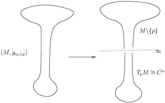
Refer to caption
Figure 4. Explosion of a manifold at pp

Using the Darboux family, for any p∈Mp\in M, we define a 1-parameter family of metrics gε0,ε,pg_{\varepsilon_{0},\varepsilon,p} on MM as the following:

gε0,ε,p={1ε02​gx∈M\Bε0​(p)ρ+​(x)​1ε02​g+(1−ρ+−ρ−)​I∗​(g​(p))(r∘(exppI)−​1)2+ρ−​(x)​1ε2​I∗​(g⁡(p))x∈Bε0​(p)\Bε​(p)1ε2​I∗​(g⁡(p))x∈Bε​(p),g_{\varepsilon_{0},\varepsilon,p}=\left\{\begin{array}[]{lcl}\frac{1}{{\varepsilon_{0}}^{2}}g&x\in&M\backslash B_{\varepsilon_{0}}(p)\\ \rho_{+}(x)\frac{1}{{\varepsilon_{0}}^{2}}g+(1-\rho_{+}-\rho_{-})\frac{I_{*}(g(p))}{(r\circ(\exp_{p}^{I})^{-}1)^{2}}\\ \hskip 36.135pt+\rho_{-}(x)\frac{1}{\varepsilon^{2}}I_{*}(g(p))&x\in&B_{\varepsilon_{0}}(p)\backslash B_{\varepsilon}(p)\\ \frac{1}{\varepsilon^{2}}I_{*}(g(p))&x\in&B_{\varepsilon}(p),\end{array}\right. (8.2)

where the rr is the radius function on (Tp​M,g⁡(p))(T_{p}M,g(p)), the ρ+​(x)\rho_{+}(x) is a smooth cut function that ρ+​(x)=1\rho_{+}(x)=1 outside Bε0​(p)B_{\varepsilon_{0}}(p) and ρ⁡(x)=0\rho(x)=0 in B910​ε0​(p)B_{\frac{9}{10}\varepsilon_{0}}(p), while ρ−​(x)\rho_{-}(x) is another smooth cut function that ρ−​(x)=0\rho_{-}(x)=0 outside B1110​ε​(p)B_{\frac{11}{10}\varepsilon}(p) and ρ⁡(x)=1\rho(x)=1 in Bε​(p)B_{\varepsilon}(p).

We equip M\{p}M\backslash\{p\} with of metric gε0,pg_{\varepsilon_{0},p} making it to be a manifold with one cylindrical end, where

gε0,p={1ε02​gx∈M\Bε0​(p)ρ+​(x)​1ε02​g+(1−ρ+​(x))​I∗​(g​(p))(r∘(exppI)−​1)2x∈Bε0​(p)g_{\varepsilon_{0},p}=\left\{\begin{array}[]{lcl}\frac{1}{{\varepsilon_{0}}^{2}}g&x\in&M\backslash B_{\varepsilon_{0}}(p)\\ \rho_{+}(x)\frac{1}{{\varepsilon_{0}}^{2}}g+(1-\rho_{+}(x))\frac{I_{*}(g(p))}{(r\circ(\exp_{p}^{I})^{-}1)^{2}}&x\in&B_{\varepsilon_{0}}(p)\end{array}\right. (8.3)

We also equip Tp​MT_{p}M with a metric gc​y​l,ε,pg_{cyl,\varepsilon,p} making it to be a manifold with one cylindrical end as well, where

gc​y​l,ε,p={(1−ρ−​(x))​g⁡(p)r2+ρ−​(x)​1ε2​g​(p)x∈Tp​M\Bε​(p)1ε2​g​(p)x∈Bε​(p).g_{cyl,\varepsilon,p}=\left\{\begin{array}[]{lcl}(1-\rho_{-}(x))\frac{g(p)}{r^{2}}+\rho_{-}(x)\frac{1}{\varepsilon^{2}}g(p)&x\in&T_{p}M\backslash B_{\varepsilon}(p)\\ \frac{1}{\varepsilon^{2}}g(p)&x\in&B_{\varepsilon}(p).\end{array}\right. (8.4)

Clearly, the scaling map ε:(Tp​M,gc​y​l,1,p)→(Tp​M,gc​y​l,ε,p)\varepsilon:(T_{p}M,g_{cyl,1,p})\to(T_{p}M,g_{cyl,\varepsilon,p}), v↦v/εv\mapsto v/\varepsilon is an isometry and (Tp​M,gc​y​l,1,p)(T_{p}M,g_{cyl,1,p}) is isometric to (ℂn,gc​y​l,1,0)({\mathbb{C}}^{n},g_{cyl,1,0}).

Remark 8.3.

We have the following observations:

  1. (1)

    The metric gε0,ε,pg_{\varepsilon_{0},\varepsilon,p} on MM is the interpolation of the metrics gε0,pg_{\varepsilon_{0},p} and gc​y​l,ε,pg_{cyl,\varepsilon,p}.

  2. (2)

    limε→0gε0,ε,p=gε0,p\lim_{\varepsilon\to 0}g_{\varepsilon_{0},\varepsilon,p}=g_{\varepsilon_{0},p} on M\{p}M\backslash\{p\}.

  3. (3)

    The expression I∗​(g​(p))(r∘(exppI)−​1)2\frac{I_{*}(g(p))}{(r\circ(\exp_{p}^{I})^{-}1)^{2}} is simply the push-forward of the cylindrical metric gr2=gℝ×S2​n−1\frac{g}{r^{2}}=g_{{\mathbb{R}}\times S^{2n-1}} on Tp​M\{p}T_{p}M\backslash\{p\} to MM by exppI\exp_{p}^{I}.

  4. (4)

    The degenerating metric gε0,ε,pg_{\varepsilon_{0},\varepsilon,p} on MM given is non-collapsing as ε→0\varepsilon\to 0, and

    gε0,p=limε→0gε0,ε,pon​M\{p}.g_{\varepsilon_{0},p}=\lim_{\varepsilon\to 0}g_{\varepsilon_{0},\varepsilon,p}\;\qquad\text{on}\;M\backslash\{p\}.

    in the Gromov-Hausdorff topology.

We note that Bε0​(p)\Bε​(p)B_{\varepsilon_{0}}(p)\backslash B_{\varepsilon}(p) is identified with

(0,ln(ε0)−lnε]×S2​n−1⊂ℝ×S2​n−1(0,\ln(\varepsilon_{0})-\ln\varepsilon]\times S^{2n-1}\subset{\mathbb{R}}\times S^{2n-1}

via the map (r,Θ)↦(s,Θ)(r,\Theta)\mapsto(s,\Theta) with s=ln⁡rs=\ln r. In the coordinates (s,Θ)(s,\Theta), any point x∈Bε0​(p)x\in B_{\varepsilon_{0}}(p) is identified to a pair

(s(x),Θ(x))∈(−∞,0]×S2​n−1.(s(x),\Theta(x))\in(-\infty,0]\times S^{2n-1}.

We call (s,Θ)(s,\Theta) the cylindrical coordinate chart near pp.

Now we equip E⁡(M)×M×ℝ+→M×ℝ+E(M)\times M\times{\mathbb{R}}_{+}\to M\times{\mathbb{R}}_{+} with the structure of Riemannian fibration with its fibers given by

{(M,gε0,ε,p)for ​(p,ε)∈M×ℝ+,ε≠0(Tp​M,g⁡(p))for ​(p,ε)=(p,0)\begin{cases}(M,g_{\varepsilon_{0},\varepsilon,p})\quad&\mbox{for }\,(p,\varepsilon)\in M\times{\mathbb{R}}_{+},\,\varepsilon\neq 0\\ (T_{p}M,g(p))\quad&\mbox{for }\,(p,\varepsilon)=(p,0)\end{cases}

This fibration over ε>0\varepsilon>0 will host the off-shell Banach manifolds for the resolved Floer trajectories arising from nodal Floer trajectories, while the union

E0​#​(M∖{p})=Tp​M​#​(M∖{p})E_{0}\#(M\setminus\{p\})=T_{p}M\#(M\setminus\{p\})

regarded as the end-connected sum of two symplectic manifolds E0E_{0} and M∖{p}M\setminus\{p\}: Here E0E_{0} has convex end and M∖{p}M\setminus\{p\} has concave end both with the unit sphere S1​(Tp​M)S^{1}(T_{p}M) as their asymptotic boundaries in the Darboux chart IpI_{p}. This explosion E⁡(M)×M×ℝ+→M×ℝ+E(M)\times M\times{\mathbb{R}}_{+}\to M\times{\mathbb{R}}_{+} will be implicitly used to define a Banach manifold that host the enhanced nodal Floer trajectories. We turn to the description of these off-shell Banach manifolds in the next couple of subsections.

8.2. Off-shell formulation for perturbed JJ-holomorphic discs

The off-shell formulation of the moduli space ℳ(0,2,0)S​F​T​(ℂn){\mathcal{M}}^{SFT}_{(0;2,0)}({\mathbb{C}}^{n}) has been given in subsection 5.2. Here we provide the off-shell setting for the perturbed JJ-holomorphic disk moduli spaces ℳ⁡((K−,J−),[z−,w−],A−){\mathcal{M}}((K^{-},J^{-});[z_{-},w_{-}];A_{-}) and ℳ⁡((K+,J+),[z+,w+],A+){\mathcal{M}}((K^{+},J^{+});[z_{+},w_{+}];A_{+}). Note that if the target is the compact manifold MM, then the off-shell Banach manifold hosting perturbed JJ-holomorphic curves (or discs) is the standard W1,p​(Σ˙,M)W^{1,p}(\dot{\Sigma},M). That formulation was used in “disk-flow-disk” sections.

However, to resolve enhanced nodal Floer trajectories by the scaled gluing method, we need to blow up every point pp in MM. Therefore the off-shell Banach manifold should incorporate this fact for which we need to consider a family of Banach manifold which forms a (locally trivial) fiber bundle over the target manifold MM.

We first introduce the Banach manifold Wα1,p​(Σ˙,M,p,z+,γ+,τ+)W^{1,p}_{\alpha}(\dot{\Sigma},M;p,z_{+},\gamma_{+},\tau_{+}) for each given (p,,z+,γ+,τ+)(p,,z_{+},\gamma_{+},\tau_{+}). Here α=α⁡(τ)\alpha=\alpha(\tau) stands for the weighting function that

α⁡(τ)={e2​π​δ​|τ|τ≤01τ≥0\alpha(\tau)=\begin{cases}e^{2\pi\delta|\tau|}\quad\tau\leq 0\\ 1\quad\qquad\tau\geq 0\end{cases} (8.5)

The space Wα1,p​(Σ˙,M,p,z+,γ+,τ+)W^{1,p}_{\alpha}(\dot{\Sigma},M;p,z_{+},\gamma_{+},\tau_{+}) consists of elements u:(Σ˙,o+)→(M,p)u:(\dot{\Sigma},o_{+})\to(M,p) satisfying the following:

  1. (1)

    u∈Wl​o​c1,pu\in W^{1,p}_{loc}

  2. (2)

    In the analytical chart of a positive puncture e+∈Σe_{+}\in\Sigma, limτ→+∞u⁡(τ,t)=z+​(t)\lim_{\tau\to+\infty}u(\tau,t)=z_{+}(t) for the periodic orbit z+​(t)z_{+}(t) in MM.

  3. (3)

    For sufficiently large τ\tau, u⁡(τ,t)=expz+​(t)⁡(ξ⁡(τ,t))u(\tau,t)=\exp_{z_{+}(t)}(\xi(\tau,t)), and ξ(τ,t)∈Lp([0,+∞)×S1,z+∗(TM))\xi(\tau,t)\in L^{p}\big([0,+\infty)\times S^{1},z_{+}^{*}(TM)\big)

  4. (4)

    In the analytical chart D+≅(−∞,0]×S1D_{+}\cong(-\infty,0]\times S^{1} of the marked point o+o_{+}, u⁡(τ,t)u(\tau,t) is in a cylindrical coordinate chart Bε0​(p)B_{\varepsilon_{0}}(p) of pp, with u⁡(τ,t)=(Θ+​(τ,t),s+​(τ,t))u(\tau,t)=\big(\Theta_{+}(\tau,t),s_{+}(\tau,t)\big), satisfying

    e2​π​δ​|τ|p∥Θ+(τ,t)−γ+(t)∥S2​n−1∈W1,p((−∞,0]×S1,ℝ)e^{\frac{2\pi\delta|\tau|}{p}}\|\Theta_{+}(\tau,t)-\gamma_{+}(t)\|_{S^{2n-1}}\in W^{1,p}((-\infty,0]\times S^{1},{\mathbb{R}})
    e2​π​δ​|τ|p|s+(τ,t)−2π(τ−τ+)|∈W1,p((−∞,0]×S1,ℝ)e^{\frac{2\pi\delta|\tau|}{p}}|s_{+}(\tau,t)-2\pi(\tau-\tau_{+})|\in W^{1,p}((-\infty,0]\times S^{1},{\mathbb{R}})

    for the simple Reeb orbit γ+​(t)\gamma_{+}(t) and τ+∈ℝ\tau_{+}\in\mathbb{R}.

Wα1,p​(Σ˙,M,p−,z−,γ−,τ−)W^{1,p}_{\alpha}(\dot{\Sigma},M;p_{-},z_{-},\gamma_{-},\tau_{-}) is defined similarly, but the weight function α\alpha is replaced by α⁡(−τ)\alpha(-\tau).

Remark 8.4.

We only consider simple Reeb orbits because we have chosen a generic JJ so that the nodal point p=u−​(o−)=u+​(o+)p=u_{-}(o_{-})=u_{+}(o_{+}) of any nodal Floer trajectory (u−,u+)(u_{-},u_{+}) is immersed. Translating this to the asymptote of u±u_{\pm} in the cylindrical manifold M\{p}M\backslash\{p\}, we only get simple Reeb orbits in S2​n−1S^{2n-1}. Therefore, to host such u±u_{\pm} with immersed at o±o_{\pm}, the function spaces Wα1,p​(Σ˙,M,p±,z±,γ±,τ±)W^{1,p}_{\alpha}(\dot{\Sigma},M;p_{\pm},z_{\pm},\gamma_{\pm},\tau_{\pm}) with simple Reeb orbits γ±\gamma_{\pm} are adequate.

We denote the set of parameterized simple Reeb orbits γ⁡(t)\gamma(t) in S2​n−1S^{2n-1} by ℛ~1​(λ)\widetilde{\mathcal{R}}_{1}(\lambda). By the Hopf fibration S2​n−1→ℂ​PnS^{2n-1}\to{\mathbb{C}}P^{n} we see ℛ~1​(λ)≅S2​n−1\widetilde{\mathcal{R}}_{1}(\lambda)\cong S^{2n-1}, because given any point in S2​n−1S^{2n-1} to start, the passing S1S^{1} fiber is a simple Reeb orbit.

Remark 8.5.

Since there are only finitely many nodal Floer trajectories (u−,u+)(u_{-},u_{+}) during gluing, we can assume the ‖∇u±​(o±)‖\|\nabla u_{\pm}(o_{\pm})\| ( gradient is with respect to the metric gg on MM ) is uniformly bounded. Therefore by possibly shrinking the cylindrical charts O±O_{\pm}, we can assume they all satisfy u±​(O±)⊂Upu_{\pm}(O_{\pm})\subset U_{p}. Therefore, for (τ,t)∈O±(\tau,t)\in O_{\pm}, u±​(τ,t)u_{\pm}(\tau,t) is in the cylindrical coordinate of the target (M\{p},gδ,p)(M\backslash\{p\},g_{\delta,p}) . This said, in cylindrical coordinates of the domain and target,

u±:O±→Bε0(p)≅(−∞,0]×S2​n−1,(τ,t)→(s±(τ,t),Θ±(τ,t))u_{\pm}:O_{\pm}\to B_{\varepsilon_{0}}(p)\cong(-\infty,0]\times S^{2n-1},\;(\tau,t)\to(s_{\pm}(\tau,t),\Theta_{\pm}(\tau,t))

has the asymptote

|∇k(Θ±​(τ,t)−γ±​(t))|S2​n−1\displaystyle|\nabla^{k}(\Theta_{\pm}(\tau,t)-\gamma_{\pm}(t))|_{S^{2n-1}} ≤\displaystyle\leq Ck​e−2​π​ck​|τ|pand\displaystyle C_{k}e^{\frac{-2\pi c_{k}|\tau|}{p}}\qquad\text{and}
|∇k(s±(τ,t)−2​π​(τ−τ±))|\displaystyle|\nabla^{k}(s{\pm}(\tau,t)-2\pi(\tau-\tau_{\pm}))| ≤\displaystyle\leq Ck​e−2​π​ck​|τ|p\displaystyle C_{k}e^{\frac{-2\pi c_{k}|\tau|}{p}} (8.6)

for some constant CkC_{k} and ckc_{k}, where s±=s∘u±s_{\pm}=s\circ u_{\pm} and Θ±=Θ∘u±\Theta_{\pm}=\Theta\circ u_{\pm}. The CkC_{k} and ckc_{k} can be made uniform for all u±u_{\pm} nearby the (finitely many) nodal Floer trajectories (u−,u+)(u_{-},u_{+}) by the continuity of the ∇k+1u±\nabla^{k+1}u_{\pm} translated into cylindrical coordinate. We chose δ\delta in the definition of Wα1,p​(Σ˙,M,p±,z±,γ±,τ±)W^{1,p}_{\alpha}(\dot{\Sigma},M;p_{\pm},z_{\pm},\gamma_{\pm},\tau_{\pm}) to be less than ck​(k=0,1,2)c_{k}(k=0,1,2).

Then we let

Wα1,p​(Σ˙,M,z+):=⋃p∈M⋃(γ+,τ+)∈ℛ~1​(λ)×ℝWα1,p​(Σ˙,M,p,z+,γ+,τ+),W^{1,p}_{\alpha}(\dot{\Sigma},M;z_{+}):=\bigcup_{p\in M}\bigcup_{(\gamma_{+},\tau_{+})\in\widetilde{{\mathcal{R}}}_{1}(\lambda)\times{\mathbb{R}}}W^{1,p}_{\alpha}(\dot{\Sigma},M,p,z_{+},\gamma_{+},\tau_{+}),

where ℛ~1​(λ)\widetilde{{\mathcal{R}}}_{1}(\lambda) is the set of all parameterized simple Reeb orbits in S2​n−1S^{2n-1}. So 𝒲α1,p​(Σ˙,M,z+)\mathcal{W}^{1,p}_{\alpha}(\dot{\Sigma},M;z_{+}) is the space that hosts all (K−,J−)(K_{-},J_{-})-holomorphic discs u+u_{+} with boundary on the periodic orbit z+​(t)z_{+}(t) in MM, and immersion at o+o_{+}. The moduli space Wα1,p​(Σ˙,M,z−)W^{1,p}_{\alpha}(\dot{\Sigma},M;z_{-}) is defined similarly.

We will show Wα1,p​(Σ˙,M,z+)W^{1,p}_{\alpha}(\dot{\Sigma},M;z_{+}) is a Banach manifold. First we describe the tangent space of a given element uu in Wα1,p​(Σ˙,M,z+)W^{1,p}_{\alpha}(\dot{\Sigma},M;z_{+}). Since

π:Wα1,p​(Σ˙,M,z+)→M\pi:W^{1,p}_{\alpha}(\dot{\Sigma},M;z_{+})\to M

is a fiber bundle with its fiber at p∈Mp\in M given by

Wα1,p​(Σ˙,M,p,z+):=⋃(γ+,τ+)∈ℛ~1​(λ)×ℝWα1,p​(Σ˙,M,p,z+,γ+,τ+)W^{1,p}_{\alpha}(\dot{\Sigma},M,p,z_{+}):=\bigcup_{(\gamma_{+},\tau_{+})\in\widetilde{{\mathcal{R}}}_{1}(\lambda)\times{\mathbb{R}}}W^{1,p}_{\alpha}(\dot{\Sigma},M,p,z_{+},\gamma_{+},\tau_{+})

we need to consider both the vertical and horizontal variations for uu.

Let χ+:(−∞,0]→[0,1]\chi_{+}:(-\infty,0]\to[0,1] be a smooth function such that χ+​(τ)=1\chi_{+}(\tau)=1 for τ≤−2\tau\leq-2 and χ+​(τ)=0\chi_{+}(\tau)=0 for τ≥−1\tau\geq-1. We consider the quadruple (U,Vℛ~1​(λ)+,Vℝ+,v+)(U,V^{+}_{\widetilde{{\mathcal{R}}}_{1}(\lambda)},V^{+}_{\mathbb{R}},v_{+}) satisfying

  1. (1)

    Vℛ~1​(λ)+∈Tγ+​ℛ~1​(λ)V^{+}_{\widetilde{{\mathcal{R}}}_{1}(\lambda)}\in T_{\gamma_{+}}\widetilde{{\mathcal{R}}}_{1}(\lambda), Vℝ+∈ℝ=Tτ+​ℝV^{+}_{\mathbb{R}}\in\mathbb{R}=T_{\tau_{+}}\mathbb{R}, and v+∈Tp​Mv_{+}\in T_{p}M, where p=u⁡(o+);p=u(o_{+});

  2. (2)

    U∈Wl​o​c1,p​((Σ˙,u∗​T​M)CLOSE;U\in W^{1,p}_{loc}((\dot{\Sigma},u^{*}TM);

  3. (3)

    U∈Wδ1,p([0,+∞)×S1,u∗TM)U\in W_{\delta}^{1,p}([0,+\infty)\times S^{1},u^{*}TM), where [0,+∞)×S1[0,+\infty)\times S^{1} is the analytical chart for the positive puncture e+∈Σe_{+}\in\Sigma;

  4. (4)

    In the analytical chart D+≅(−∞,0]×S1D_{+}\cong(-\infty,0]\times S^{1} of the marked point o+o_{+}, u⁡(τ,t)u(\tau,t) is in the cylindrical chart of p∈Mp\in M. Let

    U~​(τ,t)\displaystyle\widetilde{U}(\tau,t) =\displaystyle= U⁡(τ,t)−χ+​(τ)​P​a​lu⁡(τ,t)​U​(−∞,t),\displaystyle U(\tau,t)-\chi_{+}(\tau)Pal_{u(\tau,t)}U(-\infty,t),

    then e2​π​δ​|τ|p​|U~​(τ,t)|∈W1,p​((−∞,0)×S1,ℝ)e^{\frac{2\pi\delta|\tau|}{p}}|\widetilde{U}(\tau,t)|\in W^{1,p}((-\infty,0)\times S^{1},{\mathbb{R}}). Here U⁡(−∞,t)=Vℛ~1​(λ)+​(t)U(-\infty,t)=V^{+}_{\widetilde{{\mathcal{R}}}_{1}(\lambda)}(t), and P​a​lu⁡(τ,t)​U​(−∞,t)Pal_{u(\tau,t)}U(-\infty,t) is the parallel transport of U⁡(−∞,t)U(-\infty,t) from u⁡(−∞,t)u(-\infty,t) to u⁡(τ,t)u(\tau,t) along the minimal geodesic in (M,gε0,p)(M,g_{\varepsilon_{0},p}).

Let C0​(u)C^{0}(u) be the set of all such quadruples. It becomes a Banach space with the norm

‖(U,Vℛ~1​(λ)+,Vℝ+,v+)‖1,p,αp=‖e2​π​δ​|τ|p​U~​(τ,t)‖W1,pp+|Vℝ+|p+|Vℛ~1​(λ)+|p+|v+|p.\|(U,V_{\widetilde{{\mathcal{R}}}_{1}(\lambda)}^{+},V_{{\mathbb{R}}}^{+},v_{+})\|^{p}_{1,p,\alpha}=\left\|e^{\frac{2\pi\delta|\tau|}{p}}\widetilde{U}(\tau,t)\right\|^{p}_{W^{1,p}}{}+|V_{{\mathbb{R}}}^{+}|^{p}+|V_{\widetilde{{\mathcal{R}}}_{1}(\lambda)}^{+}|^{p}+|v_{+}|^{p}. (8.7)

Then it is standard to check Wα1,p​(Σ˙,M,z+)W^{1,p}_{\alpha}(\dot{\Sigma},M;z_{+}) is a Banach manifold and

C0​(u)=Tu​Wα1,p​(Σ˙,M,z+).C^{0}(u)=T_{u}W^{1,p}_{\alpha}(\dot{\Sigma},M;z_{+}).

Similarly Wα1,p​(Σ˙,M,z−)W^{1,p}_{\alpha}(\dot{\Sigma},M;z_{-}) is a Banach manifold. The tangent vector

(U,Vℛ~1​(λ)−,Vℝ−,v−)∈Tu​Wα1,p​(Σ˙,M,z−)(U,V_{\widetilde{{\mathcal{R}}}_{1}(\lambda)}^{-},V_{{\mathbb{R}}}^{-},v_{-})\in T_{u}W^{1,p}_{\alpha}(\dot{\Sigma},M;z_{-})

is defined similarly, where Vℛ~1​(λ)−∈Tγ−​ℛ~1​(λ)V_{\widetilde{{\mathcal{R}}}_{1}(\lambda)}^{-}\in T_{\gamma_{-}}\widetilde{{\mathcal{R}}}_{1}(\lambda), Vℝ−∈ℝ=Tτ−​ℝV^{-}_{\mathbb{R}}\in\mathbb{R}=T_{\tau_{-}}\mathbb{R}, and v−∈Tp​Mv_{-}\in T_{p}M, p=u⁡(o−)p=u(o_{-}). The Banach norm is

‖(U,Vℛ~1​(λ)−,Vℝ−,v−)‖1,p,αp=‖e2​π​δ​|τ|p​U~​(τ,t)‖W1,pp−|Vℝ+|p+|Vℛ~1​(λ)−|p+|v−|p.\|(U,V_{\widetilde{{\mathcal{R}}}_{1}(\lambda)}^{-},V_{{\mathbb{R}}}^{-},v_{-})\|^{p}_{1,p,\alpha}=\left\|e^{\frac{2\pi\delta|\tau|}{p}}\widetilde{U}(\tau,t)\right\|^{p}_{W^{1,p}}{}-|V_{{\mathbb{R}}}^{+}|^{p}+|V_{\widetilde{{\mathcal{R}}}_{1}(\lambda)}^{-}|^{p}+|v_{-}|^{p}. (8.8)
Remark 8.6.

UU corresponds to the variation of uu within a fixed fiber M\{p}M\backslash\{p\}, and v+∈Tp​Mv_{+}\in T_{p}M corresponds to the variation of the fiber M\{p}M\backslash\{p\} in M~\widetilde{M}.

Let

ℬ+=Wα1,p(Σ˙,M;z+),ℒ+=⋃u∈ℬ+Lαp(Σ˙,ΛJ+0,1(u+∗(TM))),and\displaystyle\mathcal{B}_{+}=W^{1,p}_{\alpha}(\dot{\Sigma},M;z_{+}),\qquad\mathcal{L}_{+}=\bigcup_{u\in\mathcal{B}_{+}}L^{p}_{\alpha}(\dot{\Sigma},\Lambda^{0,1}_{J^{+}}(u_{+}^{*}(TM))),\quad\text{and}
∂¯(J+,K+):ℬ+→ℒ+,(u,p)→(∂¯J+​u+(PK+)J+(0,1)​(u),p).\displaystyle\overline{\partial}_{(J^{+},K^{+})}:\mathcal{B}_{+}\to\mathcal{L}_{+},\quad(u,p)\to({\overline{\partial}}_{J^{+}}u+(P_{K^{+}})_{J^{+}}^{(0,1)}(u),p).

Then ∂¯(J+,K+)\overline{\partial}_{(J^{+},K^{+})} is a section of the Banach bundle ℬ+→ℒ+\mathcal{B}_{+}\to\mathcal{L}_{+}, and the perturbed (J+,K+)(J^{+},K^{+})-holomorphic disk moduli space ℳ⁡(J+,K+,z+){\mathcal{M}}(J^{+},K^{+};z_{+}) can be written as the zero set

ℳ1​(J+,K+,z+)=(∂¯(J+,K+))−1​(0).{\mathcal{M}}_{1}(J^{+},K^{+};z_{+})=(\overline{\partial}_{(J^{+},K^{+})})^{-1}(0).

When we consider the moduli space with more topological restrictions on uu, say ℳ1​(K+,J+,[z+,w+],A+){\mathcal{M}}_{1}(K^{+},J^{+};[z_{+},w_{+}];A_{+}), we can accordingly restrict to

∂¯(J+,K+):ℬ+​([z+,w+],A+)→ℒ+​([z+,w+],A+),{\overline{\partial}}_{(J^{+},K^{+})}:{\mathcal{B}}_{+}([z_{+},w_{+}];A_{+})\to{\mathcal{L}}_{+}([z_{+},w_{+}];A_{+}),

and get ℳ1​(K+,J+,[z+,w+],A+)=(∂¯(J+,K+))−1​(0){\mathcal{M}}_{1}(K^{+},J^{+};[z_{+},w_{+}];A_{+})=({\overline{\partial}}_{(J^{+},K^{+})})^{-1}(0). Here

ℬ+​([z+,w+],A+)={u∈ℬ+|[u​#​w+]=A+}{\mathcal{B}}_{+}([z_{+},w_{+}];A_{+})=\{u\in{\mathcal{B}}_{+}|\;[u\#w_{+}]=A_{+}\}

and so ℬ+=ℬ+​(z+){\mathcal{B}}_{+}={\mathcal{B}}_{+}(z_{+}) is decomposed into

ℬ+=⋃A+ℬ+​([z+,w+],A+).{\mathcal{B}}_{+}=\bigcup_{A_{+}}{\mathcal{B}}_{+}([z_{+},w_{+}];A_{+}).

And

ℒ+​([z+,w+],A+)=ℒ+|ℬ+​([z+,w+],A+)→ℬ+​([z+,w+],A+){\mathcal{L}}_{+}([z_{+},w_{+}];A_{+})={\mathcal{L}}_{+}|_{\mathcal{B}_{+}([z_{+},w_{+}];A_{+})}\to{\mathcal{B}}_{+}([z_{+},w_{+}];A_{+})

is the restriction of the bundle ℒ+→ℬ+{\mathcal{L}}_{+}\to{\mathcal{B}}_{+} to ℬ+​([z+,w+],A+){\mathcal{B}}_{+}([z_{+},w_{+}];A_{+}). We also note that ℬ+​([z+,w+],A+){\mathcal{B}}_{+}([z_{+},w_{+}];A_{+}) has the decomposition

ℬ+​([z+,w+],A+)=⋃p∈Mℬ+​([z+,w+],p,A+){\mathcal{B}}_{+}([z_{+},w_{+}];A_{+})=\bigcup_{p\in M}{\mathcal{B}}_{+}([z_{+},w_{+}],p;A_{+})

that is a fiber bundle over MM with its fiber at p∈Mp\in M given by

ℬ+([z+,w+],p;A+)={(u,o+)∣ℬ+([z+,w+];A+),u(o+)=p}.{\mathcal{B}}_{+}([z_{+},w_{+}],p;A_{+})=\{(u,o_{+})\mid{\mathcal{B}}_{+}([z_{+},w_{+}];A_{+}),\,u(o_{+})=p\}.

We now study the linearization of ∂¯(J+,K+){\overline{\partial}}_{(J^{+},K^{+})}. First we describe the tangent space T(u,p)​ℬ+​([z+,w+],A+)T_{(u,p)}{\mathcal{B}}_{+}([z_{+},w_{+}];A_{+}). It decomposes

T(u,p)​ℬ+​([z+,w+],A+)=T(u,p)v​ℬ+​([z+,w+],A+)⊕T(u,p)h​ℬ+​([z+,w+],A+)T_{(u,p)}{\mathcal{B}}_{+}([z_{+},w_{+}];A_{+})=T_{(u,p)}^{v}{\mathcal{B}}_{+}([z_{+},w_{+}];A_{+})\oplus T_{(u,p)}^{h}{\mathcal{B}}_{+}([z_{+},w_{+}];A_{+})

into the vertical and horizontal components for the fibration ℬ+​([z+,w+],A+)→M;(u,p)↦u{\mathcal{B}}_{+}([z_{+},w_{+}];A_{+})\to M;(u,p)\mapsto u. Then we have the canonical identification

T(u,p)v​ℬ+​([z+,w+],A+)=T(u)v​ℬ+​([z+,w+],p,A+)≅Wα1,p​(u∗​T​M,p,z+)T_{(u,p)}^{v}{\mathcal{B}}_{+}([z_{+},w_{+}];A_{+})=T_{(u)}^{v}{\mathcal{B}}_{+}([z_{+},w_{+}],p;A_{+})\cong W^{1,p}_{\alpha}(u^{*}TM;p,z_{+})

where Wα1,p​(u∗​T​M,p,z+)W^{1,p}_{\alpha}(u^{*}TM;p,z_{+}) is the set of (U,Vℛ1​(λ)+,Vℝ+)(U,V^{+}_{{\mathcal{R}}_{1}(\lambda)},V^{+}_{\mathbb{R}}) satisfying the conditions given right above Remark 8.6.

On the other hand, the horizontal space is not canonically given and so we will choose them by prescribing their fiber components in the given trivialization of (E⁡(M)|U≅U×E⁡(M,p)CLOSE(E(M)|_{U}\cong U\times E(M,p). Take a small convex neighborhood UU of pp, and consider the parameterized line γ:[0,1]→U\gamma:[0,1]\to U with γ⁡(0)=p,γ⁡(1)\gamma(0)=p,\,\gamma(1) with constant speed. By the discussion before Proposition 8.2 we have diffeomorphisms φp​γ​(s):(M,{p})→(M,γ⁡(s))\varphi_{p\gamma(s)}:(M,\{p\})\to(M,\gamma(s)). We abbreviate φp​γ​(s)\varphi_{p\gamma(s)} by φs\varphi_{s}. Then the fiber component of the horizontal lifting of v∈Tp​Mv\in T_{p}M at uu in this trivialization is given by

dd​s|s=0​φs∘u=:X0∘u\frac{d}{ds}\Big|_{s=0}\varphi_{s}\circ u=:X_{0}\circ u

where XsX_{s} is the vector field generating the isotopy φs\varphi_{s} to the direction of v=p​p′→v=\vec{pp^{\prime}}. Therefore using the local trivialization of ℬ+​([z+,w+],A+)→M{\mathcal{B}}_{+}([z_{+},w_{+}];A_{+})\to M induced by the family of diffeomorphisms φp​p′\varphi_{pp^{\prime}}, the horizontal lifting of v∈Tp​Mv\in T_{p}M is precisely (X0∘u,v)(X_{0}\circ u,v).

Note that the set of these variations {(X0∘u,v}\{(X_{0}\circ u,v\} defines an a 2​n2n-dimensional subspace of Tu​ℬ+​([z+,w+],A+)T_{u}{\mathcal{B}}_{+}([z_{+},w_{+}];A_{+}) isomorphic to Tp​MT_{p}M. We denote this subspace by T~p​M⊂ℬ+​([z+,w+],A+)\widetilde{T}_{p}M\subset{\mathcal{B}}_{+}([z_{+},w_{+}];A_{+}).

Now we are ready to derive the formula for the linearization. When the variational vector field UU is tangent to a fixed target M\{p}M\backslash\{p\}, the linearization Du​∂¯(J+,K+)​(U)D_{u}{\overline{\partial}}_{(J^{+},K^{+})}(U) at uu is computed in a standard way.

Lemma 8.7.

We have

Du​∂¯(J+,K+)​U∈Lαp​(Σ˙,ΛJ+0,1​(u∗​(T​M))).D_{u}{\overline{\partial}}_{(J^{+},K^{+})}U\in L^{p}_{\alpha}(\dot{\Sigma},\Lambda^{0,1}_{J^{+}}(u^{*}(TM))).
Proof.

In the cylindrical end (−∞,0]×S2​n−1(-\infty,0]\times S^{2n-1} in M\{p}M\backslash\{p\}, the vector field

U−U~=χ+​(τ)​P​a​lu⁡(τ,t)​U​(−∞,t)U-\widetilde{U}=\chi_{+}(\tau)Pal_{u(\tau,t)}U(-\infty,t)

is asymptotically JpJ_{p}-holomorphic: One way to see this is the following: identify (−∞,0]×S2​n−1(-\infty,0]\times S^{2n-1} to ℂn\{0}{\mathbb{C}}^{n}\backslash\{0\} and regard u⁡(τ,t)u(\tau,t) in ℂn\{0}{\mathbb{C}}^{n}\backslash\{0\}. then the push forward of P​a​lu⁡(τ,t)​U​(−∞,t)Pal_{u(\tau,t)}U(-\infty,t) is very close to the vector field

Vℝ+​u​(z)+2​π​e2​π​(τ−τ++−1​t)​Vℛ1​(λ)​(0)V_{{\mathbb{R}}}^{+}u(z)+2\pi e^{2\pi(\tau-\tau_{+}+\sqrt{-1}t)}V_{{\mathcal{R}}_{1}(\lambda)}(0)

in ℂn{\mathbb{C}}^{n} when τ\tau is negative enough. Furthermore we also have limτ→−∞u⁡(τ,t)=p\lim_{\tau\to-\infty}u(\tau,t)=p, and J⁡(u⁡(τ,t))→JpJ(u(\tau,t))\to J_{p}. Therefore we have

|Du​∂¯(J+,K+)​(U−U~)|≤C​e−c​|τ||D_{u}{\overline{\partial}}_{(J^{+},K^{+})}(U-\widetilde{U})|\leq Ce^{-c|\tau|}

and so

U=(U−U~)+U~∈Wα1,p((−∞,0]×S1,ℝ).U=(U-\widetilde{U})+\widetilde{U}\in W^{1,p}_{\alpha}((-\infty,0]\times S^{1},{\mathbb{R}}).

This finishes the proof. ∎

When the variational vector field is induced by a change of base point pp in (M,p)(M,p) in the direction of v∈Tp​Mv\in T_{p}M, it is given by the one whose fiber component of the induced variational vector field at uu is given by X0∘uX_{0}\circ u where XsX_{s} is the vector field generating the isotopy φs\varphi_{s}. We denote by XvX_{v} the X0X_{0} associated to v∈Tp​Mv\in T_{p}M. Of course the component in Tp​MT_{p}M is just vv. Note that the set of these variations {(Xv∘u,v)}\{(X_{v}\circ u,v)\} defines an a 2​n2n-dimensional subspace of T(u,p)​ℬ+​([z+,w+],A+)T_{(u,p)}{\mathcal{B}}_{+}([z_{+},w_{+}];A_{+}) isomorphic to Tp​MT_{p}M. We denote this subspace by Tp​M~⊂T(u,p)​ℬ+​([z+,w+],A+)\widetilde{T_{p}M}\subset T_{(u,p)}{\mathcal{B}}_{+}([z_{+},w_{+}];A_{+}) and (Xv∘u,v):=v~(X_{v}\circ u,v):=\widetilde{v}. With this choice, obviously we have the decomposition

T(u,p)​ℬ+​([z+,w+],A+)\displaystyle T_{(u,p)}{\mathcal{B}}_{+}([z_{+},w_{+}];A_{+}) =\displaystyle= Tu​ℬ+​([z+,w+],p,A+)⊕Tp​M~\displaystyle T_{u}{\mathcal{B}}_{+}([z_{+},w_{+}],p;A_{+})\oplus\widetilde{T_{p}M}
=\displaystyle= Wα1,p​(u∗​T​M,p,z+)⊕Tp​M~.\displaystyle W^{1,p}_{\alpha}(u^{*}TM;p,z_{+})\oplus\widetilde{T_{p}M}.

Now the linearization of the section ∂¯(J+,K+):ℬ+​([z+,w+],A+)→ℒ+​([z+,w+],A+){\overline{\partial}}_{(J^{+},K^{+})}:{\mathcal{B}}_{+}([z_{+},w_{+}];A_{+})\to{\mathcal{L}}_{+}([z_{+},w_{+}];A_{+}) at (u,p)(u,p) along

v~∈Tp​M~⊂T(u,p)​ℬ+​([z+,w+],A+)\widetilde{v}\in\widetilde{T_{p}M}\subset T_{(u,p)}{\mathcal{B}}_{+}([z_{+},w_{+}];A_{+})

is given by (Du​∂¯(J+,K+)​(Xv+∘u),v+)(D_{u}{\overline{\partial}}_{(J^{+},K^{+})}(X_{v_{+}}\circ u),v_{+}) in the above mentioned trivialization of T(u,p)​ℬ+​([z+,w+],A+)T_{(u,p)}{\mathcal{B}}_{+}([z_{+},w_{+}];A_{+}).

A straightforward calculation gives rise to the following

Lemma 8.8.

We have the formula

Du​∂¯(J+,K+)​(Xv+∘u)\displaystyle D_{u}\overline{\partial}_{(J^{+},K^{+})}(X_{v^{+}}\circ u) =\displaystyle= (u∗∇)(0,1)(Xv+∘u)+T(0,1)(du,Xv+∘u)\displaystyle(u^{*}\nabla)^{(0,1)}(X_{v^{+}}\circ u)+T^{(0,1)}(du,X_{v^{+}}\circ u)
+D​PK+​(u)(0,1)​(Xv+∘u)\displaystyle\quad+DP_{K^{+}}(u)^{(0,1)}(X_{v^{+}}\circ u)

where TT is the torsion tensor of the almost complex connection ∇\nabla and the (0,1)(0,1)-parts are taken with respect to J+J^{+}.

Combining all these, we have obtained

Proposition 8.9.

For (u,p)∈ℳ1​(K−,J−,[z+,w+],A+)(u,p)\in{\mathcal{M}}_{1}(K_{-},J_{-};[z_{+},w_{+}];A_{+}),

D(u,p)​∂¯(J+,K+):T(u,p)​Wα1,p​(Σ˙,M,z+)→Lαp​(Σ˙,ΛJ+0,1​(u∗​T​M))⊕Tp​MD_{(u,p)}{\overline{\partial}}_{(J^{+},K^{+})}:T_{(u,p)}W^{1,p}_{\alpha}(\dot{\Sigma},M;z_{+})\to L^{p}_{\alpha}(\dot{\Sigma},\Lambda^{0,1}_{J^{+}}(u^{*}TM))\oplus T_{p}M

is a Fredholm operator with

index⁡Du​∂¯(J+,K+)=n−μ⁡([z+,w+])+2​c1​(A+)\operatorname{index}D_{u}{\overline{\partial}}_{(J^{+},K^{+})}=n-\mu([z_{+},w_{+}])+2c_{1}(A_{+})

Next we prove the following transversality result of the section ∂¯(J+,K+){\overline{\partial}}_{(J^{+},K^{+})}.

Proposition 8.10.

For generic J+∈𝒥ω​MJ^{+}\in{\mathcal{J}}_{\omega}M and any (J+,K+)(J^{+},K^{+})-holomorphic curve uu,

D(u,p)​∂¯(J+,K+):T(u,p)​Wα1,p​(Σ˙,M,z+)→Lαp​(Σ˙,ΛJ+0,1​(u∗​T​M))⊕T​MD_{(u,p)}{\overline{\partial}}_{(J^{+},K^{+})}:T_{(u,p)}W^{1,p}_{\alpha}(\dot{\Sigma},M;z_{+})\to L^{p}_{\alpha}(\dot{\Sigma},\Lambda^{0,1}_{J^{+}}(u^{*}TM))\oplus TM

is surjective.

Proof.

We first consider M\{p}M\backslash\{p\} for a fixed pp, and a fixed asymptote (γ+,τ+)(\gamma_{+},\tau_{+}) in the cylindrical metric on M∖{p}M\setminus\{p\} near the point pp. For the linearization of

∂¯(⋅,K+)\displaystyle{\overline{\partial}}_{(\cdot,K^{+})} :\displaystyle: Wα1,p​(Σ˙,M,p,z+,γ+,τ+)×𝒥ω⟶\displaystyle W^{1,p}_{\alpha}(\dot{\Sigma},M;p,z_{+},\gamma_{+},\tau_{+})\times{\mathcal{J}}_{\omega}\longrightarrow
⋃u∈Wα1,p​(Σ˙,M,p,z+,γ+,τ+)⋃J+∈𝒥ωLαp​(Σ˙,ΛJ+0,1​(u∗​T​M)),\displaystyle\quad\bigcup_{u\in W^{1,p}_{\alpha}(\dot{\Sigma},M;p,z_{+},\gamma_{+},\tau_{+})}\bigcup_{J^{+}\in{\mathcal{J}}_{\omega}}L^{p}_{\alpha}(\dot{\Sigma},\Lambda^{0,1}_{J^{+}}(u^{*}TM)),

standard argument shows that the map

Du​∂¯(⋅,K+):T(u,J+)​(Wα1,p​(Σ˙,M,p,z+,γ+,τ+)×𝒥ω)→Lαp​(Σ˙,ΛJ+0,1​(u∗​T​M))D_{u}{\overline{\partial}}_{(\cdot,K^{+})}:T_{(u,J^{+})}(W^{1,p}_{\alpha}(\dot{\Sigma},M;p,z_{+},\gamma_{+},\tau_{+})\times{\mathcal{J}}_{\omega})\to L^{p}_{\alpha}(\dot{\Sigma},\Lambda^{0,1}_{J^{+}}(u^{*}TM)) (8.9)

is surjective for any given (J+,K+)(J^{+},K^{+})-holomorphic curve u∈Wα1,p​(Σ˙,M,p,z+,γ+,τ+)u\in W^{1,p}_{\alpha}(\dot{\Sigma},M;p,z_{+},\gamma_{+},\tau_{+}).

Now we enlarge the domain of ∂¯(⋅,K+){\overline{\partial}}_{(\cdot,K^{+})} from Wα1,p​(Σ˙,M,p,z+,γ+,τ+)×𝒥ωW^{1,p}_{\alpha}(\dot{\Sigma},M;p,z_{+},\gamma_{+},\tau_{+})\times{\mathcal{J}}_{\omega} to Wα1,p​(Σ˙,M,z+)×𝒥ωW^{1,p}_{\alpha}(\dot{\Sigma},M;z_{+})\times{\mathcal{J}}_{\omega}, i.e.

∂¯(⋅,K+):Wα1,p​(Σ˙,M,z+)×𝒥ω→(⋃u∈Wα1,p​(Σ˙,M,z+)⋃J+∈𝒥ωLαp​(Σ˙,ΛJ+0,1​(u∗​T​M)))⊕T​M.{\overline{\partial}}_{(\cdot,K^{+})}:W^{1,p}_{\alpha}(\dot{\Sigma},M;z_{+})\times{\mathcal{J}}_{\omega}\to\left(\bigcup_{u\in W^{1,p}_{\alpha}(\dot{\Sigma},M;z_{+})}\bigcup_{J^{+}\in{\mathcal{J}}_{\omega}}L^{p}_{\alpha}(\dot{\Sigma},\Lambda^{0,1}_{J^{+}}(u^{*}TM))\right)\oplus TM.

Then for any given (J+,K+)(J^{+},K^{+})-holomorphic curve u∈Wα1,p​(Σ˙,M,z+)u\in W^{1,p}_{\alpha}(\dot{\Sigma},M;z_{+}),

Du∂¯(⋅,K+):T(u,J+)(Wα1,p(Σ˙,M;z+)×𝒥ω)→Lαp(Σ˙,ΛJ+0,1(u∗TM))⊕TMD_{u}{\overline{\partial}}_{(\cdot,K^{+})}:T_{(u_{,}J^{+})}(W^{1,p}_{\alpha}(\dot{\Sigma},M;z_{+})\times{\mathcal{J}}_{\omega})\to L^{p}_{\alpha}(\dot{\Sigma},\Lambda^{0,1}_{J^{+}}(u^{*}TM))\oplus TM

is surjective because (8.9) is surjective.

Now we consider the projection p: Wα1,p​(Σ˙,M,z+)×𝒥ω→𝒥ωW^{1,p}_{\alpha}(\dot{\Sigma},M;z_{+})\times{\mathcal{J}}_{\omega}\to{\mathcal{J}}_{\omega}. Then by Sard-Smale theorem, for any generic J+∈𝒥ωJ^{+}\in{\mathcal{J}}_{\omega}, specifying to J+J_{+} for the above parameterized family of maps Du​∂¯(⋅,K+)D_{u}{\overline{\partial}}_{(\cdot,K^{+})},

Du​∂¯(J+,K+):Tu​Wα1,p​(Σ˙,M,z+)→Lαp​(Σ˙,ΛJ+0,1​(u∗​T​M))⊕T​MD_{u}{\overline{\partial}}_{(J^{+},K^{+})}:T_{u}W^{1,p}_{\alpha}(\dot{\Sigma},M;z_{+})\to L^{p}_{\alpha}(\dot{\Sigma},\Lambda^{0,1}_{J^{+}}(u^{*}TM))\oplus TM

is surjective. ∎

To prepare for the next subsection, we define the 1-jet evaluation map for (u,o+)∈ℳ1​([z+,w+],A+)(u,o_{+})\in{\mathcal{M}}_{1}([z_{+},w_{+}];A_{+}). Recall that in the cylindrical coordinate chart near p=u+​(o+)p=u_{+}(o_{+}), we use the embedding

1δ​(expxI)−1:Bε0​(p)\{p}→(Tp​M,Jp)\{p}≅(ℂn,J0)\{0}≅ℝ×S2​n−1\frac{1}{\delta}(\exp_{x}^{I})^{-1}:B_{\varepsilon_{0}}(p)\backslash\{p\}\to(T_{p}M,J_{p})\backslash\{p\}\cong({\mathbb{C}}^{n},J_{0})\backslash\{0\}\cong{\mathbb{R}}\times S^{2n-1}

to express u=(s,Θ)⊂ℝ×S2​n−1u=(s,\Theta)\subset{\mathbb{R}}\times S^{2n-1} with the asymptotes Θ⁡(τ,t)→γ+​(t)\Theta(\tau,t)\to\gamma_{+}(t) and s⁡(τ,t)→2​π​(τ−τ+)s(\tau,t)\to 2\pi(\tau-\tau_{+}). We define the tangential evaluation map

e​v+#:Wα1,p​(Σ˙,M,z+)→ℝ×ℛ1​(λ),u→(τ+,γ+).ev_{+}^{\#}:W^{1,p}_{\alpha}(\dot{\Sigma},M;z_{+})\to{\mathbb{R}}\times{\mathcal{R}}_{1}(\lambda),\quad u\to(\tau_{+},\gamma_{+}).

All the discussion above in this section hold for ℳ1​(K−,J−,[z−,w−],A−){\mathcal{M}}_{1}(K^{-},J^{-};[z_{-},w_{-}];A_{-}) and Wα1,p​(Σ˙,M,z−)W^{1,p}_{\alpha}(\dot{\Sigma},M;z_{-}) without change of proofs.

Here the α=α⁡(τ)\alpha=\alpha(\tau) is a similar (but different) weighting function as before:

α⁡(τ)={1τ≤0e2​π​|τ|τ≥0\alpha(\tau)=\begin{cases}1\qquad\quad\tau\leq 0\\ e^{2\pi|\tau|}\quad\tau\geq 0\end{cases} (8.10)

We abuse the notation α\alpha and the norm ∥⋅∥1,p,α\|\cdot\|_{1,p,\alpha} for u−u_{-} and u+u_{+}.

The tangential evaluation map of u∈Wδ1,p​(Σ˙,M~,z−)u\in W^{1,p}_{\delta}(\dot{\Sigma},\widetilde{M};z_{-}) is defined similarly up to the sign of τ−\tau_{-}:

e​v−#:Wδ1,p​(Σ˙,M,z−)→ℝ×ℛ1​(λ),u→(τ−,γ−).ev_{-}^{\#}:W^{1,p}_{\delta}(\dot{\Sigma},M;z_{-})\to{\mathbb{R}}\times{\mathcal{R}}_{1}(\lambda),\quad u\to(\tau_{-},\gamma_{-}).

8.3. Off-shell formulation of enhanced nodal Floer trajectories

Now we are ready to define the Banach manifold hosting the enhanced nodal Floer trajectories. For notation brevity, we have set Tx​M\{0}=Tx+​MT_{x}M\backslash\{0\}=T_{x}^{+}M and T​M\oM=T+​MTM\backslash o_{M}=T^{+}M, where oMo_{M} is the zero section of T​MTM. For all xx in MM, identifying each (Tx​M,Jx)(T_{x}M,J_{x}) to (ℂn,J0)({\mathbb{C}}^{n},J_{0}), we get a family of inhomogeneous local models

ℳ(0,2,0)+​(Σ˙,Tx​M)≅ℳ(0,2,0)​(Σ˙,Tx​M)⊕Tx+​M,{\mathcal{M}}_{(0;2,0)}^{+}(\dot{\Sigma},T_{x}M)\cong{\mathcal{M}}_{(0;2,0)}(\dot{\Sigma},T_{x}M)\oplus T_{x}^{+}M, (8.11)

and the corresponding Banach manifolds hosting them

ℬx:=Wδ,(0,2,0)1,p​(Σ˙,Tx​M)⊕Tx+​M,\mathcal{B}_{x}:=W^{1,p}_{\delta,(0;2,0)}(\dot{\Sigma},T_{x}M)\oplus T_{x}^{+}M, (8.12)

and the Banach bundles

ℒx:=⋃u∈ℬxLδp​(Σ˙,Λ0,1​(u∗​T​(Tx​M))CLOSE.\mathcal{L}_{x}:=\bigcup_{u\in\mathcal{B}_{x}}L^{p}_{\delta}(\dot{\Sigma},\Lambda^{0,1}(u^{*}T(T_{x}M)). (8.13)

We emphasize that in defining Wδ,(0,2,0)1,p​(Σ˙,Tx​M)W^{1,p}_{\delta,(0;2,0)}(\dot{\Sigma},T_{x}M), the metric hh in the linear space Tx​MT_{x}M is cylindrical, like the one we defined in ℂn{\mathbb{C}}^{n} in section 6: we let h⁡(z)=λ⁡(z)​g​(x)h(z)=\lambda(z)g(x), where g⁡(x)g(x) is the original Riemannian metric on Tx​MT_{x}M, λ:Tp​M→ℝ+\lambda:T_{p}M\to{\mathbb{R}}_{+} is the same radial function as in 6, such that λ⁡(z)=1|z|g2\lambda(z)=\frac{1}{|z|_{g}^{2}} when |z|g|z|_{g} is sufficiently large.

Refer to caption
Figure 5. The enhanced nodal Floer trajectory

The union of these Banach manifolds, which hosts all local models in different Tx​MT_{x}M, is

ℬl​m​d=⋃x∈Mℬx:=⋃x∈MWδ,(1,2,0)1,p​(Σ˙,Tx​M)⊕Tx+​M{\mathcal{B}}_{lmd}=\bigcup_{x\in M}{\mathcal{B}}_{x}:=\bigcup_{x\in M}W^{1,p}_{\delta,(1;2,0)}(\dot{\Sigma},T_{x}M)\oplus T^{+}_{x}M (8.14)

and the corresponding Banach bundle is

ℒl​m​d=⋃x∈Mℒx.\mathcal{L}_{lmd}=\bigcup_{x\in M}\mathcal{L}_{x}.

Here Tx+​MT^{+}_{x}M is the summand encoding the vector a→=∇f​(x)\vec{a}=\nabla f(x) which is not a zero vector since we assume that the node of the nodal Floer trajectories occur outside the set of critical points of the back-ground Morse function ff. We also note that the group

Autl​m​d⁡(x):=(Tx​M×(ℝ∖{0}))×ℝ\operatorname{Aut}_{lmd}(x):=(T_{x}M\times({\mathbb{R}}\setminus\{0\}))\times{\mathbb{R}}

acts on Wδ,(1,2,0)1,p​(Σ˙,Tx​M)W^{1,p}_{\delta,(1;2,0)}(\dot{\Sigma},T_{x}M) where the factor Tx​MT_{x}M corresponds to the translations on Tx​MT_{x}M, ℝ∖{0}{\mathbb{R}}\setminus\{0\} corresponds to multiplication by non-zero real constant on Tx​MT_{x}M and the last ℝ{\mathbb{R}}-factor corresponds to the domain τ\tau-translations. This action also induces an action on ℒl​m​d{\mathcal{L}}_{lmd}.

We let

π:⋃x∈Mℳ(0,2,0)+​(Σ˙,Tx​M)→M\pi:\bigcup_{x\in M}{\mathcal{M}}_{(0;2,0)}^{+}(\dot{\Sigma},T_{x}M)\to M (8.15)

be the projection to the base MM, and the symplectic field theory evaluation map

e​vS​F​T=(e​v−S​F​T,e​v+S​F​T):ℳ(0,2,0)+​(Σ˙,Tx​M)→ℛ1​(λ)×ΔMℛ1​(λ),ev^{SFT}=(ev_{-}^{SFT},ev_{+}^{SFT}):{\mathcal{M}}_{(0;2,0)}^{+}(\dot{\Sigma},T_{x}M)\to{\mathcal{R}}_{1}(\lambda)\times_{\Delta_{M}}{\mathcal{R}}_{1}(\lambda),
u0→(γ0−,γ0+),u_{0}\to\big(\gamma_{0-},\gamma_{0+}\big),

where γ0±\gamma_{0\pm} are the asymptotic data of the local model u0u_{0}. Here we use the fiber product ℛ1​(λ)×ΔMℛ1​(λ){\mathcal{R}}_{1}(\lambda)\times_{\Delta_{M}}{\mathcal{R}}_{1}(\lambda) to emphasize that γ−\gamma_{-} and γ+\gamma_{+} lie in the same Tp​MT_{p}M, where p=π⁡(u0)p=\pi(u_{0}). (We recall from subsection 8.1 and the paragraph right therebefore that we have made the identification of (Tp​M,Jp,ωp)(T_{p}M,J_{p},\omega_{p}) and ℂn{\mathbb{C}}^{n} using the Darboux family II.)

We form the Banach manifold hosting enhanced nodal Floer trajectories via the fiber product of

πΘ∘e​v−#×πΘ∘e​vS​F​T×πΘ​e​v+#:ℛ1​(λ)×(ℛ1​(λ)×ΔMℛ1​(λ))×ℛ1​(λ)\pi_{\Theta}\circ ev^{\#}_{-}\times\pi_{\Theta}\circ ev_{SFT}\times\pi_{\Theta}ev^{\#}_{+}:{\mathcal{R}}_{1}(\lambda)\times({\mathcal{R}}_{1}(\lambda)\times_{\Delta_{M}}{\mathcal{R}}_{1}(\lambda))\times{\mathcal{R}}_{1}(\lambda)
(u−,u0,u+)→(πΘ∘e​v−#​(u−),e​vS​F​T​(u0),πΘ∘e​v+#​(u+)):(u_{-},u_{0},u_{+})\to(\pi_{\Theta}\circ ev^{\#}_{-}(u_{-}),ev_{SFT}(u_{0}),\pi_{\Theta}\circ ev^{\#}_{+}(u_{+})):

Let Δℛ1​(λ)⊂ℛ1​(λ)×ℛ1​(λ)\Delta_{{\mathcal{R}}_{1}(\lambda)}\subset{\mathcal{R}}_{1}(\lambda)\times{\mathcal{R}}_{1}(\lambda) be the diagonal. Then we define

ℬn​o​d​a​l\displaystyle{\mathcal{B}}_{nodal} :⁣=\displaystyle:= (πΘ∘e​v−#×e​vS​F​T×πΘ∘e​v+#)−1​(Δℛ1​(λ)×ΔMΔℛ1​(λ))\displaystyle\left(\pi_{\Theta}\circ ev^{\#}_{-}\times ev_{SFT}\times\pi_{\Theta}\circ ev^{\#}_{+}\right)^{-1}(\Delta_{{\mathcal{R}}_{1}(\lambda)}\times_{\Delta_{M}}\Delta_{{\mathcal{R}}_{1}(\lambda)}) (8.16)
=\displaystyle= {(u−,u0,u+)∈ℬ−×ℬl​m​d×ℬ+|u−(o−)=u+(o+),\displaystyle\{(u_{-},u_{0},u_{+})\in{\mathcal{B}}_{-}\times{\mathcal{B}}_{lmd}\times{\mathcal{B}}_{+}|\;u_{-}(o_{-})=u_{+}(o_{+}),
πΘ∘ev−#(u−)=evS​F​T−(u0),πΘ∘ev+#(u+)=evS​F​T+(u0)}\displaystyle\quad\pi_{\Theta}\circ ev^{\#}_{-}(u_{-})=ev_{SFT}^{-}(u_{0}),\pi_{\Theta}\circ ev^{\#}_{+}(u_{+})=ev_{SFT}^{+}(u_{0})\}

to be the Banach manifold. Due to the action of (Tx​M×(ℝ∖{0}))×ℝ(T_{x}M\times({\mathbb{R}}\setminus\{0\}))\times{\mathbb{R}} on ℬl​m​d{\mathcal{B}}_{lmd}, the same group acts on ℬn​o​d​a​l{\mathcal{B}}_{nodal}.

From the matching condition it is clear that for any u=(u−,u0,u+)∈ℬn​o​d​a​lu=(u_{-},u_{0},u_{+})\in{\mathcal{B}}_{nodal}, its tangent space is

Tu​ℬn​o​d​a​l\displaystyle T_{u}{\mathcal{B}}_{nodal} =\displaystyle= {(ξ−,ξ0,ξ+)∈Tu+ℬ+×Tu0ℬl​m​d×Tu−ℬ−|\displaystyle\{(\xi_{-},\xi_{0},\xi_{+})\in T_{u_{+}}{\mathcal{B}}_{+}\times T_{u_{0}}{\mathcal{B}}_{lmd}\times T_{u_{-}}{\mathcal{B}}_{-}| (8.17)
v−=v+=v0=v,Vℛ1​(λ)±=Vℛ1​(λ)0±}.\displaystyle\qquad v_{-}=v_{+}=v_{0}=v,V^{\pm}_{{\mathcal{R}}_{1}(\lambda)}=V^{0\pm}_{{\mathcal{R}}_{1}(\lambda)}\}.

where we have the expressions

ξ±\displaystyle\xi_{\pm} =\displaystyle= (U±,Vℛ1​(λ)±,Vℝ±,v±)∈Tu±​ℬ±\displaystyle(U_{\pm},V^{\pm}_{{\mathcal{R}}_{1}(\lambda)},V^{\pm}_{{\mathbb{R}}},v_{\pm})\in T_{u_{\pm}}{\mathcal{B}}_{\pm}
ξ0\displaystyle\xi_{0} =\displaystyle= (U0,Vℛ1​(λ)0−,Vℝ0−,Vℛ1​(λ)0+,Vℝ0+,v0)∈Tu0​ℬl​m​d,\displaystyle(U_{0},V^{0-}_{{\mathcal{R}}_{1}(\lambda)},V^{0-}_{{\mathbb{R}}},V^{0+}_{{\mathcal{R}}_{1}(\lambda)},V^{0+}_{{\mathbb{R}}},v_{0})\in T_{u_{0}}{\mathcal{B}}_{lmd},

and the v0∈Tp​Mv_{0}\in T_{p}M correspond to the variation of the base point pp.

We have a natural Autl​m​d⁡(x)\operatorname{Aut}_{lmd}(x)-equivariant section

∂¯(J,K,f)\displaystyle{\overline{\partial}}_{(J,K,f)} :\displaystyle: ℬn​o​d​a​l→ℒ−×ℒl​m​d×ℒ+,\displaystyle{\mathcal{B}}_{nodal}\to\mathcal{L}_{-}\times\mathcal{L}_{lmd}\times\mathcal{L}_{+},
(u−,u0,u+,p)→(∂¯(J−,K−)​u−,∂¯(Jp,f)​u0,∂¯(J+,K+)​u+),\displaystyle(u_{-},u_{0},u_{+},p)\to\left({\overline{\partial}}_{(J^{-},K^{-})}u_{-},\;{\overline{\partial}}_{(J_{p},f)}u_{0},\;{\overline{\partial}}_{(J^{+},K^{+})}u_{+}\right),

where p=u±​(o±)p=u_{\pm}(o_{\pm}) is the nodal point, and ∂¯(Jp,f)u0=∂¯Jpu0−∇f(p)dτ+Jp∇f(p)dt{\overline{\partial}}_{(J_{p},f)}u_{0}={\overline{\partial}}_{J_{p}}u_{0}-\nabla f(p)d\tau+J_{p}\nabla f(p)dt.

If we put more topological restrictions on u−u_{-} and u+u_{+}, namely if we let

ℬn​o​d​a​l​([z−,w−],[z+,w+],A−,A+)={(u−,u0,u+)∈ℬn​o​d​a​l|[u±​#​w±]=A±},{\mathcal{B}}_{nodal}([z_{-},w_{-}],[z_{+},w_{+}];A_{-},A_{+})=\{(u_{-},u_{0},u_{+})\in{\mathcal{B}}_{nodal}|\;[u_{\pm}\#w_{\pm}]=A_{\pm}\},

then similarly we have the section

∂¯(J,K,f):ℬn​o​d​a​l​([z−,w−],[z+,w+],A−,A+)⟶\displaystyle{\overline{\partial}}_{(J,K,f)}:{\mathcal{B}}_{nodal}([z_{-},w_{-}],[z_{+},w_{+}];A_{-},A_{+})\longrightarrow
ℒ⁡([z−,w−],A−)×ℒl​m​d×ℒ⁡([z+,w+],A+),\displaystyle\qquad\mathcal{L}{([z_{-},w_{-}];A_{-})}\times\mathcal{L}_{lmd}\times\mathcal{L}{([z_{+},w_{+}];A_{+})}, (8.18)

and the moduli space of enhanced nodal Floer trajectories with the background Morse function ff defined in Subsection 5.1 can be interpreted as

ℳn​o​d​a​l​([z−,w−],[z+,w+],A−,A+,(K,J),(f,J0))=(∂¯(J,K,f))−1​(0){\mathcal{M}}^{nodal}([z_{-},w_{-}],[z_{+},w_{+}];A_{-},A_{+};(K,J),(f,J_{0}))=({\overline{\partial}}_{(J,K,f)})^{-1}(0)

from (8.3).

Proposition 8.11.

For generic J−J^{-} and J+J^{+} in 𝒥ω{\mathcal{J}}_{\omega}, any enhanced nodal Floer trajectory u=(u−,u0,u+)∈ℳn​o​d​a​l​([z−,w−],[z+,w+],A−,A+,(K,J),(f,J0))u=(u_{-},u_{0},u_{+})\in{\mathcal{M}}^{nodal}([z_{-},w_{-}],[z_{+},w_{+}];A_{-},A_{+};(K,J),(f,J_{0})) is regular, in the sense that

D(u,p)​∂¯(J,K,f)\displaystyle D_{(u,p)}{\overline{\partial}}_{(J,K,f)} :\displaystyle: T(u,p)​ℬn​o​d​a​l​([z−,w−],[z+,w+],A−,A+)⟶\displaystyle T_{(u,p)}{\mathcal{B}}_{nodal}([z_{-},w_{-}],[z_{+},w_{+}];A_{-},A_{+})\longrightarrow
ℒ⁡([z−,w−],A−)×ℒl​m​d×ℒ⁡([z+,w+],A+)⊕Tp​M\displaystyle\quad\mathcal{L}([z_{-},w_{-}];A_{-})\times\mathcal{L}_{lmd}\times\mathcal{L}([z_{+},w_{+}];A_{+})\oplus T_{p}M

is surjective. Consequently, there exists a right inverse Qε|ε=0Q^{\varepsilon}|_{\varepsilon=0} for D(u,p)​∂¯(J,K,f)D_{(u,p)}{\overline{\partial}}_{(J,K,f)}:

Qε|ε=0\displaystyle Q^{\varepsilon}|_{\varepsilon=0} :\displaystyle: ℒ⁡([z−,w−],A−)×ℒl​m​d×ℒ⁡([z+,w+],A+)⊕Tp​M⟶\displaystyle\quad\mathcal{L}([z_{-},w_{-}];A_{-})\times\mathcal{L}_{lmd}\times\mathcal{L}([z_{+},w_{+}];A_{+})\oplus T_{p}M\longrightarrow (8.19)
T(u,p)​ℬn​o​d​a​l​([z−,w−],[z+,w+],A−,A+).\displaystyle T_{(u,p)}{\mathcal{B}}_{nodal}([z_{-},w_{-}],[z_{+},w_{+}];A_{-},A_{+}).

Before the proof of the proposition, we state a lemma concerning the linearization of the inhomogeneous local model equation with respect to the variation v~=(0,v)∈T(u0,p)​ℬl​m​d\widetilde{v}=(0,v)\in T_{(u_{0},p)}{\mathcal{B}}_{lmd} which is the horizontal lifting of v∈Tp​Mv\in T_{p}M as constructed before for the curves u±u_{\pm}.

Lemma 8.12.

For any (u0,v)∈ℳ(0,2,0)+​(Σ˙,Tx​M)(u_{0},v)\in{\mathcal{M}}_{(0;2,0)}^{+}(\dot{\Sigma},T_{x}M) satisfying

∂¯(Jp,f)u0=∂¯Ju0−∇f(p)dτ+J∇f(p)dt=0,{\overline{\partial}}_{(J_{p},f)}u_{0}={\overline{\partial}}_{J}u_{0}-\nabla f(p)d\tau+J\nabla f(p)dt=0,

and corresponding to the variation v~=(Xv∘u0,v)\widetilde{v}=(X_{v}\circ u_{0},v) in the trivialization constructed by the family φp​p′\varphi_{pp^{\prime}} with v∈Tp​Mv\in T_{p}M, we have

(D(u0,p)​∂¯(Jp,f)​(v~))v∈ℒl​m​d.(D_{(u_{0},p)}{\overline{\partial}}_{(J_{p},f)}(\widetilde{v}))^{v}\in{\mathcal{L}}_{lmd}.

Consequently, the map

D(u0,p)​∂¯(Jp,f):Tu0​ℬl​m​d→ℒl​m​d⊕Tp​MD_{(u_{0},p)}{\overline{\partial}}_{(J_{p},f)}:T_{u_{0}}{\mathcal{B}}_{lmd}\to\mathcal{L}_{lmd}\oplus T_{p}M

is surjective.

Now we go back to the proof of the Proposition 8.11:

Proof.

Let u=(u+,u0,u−)u=(u_{+},u_{0},u_{-}) be an enhanced nodal Floer trajectory with the nodal point pp. In subsection 8.2, we have proved that for generic J±∈𝒥ωJ^{\pm}\in{\mathcal{J}}_{\omega},

D(u±,p)​∂¯(J±,K±):T(u±,p)​ℬ​([z±,w±],A±)→Lδp​(Σ˙,ΛJ±0,1​(u±∗​(T​M)))⊕Tp​MD_{(u_{\pm},p)}{\overline{\partial}}_{(J^{\pm},K^{\pm})}:T_{(u_{\pm},p)}{\mathcal{B}}([z_{\pm},w_{\pm}];A_{\pm})\to L^{p}_{\delta}(\dot{\Sigma},\Lambda^{0,1}_{J_{\pm}}(u_{\pm}^{*}(TM)))\oplus T_{p}M

is surjective. By Proposition 5.4, for generic J±∈𝒥ωJ^{\pm}\in{\mathcal{J}}_{\omega} we have that

e​v−×e​v+:ℳ1​(J−,K−,[z−,w−],A−)×ℳ1​(J+,K+,[z+,w+],A+),ev_{-}\times ev_{+}:{\mathcal{M}}_{1}(J^{-},K^{-};[z_{-},w_{-}];A_{-})\times{\mathcal{M}}_{1}(J^{+},K^{+};[z_{+},w_{+}];A_{+}), (8.20)
(u−,u+)→(u−​(o−),u+​(o+))(u_{-},u_{+})\to(u_{-}(o_{-}),u_{+}(o_{+}))

is transversal to ΔM⊂M×M\Delta_{M}\subset M\times M. Therefore, for any η±∈Lδp​(Σ˙,ΛJ±0,1​(u±∗​(T​M)))\eta_{\pm}\in L^{p}_{\delta}(\dot{\Sigma},\Lambda^{0,1}_{J_{\pm}}(u_{\pm}^{*}(TM))), there exist ξ±=(U±,Vℛ1​(λ)±,Vℝ±,v±)∈Tu±​ℬ​([z±,w±],A±)\xi_{\pm}=(U_{\pm},V^{\pm}_{{\mathcal{R}}_{1}(\lambda)},V^{\pm}_{{\mathbb{R}}},v_{\pm})\in T_{u_{\pm}}{\mathcal{B}}([z_{\pm},w_{\pm}];A_{\pm}) such that

Du±​∂¯(J±,K±)​ξ±=η±, and v−=v+:=v.D_{u_{\pm}}{\overline{\partial}}_{(J^{\pm},K^{\pm})}\xi_{\pm}=\eta_{\pm},\qquad\text{ and }\quad v_{-}=v_{+}:=v.

Then for any η0∈ΛJp0,1​(u0∗​(T​Tp​M))\eta_{0}\in\Lambda^{0,1}_{J_{p}}(u_{0}^{*}(TT_{p}M)), by the transversality of the local models in ℂn≅Tp​M{\mathbb{C}}^{n}\cong T_{p}M, for u0u_{0} in Tp​MT_{p}M, there exists

ξ0=(U0,Vℛ1​(λ)0−,Vℛ1​(λ)0+)∈Tu0​ℬp\xi_{0}=(U_{0},V^{0-}_{{\mathcal{R}}_{1}(\lambda)},V^{0+}_{{\mathcal{R}}_{1}(\lambda)})\in T_{u_{0}}{\mathcal{B}}_{p}

such that Du0​∂¯(Jp,f)​ξ0=η0D_{u_{0}}{\overline{\partial}}_{(J_{p},f)}\xi_{0}=\eta_{0}. Hence for (ξ0,v0)∈T(u0,v0)​ℬl​m​d(\xi_{0},v_{0})\in T_{(u_{0},v_{0})}{\mathcal{B}}_{lmd} with v0=vv_{0}=v,

Du0​∂¯(Jp,f)​(ξ0,v0)=Du0​∂¯Jp,f​ξ0=η0.D_{u_{0}}{\overline{\partial}}_{(J_{p},f)}(\xi_{0},v_{0})=D_{u_{0}}{\overline{\partial}}_{J_{p},f}\xi_{0}=\eta_{0}.

The proposition immediately follows from the surjectivity of Du±​∂¯(J±,K±)D_{u_{\pm}}{\overline{\partial}}_{(J_{\pm},K_{\pm})}, Du0​∂¯(Jp,f)D_{u_{0}}{\overline{\partial}}_{(J_{p},f)} and the transversality of the evaluation map

πΘ∘e​v−#×πΘ∘e​v+#→ℛ1​(λ)×ℛ1​(λ)\pi_{\Theta}\circ ev_{-}^{\#}\times\pi_{\Theta}\circ ev_{+}^{\#}\to{\mathcal{R}}_{1}(\lambda)\times{\mathcal{R}}_{1}(\lambda)

to the diagonal Δℛ1​(λ)\Delta_{{\mathcal{R}}_{1}(\lambda)}. For any η=(η−,η0,η+)\eta=(\eta_{-},\eta_{0},\eta_{+}), using the above construction we define Qε|ε=0Q^{\varepsilon}|_{\varepsilon=0} is defined to be Qε|ε=0​(η)=(ξ−,ξ0,ξ+,v)Q^{\varepsilon}|_{\varepsilon=0}(\eta)=(\xi_{-},\xi_{0},\xi_{+},v). Then Qε|ε=0Q^{\varepsilon}|_{\varepsilon=0} is a right inverse of D(u,p)​∂¯(J,K,f)D_{(u,p)}{\overline{\partial}}_{(J,K,f)} and the proposition follows. ∎

Remark 8.13.

For the purpose of constructing approximate right inverse later, we define the operators Q−Q_{-}, Q0Q_{0} and Q+Q_{+} by

Q−​η−:=ξ−,Q0​η0:=ξ0,Q+​η+:=ξ+Q_{-}\eta_{-}:=\xi_{-},\quad Q_{0}\eta_{0}:=\xi_{0},\quad Q_{+}\eta_{+}:=\xi_{+}

for the (η−,η0,η+)(\eta_{-},\eta_{0},\eta_{+}) and (ξ−,ξ0,ξ+)(\xi_{-},\xi_{0},\xi_{+}) above.

8.4. Appendix : Explosion

In this appendix, we collect various facts on the so called, explosion construction of manifolds. We verbatim follow the exposition in the smooth context given by Weinstein in section 4 [We2].

Let Y⊂XY\subset X be a submanifold. The explosion of XX along YY, denoted by E⁡(X,Y)E(X,Y), is defined by beginning with the product X×ℝX\times{\mathbb{R}}, removing the “axis” X×{0}X\times\{0\}, and replacing it with the normal bundle N⁡(X,Y)=TY​X/T​YN(X,Y)=T_{Y}X/TY to YY in XX. The differentiable structure on E⁡(X,Y)E(X,Y) is taken to be the usual product structure on X×(ℝ×{0})X\times({\mathbb{R}}\times\{0\}). Charts near X×{0}X\times\{0\} are defined with the aid of local coordinates on XX. A more precise description of local charts near X×{0}X\times\{0\} is in order.

Let XX have dimension nn and YY have dimension kk. We abbreviate the coordinates (x1,⋯,xn)(x_{1},\cdots,x_{n}) on ℝn{\mathbb{R}}^{n} by (y,z)(y,z), where y=(x1,⋅,xk)y=(x_{1},\cdot,x_{k}) and z=(xk+1,⋯,xn)z=(x_{k+1},\cdots,x_{n}). Suppose that Φ\Phi is a submanifold fold chart defined on an open subset U⊂XU\subset X at p∈Y⊂Xp\in Y\subset X, i.e., a chart for the pair (X,Y)(X,Y) defined on an open subset 𝒰{\mathcal{U}} of (ℝn,ℝk)({\mathbb{R}}^{n},{\mathbb{R}}^{k}) which is invariant under the retraction (y,z)↦(y,0)(y,z)\mapsto(y,0). The corresponding chart E⁡(Φ)E(\Phi) for E⁡(X,Y)E(X,Y) is defined on the open subset {(y,z′,ε)∣(y,ε​z′)∈𝒰}\{(y,z^{\prime},\varepsilon)\mid(y,\varepsilon z^{\prime})\in{\mathcal{U}}\} of ℝn+1{\mathbb{R}}^{n+1} by

E⁡(Φ)​(y,z′,ε)=(Φ⁡(y,ε​z′),ε)E(\Phi)(y,z^{\prime},\varepsilon)=(\Phi(y,\varepsilon z^{\prime}),\varepsilon) (8.21)

for ε≠0\varepsilon\neq 0 with E​(Φ)​(y,z′,0)E(\Phi)(y,z^{\prime},0) defined as the projection of the tangent vector T(y,0)​Φ​(0,z′)T_{(y,0)}\Phi(0,z^{\prime}) into the normal bundle N⁡(X,Y)N(X,Y). The following theorem is proved by Weinstein [We2].

Theorem 8.14 (Lemma 4.3, [We2]).

Let f:(X,Y)→(Z,W)f:(X,Y)\to(Z,W) be a smooth mapping. Then it uniquely induces a smooth mapping E⁡(f):E⁡(X,Y)→E⁡(Z,W)E(f):E(X,Y)\to E(Z,W) such that

  1. (1)

    E⁡(f)E(f) extends to the restriction f:X∖Y→Z∖Wf:X\setminus Y\to Z\setminus W,

  2. (2)

    When Φ\Phi and Ψ\Psi are local charts of (X,Y)(X,Y) and (Z,W)(Z,W) respectively and the local representative Ψ−1​f​Φ\Psi^{-1}f\Phi is written as Ψ−1​f​Φ=(g,h):(ℝn,ℝk)→(Rm,ℝℓ)\Psi^{-1}f\Phi=(g,h):({\mathbb{R}}^{n},{\mathbb{R}}^{k})\to(R^{m},{\mathbb{R}}^{\ell}), then the local representation E⁡(g,h)E(g,h) of E⁡(f)E(f) with respect to the charts E⁡(Φ)E(\Phi) and E⁡(Ψ)E(\Psi) is given for ε≠0\varepsilon\neq 0 by the “partial difference quotient”

    E⁡(g,h)​(y,z′,e)=(g⁡(y,ε​z′),(1/ε)​h​(y,ε​z′),ε)E(g,h)(y,z^{\prime},e)=(g(y,\varepsilon z^{\prime}),(1/\varepsilon)h(y,\varepsilon z^{\prime}),\varepsilon)

    and for ε=0\varepsilon=0 by the normal derivative

    E⁡(g,h)​(y,z′,0)=(g⁡(y,0),(∂h/∂z′)​(y,0),0).E(g,h)(y,z^{\prime},0)=(g(y,0),(\partial h/\partial z^{\prime})(y,0),0).

Two immediate consequences are also derived in [We2].

Corollary 8.15 (Theorem 4.4, [We2]).

Assuming to each pair (X,Y)(X,Y) the exploded manifold E⁡(X,Y)E(X,Y) with the differentiable structure described above defines a covariant functor from the category of pairs of manifolds to the category of manifolds over ℝ{\mathbb{R}}.

Corollary 8.16.

The identity map on X×(ℝ∖{0})X\times({\mathbb{R}}\setminus\{0\}) extends to a unique smooth mapping from E⁡(X,Y)E(X,Y) to X×ℝX\times{\mathbb{R}}. The restriction of this mapping to N⁡(X,Y)N(X,Y) is the bundle projection onto Y×{0}Y\times\{0\}.

This corollary defines a canonical smooth projection map E⁡(X,Y)→X×ℝE(X,Y)\to X\times{\mathbb{R}}, which we denote by πE⁡(X,Y)\pi_{E(X,Y)}.

Part II Analysis : Scale-dependent gluing and compactification

9. Smoothing of nodal Floer trajectories I ; to ‘disk-flow-disk’

The disk-flow-disk moduli spaces

ℳp​a​r​a​([z−,w−],f,[z+,w+],A±),ℳε​([z−,w−],f,[z+,w+],A±){\mathcal{M}}^{para}([z_{-},w_{-}];f;[z_{+},w_{+}];A_{\pm}),\quad{\mathcal{M}}^{\varepsilon}([z_{-},w_{-}];f;[z_{+},w_{+}];A_{\pm})

have been defined in section 44. Recall that the moduli space of “disk-flow-disk” elements of flow time ε\varepsilon is

ℳε([z−,w−];f;[z+,w+];A±):={(u−,χ,u+)∣u±∈ℳ(K±,J±;z→±;A±),χ:[0,ε]→M,χ˙−∇f(χ)=0,u−(o−)=χ(0),u+(o+)=χ(ε)}{\mathcal{M}}^{\varepsilon}([z_{-},w_{-}];f;[z_{+},w_{+}];A_{\pm}):=\{(u_{-},\chi,u_{+})\mid u_{\pm}\in{\mathcal{M}}(K^{\pm},J^{\pm};\vec{z}_{\pm};A_{\pm}),\\ \chi:[0,\varepsilon]\to M,\dot{\chi}-\nabla f(\chi)=0,\;u_{-}(o_{-})=\chi(0),\;u_{+}(o_{+})=\chi(\varepsilon)\} (9.1)

We give ℳε​([z−,w−],f,[z+,w+],A±){\mathcal{M}}^{\varepsilon}([z_{-},w_{-}];f;[z_{+},w_{+}];A_{\pm}) another interpretation through evaluation maps. This point of view is more suitable for analyzing the transition from nodal Floer trajectories to “disk-flow-disk” elements. Consider the deformed evaluation map

ϕfε​e​v−×e​v+:ℳ1​([z−,w−],A−)×ℳ1​([z+,w+],A+)→M×M\phi_{f}^{\varepsilon}ev_{-}\times ev_{+}:{\mathcal{M}}_{1}([z_{-},w_{-}];A_{-})\times{\mathcal{M}}_{1}([z_{+},w_{+}];A_{+})\to M\times M (9.2)
(u−,u+)→(ϕfε​u−​(o−),u+​(o+)),(u_{-},u_{+})\to(\phi_{f}^{\varepsilon}u_{-}(o_{-}),u_{+}(o_{+})),

where ϕfε:M→M\phi_{f}^{\varepsilon}:M\to M is the time-ε\varepsilon flow of the Morse function ff. Then it is easy to see

ℳε([z−,w−];f;[z+,w+];A±)={(u−,χ,u+)∣(u−,u+)∈(ϕfεev−×ev+)−1(Δ),χ(τ)=ϕfτu−(o−) for 0≤τ≤ε}{\mathcal{M}}^{\varepsilon}([z_{-},w_{-}];f;[z_{+},w_{+}];A_{\pm})=\{(u_{-},\chi,u_{+})\mid\\ (u_{-},u_{+})\in(\phi_{f}^{\varepsilon}ev_{-}\times ev_{+})^{-1}(\Delta),\;\chi(\tau)=\phi_{f}^{\tau}u_{-}(o_{-})\text{ for }0\leq\tau\leq\varepsilon\} (9.3)

Using the above interpretation, if

ϕfε​e​v−×e​v+​ is transversal to ​Δ⊂M×M\phi_{f}^{\varepsilon}ev_{-}\times ev_{+}\text{ is transversal to }\Delta\subset M\times M (9.4)

and if Du±​∂¯(K±,J±)D_{u_{\pm}}{\overline{\partial}}_{(K_{\pm},J_{\pm})} are surjective, then by the inverse function theorem for (9.2), ℳε​([z−,w−],f,[z+,w+],A±){\mathcal{M}}^{\varepsilon}([z_{-},w_{-}];f;[z_{+},w_{+}];A_{\pm}) is a manifold of dimension

dim⁡ℳε​([z−,w−],f,[z+,w+],A±)\displaystyle\operatorname{dim}{\mathcal{M}}^{\varepsilon}([z_{-},w_{-}];f;[z_{+},w_{+}];A_{\pm})
=\displaystyle= dim⁡ℳ⁡([z−,w−],A−)+dim⁡ℳ⁡([z+,w+],A+)−2​n\displaystyle\operatorname{dim}{\mathcal{M}}([z_{-},w_{-}];A_{-})+\operatorname{dim}{\mathcal{M}}([z_{+},w_{+}];A_{+})-2n
=\displaystyle= (n+μC​Z​([z−,w−])+2​c1​(A−))+(n−μC​Z​([z+,w+])+2​c1​(A+))−2​n\displaystyle(n+\mu_{CZ}([z_{-},w_{-}])+2c_{1}(A_{-}))+(n-\mu_{CZ}([z_{+},w_{+}])+2c_{1}(A_{+}))-2n
=\displaystyle= μC​Z​([z−,w−])−μC​Z​([z+,w+])+2​c1​(A−)+2​c1​(A+),\displaystyle\mu_{CZ}([z_{-},w_{-}])-\mu_{CZ}([z_{+},w_{+}])+2c_{1}(A_{-})+2c_{1}(A_{+}),

if ε>0\varepsilon>0 is sufficiently small.

Assumption: For transversality argument, from now on we assume the critical points of ff do not coincide with the nodal points of nodal Floer trajectories, this can be achieved by a generic ff.

Since we mainly care about the transition from disk-flow-disk elements to resolved nodal Floer trajectories during the PSS cobordism, only the disk-flow-disk elements with short-time flows will be considered. So we fix a sufficiently small ε0>0\varepsilon_{0}>0 which is to be determined later, and consider the “disk-flow-disk” moduli spaces ℳε​([z−,w−],f,[z+,w+],A±){\mathcal{M}}^{\varepsilon}([z_{-},w_{-}];f;[z_{+},w_{+}];A_{\pm}) with 0≤ε≤ε00\leq\varepsilon\leq\varepsilon_{0}. The ε=0\varepsilon=0 case corresponds to the moduli space of nodal Floer trajectories.

Lemma 9.1.

Suppose that the almost complex structures J±J^{\pm} are generically chosen so for any nodal Floer trajectory (u−,u+)(u_{-},u_{+}), Du±​∂¯(K±,J±)D_{u_{\pm}}{\overline{\partial}}_{(K_{\pm},J_{\pm})} are surjective, and u−​(o−)u_{-}(o_{-}) and u+​(o+)u_{+}(o_{+}) are immersed points as in Theorem 1.4. Then there exists ε0>0\varepsilon_{0}>0, such that for any (u−,χ,u+)∈ℳε​([z−,w−],f,[z+,w+],A±)(u_{-},\chi,u_{+})\in{\mathcal{M}}^{\varepsilon}([z_{-},w_{-}];f;[z_{+},w_{+}];A_{\pm}) where ε∈[0,ε0]\varepsilon\in[0,\varepsilon_{0}], the above property is preserved, i.e. Du±​∂¯(K±,J±)D_{u_{\pm}}{\overline{\partial}}_{(K_{\pm},J_{\pm})} are surjective, and u−​(o−)u_{-}(o_{-}) and u+​(o+)u_{+}(o_{+}) are immersed points.

Proof.

We prove that u−​(o−)u_{-}(o_{-}) and u+​(o+)u_{+}(o_{+}) are immersed points. Otherwise, there exist εi→0\varepsilon_{i}\to 0, and (u−i,χi,u+i)∈ℳεi​(K±,J±,[z−,w−],f,[z+,w+],A±)(u_{-}^{i},\chi_{i},u_{+}^{i})\in{\mathcal{M}}^{\varepsilon_{i}}(K^{\pm},J^{\pm};[z_{-},w_{-}],f,[z_{+},w_{+}];A_{\pm}), such that at least one of u−i​(o−)u_{-}^{i}(o_{-}) and u+i​(o+)u_{+}^{i}(o_{+}) is not an immersed point. Passing to a subsequence we may assume, say d​u−i​(o−)du_{-}^{i}(o_{-}), is 00 for any ii. Since the energy of any curves u±iu_{\pm}^{i} is uniformly bounded due to the boundary condition, we can take a subsequence again and get a limiting nodal curve (u−∞,u+∞)(u_{-}^{\infty},u_{+}^{\infty}) by Gromov-compactness. The images of χi\chi_{i} converge to the nodal point. No bubbling can occur on u−∞u_{-}^{\infty} or u+∞u_{+}^{\infty}, because if a bubble occurs on u+∞u_{+}^{\infty} or u+∞u_{+}^{\infty}, then by the semi-positive condition and the genericity of J±J^{\pm}, we can resolve the bubble to get a at least two dimensional family of nodal Floer trajectories, contradicting with the rigidity assumption on nodal Floer trajectories. Therefore, the curves (u−i,u+i)(u_{-}^{i},u_{+}^{i}) converge to (u−∞,u+∞)(u_{-}^{\infty},u_{+}^{\infty}) in C1C^{1} topology. This implies d​u−∞​(o−)=limi→∞d​u−i​(o−)=0du_{-}^{\infty}(o_{-})=\lim_{i\to\infty}du_{-}^{i}(o_{-})=0, contradicting with the immersion condition at the nodal point.

Since u±​(o±)u_{\pm}(o_{\pm}) are immersed points, u±u_{\pm} are somewhere injective. Then the genericity of J±J^{\pm} implies that Du±​∂¯(K±,J±)D_{u_{\pm}}{\overline{\partial}}_{(K_{\pm},J_{\pm})} are surjective. ∎

To complete the PSS cobordism from “disk-flow-disk” configurations to nodal Floer trajectories, we will build a collar neighborhood of ℳ0​([z−,w−],f,[z+,w+],A±){\mathcal{M}}^{0}([z_{-},w_{-}],f,[z_{+},w_{+}];A_{\pm}) in ℳp​a​r​a​([z−,w−],f,[z+,w+],A±){\mathcal{M}}^{para}([z_{-},w_{-}];f;[z_{+},w_{+}];A_{\pm}); More precisely, for some ε0>0\varepsilon_{0}>0, we will construct a differentiable map

G:ℳ0​([z−,w−],f,[z+,w+],A±)×[0,ε0)→ℳp​a​r​a​([z−,w−],f,[z+,w+],A±)G:{\mathcal{M}}^{0}([z_{-},w_{-}],f,[z_{+},w_{+}];A_{\pm})\times[0,\varepsilon_{0})\to{\mathcal{M}}^{para}([z_{-},w_{-}];f;[z_{+},w_{+}];A_{\pm})

such that for each ε∈[0,ε0)\varepsilon\in[0,\varepsilon_{0}),

Gε:=G⁡(⋅,ε):ℳ0​([z−,w−],f,[z+,w+],A±)→ℳε​([z−,w−],f,[z+,w+],A±)G_{\varepsilon}:=G(\cdot,\varepsilon):{\mathcal{M}}^{0}([z_{-},w_{-}],f,[z_{+},w_{+}];A_{\pm})\to{\mathcal{M}}^{\varepsilon}([z_{-},w_{-}];f;[z_{+},w_{+}];A_{\pm})

is a diffeomorphism. This problem is reduced to the following finite dimensional differential topology lemma:

Lemma 9.2.

X,Y,ZX,Y,Z are differentiable manifolds, and only XX may have boundary. XX is compact, ZZ is a differentiable submanifold in YY, and II is an interval containing 00. Let Φ:X×I→Y\Phi:X\times I\to Y be a differentiable map. Denote Φε:=Φ⁡(⋅,ε)\Phi_{\varepsilon}:=\Phi(\cdot,\varepsilon) for ε∈I\varepsilon\in I. If Φ0:X→Y\Phi_{0}:X\to Y is transversal to ZZ with nonempty intersection, and Φ0​(∂X)∩Z=∅\Phi_{0}(\partial X)\cap Z=\emptyset, then

  1. (1)

    There exists ε0>0\varepsilon_{0}>0, such that for any ε∈[0,ε0]\varepsilon\in[0,\varepsilon_{0}], Φε\Phi_{\varepsilon} is transversal to ZZ;

  2. (2)

    Furthermore, there exits a differentiable map G:Φ0−1​(Z)×[0,ε0]→Φ−1​(Z)G:\Phi_{0}^{-1}(Z)\times[0,\varepsilon_{0}]\to\Phi^{-1}(Z), such that for any ε∈[0,ε0]\varepsilon\in[0,\varepsilon_{0}], Gε:=G⁡(⋅,ε)G_{\varepsilon}:=G(\cdot,\varepsilon) gives a diffeomorphism from Φ0−1​(Z)\Phi_{0}^{-1}(Z) to Φε−1​(Z)\Phi_{\varepsilon}^{-1}(Z).

Proof.

Since XX is compact, the compact-open topology in the function space C1​(X,Y)C^{1}(X,Y) coincides with the strong topology CS1​(X,Y)C^{1}_{S}(X,Y) as in [Hir]. Since the set of maps transversal to ZZ in CS1​(X,Y)C^{1}_{S}(X,Y) is open, by the condition of Φ\Phi and Φ0\Phi_{0} we conclude that for ε0\varepsilon_{0} sufficiently small,

 for all ​ε∈[0,ε0],Φε​ is transversal to ​Z.\text{ for all }\varepsilon\in[0,\varepsilon_{0}],\Phi_{\varepsilon}\text{ is transversal to }Z. (9.5)

Since Φε​(X)∩Y≠∅\Phi_{\varepsilon}(X)\cap Y\neq\emptyset, and Φ0​(∂X)∩Y=∅\Phi_{0}(\partial X)\cap Y=\emptyset, the pre-image of all intersections lies in int​(X)\text{int}(X), where int​(X)\text{int}(X) is the interior of XX. Therefore for ε0\varepsilon_{0} sufficiently small, for all ε∈[0,ε0]\varepsilon\in[0,\varepsilon_{0}]

Φε​(X)∩Y≠∅\Phi_{\varepsilon}(X)\cap Y\neq\emptyset (9.6)

by analyzing the local behavior of intersections. We also have Φε​(∂X)∩Y=∅\Phi_{\varepsilon}(\partial X)\cap Y=\emptyset, using the compactness of ∂X\partial X and the continuous dependence of Φε\Phi_{\varepsilon} on ε\varepsilon.

Clearly (9.5) implies Φ:X×[0,ε0]→Y\Phi:X\times[0,\varepsilon_{0}]\to Y is transversal to ZZ. So Φ−1​(Z):=W\Phi^{-1}(Z):=W is a differentiable submanifold in X×[0,ε0]X\times[0,\varepsilon_{0}]. Actually it is in int​(X)×[0,ε0]\text{int}(X)\times[0,\varepsilon_{0}], because Φ⁡(∂X×[0,ε0])∩Z=∅\Phi(\partial X\times[0,\varepsilon_{0}])\cap Z=\emptyset. So ∂W⊂X×{0,ε0}\partial W\subset X\times\{0,\varepsilon_{0}\}.

Note the following elementary fact during the proof of parameterized transversality in [Hir]:

Φε​ transversal to ​Y⟺ε​ is a regular value of ​π:W→I,\Phi_{\varepsilon}\text{ transversal to }Y\Longleftrightarrow\varepsilon\text{ is a regular value of }\pi:W\to I, (9.7)

where π:X×I→I\pi:X\times I\to I is the natural projection. Then we have a submersion π:W→[0,ε0]\pi:W\to[0,\varepsilon_{0}] by translating (9.5) via (9.7). By (9.6) π\pi is surjective. Picking any metric on WW, then the gradient vector field ∇π\nabla\pi never vanishes on WW. Let the time-τ\tau flow of the gradient vector field to be φπτ\varphi^{\tau}_{\pi}. By Morse theory we have the diffeomorphism φπε:π−1​(0)→π−1​(ε)\varphi^{\varepsilon}_{\pi}:\pi^{-1}(0)\to\pi^{-1}(\varepsilon) for all ε∈[0,ε0]\varepsilon\in[0,\varepsilon_{0}], using that ∂W⊂X×{0,ε0}\partial W\subset X\times\{0,\varepsilon_{0}\}. Noting that π−1​(ε)=Φε−1​(Z)\pi^{-1}(\varepsilon)=\Phi_{\varepsilon}^{-1}(Z), the map G:=φπ(⋅):Φ0−1​(Z)×[0,ε0]→Φ−1​(Z)G:=\varphi^{(\cdot)}_{\pi}:\Phi_{0}^{-1}(Z)\times[0,\varepsilon_{0}]\to\Phi^{-1}(Z) is desired. ∎

First we derive

Corollary 9.3.

For given generic ff and JJ, there exists a constant ε0>0\varepsilon_{0}>0, such that for all (u−,χ,u+)∈ℳε​([z−,w−],f,[z+,w+],A±)(u_{-},\chi,u_{+})\in{\mathcal{M}}^{\varepsilon}([z_{-},w_{-}];f;[z_{+},w_{+}];A_{\pm}) where ε∈(0,ε0]\varepsilon\in(0,\varepsilon_{0}], the linearized operator E⁡(u)E(u) in Section 5.1 is surjective.

Proof.

In the above lemma, take X=ℳ¯1​([z−,w−],A−)×ℳ¯1​([z+,w+],A+)X=\overline{{\mathcal{M}}}_{1}([z_{-},w_{-}];A_{-})\times\overline{{\mathcal{M}}}_{1}([z_{+},w_{+}];A_{+}), Y=M×MY=M\times M, Z=ΔZ=\Delta and Φ:X×I→Y\Phi:X\times I\to Y to be

ϕfε​e​v−×e​v+:ℳ⁡([z−,w−],A−)×ℳ⁡([z+,w+],A+)→M×M\phi_{f}^{\varepsilon}ev_{-}\times ev_{+}:{\mathcal{M}}([z_{-},w_{-}];A_{-})\times{\mathcal{M}}([z_{+},w_{+}];A_{+})\to M\times M
(u−,u+)→(ϕfε​u−​(o−),u+​(o+)),(u_{-},u_{+})\to(\phi_{f}^{\varepsilon}u_{-}(o_{-}),u_{+}(o_{+})),

which smoothly extends to ℳ¯1​([z−,w−],A−)×ℳ¯1​([z+,w+],A+)\overline{{\mathcal{M}}}_{1}([z_{-},w_{-}];A_{-})\times\overline{{\mathcal{M}}}_{1}([z_{+},w_{+}];A_{+}). Then XX is a compact manifold, Φ\Phi is a differentiable map, and Φ0=e​v−×e​v+\Phi_{0}=ev_{-}\times ev_{+} is transversal to Z=ΔZ=\Delta by our assumption on J±J^{\pm}. Then by the above Lemma 9.2, the condition (9.4) can be achieved for all ε∈[0,ε0]\varepsilon\in[0,\varepsilon_{0}].

For given generic J±J^{\pm}, Lemma 9.1 says Du−​∂¯(K−,J−)D_{u_{-}}{\overline{\partial}}_{(K_{-},J_{-})} and Du+​∂¯(K−,J−)D_{u_{+}}{\overline{\partial}}_{(K_{-},J_{-})} are surjective for (u−,χ,u+)∈ℳε​([z−,w−],f,[z+,w+],A±)(u_{-},\chi,u_{+})\in{\mathcal{M}}^{\varepsilon}([z_{-},w_{-}];f;[z_{+},w_{+}];A_{\pm}) where ε∈[0,ε0]\varepsilon\in[0,\varepsilon_{0}]. Combining the condition (9.4), by Proposition 5.2, the corollary follows. ∎

Then we prove the central result of this section

Proposition 9.4.

For given generic ff and JJ, there exists a constant ε0>0\varepsilon_{0}>0 and a differentiable map

G:ℳ0​([z−,w−],f,[z+,w+],A±)×[0,ε0]→ℳ⁡([z−,w−],f,[z+,w+],A±),G:{\mathcal{M}}^{0}([z_{-},w_{-}],f,[z_{+},w_{+}];A_{\pm})\times[0,\varepsilon_{0}]\to{\mathcal{M}}([z_{-},w_{-}],f,[z_{+},w_{+}];A_{\pm}),

such that for any ε∈[0,ε0]\varepsilon\in[0,\varepsilon_{0}],

Gε:=G⁡(⋅,ε):ℳ0​([z−,w−],f,[z+,w+],A±)→ℳε​([z−,w−],f,[z+,w+],A±),G_{\varepsilon}:=G(\cdot,\varepsilon):{\mathcal{M}}^{0}([z_{-},w_{-}],f,[z_{+},w_{+}];A_{\pm})\to{\mathcal{M}}^{\varepsilon}([z_{-},w_{-}];f;[z_{+},w_{+}];A_{\pm}),

is a diffeomorphism.

Proof.

We take X,Y,ZX,Y,Z and Φ\Phi the same as the above corollary. Then all conditions in lemma 9.2 hold except the condition Φ0​(∂X)∩Z=∅\Phi_{0}(\partial X)\cap Z=\emptyset. We show this condition also holds. Otherwise, we can find (u−,u+)∈∂(ℳ¯1​([z−,w−],A−)×ℳ¯1​([z+,w+],A+))(u_{-},u_{+})\in\partial(\overline{{\mathcal{M}}}_{1}([z_{-},w_{-}];A_{-})\times\overline{{\mathcal{M}}}_{1}([z_{+},w_{+}];A_{+})), such that Φ0​((u−,u+))=(e​v−×e​v+)​(u−,u+)∈Δ\Phi_{0}((u_{-},u_{+}))=(ev_{-}\times ev_{+})(u_{-},u_{+})\in\Delta. In other words, u−​(o−)=u+​(o+)u_{-}(o_{-})=u_{+}(o_{+}), and at least one of u−u_{-} and u+u_{+} is in the compactified space ℳ¯1​(z→±,A±)\overline{{\mathcal{M}}}_{1}(\vec{z}_{\pm};A_{\pm}), say OPENu+∈ℳ¯1​([z+,w+],A+))u_{+}\in\overline{{\mathcal{M}}}_{1}([z_{+},w_{+}];A_{+})). Then u+u_{+} must contain some bubble. This is impossible because it contradicts with the rigidity assumption of nodal Floer trajectories, as explained in the proof of Lemma 9.1.

Then we apply part (2) of Lemma 9.2 and get the desired map GG. ∎

From Proposition 9.4, we see the moduli space

ℳp​a​r​a=⋃ε∈[0,ε0)ℳε​([z−,w−],f,[z+,w+],A±){\mathcal{M}}^{para}=\bigcup_{\varepsilon\in[0,\varepsilon_{0})}{\mathcal{M}}^{\varepsilon}([z_{-},w_{-}];f;[z_{+},w_{+}];A_{\pm})

is a one dimensional manifold with boundary ℳ0​([z−,w−],f,[z+,w+],A±){\mathcal{M}}^{0}([z_{-},w_{-}];f;[z_{+},w_{+}];A_{\pm}).

Remark 9.5.

There is a slight cheating in the proof of Corollary 9.3 and Proposition 9.4: The OPENX:=ℳ¯1​([z+,w+],A+))×ℳ¯1​([z−,w−],A−)X:=\overline{{\mathcal{M}}}_{1}([z_{+},w_{+}];A_{+}))\times\overline{{\mathcal{M}}}_{1}([z_{-},w_{-}];A_{-}) is not really a compact manifold with boundary. However, for small ε0\varepsilon_{0}, we can show for all ε∈[0,ε0]\varepsilon\in[0,\varepsilon_{0}], Φε​(X−int​(X))∩Δ=∅\Phi_{\varepsilon}(X-\text{int}(X))\cap\Delta=\emptyset, this is by the same argument as in Lemma 9.1. Then we can shrink XX a bit to Xs​h​rX^{shr}, where Xs​h​rX^{shr} is a compact manifold with boundary, and Φε​(X−Xs​h​r)∩Δ=∅\Phi_{\varepsilon}(X-X^{shr})\cap\Delta=\emptyset for all ε∈[0,ε0]\varepsilon\in[0,\varepsilon_{0}]. Then we can replace XX by Xs​h​rX^{shr} and apply Proposition 9.4.

10. Smoothing of nodal Floer trajectories II ; to Floer trajectories

In this section, we will carry out the gluing of the perturbed JJ-holomorphic curves u±u_{\pm} and the local model curve and produce ε\varepsilon-dependent one-parameter family of resolved Floer trajectories.

Let’s recall the domains of these curves. The domain of u+u_{+} is a punctured Riemann surfaces Σ˙+\dot{\Sigma}_{+} with a puncture e+e_{+} and a marked point o+o_{+}, where Σ+≅S2\Sigma_{+}\cong S^{2}, and Σ˙+≅ℂ\dot{\Sigma}_{+}\cong{\mathbb{C}}. Similarly for the domain Σ˙−\dot{\Sigma}_{-} of u−u_{-}. Let

E−={(τ,t)|(τ,t)∈(−∞,0]×S1}\displaystyle E_{-}=\{(\tau,t)|(\tau,t)\in(-\infty,0]\times S^{1}\} O−={(τ,t)|(τ,t)∈[0,+∞)×S1}\displaystyle O_{-}=\{(\tau,t)|(\tau,t)\in[0,+\infty)\times S^{1}\}
E+={(τ,t)|(τ,t)∈[0,+∞)×S1}\displaystyle E_{+}=\{(\tau,t)|(\tau,t)\in[0,+\infty)\times S^{1}\} O+={(τ,t)|(τ,t)∈(−∞,0]×S1}\displaystyle O_{+}=\{(\tau,t)|(\tau,t)\in(-\infty,0]\times S^{1}\}

be the analytic charts on Σ±\Sigma_{\pm} around the punctures e±e_{\pm} and marked points o±o_{\pm} respectively. Then z=e2​π​(τ+i​t)z=e^{2\pi(\tau+it)} is the given analytic coordinates near e+e_{+} and o−o_{-}, and z=e−2​π​(τ+i​t)z=e^{-2\pi(\tau+it)} is the analytic coordinates near e−e_{-} and o+o_{+}. Note that the (τ,t)(\tau,t) in different charts are different local coordinates, but to keep the notation simple we still denote them by the same variables (τ,t)(\tau,t). We have

u±:Σ˙±→(M,ω,J),u±​(o±)=p.u_{\pm}:\dot{\Sigma}_{\pm}\to(M,\omega,J),\quad u_{\pm}(o_{\pm})=p.

We remark that the analytic charts E±,O±E_{\pm},O_{\pm} are unique up to τ\tau-translation and tt-rotation.

On the E±E_{\pm} and O±O_{\pm} we put the metric g(−∞,0]×S1g_{(-\infty,0]\times S^{1}} or g[0,+∞)×S1g_{[0,+\infty)\times S^{1}} in the obvious way. We extend the metric to the remaining part of Σ˙±\dot{\Sigma}_{\pm} in any way, and then fix it.

For the gluing purpose, we need to consider 33 metrics on the manifold MM: the original metric gg, the Darboux-cylindrical metric gδ,pg_{\delta,p} and the degenerating metric gδ,ε,pg_{\delta,\varepsilon,p}. The definitions of these metrics are in order:

Let δ>0\delta>0 be a fixed number less than the injective radius of (M,g)(M,g). Assume δ\delta is so small that for every pp in MM, Bδ​(p)B_{\delta}(p) is contained in a Darboux neighborhood UpU_{p} of pp. Then

1δ​(exppI)−1:Bδ​(p)→B1​(0)⊂(Tp​M,gp)≅(ℂn,gs​t).\frac{1}{\delta}(\exp_{p}^{I})^{-1}:B_{\delta}(p)\to B_{1}(0)\subset(T_{p}M,g_{p})\cong({\mathbb{C}}^{n},g_{st}).

Via the diffeomorphism, ℝ×S2​n−1≅ℂn\{0};(s,Θ)↦(es​Θ){\mathbb{R}}\times S^{2n-1}\cong{\mathbb{C}}^{n}\backslash\{0\};(s,\Theta)\mapsto(e^{s}\Theta), we can pull back the standard metric on ℝ×S2​n−1{\mathbb{R}}\times S^{2n-1} to define the metric on Bδ​(p)\{p}B_{\delta}(p)\backslash\{p\} such that it is isometric to S2​n−1×(−∞,0]S^{2n-1}\times(-\infty,0].

10.1. Construction of approximate solutions

Given any nodal Floer trajectory (u−,u+)(u_{-},u_{+}), from (8.5) u±u_{\pm} has the asymptote

|∇k(Θ±​(τ,t)−γ±​(t))|S2​n−1\displaystyle|\nabla^{k}(\Theta_{\pm}(\tau,t)-\gamma_{\pm}(t))|_{S^{2n-1}} ≤\displaystyle\leq Ck​e−2​π​ck​|τ|pand\displaystyle C_{k}e^{\frac{-2\pi c_{k}|\tau|}{p}}\qquad\text{and}
|∇k(s±(τ,t)−2​π​(τ−τ±))|\displaystyle|\nabla^{k}(s{\pm}(\tau,t)-2\pi(\tau-\tau_{\pm}))| ≤\displaystyle\leq Ck​e−2​π​ck​|τ|p,\displaystyle C_{k}e^{\frac{-2\pi c_{k}|\tau|}{p}}, (10.1)

where s±=s∘u±s_{\pm}=s\circ u_{\pm} and Θ±=Θ∘u±\Theta_{\pm}=\Theta\circ u_{\pm}. Here the number p>2p>2 shouldn’t be confused with the point pp on MM.

Let f:M→ℝf:M\to{\mathbb{R}} be a given Morse function. We choose ff so that ‖f‖C2\|f\|_{C^{2}} is sufficiently small. In particular, we assume

|∇f|≤1|\nabla f|\leq 1 (10.2)

which can be always achieved by rescaling ff.

Given the nodal Floer trajectory (u−,u+)(u_{-},u_{+}) with the nodal point pp, we construct a normalized local model curves u0u_{0} in the following way :

Lemma 10.1.

u0u_{0} defines a proper map and satisfies

u0:ℝ×S1\displaystyle u_{0}:{\mathbb{R}}\times S^{1} →\displaystyle\to (Tp​M,Jp)≅(ℂn,Js​t)\displaystyle(T_{p}M,J_{p})\cong({\mathbb{C}}^{n},J_{st})
(t,τ)\displaystyle(t,\tau) →\displaystyle\to (Θ0​(τ,t),s0​(τ,t))∈ℝ×S2​n−1\displaystyle(\Theta_{0}(\tau,t),s_{0}(\tau,t))\in{\mathbb{R}}\times S^{2n-1}\qquad

when |τ||\tau| large, and satisfies the followings :

  • •

    ∂u0∂z¯=∇f​(p)\frac{\partial u_{0}}{\partial{\bar{z}}}=\nabla f(p);

  • •

    In the cylindrical end of ℂn{\mathbb{C}}^{n}, it has the same asymptote as u±u_{\pm} in each of its ends, in the sense that

    e2​π​δ​|τ|p​|Θ0​(τ,t)−γ±​(t)|S2​n−1\displaystyle e^{\frac{{2\pi\delta|\tau|}}{p}}|\Theta_{0}(\tau,t)-\gamma_{\pm}(t)|_{S^{2n-1}} ∈\displaystyle\in W1,p​(O±)and\displaystyle W^{1,p}(O_{\pm})\qquad\text{and}
    e2​π​δ​|τ|p​|s0​(τ,t)−2​π​(±τ−τ±)|\displaystyle e^{\frac{{2\pi\delta|\tau|}}{p}}|s_{0}(\tau,t)-2\pi(\pm\tau-\tau_{\pm})| ∈\displaystyle\in W1,p​(O±),\displaystyle W^{1,p}(O_{\pm}), (10.3)

    where

    O+≅(−∞,0]×S1,O−≅[0,+∞)×S1O_{+}\cong(-\infty,0]\times S^{1},\quad O_{-}\cong[0,+\infty)\times S^{1}

    are the cylindrical charts of the ends {±∞}×S1\{\pm\infty\}\times S^{1} in ℝ×S1{\mathbb{R}}\times S^{1} respectively,

  • •

    ∫S1u0​(0,t)​𝑑t=0\int_{S^{1}}u_{0}(0,t)dt=0.

Such u0u_{0} is unique.

Proof.

All the properties are immediate consequences of the expression of the model curves u⁡(z)=A→​z+B→/z+C→+a→​τu(z)=\vec{A}z+\vec{B}/z+\vec{C}+\vec{a}\tau given in (6.5). Here in (6.5) we take A→=e−2​π​τ+​γ+​(0),B→=e−2​π​τ−​γ−​(0)\vec{A}=e^{-2\pi\tau_{+}}\gamma_{+}(0),\;\vec{B}=e^{-2\pi\tau_{-}}\gamma_{-}(0) and a→=∇f​(p)\vec{a}=\nabla f(p). We only comment on the last two properties. For the last one, we have only to choose C→=0\vec{C}=0 in (6.5). On the other hand, for the second property, we use the fact τ/ez→0{\tau}/{e^{z}}\to 0 as τ→∞\tau\to\infty and so the contribution of ∇f​(p)​τ\nabla f(p)\tau is negligible compared to A​e2​π​(τ+i​t)+B​e−2​π​(τ+i​t)Ae^{2\pi(\tau+it)}+Be^{-2\pi(\tau+it)}. (Detailed calculation was carried out in section 7 ). For the uniqueness of u0u_{0}, notice that w0:=u0−∇f​(p)​τw_{0}:=u_{0}-\nabla f(p)\tau is a holomorphic function from S1×ℝS^{1}\times{\mathbb{R}} to ℂn{\mathbb{C}}^{n}, and on o±∈D±o_{\pm}\in D_{\pm}, w0w_{0} can only have simple pole because the Θ\Theta component of w0w_{0} converges to simple Reeb orbits γ±​(t)⊂S2​n−1\gamma_{\pm}(t)\subset S^{2n-1}. Therefore, the Laurent series of w0​(z)w_{0}(z) must be w0​(z)=A→​z+B→/z+C→w_{0}(z)=\vec{A}z+\vec{B}/z+\vec{C} for some constant vectors A→,B→\vec{A},\vec{B} and C→\vec{C}. Since w0w_{0} has the same asymptote as u0u_{0}, the A→,B→\vec{A},\vec{B} and C→\vec{C} coincides with the ones given in the beginning of the proof. ∎

Remark 10.2.

From the above lemma we see u0u_{0} can be explicitly given as

u0​(τ,t)=A→​z+B→/z+a→​τ,u_{0}(\tau,t)=\vec{A}z+\vec{B}/z+\vec{a}\tau, (10.4)

where A→=e−2​π​τ+​γ+​(0),B→=e−2​π​τ−​γ−​(0),a→=∇f​(p)\vec{A}=e^{-2\pi\tau_{+}}\gamma_{+}(0),\vec{B}=e^{-2\pi\tau_{-}}\gamma_{-}(0),\vec{a}=\nabla f(p) and z=e2​π​(τ+i​t)z=e^{2\pi(\tau+it)}. We call u0u_{0} the normalized local model, because C→\vec{C} has been normalized to zero.

From the expression of u0u_{0}, and the definition of A→\vec{A} and B→\vec{B}, we get

|∇k(u0​(τ,t)−e2​π​(τ−τ+)​γ+​(t))|≤Ck​e−2​π​ck​(τ−τ+)p,τ>0.|\nabla^{k}(u_{0}(\tau,t)-e^{2\pi(\tau-\tau_{+})}\gamma_{+}(t))|\leq C_{k}e^{\frac{-2\pi c_{k}(\tau-\tau_{+})}{p}},\;\tau>0. (10.5)

in the cylindrical metric |⋅||\cdot| in ℂn{\mathbb{C}}^{n} for some constants CkC_{k} and ckc_{k}. Similar result holds for another end of u0u_{0} when τ<0\tau<0. Note the convergence (10.5) is stronger than our original requirement (10.3), because δ\delta is chosen to be smaller than the least ckc_{k}.

In Theorem 5.4, we have proved that for generic JJ, for any nodal Floer trajectory (u−,u+)(u_{-},u_{+}), the [d​u−​(o−)][du_{-}(o_{-})] and [d​u+​(o+)][du_{+}(o_{+})] are linearly independent. Consequently, A→\vec{A} and B→\vec{B} are linearly independent in ℂn{\mathbb{C}}^{n} for the normalized local model u0u_{0} sitting in Tp​MT_{p}M, where p=u+​(o+)=u−​(o−)p=u_{+}(o_{+})=u_{-}(o_{-}) is the node. From the linear independence of A→\vec{A} and B→\vec{B} we get

mint∈S1⁡|u0​(0,t)|≥b>0\min_{t\in S^{1}}|u_{0}(0,t)|\geq b>0 (10.6)

for some constant bb.

We consider the scaled local model curve

u0ε:=ε​u0=ε⁡(A→​z+B→/z+a→​τ)u^{\varepsilon}_{0}:=\varepsilon u_{0}=\varepsilon(\vec{A}z+\vec{B}/z+\vec{a}\tau) (10.7)

From the asymptote (10.5) of u0u_{0}, we derive

|∇k(u0ε​(τ,t)−e2​π​(τ−τ+−2​R​(ε))​γ+​(t))|≤Ck​e−2​π​ck​(τ−τ+−2​R​(ε)),τ>0.|\nabla^{k}(u_{0}^{\varepsilon}(\tau,t)-e^{2\pi(\tau-\tau_{+}-2R(\varepsilon))}\gamma_{+}(t))|\leq C_{k}e^{-2\pi c_{k}(\tau-\tau_{+}-2R(\varepsilon))},\;\tau>0. (10.8)

Here

R⁡(ε)=−14​π​ln⁡ε.R(\varepsilon)=-\frac{1}{4\pi}\ln\varepsilon.

Similar result holds for another end of u0εu_{0}^{\varepsilon} when τ<0\tau<0.

Lemma 10.3.

Consider the scaled local model curve u0εu_{0}^{\varepsilon} chosen in (10.7). For any given 0<α<20<\alpha<2, there exists δε>ε\delta_{\varepsilon}>\varepsilon such that

δε→0,δε/ε→∞\delta_{\varepsilon}\to 0,\quad\delta_{\varepsilon}/\varepsilon\to\infty (10.9)

and

u0ε​([−α​R​(ε),α​R​(ε)]×S1)⊂Bp​(δε)⊂M.u_{0}^{\varepsilon}([-\alpha R(\varepsilon),\alpha R(\varepsilon)]\times S^{1})\subset B_{p}(\delta_{\varepsilon})\subset M.
Proof.

We have when τ→+∞\tau\to+\infty,

|u0ε​(α​R​(ε),t)|∼ε⋅|A→|⋅e2​π⋅(−α​14​π​ln⁡ε)=|A→|​ε1−α2.|u_{0}^{\varepsilon}(\alpha R(\varepsilon),t)|\sim\varepsilon\cdot|\vec{A}|\cdot e^{2\pi\cdot(-\alpha\frac{1}{4\pi}\ln\varepsilon)}=|\vec{A}|\varepsilon^{1-\frac{\alpha}{2}}.

Similar result holds for the other end when τ→−∞\tau\to-\infty. So the choice

δε=ε1−α2\delta_{\varepsilon}=\varepsilon^{1-\frac{\alpha}{2}}

will do our purpose. ∎

We choose different cylindrical coordinates near the marked point o±o_{\pm} of u±u_{\pm} and get the re-parametrization of the outer curves there

u+ε=u+​(τ−2​R​(ε),t)andu−ε=u−​(τ+2​R​(ε),t).u_{+}^{\varepsilon}=u_{+}(\tau-2R(\varepsilon),t)\quad\text{and}\quad u_{-}^{\varepsilon}=u_{-}(\tau+2R(\varepsilon),t).

We compare the asymptote of u0εu_{0}^{\varepsilon} and u+εu_{+}^{\varepsilon} for τ\tau in the range of [R⁡(ε)−1,R⁡(ε)+1][R(\varepsilon)-1,R(\varepsilon)+1]; It turns out that they get close exponentially as ε→0\varepsilon\to 0: In [R⁡(ε)−1,R⁡(ε)+1][R(\varepsilon)-1,R(\varepsilon)+1], by (10.1)

|∇k(u+ε​(τ,t)−e2​π​(τ−τ+−2​R​(ε))​γ+​(t))|\displaystyle|\nabla^{k}(u_{+}^{\varepsilon}(\tau,t)-e^{2\pi(\tau-\tau_{+}-2R(\varepsilon))}\gamma_{+}(t))| (10.10)
=\displaystyle= |∇k(u+​(τ−2​R​(ε),t)−e2​π​(τ−τ+−2​R​(ε))​γ+​(t))|\displaystyle|\nabla^{k}(u_{+}(\tau-2R(\varepsilon),t)-e^{2\pi(\tau-\tau_{+}-2R(\varepsilon))}\gamma_{+}(t))|
<\displaystyle< Ck​e−2​π​ck​|τ−τ+−2​R​(ε)|p\displaystyle C_{k}e^{\frac{-2\pi c_{k}|\tau-\tau_{+}-2R(\varepsilon)|}{p}}

Combining (10.8) and (10.10), we see for τ∈[R⁡(ε)−1,R⁡(ε)+1]\tau\in[R(\varepsilon)-1,R(\varepsilon)+1],

|∇k(u0ε​(τ,t)−u+ε​(τ,t))|\displaystyle|\nabla^{k}(u_{0}^{\varepsilon}(\tau,t)-u_{+}^{\varepsilon}(\tau,t))| <\displaystyle< 2​maxτ∈[R⁡(ε)−1,R⁡(ε)+1]​Ck​e−2​π​ck​|τ−2​R​(ε)−τ+|p\displaystyle 2\max_{\tau\in[R(\varepsilon)-1,R(\varepsilon)+1]}C_{k}e^{\frac{-2\pi c_{k}|\tau-2R(\varepsilon)-\tau_{+}|}{p}} (10.11)
≤\displaystyle\leq Ck​e−2​π​ck​|R⁡(ε)+1−2​R​(ε)−τ+|p\displaystyle C_{k}e^{\frac{-2\pi c_{k}|R(\varepsilon)+1-2R(\varepsilon)-\tau_{+}|}{p}}
=\displaystyle= Ck​e−2​π​ck​|R⁡(ε)−1+τ+|p→0\displaystyle C_{k}e^{\frac{-2\pi c_{k}|R(\varepsilon)-1+\tau_{+}|}{p}}\to 0

as ε→0\varepsilon\to 0 . Similarly we can prove the closeness of u0εu_{0}^{\varepsilon} and u−εu_{-}^{\varepsilon} when τ\tau is in [−R⁡(ε)−1,−R⁡(ε)+1][-R(\varepsilon)-1,-R(\varepsilon)+1].

Refer to caption
Figure 6. Preglued solution

Next we construct the approximate solution

ua​p​pε​(τ,t)={u−τ∈Σ−\O−u−ε​(τ,t)τ∈[−2​R​(ε),−R⁡(ε)−1]χε​(τ)​u0ε​(τ,t)+(1−χε​(τ))​u−ε​(τ,t)τ∈[−R⁡(ε)−1,−R⁡(ε)+1]u0ε​(τ,t)τ∈[−R⁡(ε)+1,R⁡(ε)−1]χε​(τ)​u0ε​(τ,t)+(1−χε​(τ))​u+ε​(τ,t)τ∈[R⁡(ε)−1,R⁡(ε)+1]u+ε​(τ,t)τ∈[R⁡(ε)+1,2​R​(ε)]u+τ∈Σ+\O+u^{\varepsilon}_{app}(\tau,t)=\left\{\begin{array}[]{lcl}u_{-}&\tau\in&\Sigma_{-}\backslash O_{-}\\ u_{-}^{\varepsilon}(\tau,t)&\tau\in&[-2R(\varepsilon),-R(\varepsilon)-1]\\ \chi_{\varepsilon}(\tau)u_{0}^{\varepsilon}(\tau,t)+(1-\chi_{\varepsilon}(\tau))u_{-}^{\varepsilon}(\tau,t)&\tau\in&[-R(\varepsilon)-1,-R(\varepsilon)+1]\\ u_{0}^{\varepsilon}(\tau,t)&\tau\in&[-R(\varepsilon)+1,R(\varepsilon)-1]\\ \chi_{\varepsilon}(\tau)u_{0}^{\varepsilon}(\tau,t)+(1-\chi_{\varepsilon}(\tau))u_{+}^{\varepsilon}(\tau,t)&\tau\in&[R(\varepsilon)-1,R(\varepsilon)+1]\\ u_{+}^{\varepsilon}(\tau,t)&\tau\in&[R(\varepsilon)+1,2R(\varepsilon)]\\ u_{+}&\tau\in&\Sigma_{+}\backslash O_{+}\end{array}\right. (10.12)

where the cut-off function χε:ℝ→[0,1]\chi_{\varepsilon}:{\mathbb{R}}\to[0,1] satisfies

χε​(τ)\displaystyle\chi_{\varepsilon}(\tau) =\displaystyle= {1for |τ|≤R(ε)−10for ​|τ|≥R⁡(ε)+1\displaystyle\begin{cases}1\quad&\mbox{for }|\tau|\leq R(\varepsilon)-1\\ 0\quad&\mbox{for }|\tau|\geq R(\varepsilon)+1\end{cases} (10.13)
|χε′​(τ)|\displaystyle|\chi_{\varepsilon}^{\prime}(\tau)| ≤\displaystyle\leq 1.\displaystyle 1. (10.14)

In the above formula, the summation "+""+" is with respect to the linear space structure of Tp​MT_{p}M ( By the Darboux cylindrical chart, we can think the local model lies in Tp​MT_{p}M ).

Now by applying a version of the implicit function theorem or the Newton’s iteration method, we want to perturb ua​p​pεu_{app}^{\varepsilon} to a genuine solution uεu^{\varepsilon} of the resolved Floer trajectory equation

∂¯J​uε+(Pε​χε​(τ)​f​(uε))J(0,1)=0,{\overline{\partial}}_{J}u^{\varepsilon}+(P_{\varepsilon\chi_{\varepsilon}(\tau)f}(u^{\varepsilon}))^{(0,1)}_{J}=0, (10.15)

where

Pε​χε​(τ)​f​(uε)\displaystyle P_{\varepsilon\chi_{\varepsilon}(\tau)f}(u^{\varepsilon}) =\displaystyle= ε​χε​(τ)​(J​Xf​(uε)​d​τ−Xf​(uε)​d​t)\displaystyle\varepsilon\chi_{\varepsilon}(\tau)(JX_{f}(u^{\varepsilon})d\tau-X_{f}(u^{\varepsilon})dt)
=\displaystyle= εχε(τ)(∇f(uε)dτ−J∇f(uε)dt).\displaystyle\varepsilon\chi_{\varepsilon}(\tau)(\nabla f(u^{\varepsilon})d\tau-J\nabla f(u^{\varepsilon})dt).

For the simplicity of notations, we write

aε=Pε​χε​(τ)​f​(uε)a^{\varepsilon}=P_{\varepsilon\chi_{\varepsilon}(\tau)f}(u^{\varepsilon})

and then

aε(∂∂τ)=εχε(τ)∇f(uε).a^{\varepsilon}\left(\frac{\partial}{\partial\tau}\right)=\varepsilon\chi_{\varepsilon}(\tau)\nabla f(u^{\varepsilon}).

In the conformal coordinates (τ,t)(\tau,t) and the cylindrical metric, we have the identity

|aε|2=2​|aε​(∂∂τ)|2|a^{\varepsilon}|^{2}=2\left|a^{\varepsilon}\left(\frac{\partial}{\partial\tau}\right)\right|^{2}

and so it will be enough to estimate the latter norm. Therefore we will carry out estimation of this latter norm below.

10.2. Error estimates of approximate solutions

With the choice of metric gε0,ε,pg_{\varepsilon_{0},\varepsilon,p} in the beginning of this section, we carry out the error estimates, i.e., the point estimate and LpL^{p} estimate for the norm

|∂¯J​ua​p​pε−(PKR⁡(ε)​(ua​p​pε))J(0,1)|gε0,ε,p.|{\overline{\partial}}_{J}u^{\varepsilon}_{app}-(P_{K_{R(\varepsilon)}}(u^{\varepsilon}_{app}))^{(0,1)}_{J}|_{g_{\varepsilon_{0},\varepsilon,p}}.

Convention: In many estimates of this subsection there are different constants CC’s. The exact values are not important; The importance is that all of them are independent on ε\varepsilon. For this reason, we just denote them by the same symbol CC and shouldn’t cause problems.

We split this estimation into three regions :

  1. (1)

    the region for |τ|≤23​R​(ε)|\tau|\leq\frac{2}{3}R(\varepsilon),

  2. (2)

    the region for 23​R​(ε)≤|τ|≤R⁡(ε)+1\frac{2}{3}R(\varepsilon)\leq|\tau|\leq R(\varepsilon)+1,

  3. (3)

    the region for R⁡(ε)+1≤|τ|≤2​R​(ε)R(\varepsilon)+1\leq|\tau|\leq 2R(\varepsilon).

Case 1: For |τ|≤23​R​(ε)|\tau|\leq\frac{2}{3}R(\varepsilon), ua​p​pε=u0εu_{app}^{\varepsilon}=u_{0}^{\varepsilon}. Recall R⁡(ε)=−14​π​ln⁡εR(\varepsilon)=-\frac{1}{4\pi}{\ln\varepsilon}. By taking α=23\alpha=\frac{2}{3} in Lemma 10.3 we have

u0ε​([−23​R​(ε),23​R​(ε)]×S1)⊂Bδε​(p),u_{0}^{\varepsilon}\left(\left[-\frac{2}{3}R(\varepsilon),\frac{2}{3}R(\varepsilon)\right]\times S^{1}\right)\subset B_{\delta_{\varepsilon}}(p),

where δε=ε23\delta_{\varepsilon}=\varepsilon^{\frac{2}{3}}. The local model u0ε⊂(Tp​M,Jp)≅ℂnu_{0}^{\varepsilon}\subset(T_{p}M,J_{p})\cong{\mathbb{C}}^{n} satisfies ∂¯Jpu0ε−ε∇f(p)=0\overline{\partial}_{J_{p}}u_{0}^{\varepsilon}-\varepsilon\nabla f(p)=0. Therefore

∂¯J​ua​p​pε−aε\displaystyle{\overline{\partial}}_{J}u_{app}^{\varepsilon}-a^{\varepsilon} =\displaystyle= (∂¯Ju0ε−aε)−(∂¯Jpu0ε−ε∇f(p))\displaystyle({\overline{\partial}}_{J}u_{0}^{\varepsilon}-a^{\varepsilon})-({\overline{\partial}}_{J_{p}}u_{0}^{\varepsilon}-\varepsilon\nabla f(p)) (10.16)
=\displaystyle= (∂¯Ju0ε−∂¯Jpu0ε)−ε(χε(τ)∇f(u0ε)−∇f(p))\displaystyle({\overline{\partial}}_{J}u_{0}^{\varepsilon}-{\overline{\partial}}_{J_{p}}u_{0}^{\varepsilon})-\varepsilon(\chi_{\varepsilon}(\tau)\nabla f(u_{0}^{\varepsilon})-\nabla f(p))
=\displaystyle= 12​(J−Jp)​d​u0ε∘i−ε⁡(∇f​(u0ε)−∇f​(p)).\displaystyle\frac{1}{2}(J-J_{p})du_{0}^{\varepsilon}\circ i-\varepsilon(\nabla f(u_{0}^{\varepsilon})-\nabla f(p)).

We have

‖J⁡(x)−Jp‖\displaystyle\|J(x)-J_{p}\| ≤\displaystyle\leq C​‖D​J​(p)‖Bδε​(p)⋅|x|g\displaystyle C\|DJ(p)\|_{B_{\delta_{\varepsilon}}(p)}\cdot|x|_{g} (10.17)
|∇f​(x)−∇f​(p)|\displaystyle|\nabla f(x)-\nabla f(p)| ≤\displaystyle\leq C​‖D2​f‖Bδε​(p)⋅|x|g\displaystyle C\|D^{2}f\|_{B_{\delta_{\varepsilon}}(p)}\cdot|x|_{g} (10.18)

where |x|g|x|_{g} is the Euclidean norm g⁡(p)g(p) in the Darboux chart at pp.

On the other hand for the normalized local model u0εu_{0}^{\varepsilon} with z=e2​π​(τ+i​t)z=e^{2\pi(\tau+it)}, we have

|∂u0ε∂τ|g,|∂u0ε∂t|g∼|u0ε|g≤C​δε.\left|\frac{\partial u_{0}^{\varepsilon}}{\partial\tau}\right|_{g},\,\left|\frac{\partial u_{0}^{\varepsilon}}{\partial t}\right|_{g}\sim|u_{0}^{\varepsilon}|_{g}\leq C\delta_{\varepsilon}. (10.19)

Therefore

|d​u0ε|g≤C​δε|du_{0}^{\varepsilon}|_{g}\leq C\delta_{\varepsilon} (10.20)

Since u0ε​([−23​R​(ε),23​R​(ε)]×S1)⊂Bδε​(p)u_{0}^{\varepsilon}\left([-\frac{2}{3}R(\varepsilon),\frac{2}{3}R(\varepsilon)]\times S^{1}\right)\subset B_{\delta_{\varepsilon}}(p), on the image of u0εu_{0}^{\varepsilon}, the almost complex structure deviates from the standard complex structure JpJ_{p} on Tp​MT_{p}M by

‖J⁡(u0ε)−Jp‖≤C​‖D​J​(u0ε)‖⋅|u0ε|g\|J(u_{0}^{\varepsilon})-J_{p}\|\leq C\|DJ(u_{0}^{\varepsilon})\|\cdot|u_{0}^{\varepsilon}|_{g} (10.21)

where ∥⋅∥\|\cdot\| is the operator norm of linear maps L:V→VL:V\to V. We emphasize that the norm ‖L‖\|L\| is independent on the conformal class of constant metrics on VV. Therefore (10.21) holds regardless of our choice of metrics gg or gδ,ε,pg_{\delta,\varepsilon,p}.

On the other hand, we obtain

ε​|∇f​(u0ε)−∇f​(p)|g≤C​ε​|u0ε|g.\varepsilon|\nabla f(u^{\varepsilon}_{0})-\nabla f(p)|_{g}\leq C\varepsilon|u_{0}^{\varepsilon}|_{g}. (10.22)

Now we are ready to estimate |∂¯J​ua​p​pε−aε|gε0,ε,p|{\overline{\partial}}_{J}u_{app}^{\varepsilon}-a^{\varepsilon}|_{g_{\varepsilon_{0},\varepsilon,p}}. By (10.16), (10.21) and (10.20),

|∂¯J​ua​p​pε−aε|g\displaystyle|{\overline{\partial}}_{J}u_{app}^{\varepsilon}-a^{\varepsilon}|_{g} ≤\displaystyle\leq 12​‖J−J0‖​|d​u0ε|g+ε​|∇f​(u0ε)−∇f​(p)|g\displaystyle\frac{1}{2}\|J-J_{0}\||du_{0}^{\varepsilon}|_{g}+\varepsilon|\nabla f(u_{0}^{\varepsilon})-\nabla f(p)|_{g} (10.23)
≤\displaystyle\leq C⁡(|u0ε|g​|d​u0ε|g+ε|​u0ε|g)\displaystyle C(|u_{0}^{\varepsilon}|_{g}|du_{0}^{\varepsilon}|_{g}+\varepsilon|u_{0}^{\varepsilon}|_{g})
≤\displaystyle\leq C⁡(δε2+ε​δε)\displaystyle C(\delta_{\varepsilon}^{2}+\varepsilon\delta_{\varepsilon})

Since u0ε​(τ,t)∈Bδε​(p)u_{0}^{\varepsilon}(\tau,t)\in B_{\delta_{\varepsilon}}(p), and noting in Bδε​(p)B_{\delta_{\varepsilon}}(p) the metric gε0,ε,p≤1ε2​gg_{\varepsilon_{0},\varepsilon,p}\leq\frac{1}{\varepsilon^{2}}g, by (10.23), we have

|∂¯J​ua​p​pε−aε|gε0,ε,p≤1ε​|∂¯J​ua​p​pε−aε|g≤C⁡(δε2/ε+δε).|{\overline{\partial}}_{J}u_{app}^{\varepsilon}-a^{\varepsilon}|_{g_{\varepsilon_{0},\varepsilon,p}}\leq\frac{1}{\varepsilon}|{\overline{\partial}}_{J}u_{app}^{\varepsilon}-a^{\varepsilon}|_{g}\leq C(\delta_{\varepsilon}^{2}/\varepsilon+\delta_{\varepsilon}). (10.24)

Since δε=ε23\delta_{\varepsilon}=\varepsilon^{\frac{2}{3}}, we obtain

|∂¯J​ua​p​pε−aε|gε0,ε,p≤C⁡(ε43−1+ε23)≤C​ε13.|{\overline{\partial}}_{J}u_{app}^{\varepsilon}-a^{\varepsilon}|_{g_{\varepsilon_{0},\varepsilon,p}}\leq C(\varepsilon^{\frac{4}{3}-1}+\varepsilon^{\frac{2}{3}})\leq C\varepsilon^{\frac{1}{3}}. (10.25)

This error converges to 0 as ε→0\varepsilon\to 0.

Case 2: For 23​R​(ε)≤|τ|≤R⁡(ε)+1\frac{2}{3}R(\varepsilon)\leq|\tau|\leq R(\varepsilon)+1, by Lemma 10.3 again we have u0ε​(τ,t)∈Bδε​(p)u_{0}^{\varepsilon}(\tau,t)\in B_{\delta_{\varepsilon}}(p), where δε=C​ε12\delta_{\varepsilon}=C\varepsilon^{\frac{1}{2}}. On the other hand,

|u0ε​(τ,t)|g≥ε⋅min⁡{|A→|,|B→|}⋅e2​π⋅23​R​(ε)=β​ε23|u_{0}^{\varepsilon}(\tau,t)|_{g}\geq\varepsilon\cdot\min\{|\vec{A}|,|\vec{B}|\}\cdot e^{2\pi\cdot\frac{2}{3}R(\varepsilon)}=\beta\varepsilon^{\frac{2}{3}} (10.26)

when ε\varepsilon is small. So the image of u0ε​(τ,t)u_{0}^{\varepsilon}(\tau,t) is contained in

Bδε​(p)∖Bβ​ε23​(p),B_{\delta_{\varepsilon}}(p)\setminus B_{\beta\varepsilon^{\frac{2}{3}}}(p),

where the metric gε0,ε,pg_{\varepsilon_{0},\varepsilon,p} is cylindrical and so gε0,ε,p​(x)=1|x|g2​g​(x)g_{\varepsilon_{0},\varepsilon,p}(x)=\frac{1}{|x|_{g}^{2}}g(x). Therefore

|∂¯J​u0ε−aε|gε0,ε,p=1|u0ε​(τ,t)|g​|∂¯J​u0ε−aε|g.|{\overline{\partial}}_{J}u_{0}^{\varepsilon}-a^{\varepsilon}|_{g_{\varepsilon_{0},\varepsilon,p}}=\frac{1}{|u_{0}^{\varepsilon}(\tau,t)|_{g}}|{\overline{\partial}}_{J}u_{0}^{\varepsilon}-a^{\varepsilon}|_{g}. (10.27)

Similar to the second inequality in (10.23), we have

|∂¯J​ua​p​pε−aε|g\displaystyle|{\overline{\partial}}_{J}u_{app}^{\varepsilon}-a^{\varepsilon}|_{g} ≤\displaystyle\leq 12∥J−J0∥|du0ε|g+ε|χε∇f(u0ε)−∇f(p)|g\displaystyle\frac{1}{2}\|J-J_{0}\||du_{0}^{\varepsilon}|_{g}+\varepsilon|\chi_{\varepsilon}\nabla f(u_{0}^{\varepsilon})-\nabla f(p)|_{g} (10.28)
≤\displaystyle\leq C⁡(|u0ε|g|​d​u0ε|g+ε)\displaystyle C(|u_{0}^{\varepsilon}|_{g}|du_{0}^{\varepsilon}|_{g}+\varepsilon)

Combining (10.26),(10.27) and (10.28) we get

|∂¯J​u0ε−aε|gε0,ε,p≤C⁡(|d​u0ε|g+εβ​ε23)≤C⁡(δε+ε13)≤C′​ε13.|{\overline{\partial}}_{J}u_{0}^{\varepsilon}-a^{\varepsilon}|_{g_{\varepsilon_{0},\varepsilon,p}}\leq C(|du^{\varepsilon}_{0}|_{g}+\frac{\varepsilon}{\beta\varepsilon^{\frac{2}{3}}})\leq C(\delta_{\varepsilon}+\varepsilon^{\frac{1}{3}})\leq C^{\prime}{\varepsilon}^{\frac{1}{3}}. (10.29)

For |u0ε​(τ,t)−u±ε​(τ,t)|gε0,ε,p|u_{0}^{\varepsilon}(\tau,t)-u_{\pm}^{\varepsilon}(\tau,t)|_{g_{\varepsilon_{0},\varepsilon,p}}, since the metric gε0,ε,pg_{\varepsilon_{0},\varepsilon,p} is cylindrical in this part, we also have from (10.11) (which is in cylindrical metric)

|u0ε​(τ,t)−u±ε​(τ,t)|gε0,ε,p≤C​e−2​π​c0​R​(ε)p=C​εc02​p.|u_{0}^{\varepsilon}(\tau,t)-u_{\pm}^{\varepsilon}(\tau,t)|_{g_{\varepsilon_{0},\varepsilon,p}}\leq Ce^{\frac{-2\pi c_{0}R(\varepsilon)}{p}}=C\varepsilon^{\frac{c_{0}}{2p}}. (10.30)

Combining the above (10.29) and (10.30), with respect to the metric gε0,ε,pg_{\varepsilon_{0},\varepsilon,p},

|∂¯J​ua​p​pε−aε|gε0,ε,p\displaystyle|{\overline{\partial}}_{J}u_{app}^{\varepsilon}-a^{\varepsilon}|_{g_{\varepsilon_{0},\varepsilon,p}} (10.31)
=\displaystyle= |∂¯J​(χε​(τ)​u0ε+(1−χε​(τ))​u±)−aε|gε0,ε,p\displaystyle\left|{\overline{\partial}}_{J}\left(\chi_{\varepsilon}(\tau)u_{0}^{\varepsilon}+(1-\chi_{\varepsilon}(\tau))u_{\pm}\right)-a^{\varepsilon}\right|_{g_{\varepsilon_{0},\varepsilon,p}}
≤\displaystyle\leq χε​(τ)​|∂¯J​u0ε−aε|gε0,ε,p+(1−χε​(τ))​(|∂¯J​u±ε|gε0,ε,p+|​aε|gε0,ε,p)\displaystyle\chi_{\varepsilon}(\tau)|{\overline{\partial}}_{J}u_{0}^{\varepsilon}-a^{\varepsilon}|_{g_{\varepsilon_{0},\varepsilon,p}}+(1-\chi_{\varepsilon}(\tau))(|{\overline{\partial}}_{J}u_{\pm}^{\varepsilon}|_{g_{\varepsilon_{0},\varepsilon,p}}+|a^{\varepsilon}|_{g_{\varepsilon_{0},\varepsilon,p}})
+χε′​(τ)​|u0ε−u±ε|gε0,ε,p\displaystyle\quad+\chi^{\prime}_{\varepsilon}(\tau)|u_{0}^{\varepsilon}-u_{\pm}^{\varepsilon}|_{g_{\varepsilon_{0},\varepsilon,p}}
≤\displaystyle\leq 1⋅C′​ε13+1⋅(0+εβ​ε23⋅|∇f|g)+1⋅C​εc02​p\displaystyle 1\cdot C^{\prime}\varepsilon^{1\over 3}+1\cdot(0+\frac{\varepsilon}{\beta\varepsilon^{\frac{2}{3}}}\cdot|\nabla f|_{g})+1\cdot C\varepsilon^{\frac{c_{0}}{2p}}
≤\displaystyle\leq C​εmin⁡{13,c02​p}.\displaystyle C\varepsilon^{\min\{\frac{1}{3},\frac{c_{0}}{2p}\}}.

In the second of the above inequalities, we have used that u±ε=u+​(τ−2​R​(ε),t)u_{\pm}^{\varepsilon}=u_{+}(\tau-2R(\varepsilon),t) is JJ-holomorphic, |aε|gε0,ε,p≤1β​ε23​|aε|g|a^{\varepsilon}|_{g_{\varepsilon_{0},\varepsilon,p}}\leq\frac{1}{\beta\varepsilon^{\frac{2}{3}}}|a^{\varepsilon}|_{g}, and |χ′​(τ)|≤1|\chi^{\prime}(\tau)|\leq 1.

Case 3: For R⁡(ε)+1≤|τ|≤2​R​(ε)R(\varepsilon)+1\leq|\tau|\leq 2R(\varepsilon), ua​p​pε=u±εu_{app}^{\varepsilon}=u_{\pm}^{\varepsilon} are JJ-holomorphic, and aε=0a^{\varepsilon}=0, so

∂¯J​ua​p​pε−aε≡0.{\overline{\partial}}_{J}u_{app}^{\varepsilon}-a^{\varepsilon}\equiv 0.

In all, we have obtained the point estimate for any (τ,t)∈[−2​R​(ε),2​R​(ε)]×S1(\tau,t)\in[-2R(\varepsilon),2R(\varepsilon)]\times S^{1}:

E​r​r​(ε):=|∂¯J​ua​p​pε−aε|gε0,ε,p≤C​ε13Err(\varepsilon):=|{\overline{\partial}}_{J}u_{app}^{\varepsilon}-a^{\varepsilon}|_{g_{\varepsilon_{0},\varepsilon,p}}\leq C\varepsilon^{\frac{1}{3}}

The Lαδ,εpL^{p}_{\alpha_{\delta,\varepsilon}} estimate (The weight αδ,ε\alpha_{\delta,\varepsilon} is defined in the next section ): Note that on Σ˙±\O±\dot{\Sigma}_{\pm}\backslash O_{\pm} the ua​p​pεu^{\varepsilon}_{app} coincides with the two original solutions u+u_{+} and u−u_{-}, so we only need to integrate |∂¯J​ua​p​pε−aε|gε0,ε,pp|{\overline{\partial}}_{J}u_{app}^{\varepsilon}-a^{\varepsilon}|_{g_{\varepsilon_{0},\varepsilon,p}}^{p} over [−2​R​(ε),2​R​(ε)]×S1[-2R(\varepsilon),2R(\varepsilon)]\times S^{1}. Note in such region the weight function

|ρε​(τ)|≤e2​π​δ⋅(2​R​(ε))=ε−δ.|\rho_{\varepsilon}(\tau)|\leq e^{2\pi\delta\cdot(2R(\varepsilon))}=\varepsilon^{-\delta}.

Therefore we get

‖∂¯J​ua​p​pε−aε‖αδ,εp≤(E​r​r​(ε))p⋅ε−δ⋅4​R​(ε)=−C​εmin⁡{p3,c02}−δ​ln⁡ε,\|{\overline{\partial}}_{J}u_{app}^{\varepsilon}-a^{\varepsilon}\|^{p}_{\alpha_{\delta,\varepsilon}}\leq(Err(\varepsilon))^{p}\cdot{\varepsilon}^{-\delta}\cdot 4R(\varepsilon)=-C\varepsilon^{\min\{\frac{p}{3},\frac{c_{0}}{2}\}-\delta}\ln\varepsilon, (10.32)
i.e.‖∂¯(Jε,Kε)​ua​p​pε‖p,αδ,ε≤L⋅(R⁡(ε))1p⋅e−4​π​a​R​(ε)p,i.e.\quad\|{\overline{\partial}}_{(J_{\varepsilon},K_{\varepsilon})}u^{\varepsilon}_{app}\|_{p,\alpha_{\delta,\varepsilon}}\leq L\cdot(R(\varepsilon))^{\frac{1}{p}}\cdot e^{-\frac{4\pi aR(\varepsilon)}{p}}, (10.33)

where LL and aa are constant independent on ε\varepsilon, and a=min⁡{13,c02​p}−δpa=\min\{\frac{1}{3},\frac{c_{0}}{2p}\}-\frac{\delta}{p}.

If we choose 0<δ<min⁡{p3,c02}0<\delta<\min\{\frac{p}{3},\frac{c_{0}}{2}\} in the beginning, then a>0a>0 and so

‖∂¯(Jε,Kε)​ua​p​pε‖p,αδ,ε→0\|{\overline{\partial}}_{(J_{\varepsilon},K_{\varepsilon})}u^{\varepsilon}_{app}\|_{p,\alpha_{\delta,\varepsilon}}\to 0

as ε→0\varepsilon\to 0, the error estimate is established. For gluing purpose in later sections, we further assume δ\delta is small in the beginning such that 0<δ<a0<\delta<a.

10.3. The off-shell setting of resolved nodal Floer trajectories

We define the Banach manifold to host all resolved nodal Floer trajectories near the enhanced nodal Floer trajectories u=(u−,u0,u+)u=(u_{-},u_{0},u_{+}). The construction is some “smoothing” of the Banach manifold for enhanced nodal Floer trajectories in section 8.3. Roughly speaking, We smooth the target (M\{p})⊔Tp​M(M\backslash\{p\})\sqcup T_{p}M to (M,gε0,ε,p)(M,g_{\varepsilon_{0},\varepsilon,p}), smooth the exponential weight for the outer curves and local model to the exponential weight for the approximate solution, and smooth the Morse-Bott movements for the outer curves and local model near their ends. The precise description is in order:

First we define the Banach manifold ℬr​e​sε​(z−,z+,p){\mathcal{B}}_{res}^{\varepsilon}(z_{-},z_{+};p) for any ε∈(0,δ0)\varepsilon\in(0,\delta_{0}) and p∈Mp\in M, where δ0>0\delta_{0}>0 is a small constant to be determine later. ℬr​e​sε​(z−,z+,p){\mathcal{B}}_{res}^{\varepsilon}(z_{-},z_{+};p) consists of maps uu from Σ˙\dot{\Sigma} to the Riemannian manifold (M,gε0,ε,p)(M,g_{\varepsilon_{0},\varepsilon,p}) satisfying:

  1. (1)

    u∈Wl​o​c1,p​(Σ˙,M)u\in W^{1,p}_{loc}(\dot{\Sigma},M)

  2. (2)

    limτ→+∞u⁡(τ,t)=z+​(t)\lim_{\tau\to+\infty}u(\tau,t)=z_{+}(t) and limτ→−∞u⁡(τ,t)=z−​(t)\lim_{\tau\to-\infty}u(\tau,t)=z_{-}(t) for all t∈S1t\in S^{1}.

  3. (3)

    When τ>0\tau>0 is large enough, u⁡(τ,t)=expz+​(t)⁡ξ⁡(τ,t)u(\tau,t)=\exp_{z_{+}(t)}\xi(\tau,t) for ξ⁡(τ,t)∈Wδ1,p​([0,∞)×S1,z+∗​(T​M))\xi(\tau,t)\in W^{1,p}_{\delta}([0,\infty)\times S^{1},z_{+}^{*}(TM)). Similarly for the other end converging to z−​(t)z_{-}(t).

  4. (4)

    For each u∈ℬr​e​sε​(z−,z+,p)u\in{\mathcal{B}}_{res}^{\varepsilon}(z_{-},z_{+};p), its tangent space Tu​ℬr​e​sε​(z−,z+,p)T_{u}{\mathcal{B}}_{res}^{\varepsilon}(z_{-},z_{+};p) is identified as Wαδ,ε1,p​(u∗​(T​M))W^{1,p}_{\alpha_{\delta,\varepsilon}}(u^{*}(TM)), defined as the following: For VV be a section of u∗​(T​M)u^{*}(TM),

    we define the Wαδ,ε1,pW^{1,p}_{\alpha_{\delta,\varepsilon}} norm of VV to be

    ‖V‖1,p,αδ,εp\displaystyle\|V\|^{p}_{1,p,\alpha_{\delta,\varepsilon}} =\displaystyle= |V⁡(−R⁡(ε),0)|p+|V⁡(R⁡(ε),0)|p\displaystyle|V(-R(\varepsilon),0)|^{p}+|V(R(\varepsilon),0)|^{p} (10.34)
    +\displaystyle+ ∫[−2​R​(ε),2​R​(ε)]×S1αδ,ε​(τ)​(|V−V0|p+|∇(V−V0)|p)​𝑑τ​𝑑t\displaystyle\int_{[-2R(\varepsilon),2R(\varepsilon)]\times S^{1}}\alpha_{\delta,\varepsilon}(\tau)(|V-V_{0}|^{p}+|\nabla(V-V_{0})|^{p})d\tau dt
    +\displaystyle+ ∫|τ|>2​R​(ε)(|V−V0|p+|∇(V−V0)|p)​𝑑τ​𝑑t,\displaystyle\int_{|\tau|>2R(\varepsilon)}(|V-V_{0}|^{p}+|\nabla(V-V_{0})|^{p})d\tau dt,

    where in the above identity, all metric |⋅||\cdot| are the metric gε0,ε,pg_{\varepsilon_{0},\varepsilon,p}, and

    V0​(τ,t)\displaystyle V_{0}(\tau,t) =\displaystyle= βε−​(τ)​P​a​lu⁡(τ,t)​P​a​lu⁡(−R⁡(ε),t)​(V⁡(−R⁡(ε),0))\displaystyle\beta_{\varepsilon}^{-}(\tau)Pal_{u(\tau,t)}Pal_{u(-R(\varepsilon),t)}(V(-R(\varepsilon),0)) (10.35)
    +\displaystyle+ βε+​(τ)​P​a​lu⁡(τ,t)​P​a​lu⁡(R⁡(ε),t)​(V⁡(R⁡(ε),0)),\displaystyle\beta_{\varepsilon}^{+}(\tau)Pal_{u(\tau,t)}Pal_{u(R(\varepsilon),t)}(V(R(\varepsilon),0)),

    where in the above expression P​a​lu⁡(τ,t)​(V⁡(τ′,t′))Pal_{u(\tau,t)}(V(\tau^{\prime},t^{\prime})) is the parallel transport of V⁡(τ′,t′)V(\tau^{\prime},t^{\prime}) along the minimal geodesic of the metric gε0,ε,pg_{\varepsilon_{0},\varepsilon,p} from u⁡(τ′,t′)u(\tau^{\prime},t^{\prime}) to u⁡(τ,t)u(\tau,t). The cut off function βε±:ℝ→[0,1]\beta_{\varepsilon}^{\pm}:{\mathbb{R}}\to[0,1] is smooth, 0≤|dd​τ​βε±|≤10\leq|\frac{d}{d\tau}{\beta^{\pm}_{\varepsilon}}|\leq 1,

    βε−​(τ)\displaystyle\beta_{\varepsilon}^{-}(\tau) =\displaystyle= {1for ​ 2≤τ≤2​R​(ε)−20for ​τ≤1​ or ​τ≥2​R​(ε)−1\displaystyle\left\{\begin{array}[]{ccl}&1&\mbox{for }\,2\leq\tau\leq 2R(\varepsilon)-2\\ &0&\mbox{for }\tau\leq 1\mbox{ or }\tau\geq 2R(\varepsilon)-1\end{array}\right.
    βε+​(τ)\displaystyle\beta_{\varepsilon}^{+}(\tau) =\displaystyle= {1for −2​R​(ε)+2≤τ≤−20for ​τ≥−1​ or ​τ≤−2​R​(ε)+1.\displaystyle\left\{\begin{array}[]{ccl}&1&\mbox{for }\,-2R(\varepsilon)+2\leq\tau\leq-2\\ &0&\mbox{for }\tau\geq-1\mbox{ or }\tau\leq-2R(\varepsilon)+1.\end{array}\right.

    The weight function αδ,ε\alpha_{\delta,\varepsilon} is smooth,

    αδ,ε​(τ)={e2​π​δ​|τ|for ​|τ|≤R⁡(ε)−1∼eπ​δ​R​(ε)for ​|τ|∈[R⁡(ε)−1,R⁡(ε)+1]e2​π​δ​|τ−2​R​(ε)|for ​|τ|∈[R⁡(ε)+1,2​R​(ε)]1for ​|τ|≥2​R​(ε).\alpha_{\delta,\varepsilon}(\tau)=\begin{cases}e^{2\pi\delta|\tau|}&\mbox{for }\,|\tau|\leq R(\varepsilon)-1\\ \sim e^{\pi\delta R(\varepsilon)}&\mbox{for }\,|\tau|\in[R(\varepsilon)-1,R(\varepsilon)+1]\\ e^{2\pi\delta|\tau-2R(\varepsilon)|}&\mbox{for }\,|\tau|\in[R(\varepsilon)+1,2R(\varepsilon)]\\ 1&\mbox{for }\,|\tau|\geq 2R(\varepsilon).\end{cases} (10.38)

In the above the “∼\sim” means that the ratio of αδ,ε​(τ)\alpha_{\delta,\varepsilon}(\tau) and eπ​δ​R​(ε)e^{\pi\delta R(\varepsilon)} is between 12\frac{1}{2} and 32\frac{3}{2} for |τ|∈[R⁡(ε)−1,R⁡(ε)+1]|\tau|\in[R(\varepsilon)-1,R(\varepsilon)+1].

Remark 10.4 (About the “Morse-Bott” variation).

The vector field V0V_{0} is induced from the “Morse-Bott” variation V⁡(±R⁡(ε),0)V(\pm R(\varepsilon),0), which is the approximation of the true Morse-Bott variation of the asymptotes (τ±,γ±)(\tau_{\pm},\gamma_{\pm}) at infinity of the enhanced nodal Floer trajectories (u−,u0,u+)(u_{-},u_{0},u_{+}). Given (τ′,t′)(\tau^{\prime},t^{\prime}), there may be different minimal geodesics connecting the points u⁡(τ,t)u(\tau,t) and u⁡(τ′,t′)u(\tau^{\prime},t^{\prime}) so the symbol P​a​lu⁡(τ,t)Pal_{u(\tau,t)} is ambiguous, but such (τ,t)(\tau,t) form at most 1 dimensional subset in ℝ×S1{\mathbb{R}}\times S^{1} so won’t affect the ∥⋅∥1,p,αδ,ε\|\cdot\|_{1,p,\alpha_{\delta,\varepsilon}} norm.

Remark 10.5 (About the cut-off function βε±\beta_{\varepsilon}^{\pm}).

Recall for the vector field on u+u_{+}, we take out the JJ-holomorphic vector field induced from the Morse-Bott move when τ<−2\tau<-2, and then measure the remaining part by Wδ1,pW^{1,p}_{\delta} norm. Similarly for the vector field on any local model, we take out the JJ-holomorphic vector field induced from the Morse-Bott move when |τ|>2|\tau|>2 and then measure the remaining part by Wδ1,pW^{1,p}_{\delta} norm. Since u±ε=u±(⋅−±2R(ε))u^{\varepsilon}_{\pm}=u_{\pm}(\cdot-\pm 2R(\varepsilon)), the JJ-holomorphic vector field induced from the Morse-Bott move V⁡(±R⁡(ε))V(\pm R(\varepsilon)) on the approximate solution is taken out when 2≤|τ|≤2​R​(ε)−22\leq|\tau|\leq 2R(\varepsilon)-2. That is why we design the above cut-off function βε±\beta_{\varepsilon}^{\pm}.

Remark 10.6 (About the exponential weight function αδ,ε​(τ)\alpha_{\delta,\varepsilon}(\tau)).

Since we will use the bound of the right inverses of Du±ε​∂¯(J±,K±)D_{u_{\pm}^{\varepsilon}}{\overline{\partial}}_{(J^{\pm},K^{\pm})} and Du0ε​∂¯(Jp,aε)D_{u_{0}^{\varepsilon}}{\overline{\partial}}_{(J_{p},a^{\varepsilon})} to estimate the bound of the right inverse of Dua​p​pε​∂¯(J±,K±,ε​f)D_{u_{app}^{\varepsilon}}{\overline{\partial}}_{(J^{\pm},K^{\pm},\varepsilon f)}, the weight function αδ,ε​(τ)\alpha_{\delta,\varepsilon}(\tau) has to be the concatenation of the weight functions for u±εu_{\pm}^{\varepsilon} and u0εu_{0}^{\varepsilon}. Also the ratio between αδ,ε​(τ)\alpha_{\delta,\varepsilon}(\tau) and them must be uniformly bounded up and below. That is why we give the above expression for αδ,ε​(τ)\alpha_{\delta,\varepsilon}(\tau).

Therefore, we have an ε\varepsilon-family of Banach manifolds ℬr​e​sε​(z−,z+,p){\mathcal{B}}_{res}^{\varepsilon}(z_{-},z_{+};p), and an ε\varepsilon-family of equations ∂¯(Jε,Kε,ε​f)​uε=0{\overline{\partial}}_{(J_{\varepsilon},K_{\varepsilon},\varepsilon f)}u^{\varepsilon}=0 defined on each Banach bundle

π:ℒr​e​sε​(z−,z+,p)→ℬr​e​sε​(z−,z+,p),\pi:{\mathcal{L}}^{\varepsilon}_{res}(z_{-},z_{+};p)\to{\mathcal{B}}^{\varepsilon}_{res}(z_{-},z_{+};p),

where

ℒr​e​sε(z−,z+;p)=⋃u∈ℬr​e​sε​(z−,z+,p)Lαδ,εp(Λ0,1(u∗TM⊗)),{\mathcal{L}}^{\varepsilon}_{res}(z_{-},z_{+};p)=\bigcup_{u\in{\mathcal{B}}^{\varepsilon}_{res}(z_{-},z_{+};p)}L^{p}_{\alpha_{\delta,\varepsilon}}(\Lambda^{0,1}(u^{*}TM\otimes)),

and each fiber Lαδ,εp(Λ0,1(u∗TM⊗))L^{p}_{\alpha_{\delta,\varepsilon}}(\Lambda^{0,1}(u^{*}TM\otimes)) consists of sections VV of Λ0,1(u∗TM⊗)\Lambda^{0,1}(u^{*}TM\otimes) such that

‖V‖p,αδ,ε=∫|τ|≥2​R​(ε)|V|p​𝑑τ​𝑑t+∫|τ|≤2​R​(ε)αδ,ε​(τ)​|V|p​𝑑τ​𝑑t\|V\|_{p,\alpha_{\delta,\varepsilon}}=\int_{|\tau|\geq 2R(\varepsilon)}|V|^{p}d\tau dt+\int_{|\tau|\leq 2R(\varepsilon)}\alpha_{\delta,\varepsilon}(\tau)|V|^{p}d\tau dt (10.39)

where the norm |⋅||\cdot| is in terms of the metric gε0,ε,pg_{\varepsilon_{0},\varepsilon,p}.

We define

ℬr​e​sε​(z−,z+):=⋃p∈Mℬr​e​sε​(z−,z+,p).{\mathcal{B}}_{res}^{\varepsilon}(z_{-},z_{+}):=\bigcup_{p\in M}{\mathcal{B}}_{res}^{\varepsilon}(z_{-},z_{+};p).

For u∈ℬr​e​sε​(z−,z+)u\in{\mathcal{B}}_{res}^{\varepsilon}(z_{-},z_{+}), its tangent space consists of elements U=(V,v)U=(V,v) where V∈Tu​ℬr​e​sε​(z−,z+,p)V\in T_{u}{\mathcal{B}}_{res}^{\varepsilon}(z_{-},z_{+};p) and v∈Tp​Mv\in T_{p}M, with the norm

‖U‖1,p,αδ,ε=‖V‖1,p,αδ,ε+|v|.\|U\|_{1,p,\alpha_{\delta,\varepsilon}}=\|V\|_{1,p,\alpha_{\delta,\varepsilon}}+|v|.

Here vv represents the variation of the target Riemannian manifolds (M,gε0,ε,p)(M,g_{\varepsilon_{0},\varepsilon,p}), which are parameterized by MM.

Remark 10.7.

The trivialization of the family of Riemannian manifolds

⋃p∈M(M,gε0,ε,p)\bigcup_{p\in M}(M,g_{\varepsilon_{0},\varepsilon,p})

is to regard them as pointed manifolds (M,p)(M,p) and use the trivialization given in Subsection 8.1.

Let

ℒr​e​sε​(z−,z+):=⋃p∈Mℒr​e​sε​(z−,z+,p),{\mathcal{L}}_{res}^{\varepsilon}(z_{-},z_{+}):=\bigcup_{p\in M}{\mathcal{L}}_{res}^{\varepsilon}(z_{-},z_{+};p),

then we have a natural section

∂¯(Jε,Kε,ε​f):ℬr​e​sε​(z−,z+)→ℒr​e​sε​(z−,z+).{\overline{\partial}}_{(J_{\varepsilon},K_{\varepsilon},\varepsilon f)}:{\mathcal{B}}_{res}^{\varepsilon}(z_{-},z_{+})\to{\mathcal{L}}_{res}^{\varepsilon}(z_{-},z_{+}).

The linearization of ∂¯(Jε,Kε){\overline{\partial}}_{(J_{\varepsilon},K_{\varepsilon})} at ua​p​pεu^{\varepsilon}_{app}

D∂¯(Jε,Kε,ε​f)(ua​p​pε):Wαδ,ε1,p(u∗TM)→Lαδ,εp(Λ0,1(u∗TM⊗))D{\overline{\partial}}_{(J_{\varepsilon},K_{\varepsilon},\varepsilon f)}(u^{\varepsilon}_{app}):W^{1,p}_{\alpha_{\delta,\varepsilon}}(u^{*}TM)\to L^{p}_{\alpha_{\delta,\varepsilon}}(\Lambda^{0,1}(u^{*}TM\otimes))

is given by

D​∂¯(Jε,Kε,ε​f)​(ua​p​pε)=Du​∂¯J​(ua​p​pε)+D​PKε​(ua​p​pε).D{\overline{\partial}}_{(J_{\varepsilon},K_{\varepsilon},\varepsilon f)}(u^{\varepsilon}_{app})=D_{u}{\overline{\partial}}_{J}(u^{\varepsilon}_{app})+DP_{K_{\varepsilon}}(u^{\varepsilon}_{app}).

The linearization of D​∂¯(Jε,Kε,ε​f)​(ua​p​pε)D{\overline{\partial}}_{(J_{\varepsilon},K_{\varepsilon},\varepsilon f)}(u^{\varepsilon}_{app}) with respect to vv is similar to that given in Subsection 8.2 and Subsection 8.3.

10.4. Construction and estimates of the right inverse

Given the approximate solution ua​p​pεu^{\varepsilon}_{app}, we will construct the approximate right inverse

Qε:Lαδ,εp​(Λ0,1​(ua​p​pε)∗​T​M)→Wαδ,ε1,p​((ua​p​pε)∗​T​M)⊕Tp​MQ^{\varepsilon}:L^{p}_{\alpha_{\delta,\varepsilon}}(\Lambda^{0,1}(u^{\varepsilon}_{app})^{*}TM)\to W^{1,p}_{\alpha_{\delta,\varepsilon}}((u^{\varepsilon}_{app})^{*}TM)\oplus T_{p}M

of the differential operator

Du​∂¯(Jε,Kε)​(ua​p​pε):Wαδ,ε1,p​((ua​p​pε)∗​T​M)⊕Tp​M→Lαδ,εp​(Λ0,1​(ua​p​pε)∗​T​M),D_{u}{\overline{\partial}}_{(J_{\varepsilon},K_{\varepsilon})}(u^{\varepsilon}_{app}):W^{1,p}_{\alpha_{\delta,\varepsilon}}((u^{\varepsilon}_{app})^{*}TM)\oplus T_{p}M\to L^{p}_{\alpha_{\delta,\varepsilon}}(\Lambda^{0,1}(u^{\varepsilon}_{app})^{*}TM),

and show QεQ^{\varepsilon} is uniformly bounded in operator norm. For notation brevity, we write Du​∂¯(Jε,Kε)D_{u}{\overline{\partial}}_{(J_{\varepsilon},K_{\varepsilon})} as Du​∂¯D_{u}{\overline{\partial}} if there is no danger of confusion.

The method is similar to that of gluing two JJ-holomorphic discs in MM using cylindrical domains, as in section 29 in [FOOO07]. Indeed, we glue each of the two ends of our local model u0u_{0} with the outer curves u−u_{-} and u+u_{+} respectively, and the gluing at two ends are somewhat independent, so locally our construction looks like gluing two curves u0u_{0} with u−u_{-} or u0u_{0} with u+u_{+} respectively.

We introduce various cut-off functions to patch the approximate right inverse.

χS+​(τ)={0τ≤S−11τ≥S+1,\chi_{S}^{+}(\tau)=\left\{\begin{array}[]{lcl}0&\tau&\leq S-1\\ 1&\tau&\geq S+1,\end{array}\right. (10.40)

with |∇χS+|≤1|\nabla{\chi_{S}^{+}}|\leq 1, and put

χS−​(τ)=1−χS+​(τ),χS0​(τ)=1−χS+​(τ)−χ−S−​(τ).\chi_{S}^{-}(\tau)=1-\chi_{S}^{+}(\tau),\quad\chi_{S}^{0}(\tau)=1-\chi_{S}^{+}(\tau)-\chi_{-S}^{-}(\tau).

In the following of this section, it is important to let SS have the same order as R⁡(ε)R(\varepsilon)) but smaller than R⁡(ε)R(\varepsilon). For convenience we set

S=14​R​(ε).S=\frac{1}{4}R(\varepsilon).

We also need some “transporting” and “combining” operators to define the approximate right inverse. Recall that when τ∈[12​R​(ε),32​R​(ε)]\tau\in[\frac{1}{2}R(\varepsilon),\frac{3}{2}R(\varepsilon)], the shifted outer curve u+ε​(τ,t)=u+​(τ−2​R​(ε),t)u_{+}^{\varepsilon}(\tau,t)=u_{+}(\tau-2R(\varepsilon),t), the scaled local model u0ε​(τ,t)=ε​u0​(τ,t)u^{\varepsilon}_{0}(\tau,t)=\varepsilon u_{0}(\tau,t) and the approximate solution ua​p​pε​(τ,t)u^{\varepsilon}_{app}(\tau,t) are exponentially close to each other in the cylindrical metric gε0,ε,pg_{\varepsilon_{0},\varepsilon,p}. Therefore, for any |τ|<12​R​(ε)|\tau|<\frac{1}{2}R(\varepsilon), we can define the transform

J0,εS:Γ⁡(Λ0,1​((u0)∗​T​ℂn))→Γ⁡(Λ0,1​((ua​p​pε)∗​T​M))J^{S}_{0,\varepsilon}:\Gamma(\Lambda^{0,1}((u_{0})^{*}T{\mathbb{C}}^{n}))\to\Gamma(\Lambda^{0,1}((u^{\varepsilon}_{app})^{*}TM))

in the following way : given any η\eta in Γ⁡(Λ0,1​((u0)∗​T​ℂn))\Gamma(\Lambda^{0,1}((u_{0})^{*}T{\mathbb{C}}^{n})), we push forward it to Γ⁡(Λ0,1​((u0ε)∗​T​ℂn))\Gamma(\Lambda^{0,1}((u_{0}^{\varepsilon})^{*}T{\mathbb{C}}^{n})) using the scaling ε:ℂn→ℂn,u0→u0ε\varepsilon:{\mathbb{C}}^{n}\to{\mathbb{C}}^{n},\,u_{0}\to u_{0}^{\varepsilon}. Then we cut it by χR⁡(ε)+S0\chi_{R(\varepsilon)+S}^{0} and use parallel transport P​a​l0,εPal_{0,\varepsilon} along minimal geodesics connecting u0ε​(τ,t)u^{\varepsilon}_{0}(\tau,t) and ua​p​pε​(τ,t)u^{\varepsilon}_{app}(\tau,t) to get a section on Γ⁡(Λ0,1​((ua​p​pε)∗​T​M))\Gamma(\Lambda^{0,1}((u^{\varepsilon}_{app})^{*}TM)). In short, we denote

OPENJ0,εS​η=P​a​l0,ε​(χR⁡(ε)+S0​((ε)∗​η))).J^{S}_{0,\varepsilon}\eta=Pal_{0,\varepsilon}(\chi^{0}_{R(\varepsilon)+S}((\varepsilon)_{*}\eta))). (10.41)

Similarly we can define the transform

J+,εS:Γ⁡(Λ0,1​((u+)∗​T​M))→Γ⁡(Λ0,1​((ua​p​pε)∗​T​M))J^{S}_{+,\varepsilon}:\Gamma(\Lambda^{0,1}((u_{+})^{*}TM))\to\Gamma(\Lambda^{0,1}((u^{\varepsilon}_{app})^{*}TM))

as the following : for any η⁡(τ,t)∈Γ⁡(Λ0,1​((u+)∗​T​M))\eta(\tau,t)\in\Gamma(\Lambda^{0,1}((u_{+})^{*}TM)), we shift it to η⁡(τ−2​R​(ε))\eta(\tau-2R(\varepsilon)) and regard it as a 1-form on OPENu+ε​(τ,t)=u+​(τ−2​R​(ε),t))u^{\varepsilon}_{+}(\tau,t)=u_{+}(\tau-2R(\varepsilon),t)). We cut it by χR⁡(ε)−S+\chi_{R(\varepsilon)-S}^{+} and use parallel transport P​a​l+,εPal_{+,\varepsilon} along minimal geodesics connecting u+ε​(τ,t)u^{\varepsilon}_{+}(\tau,t) and ua​p​pε​(τ,t)u^{\varepsilon}_{app}(\tau,t) to get a section on Γ⁡(Λ0,1​((ua​p​pε)∗​T​M))\Gamma(\Lambda^{0,1}((u^{\varepsilon}_{app})^{*}TM)). In short,

J+,εS​η=P​a​l+,ε​(χR⁡(ε)−S+​(η⁡(τ−2​R​(ε),t))).J^{S}_{+,\varepsilon}\eta=Pal_{+,\varepsilon}(\chi^{+}_{R(\varepsilon)-S}(\eta(\tau-2R(\varepsilon),t))). (10.42)

Similarly we define

J−,εS:Γ⁡(Λ0,1​((u−ε)∗​T​ℂn))→Γ⁡(Λ0,1​((ua​p​pε)∗​T​M))J^{S}_{-,\varepsilon}:\Gamma(\Lambda^{0,1}((u^{\varepsilon}_{-})^{*}T{\mathbb{C}}^{n}))\to\Gamma(\Lambda^{0,1}((u^{\varepsilon}_{app})^{*}TM))

to be

J−,εS​η=P​a​l−,ε​(χ−R⁡(ε)+S−​(η⁡(τ+2​R​(ε),t))).J^{S}_{-,\varepsilon}\eta=Pal_{-,\varepsilon}(\chi^{-}_{-R(\varepsilon)+S}(\eta(\tau+2R(\varepsilon),t))). (10.43)

For the reversed ones

Jε,0S:Γ⁡(Λ0,1​((ua​p​pε)∗​T​M))→Γ⁡(Λ0,1​((u0)∗​ℂn))J^{S}_{\varepsilon,0}:\Gamma(\Lambda^{0,1}((u^{\varepsilon}_{app})^{*}TM))\to\Gamma(\Lambda^{0,1}((u_{0})^{*}{\mathbb{C}}^{n}))
Jε,+S:Γ⁡(Λ0,1​((ua​p​pε)∗​T​M))→Γ⁡(Λ0,1​((u+)∗​T​M))J^{S}_{\varepsilon,+}:\Gamma(\Lambda^{0,1}((u^{\varepsilon}_{app})^{*}TM))\to\Gamma(\Lambda^{0,1}((u_{+})^{*}TM))
Jε,−S:Γ⁡(Λ0,1​((ua​p​pε)∗​T​M))→Γ⁡(Λ0,1​((u−)∗​T​M)),J^{S}_{\varepsilon,-}:\Gamma(\Lambda^{0,1}((u^{\varepsilon}_{app})^{*}TM))\to\Gamma(\Lambda^{0,1}((u_{-})^{*}TM)),

the definitions are similar. For example for Jε,+SJ^{S}_{\varepsilon,+}, for any η\eta in Γ⁡(Λ0,1​((ua​p​pε)∗​T​M))\Gamma(\Lambda^{0,1}((u^{\varepsilon}_{app})^{*}TM)), we cut it by χR⁡(ε)−S+\chi_{R(\varepsilon)-S}^{+} then use parallel transport P​a​lε,+Pal_{\varepsilon,+} from ua​p​pεu^{\varepsilon}_{app} to u+εu^{\varepsilon}_{+} to get an element in Γ⁡(Λ0,1​((u+ε)∗​T​M))\Gamma(\Lambda^{0,1}((u^{\varepsilon}_{+})^{*}TM)), and then shift it to Γ⁡(Λ0,1​((u+)∗​T​M))\Gamma(\Lambda^{0,1}((u_{+})^{*}TM)). In short,

Jε,+S​η=P​a​lε,+​(χR⁡(ε)−S+​(τ+2​R​(ε))​(η⁡(τ+2​R​(ε),t))).J^{S}_{\varepsilon,+}\eta=Pal_{\varepsilon,+}(\chi^{+}_{R(\varepsilon)-S}(\tau+2R(\varepsilon))(\eta(\tau+2R(\varepsilon),t))). (10.44)

It is easy to check the following identities:

J0,εS∘Jε,0S​(χR⁡(ε)0​η)=χR⁡(ε)0​η\displaystyle J^{S}_{0,\varepsilon}\circ J^{S}_{\varepsilon,0}(\chi^{0}_{R(\varepsilon)}\eta)=\chi^{0}_{R(\varepsilon)}\eta
J+,εS∘Jε,+S​(χR⁡(ε)+​η)=χR⁡(ε)+​η\displaystyle J^{S}_{+,\varepsilon}\circ J^{S}_{\varepsilon,+}(\chi^{+}_{R(\varepsilon)}\eta)=\chi^{+}_{R(\varepsilon)}\eta
J−,εS∘Jε,−S​(χR⁡(ε)−​η)=χR⁡(ε)−​η\displaystyle J^{S}_{-,\varepsilon}\circ J^{S}_{\varepsilon,-}(\chi^{-}_{R(\varepsilon)}\eta)=\chi^{-}_{R(\varepsilon)}\eta (10.45)

For an enhanced nodal Floer trajectory u=(u−,u0,u+)u=(u_{-},u_{0},u_{+}), the “combining” operator

IS:Tu​Wα1,p→Tua​p​pε​Wαδ,ε1,pI^{S}:T_{u}W^{1,p}_{\alpha}\to T_{u^{\varepsilon}_{app}}W^{1,p}_{\alpha_{\delta,\varepsilon}}

is defined as the following: for ξ=(ξ−,ξ0,ξ+)∈Tu​ℬn​o​a​l\xi=(\xi_{-},\xi_{0},\xi_{+})\in T_{u}{\mathcal{B}}_{noal} (defined in (8.17)), i.e.

ξ−∈Tu−​Wα1,p​(Σ˙,M~,z−),ξ0∈Tu0​ℬl​m​d,and​ξ+∈Wα1,p​(Σ˙,M~,z+)\xi_{-}\in T_{u_{-}}W^{1,p}_{\alpha}(\dot{\Sigma},\widetilde{M};z_{-}),\;\xi_{0}\in T_{u_{0}}{\mathcal{B}}_{lmd},\;\text{and}\;\xi_{+}\in W^{1,p}_{\alpha}(\dot{\Sigma},\widetilde{M};z_{+}) (10.46)

with the matching condition

ξ−​(+∞,t)=ξ0​(−∞,t)=V−​(t),ξ+​(−∞,t)=ξ0​(+∞,t)=V+​(t),\xi_{-}(+\infty,t)=\xi_{0}(-\infty,t)=V^{-}(t),\quad\xi_{+}(-\infty,t)=\xi_{0}(+\infty,t)=V^{+}(t), (10.47)

then by the above ε\varepsilon-scaling and ±2​R​(ε)\pm 2R(\varepsilon) shifting we can regard ξ−,ξ0\xi_{-},\xi_{0} and ξ+\xi_{+} as the elements in Tu−ε​Wαε1,p​(Σ˙,M~,z−),Tu0ε​ℬl​m​dT_{u^{\varepsilon}_{-}}W^{1,p}_{\alpha_{\varepsilon}}(\dot{\Sigma},\widetilde{M};z_{-}),T_{u^{\varepsilon}_{0}}{\mathcal{B}}_{lmd} and Tu+ε​Wαε1,p​(Σ˙,M~,z+)T_{u^{\varepsilon}_{+}}W^{1,p}_{\alpha_{\varepsilon}}(\dot{\Sigma},\widetilde{M};z_{+}) respectively, with the same matching condition (10.47) (Here the weighting function αε​(τ)\alpha_{\varepsilon}(\tau) is the shifting of the weighting function α\alpha, namely αε​(τ)=α⁡(τ−±2​R​(ε))\alpha_{\varepsilon}(\tau)=\alpha(\tau-\pm 2R(\varepsilon)) for u±εu_{\pm}^{\varepsilon} respectively). For convenience we still denote them by ξ−,ξ0\xi_{-},\xi_{0} and ξ+\xi_{+}. Then we define

IS​(ξ−,V−,ξ0,V+,ξ+)​(τ,t)={ξ+​(τ,t)τ∈[54R(ε),+∞)V++χR⁡(ε)+S−​(P​a​l0,ε​(ξ0)−V+)+χR⁡(ε)−S+​(P​a​l+,ε​(ξ+)−V+)τ∈[34​R​(ε),54​R​(ε)]ξ0​(τ,t)τ∈[−34​R​(ε),34​R​(ε)]V−+χ−R⁡(ε)−S+​(P​a​l0,ε​(ξ0)−V−)+χ−R⁡(ε)+S−​(P​a​l−,ε​(ξ−)−V−)τ∈[−34​R​(ε),−14​R​(ε)]ξ−​(τ,t)τ∈(−∞,−54R(ε)]I^{S}(\xi_{-},V^{-},\xi_{0},V^{+},\xi_{+})(\tau,t)\\ =\left\{\begin{array}[]{lcl}\xi_{+}(\tau,t)&\tau\in&[\frac{5}{4}R(\varepsilon),+\infty)\\ V^{+}+\chi^{-}_{R(\varepsilon)+S}(Pal_{0,\varepsilon}(\xi_{0})-V^{+})+\chi^{+}_{R(\varepsilon)-S}(Pal_{+,\varepsilon}(\xi_{+})-V^{+})&\tau\in&[\frac{3}{4}R(\varepsilon),\frac{5}{4}R(\varepsilon)]\\ \xi_{0}(\tau,t)&\tau\in&[-\frac{3}{4}R(\varepsilon),\frac{3}{4}R(\varepsilon)]\\ V^{-}+\chi^{+}_{-R(\varepsilon)-S}(Pal_{0,\varepsilon}(\xi_{0})-V^{-})+\chi^{-}_{-R(\varepsilon)+S}(Pal_{-,\varepsilon}(\xi_{-})-V^{-})&\tau\in&[-\frac{3}{4}R(\varepsilon),-\frac{1}{4}R(\varepsilon)]\\ \xi_{-}(\tau,t)&\tau\in&(-\infty,-\frac{5}{4}R(\varepsilon)]\end{array}\right. (10.48)

In the above expression the V+V^{+} should be regarded as a vector field obtained by the parallel transport of V+​(t)V^{+}(t) to ua​p​pε​(τ,t)u^{\varepsilon}_{app}(\tau,t) in the following way: In the cylindrical coordinate (s,Θ)(s,\Theta) of M\{p}M\backslash\{p\}, write V+​(t)=(Vℝ+,Vℛ1​(λ)+​(t))∈T(τ+,γ+​(t))​(ℝ×S2​n−1)V^{+}(t)=(V^{+}_{{\mathbb{R}}},V^{+}_{{\mathcal{R}}_{1}(\lambda)}(t))\in T_{(\tau_{+},\gamma_{+}(t))}({\mathbb{R}}\times S^{2n-1}). For ua​p​pεu^{\varepsilon}_{app} close enough to (u−,u0,u+)(u_{-},u_{0},u_{+}), and |τ|∈[34​R​(ε),54​R​(ε)]|\tau|\in[\frac{3}{4}R(\varepsilon),\frac{5}{4}R(\varepsilon)], ua​p​pε​(τ,t)u^{\varepsilon}_{app}(\tau,t) is in the the cylindrical metric part of (M,gε0,ε,p)(M,g_{\varepsilon_{0},\varepsilon,p}), which can be isometrically identified as a part of ℝ×S2​n−1{\mathbb{R}}\times S^{2n-1}. Then we use the connection of ℝ×S2​n−1{\mathbb{R}}\times S^{2n-1} to do the parallel transport, namely, transport Vℝ+V^{+}_{\mathbb{R}} trivially , and transport Vℛ1​(λ)+​(t)V^{+}_{{\mathcal{R}}_{1}(\lambda)}(t) along the minimal geodesic connecting γ+​(t)\gamma_{+}(t) and Θ⁡(ua​p​pε​(τ,t))\Theta(u^{\varepsilon}_{app}(\tau,t)) in S2​n−1S^{2n-1}. We remark that the above intropolation ISI^{S} also performs on the common base variation v∈Tp​Mv\in T_{p}M shared by ξ−,ξ0\xi_{-},\xi_{0} and ξ+\xi_{+}, resulting in vv again.

Remark 10.8.

The somewhat complicated interpolation among V±,ξ0V^{\pm},\xi_{0} and ξ±\xi_{\pm} using χ±R⁡(ε)±S±\chi_{\pm R(\varepsilon)\pm S}^{\pm} instead of the simple interpolation between ξ0\xi_{0} and ξ±\xi_{\pm} using χ±R⁡(ε)±\chi^{\pm}_{\pm R(\varepsilon)} is responsible for the better accuracy of our approximate right inverse with respect to the exponential weight αδ,ε\alpha_{\delta,\varepsilon}, because it makes the interpolation happen at the places τ=±R⁡(ε)±S\tau=\pm R(\varepsilon)\pm S avoiding the “peaks” of the weight function αδ,ε\alpha_{\delta,\varepsilon} at τ=±R⁡(ε)\tau=\pm R(\varepsilon). We will see the advantage of this while doing the estimates of the approximate right inverse later.

Now we define the approximate right inverse QεQ^{\varepsilon} for ε>0\varepsilon>0 using the right inverse Qε|ε=0Q^{\varepsilon}|_{\varepsilon=0} on (u−,u0,u+)(u_{-},u_{0},u_{+}) defined (8.19). For η∈Lαδ,εp​(Λ0,1​(ua​p​pε)∗​T​M)\eta\in L^{p}_{\alpha_{\delta,\varepsilon}}(\Lambda^{0,1}(u^{\varepsilon}_{app})^{*}TM), we let

Qε​(η)\displaystyle Q^{\varepsilon}(\eta) =\displaystyle= IS​(Qε|ε=0​(Jε,−S​(χR⁡(ε)−​η),Jε,0S​(χR⁡(ε)0​η),Jε,+S​(χR⁡(ε)+​η)))\displaystyle I^{S}\big(\;Q^{\varepsilon}|_{\varepsilon=0}(\,J^{S}_{\varepsilon,-}(\chi^{-}_{R(\varepsilon)}\eta),J^{S}_{\varepsilon,0}(\chi^{0}_{R(\varepsilon)}\eta),J^{S}_{\varepsilon,+}(\chi^{+}_{R(\varepsilon)}\eta)\,)\;\big) (10.49)
=\displaystyle= IS​(Q−∘Jε,−S​(χR⁡(ε)−​η),Vε−,Q0∘Jε,0S​(χR⁡(ε)0​η),Vε+,Q+∘Jε,+S​(χR⁡(ε)+​η))\displaystyle I^{S}\big(Q_{-}\circ J^{S}_{\varepsilon,-}(\chi^{-}_{R(\varepsilon)}\eta),V^{-}_{\varepsilon},Q_{0}\circ J^{S}_{\varepsilon,0}(\chi^{0}_{R(\varepsilon)}\eta),V^{+}_{\varepsilon},Q_{+}\circ J^{S}_{\varepsilon,+}(\chi^{+}_{R(\varepsilon)}\eta)\big)
=\displaystyle= IS​(ξε,−,Vε−,ξε,0,Vε+,ξε,+,v)\displaystyle I^{S}(\xi_{\varepsilon,-},V^{-}_{\varepsilon},\xi_{\varepsilon,0},V^{+}_{\varepsilon},\xi_{\varepsilon,+},v)

where

ξε,−=Q−∘Jε,−S​(χR⁡(ε)−​η),ξε,0=Q0∘Jε,0S​(χR⁡(ε)0​η),ξε,+=Q+∘Jε,+S​(χR⁡(ε)+​η)\xi_{\varepsilon,-}=Q_{-}\circ J^{S}_{\varepsilon,-}(\chi^{-}_{R(\varepsilon)}\eta),\;\xi_{\varepsilon,0}=Q_{0}\circ J^{S}_{\varepsilon,0}(\chi^{0}_{R(\varepsilon)}\eta),\;\xi_{\varepsilon,+}=Q_{+}\circ J^{S}_{\varepsilon,+}(\chi^{+}_{R(\varepsilon)}\eta) (10.50)

and Vε+,Vε−V_{\varepsilon}^{+},V_{\varepsilon}^{-} are their matching asymptotes at infinity, namely

Vε−​(t)=ξε,−​(+∞,t)=ξε,0​(−∞,t),Vε+​(t)=ξε,+​(−∞,t)=ξε,0​(+∞,t),V_{\varepsilon}^{-}(t)=\xi_{\varepsilon,-}(+\infty,t)=\xi_{\varepsilon,0}(-\infty,t),\quad V_{\varepsilon}^{+}(t)=\xi_{\varepsilon,+}(-\infty,t)=\xi_{\varepsilon,0}(+\infty,t),

and v∈Tp​Mv\in T_{p}M is the common base variation shared by ξ−,ξ0\xi_{-},\xi_{0} and ξ+\xi_{+}.

Convention of uniform constants: In the remaining part of this subsection, in many estimates there are different constants CC’s. The exact values are not important; The importance is that all of them are independent on ε\varepsilon. For this reason, we just denote them by the same symbol CC and shouldn’t cause problems.

We show the norm of QεQ^{\varepsilon} is uniformly bounded:

Proposition 10.9.

There exists a constant C=C⁡(δ)>0C=C(\delta)>0 independent on ε\varepsilon such that

‖Qε​(η)‖1,p,αδ,ε≤C​‖η‖p,αδ,ε.\|Q^{\varepsilon}(\eta)\|_{1,p,\alpha_{\delta,\varepsilon}}\leq C\|\eta\|_{p,\alpha_{\delta,\varepsilon}}.

for all η∈Lαδ,εp​(Λ0,1​(ua​p​pε)∗​T​M)\eta\in L^{p}_{\alpha_{\delta,\varepsilon}}(\Lambda^{0,1}(u^{\varepsilon}_{app})^{*}TM).

Proof.

We first show that for (ξ−,ξ0,ξ+)(\xi_{-},\xi_{0},\xi_{+}) in (10.46) with matching condition (10.47), and S=14​R​(ε)S=\frac{1}{4}R(\varepsilon),

‖IS​(ξ−,V−,ξ0,V+,ξ+)‖1,p,αδ,ε≤C⁡(‖ξ−‖1,p,α+‖ξ0‖1,p,δ+‖ξ+‖1,p,α),\|I^{S}(\xi_{-},V^{-},\xi_{0},V^{+},\xi_{+})\|_{1,p,\alpha_{\delta,\varepsilon}}\leq C(\|\xi_{-}\|_{1,p,\alpha}+\|\xi_{0}\|_{1,p,\delta}+\|\xi_{+}\|_{1,p,\alpha}), (10.51)

where CC is independent on ε\varepsilon.

By the definition of ISI^{S}, to prove (10.51), it is enough to estimate the norm of the right hand side on [−2​R​(ε),2​R​(ε)]×S1[-2R(\varepsilon),2R(\varepsilon)]\times S^{1}. Let OPENξa​p​pε=IS​(ξ−,V−,ξ0,V+,ξ+))\xi^{\varepsilon}_{app}=I^{S}(\xi_{-},V^{-},\xi_{0},V^{+},\xi_{+})). Then

ξa​p​pε​(τ,t)\displaystyle\xi^{\varepsilon}_{app}(\tau,t) =\displaystyle= P​a​l0,ε​(ξ0)+P​a​l+,ε​(ξ+)−V+ for ​τ∈[R⁡(ε)−1,R⁡(ε)+1]\displaystyle Pal_{0,\varepsilon}(\xi_{0})+Pal_{+,\varepsilon}(\xi_{+})-V^{+}\quad\text{ for }\tau\in[R(\varepsilon)-1,R(\varepsilon)+1]
ξa​p​pε​(τ,t)\displaystyle\xi^{\varepsilon}_{app}(\tau,t) =\displaystyle= P​a​l0,ε​(ξ0)+P​a​l−,ε​(ξ−)−V− for ​τ∈[−R⁡(ε)−1,−R⁡(ε)+1]\displaystyle Pal_{0,\varepsilon}(\xi_{0})+Pal_{-,\varepsilon}(\xi_{-})-V^{-}\quad\text{ for }\tau\in[-R(\varepsilon)-1,-R(\varepsilon)+1]

By Sobolev inequality and the definitions of the norms ∥⋅∥1,p,δ\|\cdot\|_{1,p,\delta} and ∥⋅∥1,p,α\|\cdot\|_{1,p,\alpha}, we have the point estimate

|ξa​p​pε​(±R⁡(ε))−V±|≤C​e−2​π​δ​R​(ε)p​(‖ξ0‖1,p,δ+‖ξ±‖1,p,α).\displaystyle|\xi^{\varepsilon}_{app}(\pm R(\varepsilon))-V^{\pm}|\leq Ce^{\frac{-2\pi\delta R(\varepsilon)}{p}}(\|\xi_{0}\|_{1,p,\delta}+\|\xi_{\pm}\|_{1,p,\alpha}).

We also have the energy estimate

[∫[0,2​R​(ε)]×S1αδ,ε⋅(|∇(Palua​p​pε​(τ,t)(ξεa​p​p(R(ε)))−V+)|p+|Palua​p​pε​(τ,t)(ξεa​p​p(R(ε)))−V+|p)dτdt]1p≤C(∥ξ−∥1,p,α+∥ξ0∥1,p,δ+∥ξ+∥1,p,α)\Big[\int_{[0,2R(\varepsilon)]\times S^{1}}\alpha_{\delta,\varepsilon}\cdot\Big(|\nabla(Pal_{u^{\varepsilon}_{app}(\tau,t)}(\xi^{\varepsilon}_{app}(R(\varepsilon)))-V^{+})|^{p}\\ +|Pal_{u^{\varepsilon}_{app}(\tau,t)}(\xi^{\varepsilon}_{app}(R(\varepsilon)))-V^{+}|^{p}\Big)d\tau dt\Big]^{1\over p}\leq C(\|\xi_{-}\|_{1,p,\alpha}+\|\xi_{0}\|_{1,p,\delta}+\|\xi_{+}\|_{1,p,\alpha}) (10.52)

and a similar inequality for V−V^{-} in [−2​R​(ε),0][-2R(\varepsilon),0].

Postponing the proof of (10.52) to the next lemma, it is enough to estimate

∫[0,2​R​(ε)]×S1αδ,ε⋅(|∇(ξa​p​pε−V+)|pCLOSE\displaystyle\int_{[0,2R(\varepsilon)]\times S^{1}}\alpha_{\delta,\varepsilon}\cdot(|\nabla(\xi^{\varepsilon}_{app}-V^{+})|^{p} +\displaystyle+ OPEN|ξa​p​pε−V+|p)​d​τ​d​t and\displaystyle|\xi^{\varepsilon}_{app}-V^{+}|^{p})d\tau dt\qquad\text{ and }
∫[−2​R​(ε),0]×S1αδ,ε⋅(|∇(ξa​p​pε−V−)|pCLOSE\displaystyle\int_{[-2R(\varepsilon),0]\times S^{1}}\alpha_{\delta,\varepsilon}\cdot(|\nabla(\xi^{\varepsilon}_{app}-V^{-})|^{p} +\displaystyle+ OPEN|ξa​p​pε−V−|p)​d​τ​d​t.\displaystyle|\xi^{\varepsilon}_{app}-V^{-}|^{p})d\tau dt.

Since the above two terms are similar, we only estimate the first term. The first term is estimated by

C​∫[0,2​R​(ε)]×S1e2​π​δ​|τ|⋅(|χR⁡(ε)+S−​(τ)​(ξ0−V+)|p+|∇(χR⁡(ε)+S−​(τ)​(ξ0−V+))|p)​𝑑τ​𝑑t\displaystyle C\int_{[0,2R(\varepsilon)]\times S^{1}}e^{2\pi\delta|\tau|}\cdot\Big(|\chi^{-}_{R(\varepsilon)+S}(\tau)(\xi_{0}-V^{+})|^{p}+|\nabla(\chi^{-}_{R(\varepsilon)+S}(\tau)(\xi_{0}-V^{+}))|^{p}\Big)d\tau dt
+\displaystyle+ C​∫[0,2​R​(ε)]×S1α⁡(τ)⋅(|χR⁡(ε)−S+​(τ)​(ξ+−V+)|p+|∇(χR⁡(ε)−S+​(τ)​(ξ+−V+))|p)​𝑑τ​𝑑t.\displaystyle C\int_{[0,2R(\varepsilon)]\times S^{1}}\alpha(\tau)\cdot\Big(|\chi^{+}_{R(\varepsilon)-S}(\tau)(\xi_{+}-V^{+})|^{p}+|\nabla(\chi^{+}_{R(\varepsilon)-S}(\tau)(\xi_{+}-V^{+}))|^{p}\Big)d\tau dt.

This is because the weight αδ,ε​(τ,t)\alpha_{\delta,\varepsilon}(\tau,t) is estimated by e2​π​δ​|τ|e^{2\pi\delta|\tau|} and α⁡(τ)\alpha(\tau) respectively on the support of χR⁡(ε)+S−​(τ)\chi^{-}_{R(\varepsilon)+S}(\tau) and χR⁡(ε)−S+​(τ)\chi^{+}_{R(\varepsilon)-S}(\tau) . Then it is easy to estimate the above expression by the right hand side of (10.51).

To compete the proof of Proposition 10.9 it is enough to show

‖Jε,±S​(χR⁡(ε)±​η)‖p,α≤B​‖η‖p,αδ,ε,‖Jε,0S​(χR⁡(ε)0​η)‖p,δ≤B​‖η‖p,αδ,ε.\|J^{S}_{\varepsilon,\pm}(\chi^{\pm}_{R(\varepsilon)}\eta)\|_{p,\alpha}\leq B\|\eta\|_{p,\alpha_{\delta,\varepsilon}},\qquad\|J^{S}_{\varepsilon,0}(\chi^{0}_{R(\varepsilon)}\eta)\|_{p,\delta}\leq B\|\eta\|_{p,\alpha_{\delta,\varepsilon}}. (10.53)

for some fixed constant BB. Note that

Jε,±S​(χR⁡(ε)±​η)\displaystyle J^{S}_{\varepsilon,\pm}(\chi^{\pm}_{R(\varepsilon)}\eta) =\displaystyle= P​a​lε,±​(χR⁡(ε)±​η)\displaystyle Pal_{\varepsilon,\pm}(\chi^{\pm}_{R(\varepsilon)}\eta)
Jε,0S​(χR⁡(ε)0​η)\displaystyle J^{S}_{\varepsilon,0}(\chi^{0}_{R(\varepsilon)}\eta) =\displaystyle= P​a​lε,0​(χR⁡(ε)0​η),\displaystyle Pal_{\varepsilon,0}(\chi^{0}_{R(\varepsilon)}\eta),

and the weight αδ,ε​(τ)\alpha_{\delta,\varepsilon}(\tau) restricting on the support of χR⁡(ε)−\chi^{-}_{R(\varepsilon)}, χR⁡(ε)0\chi^{0}_{R(\varepsilon)}, χR⁡(ε)+\chi^{+}_{R(\varepsilon)} agrees with the weights of u−ε,u0εu^{\varepsilon}_{-},u^{\varepsilon}_{0} and u+εu^{\varepsilon}_{+} respectively (More precisely, they agree in the sense that their ratio remains in the finite interval [12,32][\frac{1}{2},\frac{3}{2}]), (10.53) follows by taking B=2B=2. ∎

Lemma 10.10.

There exists a constant CC independent on ε\varepsilon (but may be dependent on δ\delta) such that

[∫[0,2​R​(ε)]×S1αδ,ε⋅(|∇(Palua​p​pε​(τ,t)(ξεa​p​p(R(ε)))−V+)|p+|Palua​p​pε​(τ,t)(ξεa​p​p(R(ε)))−V+|p)dτdt]1p≤C(∥ξ−∥1,p,α+∥ξ0∥1,p,δ+∥ξ+∥1,p,α)\Big[\int_{[0,2R(\varepsilon)]\times S^{1}}\alpha_{\delta,\varepsilon}\cdot\Big(|\nabla(Pal_{u^{\varepsilon}_{app}(\tau,t)}(\xi^{\varepsilon}_{app}(R(\varepsilon)))-V^{+})|^{p}\\ +|Pal_{u^{\varepsilon}_{app}(\tau,t)}(\xi^{\varepsilon}_{app}(R(\varepsilon)))-V^{+}|^{p}\Big)d\tau dt\Big]^{1\over p}\leq C(\|\xi_{-}\|_{1,p,\alpha}+\|\xi_{0}\|_{1,p,\delta}+\|\xi_{+}\|_{1,p,\alpha}) (10.54)

and

[∫[−2​R​(ε),0]×S1αδ,ε⋅(|∇(Palua​p​pε​(τ,t)(ξεa​p​p(−R(ε)))−V−)|p+|Palua​p​pε​(τ,t)(ξεa​p​p(−R(ε)))−V−|p)dτdt]1p≤C(∥ξ−∥1,p,α+∥ξ0∥1,p,δ+∥ξ+∥1,p,α).\Big[\int_{[-2R(\varepsilon),0]\times S^{1}}\alpha_{\delta,\varepsilon}\cdot\Big(|\nabla(Pal_{u^{\varepsilon}_{app}(\tau,t)}(\xi^{\varepsilon}_{app}(-R(\varepsilon)))-V^{-})|^{p}\\ +|Pal_{u^{\varepsilon}_{app}(\tau,t)}(\xi^{\varepsilon}_{app}(-R(\varepsilon)))-V^{-}|^{p}\Big)d\tau dt\Big]^{1\over p}\leq C(\|\xi_{-}\|_{1,p,\alpha}+\|\xi_{0}\|_{1,p,\delta}+\|\xi_{+}\|_{1,p,\alpha}). (10.55)
Proof.

We only prove the first inequality; the second one is similar. Put

V⁡(τ,t)=P​a​lua​p​pε​(τ,t)​(ξa​p​pε​(R⁡(ε)))−P​a​lua​p​pε​(τ,t)​V+.V(\tau,t)=Pal_{u^{\varepsilon}_{app}(\tau,t)}(\xi^{\varepsilon}_{app}(R(\varepsilon)))-Pal_{u^{\varepsilon}_{app}(\tau,t)}V^{+}.

Then for τ∈[R⁡(ε)−S,R⁡(ε)+S]\tau\in[R(\varepsilon)-S,R(\varepsilon)+S],

|V⁡(τ,t)|\displaystyle|V(\tau,t)| =\displaystyle= |χR⁡(ε)+S−(τ)(Palua​p​pε​(τ,t)(ξ0(R(ε)))−Palua​p​pε​(τ,t)V+)\displaystyle|\chi^{-}_{R(\varepsilon)+S}(\tau)\big(Pal_{u^{\varepsilon}_{app}(\tau,t)}(\xi_{0}(R(\varepsilon)))-Pal_{u^{\varepsilon}_{app}(\tau,t)}V^{+}\big) (10.56)
+\displaystyle+ χR⁡(ε)−S+(τ)(Palua​p​pε​(τ,t)(ξ+(−R(ε)))−Palua​p​pε​(τ,t)V+)|\displaystyle\chi^{+}_{R(\varepsilon)-S}(\tau)\big(Pal_{u^{\varepsilon}_{app}(\tau,t)}(\xi_{+}(-R(\varepsilon)))-Pal_{u^{\varepsilon}_{app}(\tau,t)}V^{+}\big)|
≤\displaystyle\leq |P​a​lua​p​pε​(τ,t)​(ξ0​(R⁡(ε)))−P​a​lua​p​pε​(τ,t)​V+|\displaystyle|Pal_{u^{\varepsilon}_{app}(\tau,t)}(\xi_{0}(R(\varepsilon)))-Pal_{u^{\varepsilon}_{app}(\tau,t)}V^{+}|
+\displaystyle+ |P​a​lua​p​pε​(τ,t)​(ξ+​(−R⁡(ε)))−P​a​lua​p​pε​(τ,t)​V+|.\displaystyle|Pal_{u^{\varepsilon}_{app}(\tau,t)}(\xi_{+}(-R(\varepsilon)))-Pal_{u^{\varepsilon}_{app}(\tau,t)}V^{+}|.

(10.56) still holds outside [R⁡(ε)−S,R⁡(ε)+S][R(\varepsilon)-S,R(\varepsilon)+S] by the definition of V⁡(τ,t)V(\tau,t).

For the third row in (10.56), using the invariance of vector norm under parallel transport from the tangent space at ua​p​pε​(τ,t)u^{\varepsilon}_{app}(\tau,t) in MM to the tangent space at u0ε​(R⁡(ε))u^{\varepsilon}_{0}(R(\varepsilon)) in MM, we get

|P​a​lua​p​pε​(τ,t)​(ξ0​(R⁡(ε)))−P​a​lua​p​pε​(τ,t)​V+|\displaystyle|Pal_{u^{\varepsilon}_{app}(\tau,t)}(\xi_{0}(R(\varepsilon)))-Pal_{u^{\varepsilon}_{app}(\tau,t)}V^{+}| (10.57)
=\displaystyle= |ξ0​(R⁡(ε))−P​a​lu0ε​(R⁡(ε))​P​a​lua​p​pε​(τ,t)​V+|\displaystyle|\xi_{0}(R(\varepsilon))-Pal_{u^{\varepsilon}_{0}(R(\varepsilon))}Pal_{u^{\varepsilon}_{app}(\tau,t)}V^{+}|
≤\displaystyle\leq |ξ0​(R⁡(ε))−V+|+|V+−P​a​lu0ε​(R⁡(ε))​P​a​lua​p​pε​(τ,t)​V+|.\displaystyle|\xi_{0}(R(\varepsilon))-V^{+}|+|V^{+}-Pal_{u^{\varepsilon}_{0}(R(\varepsilon))}Pal_{u^{\varepsilon}_{app}(\tau,t)}V^{+}|.

To estimate the second term of the last inequality, we only need to consider the parallel transport of V+V^{+} in the S2​n−1S^{2n-1} component, since the ℝ{\mathbb{R}} component has trivial connection. We need to compare the difference of the parallel transport of Vℛλ+V^{+}_{{\mathcal{R}}_{\lambda}} along two different geodesic paths in S2​n−1S^{2n-1}: one is from γ+​(t)\gamma_{+}(t) to Θ∘u0ε​(R⁡(ε),t)\Theta\circ u^{\varepsilon}_{0}(R(\varepsilon),t), the other is from γ+​(t)\gamma_{+}(t) to Θ∘ua​p​pε​(τ,t)\Theta\circ u^{\varepsilon}_{app}(\tau,t) and then to Θ∘u0ε​(R⁡(ε),t)\Theta\circ u^{\varepsilon}_{0}(R(\varepsilon),t). Since parallel transport is governed by a first order linear ODE, from the exponential convergence of Θ∘ua​p​pε​(τ,t)\Theta\circ u^{\varepsilon}_{app}(\tau,t) and Θ∘u0ε​(R⁡(τ,t)CLOSE\Theta\circ u^{\varepsilon}_{0}(R(\tau,t) to γ+​(t)\gamma_{+}(t), and the C0C^{0} continuous dependence of solutions of ODE on its coefficients, we get

|P​a​lua​p​pε​(τ,t)​(ξ0​(R⁡(ε)))−P​a​lua​p​pε​(τ,t)​V+|≤|ξ0​(R⁡(ε))−V+|+C​e−2​π​c​(R⁡(ε)−|τ−R⁡(ε)|)p​|V+||Pal_{u^{\varepsilon}_{app}(\tau,t)}(\xi_{0}(R(\varepsilon)))-Pal_{u^{\varepsilon}_{app}(\tau,t)}V^{+}|\leq|\xi_{0}(R(\varepsilon))-V^{+}|+Ce^{\frac{-2\pi c(R(\varepsilon)-|\tau-R(\varepsilon)|)}{p}}|V^{+}| (10.58)

Similar argument yields

|P​a​lua​p​pε​(τ,t)​(ξ+​(−R⁡(ε)))−P​a​lua​p​pε​(τ,t)​V+|\displaystyle|Pal_{u^{\varepsilon}_{app}(\tau,t)}(\xi_{+}(-R(\varepsilon)))-Pal_{u^{\varepsilon}_{app}(\tau,t)}V^{+}| ≤\displaystyle\leq C​|ξ+​(−R⁡(ε))−V+|\displaystyle C|\xi_{+}(-R(\varepsilon))-V^{+}| (10.59)
+C​e−2​π​c​(R⁡(ε)−|τ−R⁡(ε)|)p​|V+|.\displaystyle\quad+Ce^{\frac{-2\pi c(R(\varepsilon)-|\tau-R(\varepsilon)|)}{p}}|V^{+}|.

It is obvious that (10.58) and (10.59) hold when τ\tau is outside [R⁡(ε)−S,R⁡(ε)+S][R(\varepsilon)-S,R(\varepsilon)+S], by definitions of the cut functions. Plugging these in (10.56) we have the point estimate

|V⁡(τ,t)|≤C⁡(|ξ0​(R⁡(ε))−V+|CLOSE\displaystyle|V(\tau,t)|\leq C(|\xi_{0}(R(\varepsilon))-V^{+}| +\displaystyle+ OPEN|ξ+​(−R⁡(ε))−V+|)\displaystyle|\xi_{+}(-R(\varepsilon))-V^{+}|) (10.60)
+\displaystyle+ C​e−2​π​c​(R⁡(ε)−|τ−R⁡(ε)|)p​|V+|\displaystyle Ce^{\frac{-2\pi c(R(\varepsilon)-|\tau-R(\varepsilon)|)}{p}}|V^{+}|

for all τ\tau.

Similarly we can estimate |∇V​(τ,t)||\nabla V(\tau,t)|, using the C1C^{1} continuous dependence of solutions of ODE on its coefficients, and the C1C^{1} exponential convergence of Θ∘ua​p​pε​(τ,t)\Theta\circ u^{\varepsilon}_{app}(\tau,t) and Θ∘u0ε​(R⁡(τ,t)CLOSE\Theta\circ u^{\varepsilon}_{0}(R(\tau,t) to γ+​(t)\gamma_{+}(t). We get

|∇V​(τ,t)|\displaystyle|\nabla V(\tau,t)| ≤\displaystyle\leq C⁡(|ξ0​(R⁡(ε))−V+|+|(∇ξ0)​(R⁡(ε))−∇V+|)\displaystyle C(|\xi_{0}(R(\varepsilon))-V^{+}|+|(\nabla\xi_{0})(R(\varepsilon))-\nabla V^{+}|) (10.61)
+\displaystyle+ C⁡(|ξ+​(−R⁡(ε))−V+|+|(∇ξ+)​(−R⁡(ε))−∇V+|)\displaystyle C(|\xi_{+}(-R(\varepsilon))-V^{+}|+|(\nabla\xi_{+})(-R(\varepsilon))-\nabla V^{+}|)
+\displaystyle+ C​e−2​π​c​(R⁡(ε)−|τ−R⁡(ε)|)p​|V+|.\displaystyle Ce^{\frac{-2\pi c(R(\varepsilon)-|\tau-R(\varepsilon)|)}{p}}|V^{+}|.

Now we integrate (10.60) and (10.61) on [0,2​R​(ε)]×S1[0,2R(\varepsilon)]\times S^{1} to get the the Wαδ,ε1,pW^{1,p}_{\alpha_{\delta,\varepsilon}} estimate of V⁡(τ,t)V(\tau,t). We have

∫[0,2​R​(ε)]×S1(|V⁡(τ,t)|p+|∇V​(τ,t)|p)​αδ,ε​(τ)​𝑑τ​𝑑t\displaystyle\int_{[0,2R(\varepsilon)]\times S^{1}}(|V(\tau,t)|^{p}+|\nabla V(\tau,t)|^{p})\alpha_{\delta,\varepsilon}(\tau)d\tau dt (10.62)
≤\displaystyle\leq C[|ξ0(R(ε))−V+|p+|ξ+(−R(ε))−V+|p\displaystyle C\Big[|\xi_{0}(R(\varepsilon))-V^{+}|^{p}+|\xi_{+}(-R(\varepsilon))-V^{+}|^{p}
+|(∇ξ0)(R(ε))−∇V+|p+|(∇ξ+)(−R(ε))−∇V+|p]e2​π​δ​R​(ε)δ\displaystyle+|(\nabla\xi_{0})(R(\varepsilon))-\nabla V^{+}|^{p}+|(\nabla\xi_{+})(-R(\varepsilon))-\nabla V^{+}|^{p}\Big]\frac{e^{2\pi\delta R(\varepsilon)}}{\delta}
+Cc−δ​e−2​π​(c−δ)​R​(ε)​|V+|p\displaystyle+\frac{C}{c-\delta}e^{-2\pi(c-\delta)R(\varepsilon)}|V^{+}|^{p}
=\displaystyle= C[(|ξ0(R(ε))−V+|p+|(∇ξ0)(R(ε))−∇V+|p)\displaystyle C\Big[\Big(|\xi_{0}(R(\varepsilon))-V^{+}|^{p}+|(\nabla\xi_{0})(R(\varepsilon))-\nabla V^{+}|^{p}\Big)
+(|ξ+(−R(ε))−V+|p+|(∇ξ+)(−R(ε))−∇V+|p)]e2​π​δ​R​(ε)δ\displaystyle+\Big(|\xi_{+}(-R(\varepsilon))-V^{+}|^{p}+|(\nabla\xi_{+})(-R(\varepsilon))-\nabla V^{+}|^{p}\Big)\Big]\frac{e^{2\pi\delta R(\varepsilon)}}{\delta}
+Cc−δ​e−2​π​(c−δ)​R​(ε)​|V+|p\displaystyle+\frac{C}{c-\delta}e^{-2\pi(c-\delta)R(\varepsilon)}|V^{+}|^{p}
≤\displaystyle\leq C[∫[R⁡(ε)−1,R⁡(ε)+1]×S1(|ξ0(τ,t)−V+|p+|(∇ξ0)(τ,t)−∇V+|p)e−2​π​δ​(R⁡(ε)−τ)dτdt\displaystyle C\Big[\int_{[R(\varepsilon)-1,R(\varepsilon)+1]\times S^{1}}\Big(|\xi_{0}(\tau,t)-V^{+}|^{p}+|(\nabla\xi_{0})(\tau,t)-\nabla V^{+}|^{p}\Big)e^{-2\pi\delta(R(\varepsilon)-\tau)}d\tau dt
+∫[−R⁡(ε)−1,−R⁡(ε)+1]×S1(|ξ+(τ,t)−V+|p+|(∇ξ+)(τ,t)−∇V+|p)e−2​π​δ​(R⁡(ε)+τ)dτdt]\displaystyle+\int_{[-R(\varepsilon)-1,-R(\varepsilon)+1]\times S^{1}}\Big(|\xi_{+}(\tau,t)-V^{+}|^{p}+|(\nabla\xi_{+})(\tau,t)-\nabla V^{+}|^{p}\Big)e^{-2\pi\delta(R(\varepsilon)+\tau)}d\tau dt\Big]
×e2​π​δ​R​(ε)δ+Cc−δ​e−2​π​(c−δ)​R​(ε)​|V+|p\displaystyle\times\frac{e^{2\pi\delta R(\varepsilon)}}{\delta}\qquad+\qquad\frac{C}{c-\delta}e^{-2\pi(c-\delta)R(\varepsilon)}|V^{+}|^{p}
≤\displaystyle\leq C[∫ℝ×S1(|ξ0(τ,t)−V+|p+|(∇ξ0)(τ,t)−∇V+|p)e−2​π​δ​|τ|dτdt\displaystyle C\Big[\int_{{\mathbb{R}}\times S^{1}}\Big(|\xi_{0}(\tau,t)-V^{+}|^{p}+|(\nabla\xi_{0})(\tau,t)-\nabla V^{+}|^{p}\Big)e^{-2\pi\delta|\tau|}d\tau dt
+∫ℝ×S1(|ξ+(τ,t)−V+|p+|(∇ξ+)(τ,t)−∇V+|p)α(τ)dτdt]\displaystyle+\int_{{\mathbb{R}}\times S^{1}}\Big(|\xi_{+}(\tau,t)-V^{+}|^{p}+|(\nabla\xi_{+})(\tau,t)-\nabla V^{+}|^{p}\Big)\alpha(\tau)d\tau dt\Big]
+Cc−δ​e−2​π​(c−δ)​R​(ε)​|V+|p\displaystyle+\frac{C}{c-\delta}e^{-2\pi(c-\delta)R(\varepsilon)}|V^{+}|^{p}

where in (10.62) we have used Sobolev embedding W1,p↪C0W^{1,p}\hookrightarrow C^{0}, and that e2​π​δ​(R⁡(ε)−τ)e^{2\pi\delta(R(\varepsilon)-\tau)} restricted on [R⁡(ε)−1,R⁡(ε)+1][R(\varepsilon)-1,R(\varepsilon)+1] (or e2​π​δ​(R⁡(ε)+τ)e^{2\pi\delta(R(\varepsilon)+\tau)} restricted on [−R⁡(ε)−1,−R⁡(ε)+1][-R(\varepsilon)-1,-R(\varepsilon)+1]) is bounded between constants e−2​π​δe^{-2\pi\delta} and e2​π​δe^{2\pi\delta} independent on ε\varepsilon.

Hence

[∫[0,2​R​(ε)]×S1αδ,ε⋅(|∇(Palua​p​pε​(τ,t)(ξεa​p​p(R(ε)))−V+)|p+|Palua​p​pε​(τ,t)(ξεa​p​p(R(ε)))−V+|p)dτdt]1p≤C(∥ξ−∥1,p,α+∥ξ0∥1,p,δ+∥ξ+∥1,p,α).\Big[\int_{[0,2R(\varepsilon)]\times S^{1}}\alpha_{\delta,\varepsilon}\cdot\Big(|\nabla(Pal_{u^{\varepsilon}_{app}(\tau,t)}(\xi^{\varepsilon}_{app}(R(\varepsilon)))-V^{+})|^{p}\\ +|Pal_{u^{\varepsilon}_{app}(\tau,t)}(\xi^{\varepsilon}_{app}(R(\varepsilon)))-V^{+}|^{p}\Big)d\tau dt\Big]^{1\over p}\leq C(\|\xi_{-}\|_{1,p,\alpha}+\|\xi_{0}\|_{1,p,\delta}+\|\xi_{+}\|_{1,p,\alpha}). (10.63)

The lemma follows. ∎

To show QεQ^{\varepsilon} is an approximate right inverse, we start with the following lemma concerning the “uniform stabilization” property of the action of Q0Q_{0} and Q±Q_{\pm} on compactly supported (or one side compact supported) 1-forms η\eta :

Lemma 10.11.

There exist a constant CC independent on δ\delta and ε\varepsilon such that

  1. (1)

    If η0∈Lδp​(Λ0,1​(u0)∗​ℂn)\eta_{0}\in L^{p}_{\delta}(\Lambda^{0,1}(u_{0})^{*}{\mathbb{C}}^{n}), then for any ξ0=Q0​(η0)\xi_{0}=Q_{0}(\eta_{0}) with asymptote V±V^{\pm} on its two ends, we have

    |ξ0​(τ,t)−V+|≤C​e−2​π​δ​|τ|p​‖η0‖p,δ\displaystyle|\xi_{0}(\tau,t)-V^{+}|\leq Ce^{\frac{-2\pi\delta|\tau|}{p}}\|\eta_{0}\|_{p,\delta} for τ>1,\displaystyle\tau>1, (10.64)
    |ξ0​(τ,t)−V−|≤C​e−2​π​δ​|τ|p​‖η0‖p,δ\displaystyle|\xi_{0}(\tau,t)-V^{-}|\leq Ce^{\frac{-2\pi\delta|\tau|}{p}}\|\eta_{0}\|_{p,\delta} for τ<−1,\displaystyle\tau<-1, (10.65)
  2. (2)

    If η±∈Lαp​(Λ0,1​(u±)∗​T​M)\eta_{\pm}\in L^{p}_{\alpha}(\Lambda^{0,1}(u_{\pm})^{*}TM) , then for any ξ±=Q±​(η±)\xi_{\pm}=Q_{\pm}(\eta_{\pm}) with the asymptote V±V^{\pm} as τ→±∞\tau\to\pm\infty, we have

    |ξ+​(τ,t)−V+|≤C​e−2​π​δ​|τ|p​‖η+‖p,α\displaystyle|\xi_{+}(\tau,t)-V^{+}|\leq Ce^{\frac{-2\pi\delta|\tau|}{p}}\|\eta_{+}\|_{p,\alpha} for τ<−1,\displaystyle\tau<-1, (10.66)
    |ξ−​(τ,t)−V−|≤C​e−2​π​δ​|τ|p​‖η−‖p,α\displaystyle|\xi_{-}(\tau,t)-V^{-}|\leq Ce^{\frac{-2\pi\delta|\tau|}{p}}\|\eta_{-}\|_{p,\alpha} for τ>1,\displaystyle\tau>1, (10.67)

    where α\alpha is the weighting function we introduced in subsection 8.2.

Proof.

The proofs of the inequalities are similar, so we just prove (10.66). By definition |ξ+−V+|∈Wα1,p​(u+∗​(T​M))|\xi_{+}-V^{+}|\in W^{1,p}_{\alpha}(u_{+}^{*}(TM)). Suppose τ∈(L−1,L+1)⊂(−∞,0]\tau\in(L-1,L+1)\subset(-\infty,0] for some LL, then |ξ+​(τ,t)−V+|​e2​π​δ​|τ|p∈W1,p​([L−1,L+1]×S1,u+∗​(T​M))|\xi_{+}(\tau,t)-V^{+}|e^{\frac{2\pi\delta|\tau|}{p}}\in W^{1,p}([L-1,L+1]\times S^{1},u_{+}^{*}(TM)). By Sobolev embedding C0​([L−1,L+1]×S1,u+∗​(T​M))↪W1,p​([L−1,L+1]×S1,u+∗​(T​M))C^{0}([L-1,L+1]\times S^{1},u_{+}^{*}(TM))\hookrightarrow W^{1,p}([L-1,L+1]\times S^{1},u_{+}^{*}(TM)), there is a constant CC independent of LL and depending only on the metric gg on the compact MM, such that

|ξ+​(τ,t)−V+|​e2​π​δ​|τ|p\displaystyle|\xi_{+}(\tau,t)-V^{+}|e^{\frac{2\pi\delta|\tau|}{p}} ≤\displaystyle\leq C⋅‖(ξ+​(τ,t)−V+)​e2​π​δ​|τ|p‖W1,p​([L−1,L+1]×S1,u+∗​(T​M))\displaystyle C\cdot\|(\xi_{+}(\tau,t)-V^{+})e^{\frac{2\pi\delta|\tau|}{p}}\|_{W^{1,p}([L-1,L+1]\times S^{1},u_{+}^{*}(TM))}
≤\displaystyle\leq C​‖ξ+‖1,p,α(See (10.34)CLOSE\displaystyle C\|\xi_{+}\|_{1,p,\alpha}\quad(\text{See (\ref{eq:Vnorm})}
≤\displaystyle\leq C​‖Q+‖​‖η+‖p,α(By Proposition 10.9).\displaystyle C\|Q_{+}\|\|\eta_{+}\|_{p,\alpha}\quad(\text{By Proposition }\ref{unibdInv}).

Hence

|ξ+​(τ,t)−V+|≤C​e−2​π​δ​|τ|p​‖η+‖p,α.|\xi_{+}(\tau,t)-V^{+}|\leq Ce^{\frac{-2\pi\delta|\tau|}{p}}\|\eta_{+}\|_{p,\alpha}.

∎

The following lemma concerns the commutativity of the operator D​∂¯D{\overline{\partial}} with the operators ISI^{S} and J∗,εSJ^{S}_{*,\varepsilon}:

Lemma 10.12.

For any η∈Lαδ,εp​(Λ0,1​(ua​p​pε)∗​T​M)\eta\in L^{p}_{\alpha_{\delta,\varepsilon}}(\Lambda^{0,1}(u^{\varepsilon}_{app})^{*}TM) and the corresponding ξε,−,ξε,0\xi_{\varepsilon,-},\xi_{\varepsilon,0} and ξε,+\xi_{\varepsilon,+} defined in (10.50), and S=14​R​(ε)S=\frac{1}{4}R(\varepsilon), we have

∥(Dua​p​pε∂¯∘IS)(ξε,−,ξε,0,ξε,+)−((JS−,ε+JS0,ε+JS+,ε)∘D(u−,u0,u+)∂¯(ξε,−,ξε,0,ξε,+))∥p,αδ,ε≤C⁡(e−4​π​δ​Sp+d​i​s​t​(ua​p​pε,u−ε)+d​i​s​t​(ua​p​pε,u+ε)+d​i​s​t​(ua​p​pε,u0ε))​‖η‖p,αδ,ε,\|(D_{u^{\varepsilon}_{app}}{\overline{\partial}}\circ I^{S})(\xi_{\varepsilon,-},\xi_{\varepsilon,0},\xi_{\varepsilon,+})\\ -((J^{S}_{-,\varepsilon}+J^{S}_{0,\varepsilon}+J^{S}_{+,\varepsilon})\circ D_{(u_{-},u_{0},u_{+})}{\overline{\partial}}(\xi_{\varepsilon,-},\xi_{\varepsilon,0},\xi_{\varepsilon,+}))\|_{p,\alpha_{\delta,\varepsilon}}\\ \leq C\big(e^{\frac{-4\pi\delta S}{p}}+dist(u^{\varepsilon}_{app},u^{\varepsilon}_{-})+dist(u^{\varepsilon}_{app},u^{\varepsilon}_{+})+dist(u^{\varepsilon}_{app},u^{\varepsilon}_{0})\big)\|\eta\|_{p,\alpha_{\delta,\varepsilon}}, (10.68)

where CC is a constant independent on δ\delta and ε\varepsilon.

Proof.

There are three reasons why II and JJ do not commute with Dua​p​pε​∂¯D_{u^{\varepsilon}_{app}}{\overline{\partial}} and D(u−,u0,u+)​∂¯D_{(u_{-},u_{0},u_{+})}{\overline{\partial}}. One is that we use the parallel transport along the minimal geodesics from ua​p​pε​(τ,t)u^{\varepsilon}_{app}(\tau,t) to u0ε​(τ,t)u^{\varepsilon}_{0}(\tau,t) and u±ε​(τ,t)u^{\varepsilon}_{\pm}(\tau,t) and vice versa. The terms caused by parallel transport are estimated by the second, third and the forth terms of the right hand side of the inequality.

The second reason is that on u0u_{0} we use Du0​∂¯JpD_{u_{0}}{\overline{\partial}}_{J_{p}} while on the ε​u0\varepsilon u_{0} portion of ua​p​pεu^{\varepsilon}_{app} we use Dε​u0​∂¯JD_{\varepsilon u_{0}}{\overline{\partial}}_{J}. The deviation of JJ from JpJ_{p} is controlled by dist(ε​u0​(τ,t)\varepsilon u_{0}(\tau,t), pp). The estimate of (10.68) on this part is similar to the ∂¯​ua​p​pε{\overline{\partial}}u^{\varepsilon}_{app} error estimate we have carried out in Subsection 10.2, which takes care of the deviation of JJ from JpJ_{p}, which we do not repeat. This contribution is of the order C​e−4​π​δ​Sp​‖η‖p,αδ,εCe^{\frac{-4\pi\delta S}{p}}\|\eta\|_{p,\alpha_{\delta,\varepsilon}}, if we choose δ<p​min⁡{13,c02​p}\delta<p\min\{\frac{1}{3},\frac{c_{0}}{2p}\} in the beginning (see (10.31) for the relevant estimate).

The third and more essential point is that we have used the cut-off functions. We need to control the terms caused by χ±R⁡(ε)±S±′​(τ)​(P​a​l±,ε​(ξε,±)−V±){\chi^{\pm}_{\pm R(\varepsilon)\pm S}}^{\prime}(\tau)(Pal_{\pm,\varepsilon}(\xi_{\varepsilon,\pm})-V^{\pm}) and χ±R⁡(ε)±S±′​(τ)​(P​a​l0,ε​(ξε,0)−V±){\chi^{\pm}_{\pm R(\varepsilon)\pm S}}^{\prime}(\tau)(Pal_{0,\varepsilon}(\xi_{\varepsilon,0})-V^{\pm}). By the definition of the cut-off functions, these terms are supported in

±[R(ε)±S−1,R(ε)±S+1]×S1⊂ℝ×S1.\pm[R(\varepsilon)\pm S-1,R(\varepsilon)\pm S+1]\times S^{1}\subset{\mathbb{R}}\times S^{1}.

For (τ,t)(\tau,t) in these regions, by Lemma 10.11, these terms are controlled by C​e−4​π​δ​S​‖η‖p,αδ,εCe^{-4\pi\delta S}\|\eta\|_{p,\alpha_{\delta,\varepsilon}}. For example,

|χR⁡(ε)−S+′​(τ)​(P​a​l+,ε​(ξε,+​(τ,t))−V+)|\displaystyle|{\chi^{+}_{R(\varepsilon)-S}}^{\prime}(\tau)(Pal_{+,\varepsilon}(\xi_{\varepsilon,+}(\tau,t))-V^{+})|
≤\displaystyle\leq C​e−2​π​δ​|τ−2​R​(ε)|p​‖Q+∘Jε,+S​(χR⁡(ε)+​η)‖p,α(Lemma10.11)\displaystyle Ce^{\frac{-2\pi\delta|\tau-2R(\varepsilon)|}{p}}\|Q_{+}\circ J^{S}_{\varepsilon,+}(\chi^{+}_{R(\varepsilon)}\eta)\|_{p,\alpha}\qquad(\text{Lemma}\ref{uniStb})
≤\displaystyle\leq C​e−2πδ⋅(R(ε)+S)p​‖Q+‖​‖Jε,+S​(χR⁡(ε)+​η)‖p,α\displaystyle Ce^{\frac{-2\pi\delta\cdot(R(\varepsilon)+S)}{p}}\|Q_{+}\|\|J^{S}_{\varepsilon,+}(\chi^{+}_{R(\varepsilon)}\eta)\|_{p,\alpha}
≤\displaystyle\leq C​e−2πδ⋅(R(ε)+S)p​‖Q+‖​‖η‖p,αδ,ε\displaystyle Ce^{\frac{-2\pi\delta\cdot(R(\varepsilon)+S)}{p}}\|Q_{+}\|\|\eta\|_{p,\alpha_{\delta,\varepsilon}}

where in the last inequality we have used (10.53).

On the other hand, the weight αδ,ε\alpha_{\delta,\varepsilon} on the support of χR⁡(ε)−S+′​(τ){\chi^{+}_{R(\varepsilon)-S}}^{\prime}(\tau) is e2​π​δ​|τ|≤e2​π​δ⋅(R⁡(ε)−S+1)e^{2\pi\delta|\tau|}\leq e^{2\pi\delta\cdot(R(\varepsilon)-S+1)}. Therefore the Lαδ,εpL^{p}_{\alpha_{\delta,\varepsilon}} contribution from these terms is no more than

C​e−2​π​δ​(R⁡(ε)+S)​e2​π​δ​(R⁡(ε)−S+1)​‖η‖p,αδ,ε≤C​e−4​π​δ​S​‖η‖p,αδ,εCe^{-2\pi\delta(R(\varepsilon)+S)}e^{2\pi\delta(R(\varepsilon)-S+1)}\|\eta\|_{p,\alpha_{\delta,\varepsilon}}\leq Ce^{-4\pi\delta S}\|\eta\|_{p,\alpha_{\delta,\varepsilon}}

The proposition follows.

∎

With the above lemmas we can prove that QεQ^{\varepsilon} is an approximate right inverse:

Proposition 10.13.

For sufficiently small ε>0\varepsilon>0,

‖(Dua​p​pε​∂¯∘Qε)​η−η‖p,αδ,ε≤12​‖η‖p,αδ,ε\|(D_{u^{\varepsilon}_{app}}{\overline{\partial}}\circ Q^{\varepsilon})\eta-\eta\|_{p,{\alpha_{\delta,\varepsilon}}}\leq\frac{1}{2}\|\eta\|_{p,{\alpha_{\delta,\varepsilon}}} (10.69)

for all η∈Lαδ,εp​(Λ0,1​(ua​p​pε)∗​T​M)\eta\in L^{p}_{\alpha_{\delta,\varepsilon}}(\Lambda^{0,1}(u^{\varepsilon}_{app})^{*}TM).

Proof.

From the definition of QεQ^{\varepsilon}, and Lemma 10.12 we have

|(Dua​p​pε∂¯∘Qε)η−η∥p,αδ,ε\displaystyle|(D_{u^{\varepsilon}_{app}}{\overline{\partial}}\circ Q^{\varepsilon})\eta-\eta\|_{p,{\alpha_{\delta,\varepsilon}}}
=\displaystyle= ‖(Dua​p​pε​∂¯∘IS)​(ξε,−,ξε,0,ξε,+)−η‖p,αδ,ε\displaystyle\|(D_{u^{\varepsilon}_{app}}{\overline{\partial}}\circ I^{S})(\xi_{\varepsilon,-},\xi_{\varepsilon,0},\xi_{\varepsilon,+})-\eta\|_{p,{\alpha_{\delta,\varepsilon}}}
≤\displaystyle\leq ∥(J−,εS+J0,εS+J+,εS)∘D(u−,u0,u+)∂¯∘(Q−Jε,−SχR⁡(ε)−η,Q0Jε,0SχR⁡(ε)0η,Q+Jε,+SχR⁡(ε)+η)\displaystyle\|(J^{S}_{-,\varepsilon}+J^{S}_{0,\varepsilon}+J^{S}_{+,\varepsilon})\circ D_{(u_{-},u_{0},u_{+})}{\overline{\partial}}\circ(Q_{-}J^{S}_{\varepsilon,-}\chi^{-}_{R(\varepsilon)}\eta,Q_{0}J^{S}_{\varepsilon,0}\chi^{0}_{R(\varepsilon)}\eta,Q_{+}J^{S}_{\varepsilon,+}\chi^{+}_{R(\varepsilon)}\eta)
−η∥p,αδ,ε+o(S)∥η∥p,αδ,ε\displaystyle-\eta\|_{p,{\alpha_{\delta,\varepsilon}}}+o(S)\|\eta\|_{p,{\alpha_{\delta,\varepsilon}}}
=\displaystyle= ‖(J−,εS+J0,εS+J+,εS)∘(Jε,−S​χR⁡(ε)−​η,Jε,0S​χR⁡(ε)0​η,Jε,+S​χR⁡(ε)+​η)−η‖p,αδ,ε+o⁡(S)​‖η‖p,αδ,ε\displaystyle\|(J^{S}_{-,\varepsilon}+J^{S}_{0,\varepsilon}+J^{S}_{+,\varepsilon})\circ(J^{S}_{\varepsilon,-}\chi^{-}_{R(\varepsilon)}\eta,J^{S}_{\varepsilon,0}\chi^{0}_{R(\varepsilon)}\eta,J^{S}_{\varepsilon,+}\chi^{+}_{R(\varepsilon)}\eta)-\eta\|_{p,{\alpha_{\delta,\varepsilon}}}+o(S)\|\eta\|_{p,{\alpha_{\delta,\varepsilon}}}
=\displaystyle= ‖χR⁡(ε)−​η+χR⁡(ε)0​η+χR⁡(ε)+​η−η‖p,αδ,ε+o⁡(S)​‖η‖p,αδ,ε\displaystyle\|\chi^{-}_{R(\varepsilon)}\eta+\chi^{0}_{R(\varepsilon)}\eta+\chi^{+}_{R(\varepsilon)}\eta-\eta\|_{p,{\alpha_{\delta,\varepsilon}}}+o(S)\|\eta\|_{p,{\alpha_{\delta,\varepsilon}}}
=\displaystyle= o⁡(S)​‖η‖p,αδ,ε,\displaystyle o(S)\|\eta\|_{p,{\alpha_{\delta,\varepsilon}}},

where o⁡(S)o(S) is a term going to 0 when S→∞S\to\infty, and the second to last identity is due to (10.4) and χR⁡(ε)−+χR⁡(ε)0+χR⁡(ε)+=1\chi^{-}_{R(\varepsilon)}+\chi^{0}_{R(\varepsilon)}+\chi^{+}_{R(\varepsilon)}=1.

When ε\varepsilon is sufficiently small, S=14​R​(ε)S=\frac{1}{4}R(\varepsilon) is very large and we get

‖(Dua​p​pε​∂¯∘Qε)​η−η‖p,αδ,ε≤12​‖η‖p,αδ,ε.\|(D_{u^{\varepsilon}_{app}}{\overline{\partial}}\circ Q^{\varepsilon})\eta-\eta\|_{p,{\alpha_{\delta,\varepsilon}}}\leq\frac{1}{2}\|\eta\|_{p,{\alpha_{\delta,\varepsilon}}}. (10.70)

∎

By (10.70), Dua​p​pε​∂¯∘QεD_{u^{\varepsilon}_{app}}{\overline{\partial}}\circ Q^{\varepsilon} is invertible, and

‖(Dua​p​pε​∂¯∘Qε)−1‖=‖Σk=0∞​(Dua​p​pε​∂¯∘Qε−i​d)k‖≤Σk=0∞​12k=1.\|(D_{u^{\varepsilon}_{app}}{\overline{\partial}}\circ Q^{\varepsilon})^{-1}\|=\|\Sigma_{k=0}^{\infty}(D_{u^{\varepsilon}_{app}}{\overline{\partial}}\circ Q^{\varepsilon}-id)^{k}\|\leq\Sigma_{k=0}^{\infty}\frac{1}{2^{k}}=1.

So we can construct the true right inverse for Dua​p​pε​∂¯D_{u^{\varepsilon}_{app}}{\overline{\partial}} to be Qε∘(Dua​p​pε​∂¯∘Qε)−1Q^{\varepsilon}\circ(D_{u^{\varepsilon}_{app}}{\overline{\partial}}\circ Q^{\varepsilon})^{-1}. For convenience we still denote it by QεQ^{\varepsilon}. From its construction and proposition 10.9 we see ‖Qε‖\|Q^{\varepsilon}\| is bounded by a uniform constant CC for all ε>0\varepsilon>0.

Lemma 10.14.

For all ε>0\varepsilon>0, and ξ∈Tua​p​pε​ℬr​e​sε​(z−,z+)\xi\in T_{u^{\varepsilon}_{app}}{\mathcal{B}}^{\varepsilon}_{res}(z_{-},z_{+}), we have the uniform Sobolev inequality

|ξ|∞≤Cp​‖ξ‖1,p,αδ,ε,|\xi|_{\infty}\leq C_{p}\|\xi\|_{1,p,\alpha_{\delta,\varepsilon}}, (10.71)

where the constant CpC_{p} is independent on ε\varepsilon.

Proof.

Since the base variation term |v||v| appears on both sides of the above inequality, we can assume v=0v=0 for ξ\xi. For the maps ua​p​pε:ℝ×S1→(M,gε0,ε,p)u^{\varepsilon}_{app}:{\mathbb{R}}\times S^{1}\to(M,g_{\varepsilon_{0},\varepsilon,p}), the domain ℝ×S1{\mathbb{R}}\times S^{1} with standard metric is noncollapsing; The targets (M,gε0,ε,p)(M,g_{\varepsilon_{0},\varepsilon,p}) for all 0<ε<ε00<\varepsilon<\varepsilon_{0} and p∈Mp\in M is a family of noncollasping Riemannian manifolds. Therefore, the Sobolev constant

cp​(ua​p​pε):=sup0≠ξ∈Γ⁡((ua​p​pε)∗​T​M)|ξ|L∞‖ξ‖W1,pc_{p}(u^{\varepsilon}_{app}):=\sup_{0\neq\xi\in\Gamma((u^{\varepsilon}_{app})^{*}TM)}\frac{|\xi|_{L^{\infty}}}{\|\xi\|_{W^{1,p}}}

is uniformly bounded above for all ε\varepsilon, where Γ⁡((ua​p​pε)∗​T​M)\Gamma((u^{\varepsilon}_{app})^{*}TM) is the set of all C0∞C_{0}^{\infty} sections of (ua​p​pε)∗​T​M(u^{\varepsilon}_{app})^{*}TM. So we have a uniform constant cpc_{p} such that |⋅|L∞≤cp∥⋅∥1,p|\cdot|_{L^{\infty}}\leq c_{p}\|\cdot\|_{1,p}. Certainly this is still true if we change the W1,pW^{1,p} norm to positive exponential weighted norm: |⋅|L∞≤cp∥⋅∥1,p,δ|\cdot|_{L^{\infty}}\leq c_{p}\|\cdot\|_{1,p,\delta}, where the weight δ⁡(τ,t)\delta(\tau,t) is e2​π​δ​|τ|e^{2\pi\delta|\tau|} on ℝ×S1{\mathbb{R}}\times S^{1}.

However, our norm ∥⋅∥1,p,αδ,ε\|\cdot\|_{1,p,\alpha_{\delta,\varepsilon}} is not the usual weighted Sobolev norm, because we first take out the “Morse-Bott variation” of ξ\xi and then measure the remaining part by the weighted Sobolev norm. To get the Sobolev inequality, notice that

|ξ⁡(τ,t)|≤|ξ−βε±​(τ)​P​a​lua​p​pε​(τ,t)​P​a​lua​p​pε​(±R⁡(ε),t)​ξ​(±R⁡(ε),0)|+|ξ⁡(±R⁡(ε),0)|.|\xi(\tau,t)|\leq|\xi-\beta_{\varepsilon}^{\pm}(\tau)Pal_{u^{\varepsilon}_{app}(\tau,t)}Pal_{u^{\varepsilon}_{app}(\pm R(\varepsilon),t)}\xi(\pm R(\varepsilon),0)|+|\xi(\pm R(\varepsilon),0)|.

Apply |⋅|L∞≤cp∥⋅∥1,p,δ|\cdot|_{L^{\infty}}\leq c_{p}\|\cdot\|_{1,p,\delta} to the first term on the right side of the above inequality, and recall the definition of the norm ∥⋅∥1,p,αδ,ε\|\cdot\|_{1,p,\alpha_{\delta,\varepsilon}}, then we get

|ξ|∞≤max⁡{cp,1}​‖ξ‖1,p,αδ,ε.|\xi|_{\infty}\leq\max\{c_{p},1\}\|\xi\|_{1,p,\alpha_{\delta,\varepsilon}}.

Letting Cp=max⁡{cp,1}C_{p}=\max\{c_{p},1\}, the lemma follows. ∎

Proposition 10.15.

For every ua​p​pε∈ℬr​e​sε​(z−,z+)u^{\varepsilon}_{app}\in{\mathcal{B}}^{\varepsilon}_{res}(z_{-},z_{+}), there exist constants hε=K​e−2​π​δ​R​(ε)h_{\varepsilon}=Ke^{-2\pi\delta R(\varepsilon)}, where the constant KK is independent on ε\varepsilon, such that for every 0<ε≤ε00<\varepsilon\leq\varepsilon_{0}, and every ξ∈Tua​p​pε​(ℬr​e​sε​(z−,z+))\xi\in T_{u^{\varepsilon}_{app}}({\mathcal{B}}^{\varepsilon}_{res}(z_{-},z_{+})) with ‖ξ‖L∞≤hε\|\xi\|_{L^{\infty}}\leq h_{\varepsilon}, we have

‖d​ℱua​p​pε​(ξ)​ξ′−(Dua​p​pε​∂¯(Jε,Kε))​ξ′‖p,αδ,ε≤12​C​‖ξ′‖1,p,αδ,ε\|d{\mathcal{F}}_{u^{\varepsilon}_{app}}(\xi)\xi^{\prime}-(D_{u^{\varepsilon}_{app}}{\overline{\partial}}_{(J_{\varepsilon},K_{\varepsilon})})\xi^{\prime}\|_{p,\alpha_{\delta,\varepsilon}}\leq\frac{1}{2C}\|\xi^{\prime}\|_{1,p,\alpha_{\delta,\varepsilon}} (10.72)

for all ξ′∈Tua​p​pε​(ℬr​e​sε​(z−,z+))\xi^{\prime}\in T_{u^{\varepsilon}_{app}}({\mathcal{B}}^{\varepsilon}_{res}(z_{-},z_{+})). Here CC is the uniform bound for ‖Qε‖\|Q^{\varepsilon}\|.

Proof.

The proof is a variation of the proposition 3.5.3 in [MS]. The point estimate is the same as [MS]. The main differences are that our norm ∥⋅∥1,p,αδ,ε\|\cdot\|_{1,p,\alpha_{\delta,\varepsilon}} is not the usual W1,pW^{1,p} norm in [MS], and our target manifold (M,gε0,ε,p)(M,g_{\varepsilon_{0},\varepsilon,p}) is stretching when ε→0\varepsilon\to 0.

Let ℱua​p​pε:Tua​p​pεℬr​e​sε(z−,z+)→Lαδ,εp(Λ0,1(ua​p​pε)∗TM)){\mathcal{F}}_{u^{\varepsilon}_{app}}:T_{u^{\varepsilon}_{app}}{\mathcal{B}}^{\varepsilon}_{res}(z_{-},z_{+})\to L^{p}_{\alpha_{\delta,\varepsilon}}(\Lambda^{0,1}(u^{\varepsilon}_{app})^{*}TM)) be

ℱua​p​pε​(ξ)=(Φua​p​pε​(ξ))−1​(∂¯(Jε,Kε)​(expua​p​pε⁡ξ)),{\mathcal{F}}_{u^{\varepsilon}_{app}}(\xi)=(\Phi_{u^{\varepsilon}_{app}}(\xi))^{-1}({\overline{\partial}}_{(J_{\varepsilon,K_{\varepsilon}})}(\exp_{u^{\varepsilon}_{app}}\xi)),

where Φua​p​pε​(ξ):(ua​p​pε)∗​T​M→(expua​p​pε⁡(ξ))∗​T​M\Phi_{u^{\varepsilon}_{app}}(\xi):(u^{\varepsilon}_{app})^{*}TM\to(\exp_{u^{\varepsilon}_{app}}(\xi))^{*}TM\; is the parallel transport in (M,gε0,ε,p)(M,g_{\varepsilon_{0},\varepsilon,p}) along the geodesics s→e​x​pua​p​pε​(z)​(s​ξ​(z))s\to exp_{u^{\varepsilon}_{app}(z)}(s\xi(z)). Then the differential of ℱua​p​pε{\mathcal{F}}_{u^{\varepsilon}_{app}} satisfies ℱua​p​pε​(0)=Dua​p​pε​∂¯(Jε,Kε).{\mathcal{F}}_{u^{\varepsilon}_{app}}(0)=D_{u^{\varepsilon}_{app}}{\overline{\partial}}_{(J_{\varepsilon},K_{\varepsilon})}.

For each ε>0\varepsilon>0, (M,gε0,ε,p)(M,g_{\varepsilon_{0},\varepsilon,p}) is a compact Riemannian manifold. The point estimate in the proof of proposition 3.5.3 in [MS] yields

|d​ℱua​p​pε​(ξ)​ξ′−Dua​p​pε​∂¯(Jε,Kε)​ξ′|≤A⁡(|d​u​‖ξ‖​ξ′|+|∇ξ​||ξ′|+|​ξ|​|∇ξ′|).|d{\mathcal{F}}_{u^{\varepsilon}_{app}}(\xi)\xi^{\prime}-D_{u^{\varepsilon}_{app}}{\overline{\partial}}_{(J_{\varepsilon},K_{\varepsilon})}\xi^{\prime}|\leq A(|du||\xi||\xi^{\prime}|+|\nabla\xi||\xi^{\prime}|+|\xi||\nabla\xi^{\prime}|). (10.73)

Here the constant A>0A>0 is determined by the Sobolev constant CpC_{p}, hence AA is uniform for all ε>0\varepsilon>0.

By our construction of ua​p​pεu^{\varepsilon}_{app}, there exists a uniform constant BB for all ε>0\varepsilon>0, such that |d​ua​p​pε​(τ,t)|gε0,ε,p≤B|du^{\varepsilon}_{app}(\tau,t)|_{g_{\varepsilon_{0},\varepsilon,p}}\leq B for all (τ,t)∈ℝ×S1(\tau,t)\in{\mathbb{R}}\times S^{1}. We consider three cases for ξ\xi:

Case 1: ξ⁡(±R⁡(ε),0)=0\xi(\pm R(\varepsilon),0)=0, i.e. there is no Morse-Bott variation. In this case, ‖ξ‖1,p,αδ,ε\|\xi\|_{1,p,\alpha_{\delta,\varepsilon}} is the usual weighted Sobolev norm. Multiplying e2​π​δ​|τ|pe^{\frac{2\pi\delta|\tau|}{p}} to both sides of (10.73) and taking the LpL^{p} integration over ℝ×S1{\mathbb{R}}\times S^{1}, we get

‖d​ℱua​p​pε​(ξ)​ξ′−Dua​p​pε​∂¯(Jε,Kε)​ξ′‖p,αδ,ε\displaystyle\|d{\mathcal{F}}_{u^{\varepsilon}_{app}}(\xi)\xi^{\prime}-D_{u^{\varepsilon}_{app}}{\overline{\partial}}_{(J_{\varepsilon},K_{\varepsilon})}\xi^{\prime}\|_{p,\alpha_{\delta,\varepsilon}}
≤\displaystyle\leq A⁡(B​‖ξ‖1,p,αδ,ε​|ξ′|∞+‖ξ‖1,p,αδ,ε​|ξ′|∞+|​ξ|∞​‖ξ′‖p,αδ,ε)\displaystyle A\left(B\|\xi\|_{1,p,\alpha_{\delta,\varepsilon}}|\xi^{\prime}|_{\infty}+\|\xi\|_{1,p,\alpha_{\delta,\varepsilon}}|\xi^{\prime}|_{\infty}+|\xi|_{\infty}\|\xi^{\prime}\|_{p,\alpha_{\delta,\varepsilon}}\right)
≤\displaystyle\leq A⁡(B+2​Cp)​‖ξ‖1,p,αδ,ε⋅Cp​‖ξ′‖p,αδ,ε,\displaystyle A(B+2C_{p})\|\xi\|_{1,p,\alpha_{\delta,\varepsilon}}\cdot C_{p}\|\xi^{\prime}\|_{p,\alpha_{\delta,\varepsilon}},

where in the last inequality we have used the Sobolev inequality (10.71). The proposition is proved by taking hε=(A​Cp​(B+2​Cp))−1​12​Ch_{\varepsilon}=(AC_{p}(B+2C_{p}))^{-1}\frac{1}{2C}.

Case 2: ξ⁡(τ,t)=βε±​(τ)​P​a​lua​p​pε​(τ,t)​P​a​lua​p​pε​(±R⁡(ε),t)​ξ​(±R⁡(ε),0)\xi(\tau,t)=\beta^{\pm}_{\varepsilon}(\tau)Pal_{u^{\varepsilon}_{app}(\tau,t)}Pal_{u^{\varepsilon}_{app}(\pm R(\varepsilon),t)}\xi(\pm R(\varepsilon),0), i.e. ξ\xi is purely induced from the Morse-Bott variation. In this case, ‖ξ‖1,p,αδ,ε=|ξ⁡(R⁡(ε),0)|\|\xi\|_{1,p,\alpha_{\delta,\varepsilon}}=|\xi(R(\varepsilon),0)|, and by construction |ξ|∞≤‖ξ‖1,p,αδ,ε|\xi|_{\infty}\leq\|\xi\|_{1,p,\alpha_{\delta,\varepsilon}}. We also have

|∇ξ|∞\displaystyle|\nabla\xi|_{\infty} =\displaystyle= |∇(βε±​(τ)​P​a​lua​p​pε​(τ,t)​P​a​lua​p​pε​(±R⁡(ε),t)​ξ​(±R⁡(ε),0))|∞\displaystyle|\nabla\left(\beta^{\pm}_{\varepsilon}(\tau)Pal_{u^{\varepsilon}_{app}(\tau,t)}Pal_{u^{\varepsilon}_{app}(\pm R(\varepsilon),t)}\xi(\pm R(\varepsilon),0)\right)|_{\infty}
≤\displaystyle\leq |ξ⁡(±R⁡(ε),0)|+|d​ua​p​pε|∞⋅|ξ⁡(±R⁡(ε),0)|\displaystyle|\xi(\pm R(\varepsilon),0)|+|du^{\varepsilon}_{app}|_{\infty}\cdot|\xi(\pm R(\varepsilon),0)|
≤\displaystyle\leq (1+B)​|ξ⁡(±R⁡(ε),0)|\displaystyle(1+B)|\xi(\pm R(\varepsilon),0)|
=\displaystyle= (1+B)​‖ξ‖1,p,αδ,ε.\displaystyle(1+B)\|\xi\|_{1,p,\alpha_{\delta,\varepsilon}}.

Therefore at any (τ,t)(\tau,t),

|d​u​‖ξ‖​ξ′|+|∇ξ​||ξ′|+|​ξ|​|∇ξ′|\displaystyle|du||\xi||\xi^{\prime}|+|\nabla\xi||\xi^{\prime}|+|\xi||\nabla\xi^{\prime}|
≤\displaystyle\leq B​‖ξ‖1,p,αδ,ε​|ξ′|∞+(1+B)​‖ξ‖1,p,αδ,ε​|ξ′|∞+‖ξ‖1,p,αδ,ε​|∇ξ′|\displaystyle B\|\xi\|_{1,p,\alpha_{\delta,\varepsilon}}|\xi^{\prime}|_{\infty}+(1+B)\|\xi\|_{1,p,\alpha_{\delta,\varepsilon}}|\xi^{\prime}|_{\infty}+\|\xi\|_{1,p,\alpha_{\delta,\varepsilon}}|\nabla\xi^{\prime}|

Multiplying e2​π​δ​|τ|pe^{\frac{2\pi\delta|\tau|}{p}} to both sides of the above inequality and taking the LpL^{p} integration over ℝ×S1{\mathbb{R}}\times S^{1}, and noticing that ξ\xi is supported in τ∈[0,±2​R​(ε)]\tau\in[0,\pm 2R(\varepsilon)], we get

‖d​ℱua​p​pε​(ξ)​ξ′−Dua​p​pε​∂¯(Jε,Kε)​ξ′‖p,αδ,ε\displaystyle\|d{\mathcal{F}}_{u^{\varepsilon}_{app}}(\xi)\xi^{\prime}-D_{u^{\varepsilon}_{app}}{\overline{\partial}}_{(J_{\varepsilon},K_{\varepsilon})}\xi^{\prime}\|_{p,\alpha_{\delta,\varepsilon}}
≤\displaystyle\leq A⁡(1+2​B)​‖ξ‖1,p,αδ,ε​|ξ′|∞⋅(∫[0,±2​R​(ε)]×S1e2​π​δ​|τ|​𝑑τ​𝑑t)1p\displaystyle A(1+2B)\|\xi\|_{1,p,\alpha_{\delta,\varepsilon}}|\xi^{\prime}|_{\infty}\cdot\left(\int_{[0,\pm 2R(\varepsilon)]\times S^{1}}e^{2\pi\delta|\tau|}d\tau dt\right)^{\frac{1}{p}}
+\displaystyle+ A​‖ξ‖1,p,αδ,ε​(∫ℝ×S1e2​π​δ​|τ|​|∇ξ′|​𝑑τ​𝑑t)1p\displaystyle A\|\xi\|_{1,p,\alpha_{\delta,\varepsilon}}\left(\int_{{\mathbb{R}}\times S^{1}}e^{2\pi\delta|\tau|}|\nabla\xi^{\prime}|d\tau dt\right)^{\frac{1}{p}}
≤\displaystyle\leq A⁡(1+2​B)​‖ξ‖1,p,αδ,ε⋅Cp​‖ξ′‖1,p,αδ,ε⋅(12​π​δ)1p⋅e4​π​δ​R​(ε)p+A​‖ξ‖1,p,αδ,ε​‖ξ′‖1,p,αδ,ε\displaystyle A(1+2B)\|\xi\|_{1,p,\alpha_{\delta,\varepsilon}}\cdot C_{p}\|\xi^{\prime}\|_{1,p,\alpha_{\delta,\varepsilon}}\cdot(\frac{1}{2\pi\delta})^{1\over p}\cdot e^{\frac{4\pi\delta R(\varepsilon)}{p}}+A\|\xi\|_{1,p,\alpha_{\delta,\varepsilon}}\|\xi^{\prime}\|_{1,p,\alpha_{\delta,\varepsilon}}
=\displaystyle= A⁡((1+2​B)​Cp(2​π​δ)1p​e4​π​δ​R​(ε)p+1)​‖ξ‖1,p,αδ,ε​‖ξ′‖1,p,αδ,ε\displaystyle A\left(\frac{(1+2B)C_{p}}{(2\pi\delta)^{1\over p}}e^{\frac{4\pi\delta R(\varepsilon)}{p}}+1\right)\|\xi\|_{1,p,\alpha_{\delta,\varepsilon}}\|\xi^{\prime}\|_{1,p,\alpha_{\delta,\varepsilon}}
≤\displaystyle\leq K⁡(A,B,δ,Cp)​e4​π​δ​R​(ε)p​‖ξ‖1,p,αδ,ε​‖ξ′‖1,p,αδ,ε,\displaystyle K(A,B,\delta,C_{p})e^{\frac{4\pi\delta R(\varepsilon)}{p}}\|\xi\|_{1,p,\alpha_{\delta,\varepsilon}}\|\xi^{\prime}\|_{1,p,\alpha_{\delta,\varepsilon}},

where K⁡(A,B,δ,Cp)K(A,B,\delta,C_{p}) is a constant independent on ε\varepsilon. Therefore, the proposition is proved by taking hε=(K⁡(A,B,δ,Cp))−1​12​C⋅e−4​π​δ​R​(ε)ph_{\varepsilon}=(K(A,B,\delta,C_{p}))^{-1}\frac{1}{2C}\cdot e^{-\frac{4\pi\delta R(\varepsilon)}{p}}.

Case 3: For general ξ\xi. We can write ξ=ξ1+ξ2\xi=\xi_{1}+\xi_{2}, where ξ1\xi_{1} is in case 1 and ξ2\xi_{2} is in case 2. Then we can apply triangle inequality on the terms involving ξ\xi in the point estimate (10.73), and then LpL^{p} integrate the point estimate. The proof reduces to case 1 and case 2.

Combining the three cases, there exists a constant KK independent on ε\varepsilon, such that for hε:=K​e−4​π​δ​R​(ε)ph_{\varepsilon}:=Ke^{-\frac{4\pi\delta R(\varepsilon)}{p}} and ‖ξ‖1,p,αδ,ε≤hε\|\xi\|_{1,p,\alpha_{\delta,\varepsilon}}\leq h_{\varepsilon},

‖d​ℱua​p​pε​(ξ)​ξ′−(Dua​p​pε​∂¯(Jε,Kε))​ξ′‖p,αδ,ε≤12​C​‖ξ′‖1,p,αδ,ε.\|d{\mathcal{F}}_{u^{\varepsilon}_{app}}(\xi)\xi^{\prime}-(D_{u^{\varepsilon}_{app}}{\overline{\partial}}_{(J_{\varepsilon},K_{\varepsilon})})\xi^{\prime}\|_{p,\alpha_{\delta,\varepsilon}}\leq\frac{1}{2C}\|\xi^{\prime}\|_{1,p,\alpha_{\delta,\varepsilon}}.

∎

Remark 10.16.

In our setting, for each ε\varepsilon, the almost complex structure JεJ_{\varepsilon} is (τ,t)(\tau,t)-dependent while in [MS] it is not. But since J⁡(τ,t)≡J0J(\tau,t)\equiv J_{0} for τ∈[−R⁡(ε),R⁡(ε)]\tau\in[-R(\varepsilon),R(\varepsilon)], and J⁡(τ,t)≡J⁡(t)J(\tau,t)\equiv J(t) for |τ|>R⁡(ε)+1|\tau|>R(\varepsilon)+1, our Jε​(τ,t)J_{\varepsilon}(\tau,t) is actually a compact family of almost complex structures (smoothly parameterized by ±[R(ε),R(ε)+1]×S1\pm[R(\varepsilon),R(\varepsilon)+1]\times S^{1}). Therefore, the proof in the compact family of Jε​(τ,t)J_{\varepsilon}(\tau,t) case is the same as the fixed JJ case (see the remark 3.5.4 in [MS]).

Remark 10.17.

Unlike [MS], in our case ‖d​ua​p​pε‖p,αδ,ε→∞\|du^{\varepsilon}_{app}\|_{p,\alpha_{\delta,\varepsilon}}\to\infty, and we only have |d​ua​p​pε|∞≤B|du^{\varepsilon}_{app}|_{\infty}\leq B; In the case 2, |ξ|p,αδ,ε→∞|\xi|_{p,\alpha_{\delta,\varepsilon}}\to\infty, and we only have |ξ|∞≤|ξ⁡(R⁡(ε),0)||\xi|_{\infty}\leq|\xi(R(\varepsilon),0)|. The loss of the exponential decay of d​ua​p​pεdu^{\varepsilon}_{app} and ξ\xi is caused by the stretching of the target manifold (M,gε0,ε,p)(M,g_{\varepsilon_{0},\varepsilon,p}) when ε→0\varepsilon\to 0. This is the reason that our estimate (10.72) is weaker than that in [MS], where the latter is on a fixed compact Riemannian manifold.

For gluing we need the following abstract implicit function theorem in [MS]:

Proposition 10.18.

Let X,YX,Y be Banach spaces and UU be an open set in XX. The map f:X→Yf:X\to Y is continuous differentiable. For ξ0∈U\xi_{0}\in U, D:=d​f​(x0):X→YD:=df(x_{0}):X\to Y is surjective and has a bounded linear right inverse Q:Y→XQ:Y\to X, with ‖Q‖≤C\|Q\|\leq C. Suppose that there exists h>0h>0 such that for all x∈Bh​(x0)⊂Ux\in B_{h}(x_{0})\subset U,

‖d​f​(x)−D‖≤12​C.\|df(x)-D\|\leq\frac{1}{2C}.

Then for ‖f⁡(x0)‖≤h4​C\|f(x_{0})\|\leq\frac{h}{4C}, there exists a unique x∈Bh​(x0)x\in B_{h}(x_{0}) such that

f⁡(x)=0,x−x0∈Image​Q,‖x−x0‖≤2​C​‖f⁡(x0)‖.f(x)=0,\qquad x-x_{0}\in\text{Image}Q,\qquad\|x-x_{0}\|\leq 2C\|f(x_{0})\|.

Now we apply the above implicit function theorem in the following setting:

X=Tua​p​pε​ℬr​e​sε​(z−,z+),Y=Lαδ,εp​(Λ0,1​(ua​p​pε)∗​T​M),f=ℱua​p​pε,x0=0.X=T_{u^{\varepsilon}_{app}}{\mathcal{B}}^{\varepsilon}_{res}(z_{-},z_{+}),\quad Y=L^{p}_{\alpha_{\delta,\varepsilon}}(\Lambda^{0,1}(u^{\varepsilon}_{app})^{*}TM),\quad f={\mathcal{F}}_{u^{\varepsilon}_{app}},\quad x_{0}=0.

Then from proposition 10.15 we have

‖d​ℱua​p​pε​(ξ)−d​ℱua​p​pε​(0)‖≤12​C\|d{\mathcal{F}}_{u^{\varepsilon}_{app}}(\xi)-d{\mathcal{F}}_{u^{\varepsilon}_{app}}(0)\|\leq\frac{1}{2C}

for ξ\xi in XX with ‖ξ‖1,p,αδ,ε≤hε:=K​e−4​π​δ​R​(ε)p\|\xi\|_{1,p,\alpha_{\delta,\varepsilon}}\leq h_{\varepsilon}:=Ke^{-\frac{4\pi\delta R(\varepsilon)}{p}}. From (10.33), we have

‖ℱua​p​pε​(0)‖≤L⋅(R⁡(ε))1p⋅e−4​π​a​R​(ε)p,\|{\mathcal{F}}_{u^{\varepsilon}_{app}}(0)\|\leq L\cdot(R(\varepsilon))^{\frac{1}{p}}\cdot e^{-\frac{4\pi aR(\varepsilon)}{p}},

hence for ε\varepsilon small,

‖ℱua​p​pε​(0)‖≤14​C⋅K​e−4​π​δ​R​(ε)p=hε4​C.\|{\mathcal{F}}_{u^{\varepsilon}_{app}}(0)\|\leq\frac{1}{4C}\cdot Ke^{-\frac{4\pi\delta R(\varepsilon)}{p}}=\frac{h_{\varepsilon}}{4C}.

Here we have used our choice of 0<δ<a0<\delta<a in the beginning, so (R⁡(ε))1p⋅e−4​π​a​R​(ε)p(R(\varepsilon))^{\frac{1}{p}}\cdot e^{-\frac{4\pi aR(\varepsilon)}{p}} decays faster than e−4​π​δ​R​(ε)pe^{-\frac{4\pi\delta R(\varepsilon)}{p}}. By the above abstract implicit function theorem we have finished the gluing and prove the following theorem, which is a half of Theorem 5.7.

Theorem 10.19.

Let (Kε,Jε)(K_{\varepsilon},J_{\varepsilon}) be the family of Floer data defined in (5.32). Then

  1. (1)

    there exists a topology on ℳ(0,1,1)p​a​r​a​([z−,w−],[z+,w+]);{(Kε,Jε)}{\mathcal{M}}_{(0;1,1)}^{para}([z_{-},w_{-}],[z_{+},w_{+}]);\{(K_{\varepsilon},J_{\varepsilon})\} with respect to which the gluing construction defines a proper embedding

    G​l​u​e\displaystyle Glue :\displaystyle: (0,ε0)×ℳ(0,1,1)n​o​d​a​l​([z−,w−],[z+,w+],(H,J),(f,J0))\displaystyle(0,\varepsilon_{0})\times{\mathcal{M}}^{nodal}_{(0;1,1)}([z_{-},w_{-}],[z_{+},w_{+}];(H,J),(f,J_{0}))
    →\displaystyle\to OPENℳ(0,1,1)p​a​r​a​([z−,w−],[z+,w+]);{(K,J)})\displaystyle{\mathcal{M}}_{(0;1,1)}^{para}([z_{-},w_{-}],[z_{+},w_{+}]);\{(K,J)\})

    for sufficiently small ε0\varepsilon_{0}.

  2. (2)

    the above mentioned topology can be compactified into

    OPENℳ¯(0,1,1)p​a​r​a​([z−,w−],[z+,w+]);{(K,J)})\overline{{\mathcal{M}}}_{(0;1,1)}^{para}([z_{-},w_{-}],[z_{+},w_{+}]);\{(K,J)\})

    where OPENℳ¯(0,1,1)p​a​r​a​([z−,w−],[z+,w+]);{(K,J)})\overline{{\mathcal{M}}}_{(0;1,1)}^{para}([z_{-},w_{-}],[z_{+},w_{+}]);\{(K,J)\}) is given by

    OPENℳ¯(0,1,1)p​a​r​a​([z−,w−],[z+,w+]);{(K,J)})\displaystyle\overline{{\mathcal{M}}}_{(0;1,1)}^{para}([z_{-},w_{-}],[z_{+},w_{+}]);\{(K,J)\})
    =\displaystyle= ⋃0<ε≤ε0ℳ(0,1,1)​([z−,w−],[z+,w+]);{(Kε,Jε)}\displaystyle\bigcup_{0<\varepsilon\leq\varepsilon_{0}}{\mathcal{M}}_{(0;1,1)}([z_{-},w_{-}],[z_{+},w_{+}]);\{(K_{\varepsilon},J_{\varepsilon})\}
    ∪ℳ(0,1,1)n​o​d​a​l​([z−,w−],[z+,w+],(H,J),(f,J0))\displaystyle\quad\cup{\mathcal{M}}^{nodal}_{(0;1,1)}([z_{-},w_{-}],[z_{+},w_{+}];(H,J),(f,J_{0}))

    as a set,

  3. (3)

    the embedding G​l​u​eGlue smoothly extends to the embedding

    G​l​u​e¯\displaystyle\overline{Glue} :\displaystyle: [0,ε0)×ℳ(0,1,1)n​o​d​a​l​([z−,w−],[z+,w+],(H,J),(f,J0))\displaystyle[0,\varepsilon_{0})\times{\mathcal{M}}^{nodal}_{(0;1,1)}([z_{-},w_{-}],[z_{+},w_{+}];(H,J),(f,J_{0}))
    →\displaystyle\to OPENℳ¯(0,1,1)p​a​r​a​([z−,w−],[z+,w+]);{(K,J)})\displaystyle\overline{{\mathcal{M}}}^{para}_{(0;1,1)}([z_{-},w_{-}],[z_{+},w_{+}]);\{(K,J)\})

    that satisfies

    G​l​u​e¯​(u+,u−,u0,0)=G​l​u​e​(u+,u−,u0).\overline{Glue}(u_{+},u_{-},u_{0};0)=Glue(u_{+},u_{-},u_{0}).

For 0<ε≤ε00<\varepsilon\leq\varepsilon_{0}, we denote by

Glue(u+,u−,u0;ε)∈ℳ(0,1,1)p​a​r​a([z−,w−],[z+,w+]);{(Kε,Jε)Glue(u_{+},u_{-},u_{0};\varepsilon)\in{\mathcal{M}}_{(0;1,1)}^{para}([z_{-},w_{-}],[z_{+},w_{+}]);\{(K_{\varepsilon},J_{\varepsilon})

the image of

(u+,u−,u0,ε)∈[0,ε0)×ℳ(0,1,1)n​o​d​a​l​([z−,w−],[z+,w+],(H,J),(f,J0))(u_{+},u_{-},u_{0};\varepsilon)\in[0,\varepsilon_{0})\times{\mathcal{M}}^{nodal}_{(0;1,1)}([z_{-},w_{-}],[z_{+},w_{+}];(H,J),(f,J_{0}))

under the embedding G​l​u​eGlue.

In the rest of the paper, we will prove that G​l​u​e¯\overline{Glue} is surjective onto an open neighborhood of ℳ(0,1,1)n​o​d​a​l​([z−,w−],[z+,w+],(H,J),(f,J0)){\mathcal{M}}^{nodal}_{(0;1,1)}([z_{-},w_{-}],[z_{+},w_{+}];(H,J),(f,J_{0})) in

OPENℳ¯(0,1,1)p​a​r​a​([z−,w−],[z+,w+]);{(K,J)}).\overline{{\mathcal{M}}}_{(0;1,1)}^{para}([z_{-},w_{-}],[z_{+},w_{+}]);\{(K,J)\}).

11. Adiabatic degeneration : analysis of the thin part

In this section, we consider a one-parameter family (Kε,Jε)(K_{\varepsilon},J_{\varepsilon}) as provided in subsection 5.5 with R=R⁡(ε)→∞R=R(\varepsilon)\to\infty,

ε​R​(ε)→ℓ\varepsilon R(\varepsilon)\to\ell (11.1)

with ℓ≥0\ell\geq 0 as ε→0\varepsilon\to 0. Motivated by the gluing construction in the previous section, we will be particularly interested in the case where ℓ=0\ell=0, e.g.,

R⁡(ε)=−log⁡ε4​π.R(\varepsilon)=-\frac{\log\varepsilon}{4\pi}.

We recall δε\delta_{\varepsilon} satisfies

δε/ε→∞as ​ε→0.\delta_{\varepsilon}/\varepsilon\to\infty\quad\mbox{as }\,\varepsilon\to 0. (11.2)

We use the Hamiltonian defined by

Kε​(τ,t)={κε+​(τ)⋅Htτ≥R⁡(ε)ρε​(τ)⋅ε​f|τ|≤R⁡(ε)κε−​(τ)⋅Htτ≤−R⁡(ε).K_{\varepsilon}(\tau,t)=\begin{cases}\kappa^{+}_{\varepsilon}(\tau)\cdot H_{t}\quad&\tau\geq R(\varepsilon)\\ \rho_{\varepsilon}(\tau)\cdot\varepsilon f\quad&|\tau|\leq R(\varepsilon)\\ \kappa^{-}_{\varepsilon}(\tau)\cdot H_{t}\quad&\tau\leq-R(\varepsilon).\end{cases} (11.3)

The Kε​(τ,t)K_{\varepsilon}(\tau,t) was defined before in (5.32), where κε+​(τ)\kappa^{+}_{\varepsilon}(\tau) was defined in (5.17)and ρε​(τ)\rho_{\varepsilon}(\tau) was defined in (5.28). We then study the family of equation

(d​u+PKR⁡(ε)​(u))J(0,1)=0(du+P_{K_{R(\varepsilon)}}(u))^{(0,1)}_{J}=0 (11.4)

as ε→0\varepsilon\to 0. For the simplicity of notation, we denote Kε​(τ,t,x)=KεK_{\varepsilon}(\tau,t,x)=K_{\varepsilon}. By definition of KεK_{\varepsilon} and JεJ_{\varepsilon}, as ε→0\varepsilon\to 0, on the domain

[−R⁡(ε)+1,R⁡(ε)−1]×S1[-R(\varepsilon)+1,R(\varepsilon)-1]\times S^{1}

we have Kε​(τ,t)≡ε​fK_{\varepsilon}(\tau,t)\equiv\varepsilon f and JR​(τ,t)≡J0J_{R}(\tau,t)\equiv J_{0}, and so (11.4) becomes

∂u∂τ+J0​(∂u∂t−ε​Xf​(u))=0.\frac{\partial u}{\partial\tau}+J_{0}\left(\frac{\partial u}{\partial t}-\varepsilon X_{f}(u)\right)=0.

Furthermore Kε​(τ,t)≡Ht​d​tK_{\varepsilon}(\tau,t)\equiv H_{t}\,dt, JR​(τ,t)≡JtJ_{R}(\tau,t)\equiv J_{t} on

ℝ×S1∖[−R⁡(ε)+1,R⁡(ε)−1]×S1{\mathbb{R}}\times S^{1}\setminus[-R(\varepsilon)+1,R(\varepsilon)-1]\times S^{1}

(11.4) is cylindrical at infinity, i.e., invariant under the translation in τ\tau-direction at infinity.

Note that on any fixed compact set B⊂ℝ×S1B\subset{\mathbb{R}}\times S^{1}, we will have

B⊂[−R⁡(ε),R⁡(ε)]×S1B\subset[-R(\varepsilon),R(\varepsilon)]\times S^{1}

for all sufficiently small ε\varepsilon. And as ε→0\varepsilon\to 0, Kε→0K_{\varepsilon}\to 0 on BB in C∞C^{\infty}-topology, and hence the equation (11.4) converges to ∂¯J0​u=0{\overline{\partial}}_{J_{0}}u=0 on BB in that J→J0J\to J_{0} and Kε→0K_{\varepsilon}\to 0 in C∞C^{\infty}-topology. On the other hand, after translating the region (−∞,−(R−13](-\infty,-(R-\frac{1}{3}] to the right (resp. [R−13,∞)[R-\frac{1}{3},\infty) to the left) by 2​R−232R-\frac{2}{3} in τ\tau-direction, (11.4) converges to

∂u∂τ+J0​(∂u∂t−XH​(u))=0\frac{\partial u}{\partial\tau}+J_{0}\left(\frac{\partial u}{\partial t}-X_{H}(u)\right)=0

on (−∞,0]×S1(-\infty,0]\times S^{1} (resp. on [0,∞)×S1[0,\infty)\times S^{1}) and ∂¯J0​u=0{\overline{\partial}}_{J_{0}}u=0 on [0,R−13]×S1[0,R-\frac{1}{3}]\times S^{1} (resp. on [−R+13,0]×S1[-R+\frac{1}{3},0]\times S^{1}).

Now we are ready to state the meaning of the level-0 convergence for a sequence unu_{n} of solutions (d​u+PKεn)Jεn(0,1)=0(du+P_{K_{\varepsilon_{n}}})^{(0,1)}_{J_{\varepsilon_{n}}}=0 as n→∞n\to\infty. After taking away bubbles, we assume that we have the derivative bound

|d​u|<C<∞|du|<C<\infty (11.5)

where we take the norm |d​u||du| with respect to the given metric gg on MM. We denote

Θε=[−R⁡(ε)+13,R⁡(ε)−13]×S1\Theta_{\varepsilon}=\left[-R(\varepsilon)+\frac{1}{3},R(\varepsilon)-\frac{1}{3}\right]\times S^{1}

and consider the local energy

EJ,Θε​(u)=∫−R⁡(ε)+1/3R⁡(ε)−1/3∫S1|𝑑u|J2​𝑑t​𝑑τ.E_{J,\Theta_{\varepsilon}}(u)=\int_{-R(\varepsilon)+1/3}^{R(\varepsilon)-1/3}\int_{S^{1}}|du|_{J}^{2}dt\,d\tau.

There are two cases to consider :

  1. (1)

    there exists c>0c>0 such that EJ,Θεn​(un)>c>0E_{J,\Theta_{\varepsilon_{n}}}(u_{n})>c>0 for all sufficiently large nn,

  2. (2)

    limn→∞EJ,Θεn​(un)=0\lim_{n\to\infty}E_{J,\Theta_{\varepsilon_{n}}}(u_{n})=0.

For the case (1), standard argument produces a non-constant bubble and so we will mainly consider the case (2). Therefore from now on, we will assume

limj→∞EJ,Θεj​(uj)=0.\lim_{j\to\infty}E_{J,\Theta_{\varepsilon_{j}}}(u_{j})=0. (11.6)

Now we consider the reparameterization

u¯j​(τ,t)=uj​(τεj,tεj)\overline{u}_{j}(\tau,t)=u_{j}\left(\frac{\tau}{\varepsilon_{j}},\frac{t}{\varepsilon_{j}}\right)

on the domain [−εj​R​(εj),εj​R​(εj)]×ℝ/2​π​εj​ℤ[-\varepsilon_{j}R(\varepsilon_{j}),\varepsilon_{j}R(\varepsilon_{j})]\times{\mathbb{R}}/2\pi\varepsilon_{j}{\mathbb{Z}}. A straightforward calculation shows that u¯j\overline{u}_{j} satisfies

∂u¯∂τ+J0​(∂u¯∂t−Xf​(u))=0\frac{\partial\overline{u}}{\partial\tau}+J_{0}\left(\frac{\partial\overline{u}}{\partial t}-X_{f}(u)\right)=0

or equivalently

∂u¯∂τ+J0​∂u¯∂t+gradJ0⁡f⁡(u)=0\frac{\partial\overline{u}}{\partial\tau}+J_{0}\frac{\partial\overline{u}}{\partial t}+\operatorname{grad}_{J_{0}}f(u)=0

on [−εj​R​(εj),εj​R​(εj)]×ℝ/2​π​εj​ℤ[-\varepsilon_{j}R(\varepsilon_{j}),\varepsilon_{j}R(\varepsilon_{j})]\times{\mathbb{R}}/2\pi\varepsilon_{j}{\mathbb{Z}}. For the simplicity of notation, we will sometimes denote

Rj=R⁡(εj).R_{j}=R(\varepsilon_{j}).

The following result was proved in Part II of [Oh5]. A similar result was also obtained by Mundet i Riera and Tian. (See Theorem 1.3 [MT].)

Theorem 11.1 ([Oh5], [MT]).

Suppose

ℓ=limj→∞εj​R​(εj),limj→∞EJ,ΘRj​(uj)=0.\ell=\lim_{j\to\infty}\varepsilon_{j}R(\varepsilon_{j}),\quad\lim_{j\to\infty}E_{J,\Theta_{R_{j}}}(u_{j})=0.

Then there exists a subsequence, again denoted by uju_{j}, such that the reparameterized map u¯j\overline{u}_{j} converges to a χ:[−ℓ,ℓ]→M\chi:[-\ell,\ell]\to M satisfying χ˙+gradJ⁡f⁡(χ)=0\dot{\chi}+\operatorname{grad}_{J}f(\chi)=0 in C∞C^{\infty}-topology. In particular, when ℓ=0\ell=0, the original map uj|Θεju_{j}|_{\Theta_{\varepsilon_{j}}} converges to a point p∈Mp\in M.

Under this assumption limε→0EJ,ΘR​(uj)=0\lim_{\varepsilon\to 0}E_{J,\Theta_{R}}(u_{j})=0, after taking away bubbles, the translated sequences uj(⋅±Rj+1),⋅):(−∞,Rj]×S1→Mu_{j}(\cdot\pm R_{j}+1),\cdot):(-\infty,R_{j}]\times S^{1}\to M of solutions uju_{j} of (11.4) as above converge to u−,u+:ℝ×S1→Mu_{-},\,u_{+}:{\mathbb{R}}\times S^{1}\to M that satisfies the equation

∂u∂τ+J0​(∂u∂t−XH±​(u))=0\frac{\partial u}{\partial\tau}+J_{0}\left(\frac{\partial u}{\partial t}-X_{H_{\pm}}(u)\right)=0

in compact C∞C^{\infty}-topology where H±H_{\pm} are the Hamiltonians

H+​(τ,t,x)=κ+​(τ)​H​(t,x),H−​(τ,t,x)=κ−​(τ)​H​(t,x).H_{+}(\tau,t,x)=\kappa^{+}(\tau)H(t,x),\quad H_{-}(\tau,t,x)=\kappa^{-}(\tau)H(t,x).

We recall (14.1) for the definition of κ±\kappa^{\pm}. We phrase this convergence uju_{j} converges to the nodal Floer trajectory (u−,u+)(u_{-},u_{+}).

In the next section, we will carry out a detailed study of microscopic picture of this convergence near the node pp.

12. Controlled nodal degeneration of Floer trajectories

In this section, we will give a precise description of the degeneration of the solutions

∂u∂τ+J0​(∂u∂t−XKε​(u))=0\frac{\partial u}{\partial\tau}+J_{0}\left(\frac{\partial u}{\partial t}-X_{K_{\varepsilon}}(u)\right)=0 (12.1)

to a nodal Floer trajectories as ε→0\varepsilon\to 0, where KεK_{\varepsilon} is the Hamiltonian as defined in (11.3).

We choose a sequence εj→0\varepsilon_{j}\to 0 and let RjR_{j} be any sequence such that εj​Rj→0\varepsilon_{j}R_{j}\to 0 as j→∞j\to\infty, e.g., Rj=−logεj/2πR_{j}=-\log\varepsilon_{j}/2\pi. We start with the convergence in the sense of stable maps.

12.1. Convergence in level 0 : stable map convergence

We partition ℝ×S1{\mathbb{R}}\times S^{1} into the union

ℝ×S1=(−∞,−Rj]∪(−Rj,Rj)∪[Rj,∞).{\mathbb{R}}\times S^{1}=(-\infty,-R_{j}]\cup(-R_{j},R_{j})\cup[R_{j},\infty).

Let uju_{j} be a sequence of solutions of (12.1) for ε=εj\varepsilon=\varepsilon_{j}. Then we note that uju_{j} satisfies

OPEN∂u∂τ+J0​(∂u∂t−χ⁡(τ−Rj+1))​XH​(u))=0\frac{\partial u}{\partial\tau}+J_{0}\left(\frac{\partial u}{\partial t}-\chi(\tau-R_{j}+1))X_{H}(u)\right)=0

on (−∞,−Rj+1]×S1(-\infty,-R_{j}+1]\times S^{1},

∂u∂τ+J0​(∂u∂t−χ⁡(−τ+(Rj−1))​XH​(u))=0\frac{\partial u}{\partial\tau}+J_{0}\left(\frac{\partial u}{\partial t}-\chi(-\tau+(R_{j}-1))X_{H}(u)\right)=0

on [Rj−1,∞)×S1[R_{j}-1,\infty)\times S^{1}, and

∂u∂τ+J0​(∂u∂t−ρRj​(τ−Rj)​Xεj​f​(u))=0\frac{\partial u}{\partial\tau}+J_{0}\left(\frac{\partial u}{\partial t}-\rho_{R_{j}}(\tau-R_{j})X_{\varepsilon_{j}f}(u)\right)=0

on [−Rj,Rj]×S1[-R_{j},R_{j}]\times S^{1}.

If we consider the translated sequence uj​(τ−(Rj−1),t)u_{j}(\tau-(R_{j}-1),t), then it satisfies the equation

∂u∂τ+J0​(∂u∂t−χ⁡(τ)​XH​(u))=0\frac{\partial u}{\partial\tau}+J_{0}\left(\frac{\partial u}{\partial t}-\chi(\tau)X_{H}(u)\right)=0

and ui(⋅+(Rj−1),⋅)u_{i}(\cdot+(R_{j}-1),\cdot) satisfies

∂u∂τ+J0​(∂u∂t−χ⁡(−τ)​XH​(u))=0.\frac{\partial u}{\partial\tau}+J_{0}\left(\frac{\partial u}{\partial t}-\chi(-\tau)X_{H}(u)\right)=0.

It is important to note that the last two equations do not depend on the parameters ε\varepsilon (and RR) and so carries the well-defined moduli space of solutions. In the similar vein, we note that as εj→0\varepsilon_{j}\to 0, the last equation ‘converges’ to the equation

∂u∂τ+J0​∂u∂t=0\frac{\partial u}{\partial\tau}+J_{0}\frac{\partial u}{\partial t}=0

which is again independent of the parameters εj\varepsilon_{j}.

Now we recall our basic hypothesis

0=μ⁡([z−,w−],H)−μ⁡([z+,w+],H)=0or −1.0=\mu([z_{-},w_{-}];H)-\mu([z_{+},w_{+}];H)=0\quad\mbox{or }-1.

We will also require all the relevant moduli spaces entering in the gluing constructions are transversal and the almost complex structure JJ is generic in that all the nodes in this dimension are immersed as proven in Theorem 5.4. This can be always achieved if (M,ω)(M,\omega) is semi-positive. In general, we will apply the machinery of Kuranishi structure [FOn] : Since Theorem 5.4 holds for a generic choice of J0J_{0} when both u±u_{\pm} are smooth, and the corresponding smooth moduli space of Floer trajectories are transversal for a generic choice of JJ, we can always put the trivial obstruction bundle on the Floer moduli spaces. Non-trivial obstruction bundles will appear only in the sphere bubble components. Therefore we may safely assume that for a generic choice of JJ, the nodes of all the relevant nodal Floer trajectories are immersed.

We will further assume that uiu_{i} does not split-off at ±∞\pm\infty. More precisely, we assume that both ui(⋅−(Rj−1),⋅)u_{i}(\cdot-(R_{j}-1),\cdot) and ui(⋅+(Rj+1),⋅)u_{i}(\cdot+(R_{j}+1),\cdot) uniformly converge respectively as i→∞i\to\infty. This will follow from the dimensional restriction by a generic choice of JJ.

Under these hypotheses, a straightforward dimension counting argument, Gromov-Floer compactness and Theorem 11.1 imply

  1. (1)

    |d​uj|C0<C|du_{j}|_{C^{0}}<C for all jj and uju_{j} converges uniformly in fine C∞C^{\infty} topology and

  2. (2)

    uj(⋅−(Rj+1),⋅)→u−u_{j}(\cdot-(R_{j}+1),\cdot)\to u_{-} as j→∞j\to\infty where u−u_{-} satisfies

    ∂u∂τ+J0​(∂u∂t−χ⁡(τ)​XH​(u))=0\frac{\partial u}{\partial\tau}+J_{0}\left(\frac{\partial u}{\partial t}-\chi(\tau)X_{H}(u)\right)=0

    and uj(⋅+(Rj+Kj+1),⋅)→u+u_{j}(\cdot+(R_{j}+K_{j}+1),\cdot)\to u_{+} satisfies

    ∂u∂τ+J0​(∂u∂t−χ⁡(−τ)​XH​(u))=0.\frac{\partial u}{\partial\tau}+J_{0}\left(\frac{\partial u}{\partial t}-\chi(-\tau)X_{H}(u)\right)=0.

We denote by G​l​u​e​(u−,u+,u0,ε)Glue(u_{-},u_{+},u_{0};\varepsilon) the gluing solution constructed in the previous sections out of u−,u+,u0u_{-},\,u_{+},\,u_{0} and the parameter ε\varepsilon with R=−logε/2πR=-\log\varepsilon/2\pi. Denote by G​l​u​e​(ε)Glue(\varepsilon) the set of the gluing solutions constructed in section 10. In the next section, we will prove that provided ε\varepsilon is sufficiently small, any solution uu of (12.1) ‘sufficiently C0C^{0}-close to G​l​u​e​(ε)Glue(\varepsilon)’ will become indeed G​l​u​e​(u−,u+,u0,ε)Glue(u_{-},u_{+},u_{0};\varepsilon) for some choice of (u−,u+)(u_{-},u_{+}) and u0u_{0}. We now make this statement precise in the rest of this section.

We fix conformal identifications

φ−\displaystyle\varphi_{-} :\displaystyle: Σ−→S2∖{N},φ−​(−∞)=N\displaystyle\Sigma_{-}\to S^{2}\setminus\{N\},\quad\varphi_{-}(-\infty)=N
φ+\displaystyle\varphi_{+} :\displaystyle: Σ+→S2∖{S},φ+​(+∞)=S\displaystyle\Sigma_{+}\to S^{2}\setminus\{S\},\quad\varphi_{+}(+\infty)=S

so that they are compatible to the analytic coordinates prescribed near p+∈Σ+p_{+}\in\Sigma_{+} and q−∈Σ−q_{-}\in\Sigma_{-} in subsection 3.1. As was shown in subsection 5.2, this will determine the unique points o+∈Σ+,o−∈Σ−o_{+}\in\Sigma_{+},\,o_{-}\in\Sigma_{-} respectively such that

φ−​(o−)=N,φ+​(o+)=S.\varphi_{-}(o_{-})=N,\quad\varphi_{+}(o_{+})=S.

This will in turn determine a unique conformal identification modulo τ\tau-translations, which we also denote by φ±\varphi_{\pm}

φ−\displaystyle\varphi_{-} :\displaystyle: (Σ−,q−,o−)→ℝ×S1\displaystyle(\Sigma_{-},q_{-},o_{-})\to{\mathbb{R}}\times S^{1}
φ+\displaystyle\varphi_{+} :\displaystyle: (Σ+,p+,o+)→ℝ×S1.\displaystyle(\Sigma_{+},p_{+},o_{+})\to{\mathbb{R}}\times S^{1}.

We then form a disjoint union

Σ˙=Σ˙−∪Σ˙+\dot{\Sigma}=\dot{\Sigma}_{-}\cup\dot{\Sigma}_{+}

with o−o_{-} and o+o_{+} identified.

We now consider the Floer trajectories u±:Σ˙±→Mu_{\pm}:\dot{\Sigma}_{\pm}\to M with the node p=u−​(o−)=u+​(o+)p=u_{-}(o_{-})=u_{+}(o_{+}). Since we assume that u−u_{-} and u+u_{+} are immersed at the node pp and J0J_{0}-holomorphic, there exists a sufficiently small ε0>0\varepsilon_{0}>0 such that both u−−1​(Bp2​n​(ε0))u_{-}^{-1}(B^{2n}_{p}(\varepsilon_{0})) and u+−1​(Bp2​n​(ε0))u_{+}^{-1}(B^{2n}_{p}(\varepsilon_{0})) are conformally isomorphic to D2∖{0}D^{2}\setminus\{0\}. Denote

S+\displaystyle S_{+} =\displaystyle= u+−1​(Bp2​n​(ε0))⊂Σ˙+,\displaystyle u_{+}^{-1}(B^{2n}_{p}(\varepsilon_{0}))\subset\dot{\Sigma}_{+},
S−\displaystyle S_{-} =\displaystyle= u−−1​(Bp2​n​(ε0))⊂Σ˙−\displaystyle u_{-}^{-1}(B^{2n}_{p}(\varepsilon_{0}))\subset\dot{\Sigma}_{-} (12.2)

and S=S−∪S+⊂Σ˙−∪Σ˙+=Σ˙S=S_{-}\cup S_{+}\subset\dot{\Sigma}_{-}\cup\dot{\Sigma}_{+}=\dot{\Sigma}

For further discussion, we will need the following proposition. This is a standard result whose proof can be derived from [FOn], [MT] and so omitted.

Proposition 12.1.

We denote by mod⁡(Σ)\operatorname{mod}(\Sigma) the conformal modulus of the annulus Σ\Sigma. Let (M,ω,J)(M,\omega,J) be an almost Kähler manifold and Σ\Sigma be a Riemann surface of annulus type with mod⁡(Σ)=L<∞\operatorname{mod}(\Sigma)=L<\infty. Suppose that h:Σ→Mh:\Sigma\to M is a smooth map satisfying

h⁡(Σ)⊂Bp2​n​(ε)h(\Sigma)\subset B_{p}^{2n}(\varepsilon)

and

∂¯JR⁡(ε)​h+(PKR⁡(ε),ε)JR⁡(ε)(0,1)​(h)=0.{\overline{\partial}}_{J_{R(\varepsilon)}}h+(P_{K_{R(\varepsilon),\varepsilon}})_{J_{R(\varepsilon)}}^{(0,1)}(h)=0.

Identify Σ≅[−L,L]×S1→M\Sigma\cong[-L,L]\times S^{1}\to M conformally. Then there exist ε0′>0\varepsilon^{\prime}_{0}>0 and C,k>0C,\,k>0 depending only on (M,ω,J)(M,\omega,J) but independent of h,Lh,\,L such that whenever 0≤ε<ε0′0\leq\varepsilon<\varepsilon^{\prime}_{0},

|d​u|gJ0​(τ′,t′)≤C​e−dist⁡(τ′,∂[−L,L])|du|_{g_{J_{0}}}(\tau^{\prime},t^{\prime})\leq Ce^{-\operatorname{dist}(\tau^{\prime},\partial[-L,L])} (12.3)

for all τ′∈[−L+1,L−1]\tau^{\prime}\in[-L+1,L-1], and

leng⁡(u⁡(τ′,⋅))≤C​e−k​dist⁡(τ′,∂[−L,L]).\operatorname{leng}(u(\tau^{\prime},\cdot))\leq Ce^{-k\operatorname{dist}(\tau^{\prime},\partial[-L,L])}. (12.4)

We now derive the following lemma from this proposition.

Lemma 12.2.

Let k>0k>0 be the constant given in Proposition 12.1. There exists ε0>0\varepsilon_{0}>0 such that

uj−1​(Bp2​n​(ε0))=:Σj​(ε0)u_{j}^{-1}(B^{2n}_{p}(\varepsilon_{0}))=:\Sigma_{j}(\varepsilon_{0})

has a topological type of annulus and decompose ℝ×S1{\mathbb{R}}\times S^{1}

Σj,−∪Σj​(ε0)∪Σj,+\Sigma_{j,-}\cup\Sigma_{j}(\varepsilon_{0})\cup\Sigma_{j,+}

such that ℝ×S1∖Σj(ε0)=Σj,−∐∪Σj,+{\mathbb{R}}\times S^{1}\setminus\Sigma_{j}(\varepsilon_{0})=\Sigma_{j,-}\coprod\cup\Sigma_{j,+}.

Proof.

Let ε0′\varepsilon_{0}^{\prime} be the constant given in Proposition 12.1. Theorem 11.1 implies that

uj​([−Rj+13,Rj−13]×S1)⊂B2​n​(ε0′)u_{j}\left(\left[-R_{j}+\frac{1}{3},R_{j}-\frac{1}{3}\right]\times S^{1}\right)\subset B^{2n}(\varepsilon^{\prime}_{0}) (12.5)

for all sufficiently large jj and so the exponential decay (away from the boundary) (12.3) holds. It follows from this that Σj​(ε0′)\Sigma_{j}(\varepsilon_{0}^{\prime}) is of annulus type. ∎

Now we are ready to give the meaning of the stable map convergence of uju_{j} to the nodal Floer trajectories (u−,u+)(u_{-},u_{+}). This is a variation of those given in [FOn], [HWZ4] applied to the current circumstance.

Following [HWZ4], we introduce a definition

Definition 12.3 (Definition 4.1, [HWZ4]).

A deformation of a compact Riemann surface (A,j)(A,j) of annulus type is a continuous surjection map f:A→Sf:A\to S onto the nodal surface, so that f−1​(o)f^{-1}(o) is a smooth embedded circle, and

f:A∖f−1​(o)→S∖{o}f:A\setminus f^{-1}(o)\to S\setminus\{o\}

is an orientation preserving diffeomorphism. On S∖{o}S\setminus\{o\} we have the pushed forward complex structure f∗​jf_{*}j.

For each given nodal surface SS, we recall a construction of a family of deformations in the following way (See [FOn]) parameterized by α∈ℂ\alpha\in{\mathbb{C}} with |α||\alpha| sufficiently small.

Example 12.4 (Fukaya-Ono, [FOn]).

We choose the unique biholomorphic map

Φα:To−​S−\{o−}→To+​S+\{o+}.\Phi_{\alpha}:T_{o_{-}}S_{-}\backslash\{o_{-}\}\to T_{o_{+}}S_{+}\backslash\{o_{+}\}.

such that u⊗Φα​(u)=αu\otimes\Phi_{\alpha}(u)=\alpha. In terms of analytic coordinates at o−∈S−o_{-}\in S_{-} and o+∈S+o_{+}\in S_{+}, the coordinate expression of Φα\Phi_{\alpha} is given by the map Φα​(z)=αz\Phi_{\alpha}(z)=\frac{\alpha}{z}.

We denote |α|=Rα−2|\alpha|=R_{\alpha}^{-2} for |α||\alpha| sufficiently small and so RαR_{\alpha} sufficiently large so that the composition

e​x​pS−−1∘Φα∘e​x​pS+:Do+​(Rα−12)∖Do+​(Rα−32)→Do−​(Rα−12)∖Do−​(Rα−32){exp}_{S_{-}}^{-1}\circ\Phi_{\alpha}\circ{exp}_{S_{+}}:D_{o_{+}}(R_{\alpha}^{-\frac{1}{2}})\setminus D_{o_{+}}(R_{\alpha}^{-\frac{3}{2}})\rightarrow D_{o_{-}}(R_{\alpha}^{-\frac{1}{2}})\setminus D_{o_{-}}(R_{\alpha}^{-\frac{3}{2}})

is a diffeomorphism. By composing with the biholomorphism

[−lnRα−1/2,lnRα1/2]×S1→Do+(Rα−12)∖Do−(Rα−32);(τ,t)↦e2​π​((τ−R)+i​t)=e−2​π​Rz[-\ln R_{\alpha}^{-1/2},\ln R_{\alpha}^{1/2}]\times S^{1}\to D_{o_{+}}(R_{\alpha}^{-\frac{1}{2}})\setminus D_{o_{-}}(R_{\alpha}^{-\frac{3}{2}});(\tau,t)\mapsto e^{2\pi((\tau-R)+it)}=e^{-2\pi R}z

with z=e2​π​(τ+i​t)z=e^{2\pi(\tau+it)} the standard coordinate on ℂ{\mathbb{C}}, this diffeomorphism becomes nothing but

[−ln⁡Rα−12,ln⁡Rα12]×S1\displaystyle[-\ln R_{\alpha}^{-\frac{1}{2}},\ln R_{\alpha}^{\frac{1}{2}}]\times S^{1} →\displaystyle\to [−ln⁡Rα−12,ln⁡Rα12]×S1\displaystyle[-\ln R_{\alpha}^{-\frac{1}{2}},\ln R_{\alpha}^{\frac{1}{2}}]\times S^{1}
(τ,t)\displaystyle(\tau,t) ↦\displaystyle\mapsto (−τ,−t)=(τ′,t′)\displaystyle(-\tau,-t)=(\tau^{\prime},t^{\prime})

We glue the metrics on

Do+​(Rα−12)−Do−​(Rα−32)D_{o_{+}}(R_{\alpha}^{-\frac{1}{2}})-D_{o_{-}}(R_{\alpha}^{-\frac{3}{2}})

without changing the metric outside Do+​(Rα−12)D_{o_{+}}(R_{\alpha}^{-\frac{1}{2}}) on Σ0\Sigma_{0}. Identify Do+​(Rα−12)D_{o_{+}}(R_{\alpha}^{-\frac{1}{2}}) with an open set in ℂ∋z{\mathbb{C}}\owns z with the standard metric. Consider the biholomorphism Φα:z→αz\Phi_{\alpha}:z\rightarrow\frac{\alpha}{z}, for which we have

(Φα)∗​|d​z|2=|αz2|2​|d​z|2.(\Phi_{\alpha})^{*}{|dz|}^{2}={\left|\frac{\alpha}{z^{2}}\right|}^{2}{|dz|}^{2}.

Note that on |z|=R−1|z|=R^{-1}, we have

Φα​({z||z|=α})\displaystyle\Phi_{\alpha}(\{z||z|=\sqrt{\alpha}\}) =\displaystyle= {z||z|=α}\displaystyle\{z||z|=\sqrt{\alpha}\}
(Φα)∗​|d​z|2\displaystyle(\Phi_{\alpha})^{*}{|dz|}^{2} =\displaystyle= |d​z|2.\displaystyle{|dz|}^{2}.

We choose a function and fix it once and for all

χRα:(0,∞)→(0,∞)\chi_{R_{\alpha}}:(0,\infty)\rightarrow(0,\infty)

such that

  1. (1)

    (Φα)∗​(χRα​|d​z|2)=χRα​|d​z|2(\Phi_{\alpha})^{*}(\chi_{R_{\alpha}}{|dz|}^{2})=\chi_{R_{\alpha}}{|dz|}^{2}

  2. (2)

    χRα​(r)≡1\chi_{R_{\alpha}}(r)\equiv 1 if r>|α|3/8=Rα−3/4r>|\alpha|^{3/8}=R_{\alpha}^{-3/4}.

By the definition of χRα\chi_{R_{\alpha}}, we can replace the given metric go+=|d​z|2g_{o_{+}}=|dz|^{2} by χRα​(|z|)​|d​z|2\chi_{R_{\alpha}}(|z|)|dz|^{2} inside the disc D2​(|α|1/4)D^{2}(|\alpha|^{1/4}), and denote the resulting metric by gv′g_{v}^{\prime}. We would like to emphasize that this modification process is canonical depending only on the fixed complex charts at the singular points and on the choice of χRα\chi_{R_{\alpha}}. As a result, this modification process does not add more parameters in the description of deformation of stable curves. Hence we have constructed a family of stable curves parameterized by a neighborhood of the origin in To+​S+⊗To−​S−T_{o_{+}}S_{+}\otimes T_{o_{-}}S_{-}. We denote the constructed Riemann surface with the conformal structure constructed in this way by

(Sα,jα).(S_{\alpha},j_{\alpha}).

We set S0S_{0} to be the given nodal Riemann surface SS. We can define a surjective continuous map fα:Sα→Sf_{\alpha}:S_{\alpha}\to S by the projection from the graph of w=αzw=\frac{\alpha}{z} to the union of the zz-axis and ww-axis that is invariant under the diagonal reflection.

This finishes construction of one-parameter family of deformations of the given nodal Riemann surface. We call this explicit deformation Fukaya-Ono’s deformation and will always consider this deformation in the following discussion.

Definition 12.5 (Real deformation).

We call the deformation (Sα,jα,fα)(S_{\alpha},j_{\alpha};f_{\alpha}) a real deformation if α∈ℝ+\alpha\in{\mathbb{R}}_{+}.

We go back to the study of convergence uj:ℝ×S1≅Σ˙→Mu_{j}:{\mathbb{R}}\times S^{1}\cong\dot{\Sigma}\to M.

For a given μ>0\mu>0 and a collection of sufficiently large RαR_{\alpha}, we denote

Wo,α​(μ):=(Do+​(μ)−Do+​(Rα−1))​⋃(Do−​(μ)−Do−​(Rα−1))W_{o,\alpha}(\mu):=\left(D_{o_{+}}(\mu)-D_{o_{+}}(R_{\alpha}^{-1})\right)\bigcup\left(D_{o_{-}}(\mu)-D_{o_{-}}(R_{\alpha}^{-1})\right)

the prescribed neck region in SαS_{\alpha}. The following definition is essentially the same one as the stable map convergence given in Definition 10.2 [FOn].

Definition 12.6 (Level 0 convergence).

We say that unu_{n} converges to G​l​u​e​(u−,u+)Glue(u_{-},u_{+}) in level 0 if

  1. (1)

    for any μ>0\mu>0, un|Sn∖Wo​(μ)→G​l​u​e​(u−,u+)u_{n}|_{S_{n}\setminus W_{o}(\mu)}\to Glue(u_{-},u_{+}) in C∞C^{\infty} on compact sets,

  2. (2)

    there exists a sequence of real deformations fn:(Sn,jn)→(S,j)f_{n}:(S_{n},j_{n})\to(S,j) such that (fn)∗​jn→j±(f_{n})_{*}j_{n}\to j_{\pm} in compact C∞C^{\infty}-topology on S∖{o}S\setminus\{o\},

  3. (3)

    limμ→0(lim supn→0D​i​a​m​(un​(Wo,n​(μ))))=0\lim_{\mu\to 0}(\limsup_{n\to 0}Diam(u_{n}(W_{o,n}(\mu))))=0.

In terms of this definition, the standard definition of stable map convergence of Floer trajectories to a nodal Floer trajectory as given in [FOn], [LT1] can be translated into

Proposition 12.7.

Consider the partitions (−Lj,Lj)(-L_{j},L_{j}) associated to the surface Σ0,j=uj−1​(B⁡(ε0,p))\Sigma_{0,j}=u_{j}^{-1}(B(\varepsilon_{0},p)). Then the maps uj:Σ0,j→Mu_{j}:\Sigma_{0,j}\to M converge to the nodal Floer trajectory

G​l​u​e​(u−,u+)|S⁡(ε0)Glue(u_{-},u_{+})|_{S(\varepsilon_{0})}

where S⁡(ε0)=S−​(ε0)∪S+​(ε0)S(\varepsilon_{0})=S_{-}(\varepsilon_{0})\cup S_{+}(\varepsilon_{0}).

Note that the level 0 convergence does not reflect the immersion property of the nodes. It turns out that the level 0 convergence to nodal trajectories with immersed nodes has a finer convergence property which we now explain.

12.2. One-jet convergence to nodal curves with immersed nodes

Now we are ready to give the precise meaning of the convergence uju_{j} to (u−,u+,u0)(u_{-},u_{+},u_{0}), where u0u_{0} is a local model obtained in section 6.

We start with the description of the sequence of Floer trajectories uju_{j} over the central region Σj​(ε0)\Sigma_{j}(\varepsilon_{0}). Fix a sufficiently small ε0>0\varepsilon_{0}>0 for which Proposition 12.1 holds. We choose a conformal diffeomorphism

ψj,int:[−Lj,Lj]→Σj​(ε0)\psi_{j,\operatorname{int}}:[-L_{j},L_{j}]\to\Sigma_{j}(\varepsilon_{0})

with 2​Lj=mod⁡(Σj​(ε0))2L_{j}=\operatorname{mod}(\Sigma_{j}(\varepsilon_{0})). We denote the corresponding conformal coordinates by (τ′,t′)(\tau^{\prime},t^{\prime}). We would like to emphasize that this coordinates (τ′,t′)(\tau^{\prime},t^{\prime}) may not be the same one as the original coordinates (τ,t)(\tau,t) in ℝ×S1{\mathbb{R}}\times S^{1}.

Applying Proposition 12.1 to the maps

hj=uj∘ψj,i​n​t,h_{j}=u_{j}\circ\psi_{j,int},

we obtain

Corollary 12.8.

There exist ε0>0\varepsilon_{0}>0, a sequence εi′→0\varepsilon_{i}^{\prime}\to 0 and a subsequence jij_{i} of jj’s in turn so that

  1. (1)

    uiu_{i} is embedded on ui−1​(Bp2​n​(ε0)∖Bp2​n​(εi′))u_{i}^{-1}({B_{p}^{2n}(\varepsilon_{0})\setminus B_{p}^{2n}(\varepsilon_{i}^{\prime})}) and ui−1​(Bp2​n​(ε0)∖Bp2​n​(εi′))u_{i}^{-1}({B_{p}^{2n}(\varepsilon_{0})\setminus B_{p}^{2n}(\varepsilon_{i}^{\prime})}) is a disjoint union of two components Σi,εi′≤r≤ε0±\Sigma_{i,\varepsilon_{i}^{\prime}\leq r\leq\varepsilon_{0}}^{\pm} of cylindrical type.

  2. (2)
    εi′/εji→∞,mod⁡(Σi,εi′≤r≤ε0±)→∞.\varepsilon_{i}^{\prime}/\varepsilon_{j_{i}}\to\infty,\quad\operatorname{mod}(\Sigma_{i,\varepsilon_{i}^{\prime}\leq r\leq\varepsilon_{0}}^{\pm})\to\infty.
Proof.

The first statement is an immediate consequence of a diagonal sequence argument from the stable map convergence uiu_{i} and the immersion property of u±u_{\pm}.

For the second statement, we pick any sequence εi′→0\varepsilon^{\prime}_{i}\to 0 and consider the modulus mod⁡(uj−1​(Bp2​n​(εi′))CLOSE\operatorname{mod}(u_{j}^{-1}(B_{p}^{2n}(\varepsilon^{\prime}_{i})). By the first statement, we have

limj→∞mod⁡(uj−1​(Bp2​n​(εi′))=∞CLOSE\lim_{j\to\infty}\operatorname{mod}(u_{j}^{-1}(B_{p}^{2n}(\varepsilon^{\prime}_{i}))=\infty

for each fixed ii. Take the subsequence jij_{i} of jj so that

εi′/εji,mod⁡(uj−1​(Bp2​n​(εi′)))≥i\varepsilon^{\prime}_{i}/\varepsilon_{j_{i}},\quad\operatorname{mod}(u_{j}^{-1}(B_{p}^{2n}(\varepsilon^{\prime}_{i})))\geq i

for each ii : this is possible since εj→0\varepsilon_{j}\to 0. This finishes the proof. ∎

By renumbering jij_{i}, we will just denote jij_{i} by ii and so we are given two sequences

εi,εi′→0,εi′/εi→∞\varepsilon_{i},\,\varepsilon_{i}^{\prime}\to 0,\quad\varepsilon_{i}^{\prime}/\varepsilon_{i}\to\infty

and mod(ui−1(Bp2​n(εi′))=:2Li′→∞\operatorname{mod}(u_{i}^{-1}(B_{p}^{2n}(\varepsilon_{i}^{\prime}))=:2L_{i}^{\prime}\to\infty as i→∞i\to\infty. We will assume this for the rest of this section.

Now we define a rescaled map

ui,int~:[−Li′,Li′]×S1→ℂn\widetilde{u_{i,\operatorname{int}}}:[-L_{i}^{\prime},L_{i}^{\prime}]\times S^{1}\to{\mathbb{C}}^{n}

by

ui,int~​(z)=1ϵi​(ui∘ψi,int)​(z)\widetilde{u_{i,\operatorname{int}}}(z)=\frac{1}{\epsilon_{i}}(u_{i}\circ\psi_{i,\operatorname{int}})(z)

and study its convergence behavior.

We consider the decomposition of the Riemann surface

ℝ×S1≅Σ˙=Σi,−∪Σi,0∪Σi,+{\mathbb{R}}\times S^{1}\cong\dot{\Sigma}=\Sigma_{i,-}\cup\Sigma_{i,0}\cup\Sigma_{i,+}

where Σi,0=ui−1​(B2​n​(εi′))\Sigma_{i,0}=u_{i}^{-1}(B^{2n}(\varepsilon^{\prime}_{i})) and

ℝ×S1∖Σj,0=Σj,−∪Σj,+{\mathbb{R}}\times S^{1}\setminus\Sigma_{j,0}=\Sigma_{j,-}\cup\Sigma_{j,+}

We denote the translated sequences

ui,−′\displaystyle u^{\prime}_{i,-} =\displaystyle= ui(⋅−(Ri+1),⋅):(−∞,Ri]×S1→M\displaystyle u_{i}(\cdot-(R_{i}+1),\cdot):(-\infty,R_{i}]\times S^{1}\to M
ui,+′\displaystyle u^{\prime}_{i,+} =\displaystyle= ui(⋅+(Ri+1),⋅):[−Ri,∞)×S1→M\displaystyle u_{i}(\cdot+(R_{i}+1),\cdot):[-R_{i},\infty)\times S^{1}\to M

and their conformal reparameterizations by

vi,−\displaystyle v_{i,-} =\displaystyle= ui′∘φ−:φ−−1((−∞,Ri]×S1)→M\displaystyle u^{\prime}_{i}\circ\varphi_{-}:\varphi_{-}^{-1}((-\infty,R_{i}]\times S^{1})\to M
vi,+\displaystyle v_{i,+} =\displaystyle= ui′∘φ+:φ+−1([−Ri,∞)×S1)→M.\displaystyle u^{\prime}_{i}\circ\varphi_{+}:\varphi_{+}^{-1}([-R_{i},\infty)\times S^{1})\to M.

It is easy to see from the definitions that we can choose Ri=Ri​(εi)R_{i}=R_{i}(\varepsilon_{i}) so that

φ−−1((−∞,Ri]×S1)⊃S2∖DS2(Cεi),φ−−1([−Ri,∞)×S1)⊃S2∖DN2(Cεi)\varphi_{-}^{-1}((-\infty,R_{i}]\times S^{1})\supset S^{2}\setminus D^{2}_{S}(C\varepsilon_{i}),\quad\varphi_{-}^{-1}([-R_{i},\infty)\times S^{1})\supset S^{2}\setminus D^{2}_{N}(C\varepsilon_{i})

for some constant C>0C>0 independent of ii.

Now we are ready to give the main definition of the refined convergence. As before u0u_{0} stands for a local model obtained in section 6.

Definition 12.9 ({εi}\{\varepsilon_{i}\}-controlled one-jet convergence).

We say that a sequence uεiu_{\varepsilon_{i}} of solutions for (12.1) converges to (u−,u+,u0)(u_{-},u_{+};u_{0}) in the {εi}\{\varepsilon_{i}\}-controlled way if the following holds :

  1. (1)

    uεiu_{\varepsilon_{i}} converges to G​l​u​e​(u−,u+)Glue(u_{-},u_{+}) in level 0,

  2. (2)

    we have mod⁡(Σi,0′)=2​Li′→∞\operatorname{mod}(\Sigma_{i,0}^{\prime})=2L_{i}^{\prime}\to\infty,

  3. (3)

    there exists a sequence of automorphisms gv,λg_{v,\lambda} given by gv,λ​(u)=λ​u+vg_{v,\lambda}(u)=\lambda u+v for some vectors vi∈ℂnv_{i}\in{\mathbb{C}}^{n} and λi∈ℝ\lambda_{i}\in{\mathbb{R}} such that we have the inequality

    |∇k(gvi,λi−1​(1εi​ui∘ψi,int+τ​a→)−u0)​(τ,t)|≤min⁡(δk,i,Ck​e−ck​|τ−Li′|)\left|\nabla^{k}\left(g_{v_{i},\lambda_{i}}^{-1}\left(\frac{1}{\varepsilon_{i}}u_{i}\circ\psi_{i,\operatorname{int}}+\tau\vec{a}\right)-u_{0}\right)(\tau,t)\right|\leq\min\left(\delta_{k,i},C_{k}e^{-c_{k}|\tau-L_{i}^{\prime}|}\right) (12.6)

    on [−Li′,Li′]×S1[-L_{i}^{\prime},L_{i}^{\prime}]\times S^{1} in the given Darboux chart at pp with respect to the cylindrical metrics on ℝ×S1{\mathbb{R}}\times S^{1} and gℂn′g^{\prime}_{{\mathbb{C}}^{n}}.

Surjectivity proof will be finished by the following convergence theorem.

Theorem 12.10.

Suppose that u−,u+u_{-},\,u_{+} are immersed at the node

p=u−​(o−)=u+​(o+).p=u_{-}(o_{-})=u_{+}(o_{+}).

Let G​l​u​e​(u−,u+)Glue(u_{-},u_{+}) be the nodal Floer trajectory formed by u−u_{-} and u+u_{+} with nodal points p=u−​(o−)=u+​(o+)p=u_{-}(o-)=u_{+}(o_{+}). Suppose that unu_{n} converges to G​l​u​e​(u−,u+)Glue(u_{-},u_{+}) in level 0. Then there exists a subsequence uniu_{n_{i}} and a sequence εi→0\varepsilon_{i}\to 0 such that uniu_{n_{i}} converges to (u−,u+,u0)(u_{-},u_{+};u_{0}) in the {εi}\{\varepsilon_{i}\}-controlled way.

We will give the proof of this theorem in the next section.

Once we prove this theorem, the well-known argument by Donaldson [D] proves the following which will finish the proof of surjectivity. We omit the details of this last step but refer to section 62.7 of chapter 10 of [FOOO07] for relevant details of this last step in a similar context.

Theorem 12.11.

Let R⁡(ε)=−12​π​log⁡εR(\varepsilon)=-\frac{1}{2\pi}\log\varepsilon and KεK_{\varepsilon} be the Hamiltonian as defined in (11.3). There exists small constants ε1,ε2\varepsilon_{1},\,\varepsilon_{2} with ε1<ε2100\varepsilon_{1}<\varepsilon_{2}^{100} such that for any 0<ε<ε10<\varepsilon<\varepsilon_{1} and any solution u:ℝ×S1→Mu:{\mathbb{R}}\times S^{1}\to M of

∂¯Jε​u+PKε,Jε(1,0)​(u)=0{\overline{\partial}}_{J_{\varepsilon}}u+P_{K_{\varepsilon},J_{\varepsilon}}^{(1,0)}(u)=0

satisfying

maxz∈ℝ×S1⁡dist⁡(u,G​l​u​e​(ε))<ε2\max_{z\in{\mathbb{R}}\times S^{1}}\operatorname{dist}(u,Glue(\varepsilon))<\varepsilon_{2}

indeed has the form u=G​l​u​e​(u−,u+,u0,ε)u=Glue(u_{-},u_{+},u_{0};\varepsilon) for some u−,u+u_{-},\,u_{+} and u0u_{0}.

Here the choice of exponent ‘100’ is not significant which is made imitating the statement of Theorem 62.2 [FOOO07].

The following proposition will be important in the energy estimates needed to prove the above theorem. Again this is the analog to Proposition 62.79 [FOOO07] in the current context. Here since we consider the case where γ+,j\gamma_{+,j} converges to γa+\gamma_{a^{+}} in C0C^{0}-topology, we can write

γ+,j​(t)−γa+​(t):=expγ+​(t)−1⁡(γ+,j​(t))\gamma_{+,j}(t)-\gamma_{a^{+}}(t):=\exp_{\gamma_{+}(t)}^{-1}(\gamma_{+,j}(t))

for the unit vector

a+:=limτ→∞d​u+​(∂∂τ)|d​u+​(∂∂τ)|.a^{+}:=\lim_{\tau\to\infty}\frac{du^{+}\left(\frac{\partial}{\partial\tau}\right)}{\left|du^{+}\left(\frac{\partial}{\partial\tau}\right)\right|}.

Similar remark applies to γ−,j\gamma_{-,j}.

We identify a Darboux neighborhood of pp with an open neighborhood of 0∈ℂn≅Tp​M0\in{\mathbb{C}}^{n}\cong T_{p}M.

Proposition 12.12.

For each given kk, there exist I0,R0I_{0},\,R_{0} and constant o⁡(i,R0|k)o(i,R_{0}|k) with

limi→∞limR0→∞o⁡(i,R0|k)=∞\lim_{i\to\infty}\lim_{R_{0}\to\infty}o(i,R_{0}|k)=\infty

such that for all −12​π​log⁡εi′+R0≤s≤−12​π​log⁡ε0−R0-\frac{1}{2\pi}\log\varepsilon_{i}^{\prime}+R_{0}\leq s\leq-\frac{1}{2\pi}\log\varepsilon_{0}-R_{0} the followings hold :

  1. (1)

    ss is a regular value of s∘uis\circ u_{i} and the curve ui​(Σi​(ε0))∩({s}×S2​n−1)u_{i}(\Sigma_{i}(\varepsilon_{0}))\cap(\{s\}\times S^{2n-1}) is parameterized by the union of two disjoint circles γi,s±:S1×S2​n−1\gamma_{i,s}^{\pm}:S^{1}\times S^{2n-1} for which we have

    |∇k(γi,s±−γa±)|≤o⁡(i,R0|k).|\nabla^{k}(\gamma_{i,s}^{\pm}-\gamma_{a^{\pm}})|\leq o(i,R_{0}|k). (12.7)
  2. (2)

    For s1∈[−12​π​log⁡εi′+R0,−12​π​log⁡ε0−R0]s_{1}\in[-\frac{1}{2\pi}\log\varepsilon_{i}^{\prime}+R_{0},-\frac{1}{2\pi}\log\varepsilon_{0}-R_{0}], the set

    Σi,s1−1≤s≤s1+1=ui​(Σi)∩([s1−1,s1+1]×S2​n−1)\Sigma_{i,s_{1}-1\leq s\leq s_{1}+1}=u_{i}(\Sigma_{i})\cap([s_{1}-1,s_{1}+1]\times S^{2n-1})

    is a disjoint union of two components Σi,s1−1≤s≤s1+1±\Sigma_{i,s_{1}-1\leq s\leq s_{1}+1}^{\pm} such that each of Σi,s1−1≤s≤s1+1±\Sigma_{i,s_{1}-1\leq s\leq s_{1}+1}^{\pm} has a parameterization

    ui,s1−1≤s≤s1+1±:[−1/2π,1/2π]×S1→Σi,s1−1≤s≤s1+1±u_{i,s_{1}-1\leq s\leq s_{1}+1}^{\pm}:[-1/2\pi,1/2\pi]\times S^{1}\to\Sigma_{i,s_{1}-1\leq s\leq s_{1}+1}^{\pm}

    for which we have

    |∇k(ui,s1−1≤s≤s1+1±−ua±,s1flat)|<o⁡(i,R0|k)|\nabla^{k}(u_{i,s_{1}-1\leq s\leq s_{1}+1}^{\pm}-u^{\text{\rm flat}}_{a^{\pm},s_{1}})|<o(i,R_{0}|k) (12.8)

    where

    ua±,s1flat​(τ,t)=(2​π​τ+s1,γa±​(t))u^{\text{\rm flat}}_{a^{\pm},s_{1}}(\tau,t)=(2\pi\tau+s_{1},\gamma_{a^{\pm}}(t))
Proof.

We first note that regularity of ss follows from Corollary 12.8.

Consider the composition

v−:=u−∘φ−−1:S2∖{S}→Mv_{-}:=u_{-}\circ\varphi_{-}^{-1}:S^{2}\setminus\{S\}\to M

This map v−v_{-} extends smoothly to S2S^{2} and its derivative d​v−​(S)≠0dv_{-}(S)\neq 0 by the immersion assumption on the node. Now we consider the translated sequence uj′:=uj(⋅−(Rj+1),⋅)u^{\prime}_{j}:=u_{j}(\cdot-(R_{j}+1),\cdot) which converges to u−u_{-} in compact C∞C^{\infty} topology on (−∞,Rj]×S1(-\infty,R_{j}]\times S^{1} as j→∞j\to\infty and define

vj:=uj′∘φ−−1:φ−((−∞,Rj]×S1)→Mv_{j}:=u^{\prime}_{j}\circ\varphi_{-}^{-1}:\varphi_{-}((-\infty,R_{j}]\times S^{1})\to M

as before. Then by the hypothesis of level 0 convergence, S2∖φ−((−∞,Rj+1]×S1)S^{2}\setminus\varphi_{-}((-\infty,R_{j}+1]\times S^{1}) shrinks to the point {S}\{S\} as j→∞j\to\infty and vj→v−v_{j}\to v_{-} in compact C∞C^{\infty} topology and v−v_{-} is immersed at SS.

For the rest of the statements, we will prove them by contradiction. Suppose to the contrary. Then we can choose a sequence sis_{i} with

si−12​π​log⁡εi′,12​π​log⁡ε0−si→∞s_{i}-\frac{1}{2\pi}\log\varepsilon_{i}^{\prime},\quad\frac{1}{2\pi}\log\varepsilon_{0}-s_{i}\to\infty

such that one of the following alternatives must hold :

  1. (1)

    There exist kk and c>0c>0 such that

    |∇k(γa+−γi,si+)|>c|\nabla^{k}(\gamma_{a^{+}}-\gamma_{i,s_{i}}^{+})|>c

    or

    |∇k(γa−−γi,si−)|>c|\nabla^{k}(\gamma_{a^{-}}-\gamma_{i,s_{i}}^{-})|>c

    for any parametrization γi,si±\gamma_{i,s_{i}}^{\pm} of ui​(Σi±)∩({si}×S2​n−1)u_{i}(\Sigma_{i}^{\pm})\cap(\{s_{i}\}\times S^{2n-1}).

  2. (2)

    There exist kk and c>0c>0 such that

    |∇k(ui,si−1≤s≤si+1−ua±,siflat)|>c|\nabla^{k}(u_{i,s_{i}-1\leq s\leq s_{i}+1}-u^{\text{\rm flat}}_{a^{\pm},s_{i}})|>c

    for any parametrization ui,si−1≤s≤si+1±u_{i,s_{i}-1\leq s\leq s_{i}+1}^{\pm} of Σi,s1−1≤s≤s1+1±\Sigma_{i,s_{1}-1\leq s\leq s_{1}+1}^{\pm}.

In terms of rr coordinates, we have

[si−1,si+1]×S2​n−1↔[esi−1,esi+1]×S2​n−1=[ε01/2​π​e−Ki−1,ε01/2​π​e−Ki+1]×S2​n−1[s_{i}-1,s_{i}+1]\times S^{2n-1}\leftrightarrow[e^{s_{i}-1},e^{s_{i}+1}]\times S^{2n-1}=[\varepsilon_{0}^{1/2\pi}e^{-K_{i}-1},\varepsilon_{0}^{1/2\pi}e^{-K_{i}+1}]\times S^{2n-1}

for Ki:=12​π​log⁡ε0−si→∞K_{i}:=\frac{1}{2\pi}\log\varepsilon_{0}-s_{i}\to\infty. Since v−v_{-} is immersed at {S}\{S\} and v−​(S)=pv_{-}(S)=p, the subset

v−​([ε01/2​π​e−Kj−1,ε01/2​π​e−Ki+1]×S2​n−1):=Ai⊂S2∖{S}v_{-}([\varepsilon_{0}^{1/2\pi}e^{-K_{j}-1},\varepsilon_{0}^{1/2\pi}e^{-K_{i}+1}]\times S^{2n-1}):=A_{i}\subset S^{2}\setminus\{S\}

is of annulus type and shrinks to the point SS as j→∞j\to\infty. Therefore by taking a diagonal sequence argument and using the immersion property of v−v_{-} at SS, if necessary, we may assume

|∇k(vi−v−)|Ai→0.|\nabla^{k}(v_{i}-v_{-})|_{A_{i}}\to 0.

This is then translated into

|∇k(ui,si−1≤s≤si+1−ua±,siflat)|→0|\nabla^{k}(u_{i,s_{i}-1\leq s\leq s_{i}+1}-u^{\text{\rm flat}}_{a^{\pm},s_{i}})|\to 0 (12.9)

as i→∞i\to\infty. This in particular rules out the second possibility.

On the other hand, the immersion property of u−u_{-} at o−o_{-} implies that

|u+​(z)−z⋅a+|=O⁡(|z|2).|u_{+}(z)-z\cdot a^{+}|=O(|z|^{2}).

Therefore we have

||u+​(z)|−|​z​‖a−‖=|r⁡(u+​(z))−r⁡(z⋅a+)|≤O⁡(|z|2)||u_{+}(z)|-|z||a^{-}||=|r(u_{+}(z))-r(z\cdot a^{+})|\leq O(|z|^{2})

Since Θ⁡(u+​(z))=u+​(z)|u+​(z)|\Theta(u_{+}(z))=\frac{u_{+}(z)}{|u_{+}(z)|}, we obtain

|Θ⁡(u+​(z))−Θ⁡(z⋅a+)|\displaystyle|\Theta(u_{+}(z))-\Theta(z\cdot a^{+})| =\displaystyle= |u+​(z)|u+​(z)|−z⋅a+|z|​|a−||\displaystyle\left|\frac{u_{+}(z)}{|u_{+}(z)|}-\frac{z\cdot a^{+}}{|z||a^{-}|}\right|
≤\displaystyle\leq |u+​(z)−z⋅a+||z|​|a−|+||u+​(z)|−|​z​‖a−‖|z|​|a−|≤O⁡(|z|).\displaystyle\frac{|u_{+}(z)-z\cdot a^{+}|}{|z||a^{-}|}+\frac{||u_{+}(z)|-|z||a^{-}||}{|z||a^{-}|}\leq O(|z|).

Similarly we have

|γj,si+−γa+|\displaystyle|\gamma_{j,s_{i}}^{+}-\gamma_{a^{+}}| =\displaystyle= |Θ⁡(uj,+​(z))−Θ⁡(z⋅a+)|\displaystyle|\Theta(u_{j,+}(z))-\Theta(z\cdot a^{+})|
=\displaystyle= |Θ⁡(u+​(z))−Θ⁡(z⋅a+)|+|Θ⁡(uj,+​(z))−Θ⁡(z⋅a+)|\displaystyle|\Theta(u_{+}(z))-\Theta(z\cdot a^{+})|+|\Theta(u_{j,+}(z))-\Theta(z\cdot a^{+})|

For the first term, we have

|Θ⁡(u+​(z))−Θ⁡(z⋅a+)|≤O⁡(|z|)|\Theta(u_{+}(z))-\Theta(z\cdot a^{+})|\leq O(|z|)

and for the second term, we have

limi→∞|Θ⁡(ui,+​(z))−Θ⁡(z⋅a+)|=0.\lim_{i\to\infty}|\Theta(u_{i,+}(z))-\Theta(z\cdot a^{+})|=0.

Therefore we have obtained

|Θ⁡(u+​(z))−Θ⁡(ui,+​(z))|→0|\Theta(u_{+}(z))-\Theta(u_{i,+}(z))|\to 0 (12.10)

since zz satisfies ε01/2​π​e−Ki−1≤|z|≤ε01/2​π​e−Ki+1\varepsilon_{0}^{1/2\pi}e^{-K_{i}-1}\leq|z|\leq\varepsilon_{0}^{1/2\pi}e^{-K_{i}+1} and Ki→∞K_{i}\to\infty as j→∞j\to\infty.

Combining (12.9) and (12.10), we can prove

|∇k(γa−−γi,si−)|→0|\nabla^{k}(\gamma_{a^{-}}-\gamma_{i,s_{i}}^{-})|\to 0

inductively over k=0,⋯,k=0,\cdots, as γi,si−​(t)=Θ⁡(ui,+−1​(Bp​(esi)))\gamma_{i,s_{i}}^{-}(t)=\Theta(u_{i,+}^{-1}(B_{p}(e^{s_{i}}))). This contradicts to the hypothesis and so the proposition is proved. ∎

13. Surjectivity of the scale-dependent gluing family

The main goal of this section is to prove Theorem 12.10, which will imply that the enhanced resolutions of Floer nodal trajectories (u−,u+,u0)(u_{-},u_{+},u_{0}) exhaust all the solutions of (11.4) which are close to those of the enhanced nodal trajectories (u−,u+)(u_{-},u_{+}) in a suitable sense.

To prepare the proof, we consider the map

u~i:Σi​(ε0)→Tp​M\widetilde{u}_{i}:\Sigma_{i}(\varepsilon_{0})\to T_{p}M

defined by

u~i​(τ,t)=1εi​(exppI)−1∘ui\widetilde{u}_{i}(\tau,t)=\frac{1}{\varepsilon_{i}}(\exp^{I}_{p})^{-1}\circ u_{i}

where Σi​(ε0)=ui−1​(Bp2​n​(ε0))\Sigma_{i}(\varepsilon_{0})=u^{-1}_{i}(B^{2n}_{p}(\varepsilon_{0})).

We denote the pull-back almost complex structure on (exppI)−1​(Bp2​n​(ε0))⊂Tp​M(\exp^{I}_{p})^{-1}(B_{p}^{2n}(\varepsilon_{0}))\subset T_{p}M by J~i\widetilde{J}_{i} which is defined by

J~i=(exppI∘Rεi)∗​J0\widetilde{J}_{i}=(\exp^{I}_{p}\circ R_{\varepsilon_{i}})^{*}J_{0}

on Bp2​n​(ε0/εi)⊂Tp​MB_{p}^{2n}(\varepsilon_{0}/\varepsilon_{i})\subset T_{p}M. Then u~i\widetilde{u}_{i} satisfies the equation

∂¯J~i​u~i+(PKRi,εi(1,0))J~i​(u~i)=0.{\overline{\partial}}_{\widetilde{J}_{i}}\widetilde{u}_{i}+(P_{K_{R_{i},\varepsilon_{i}}}^{(1,0)})_{\widetilde{J}_{i}}(\widetilde{u}_{i})=0. (13.1)

We first describe the metrics on the domain ℂ{\mathbb{C}} and the target ℂn{\mathbb{C}}^{n}, with which we evaluate the CkC^{k} norms of ξi\xi_{i}’s.

For εi′\varepsilon_{i}^{\prime} chosen before it follows, by choosing ε0\varepsilon_{0} smaller if necessary, that Σi​(ε0)∖Σi​(εi′)\Sigma_{i}(\varepsilon_{0})\setminus\Sigma_{i}(\varepsilon_{i}^{\prime}) is a disjoint union of two domains of cylindrical type. We denote

u~i−1​(Bp2​n​(ε0))∖u~i−1​(Bp2​n​(εi′))=Ci,1​(εi′,ε0)∪Ci,+​(εi′,ε0).\widetilde{u}_{i}^{-1}(B_{p}^{2n}(\varepsilon_{0}))\setminus\widetilde{u}_{i}^{-1}(B_{p}^{2n}(\varepsilon_{i}^{\prime}))=C_{i,1}(\varepsilon_{i}^{\prime},\varepsilon_{0})\cup C_{i,+}(\varepsilon_{i}^{\prime},\varepsilon_{0}).

Whenever there is no danger of ambiguity, we will just denote Ci,±C_{i,\pm} for Ci,±​(εi′,ε0)C_{i,\pm}(\varepsilon_{i}^{\prime},\varepsilon_{0}) respectively.

We recall that we have used the metrics as follows : For the target, we use the metric, denoted by gℂn′g^{\prime}_{{\mathbb{C}}^{n}}, to satisfy the following properties :

  1. (1)

    gℂn′g^{\prime}_{{\mathbb{C}}^{n}} is a flat Euclidean metric on the Euclidean ball B2​n​(2)B^{2n}(2) of radius 2.

  2. (2)

    Outside the (Euclidean) ball B2​n​(4)B^{2n}(4), it is the standard product metric on [log⁡4,∞)×S2​n−1​(3)[\log 4,\infty)\times S^{2n-1}(3). (Here S2​n−1​(3)S^{2n-1}(3) is the round sphere of radius 33.

  3. (3)

    gℂng_{{\mathbb{C}}^{n}} is of nonnegative curvature.

For the domain, we require the metric, denoted by gℂ′g^{\prime}_{{\mathbb{C}}}, to have totally geodesic boundary and to satisfy the following properties :

  1. (1)

    gℂ′g^{\prime}_{{\mathbb{C}}} is a flat Euclidean metric on the Euclidean ball B2​(1)B^{2}(1) of radius 1.

  2. (2)

    Outside the (Euclidean) ball B2​(2)B^{2}(2) of radius 22, gℂ′g^{\prime}_{{\mathbb{C}}} is the standard product metric [0,∞)×[0,3​π/2][0,\infty)\times[0,3\pi/2].

  3. (3)

    gℂ′g^{\prime}_{{\mathbb{C}}} is of nonnegative curvature.

We now recall that for any contact hypersurface (N,ξ)(N,\xi) of a symplectic manifold (M,ω)(M,\omega) has the canonical co-orientation. If a smooth map u:Σ→Mu:\Sigma\to M from an oriented surface Σ\Sigma is transversal to a contact hypersurface N⊂MN\subset M, then the preimage u−1​(N)u^{-1}(N) has a natural orientation induced by the co-orientation of N⊂MN\subset M. Call this the induced orientation on u−1​(N)u^{-1}(N) and denote oi​n​do_{ind}.

When Σ\Sigma is given a complex structure jj, it carries the complex orientation on it and its boundary ∂Σ\partial\Sigma has the boundary orientation ob​d​yo_{bdy} defined by the convention

n→⊕ob​d​y=oΣ\vec{n}\oplus o_{bdy}=o_{\Sigma}

where n→\vec{n} is the unit normal outward to Σ\Sigma on the boundary.

Now assume that Σ\Sigma is oriented and ∂Σ=∐j∂jΣ\partial\Sigma=\coprod_{j}\partial_{j}\Sigma where each ∂iΣ\partial_{i}\Sigma denotes a connected component of ∂Σ\partial\Sigma. If u:Σ→Mu:\Sigma\to M is transversal to a contact hypersurfaces Nj⊂MN_{j}\subset M and u−1​(Nj)=∂jΣu^{-1}(N_{j})=\partial_{j}\Sigma, then ∂jΣ\partial_{j}\Sigma carries two orientations oi​n​do_{ind} and ob​d​yo_{bdy}.

Definition 13.1.

Let (u,Σ)(u,\Sigma) as above. We say that a component ∂iΣ\partial_{i}\Sigma is an outside boundary if oi​n​d=ob​d​yo_{ind}=o_{bdy}, and an inside boundary if oi​n​d=−ob​d​yo_{ind}=-o_{bdy}. We denote by ∂o​u​tΣ\partial_{out}\Sigma the union of outside boundaries and by ∂i​nΣ\partial_{in}\Sigma the union of inside boundaries.

Theorem 13.2.

Let u~i\widetilde{u}_{i} satisfy (13.1). There exist aia_{i} and δk,i>0\delta_{k,i}>0, such that limi→∞ai,±=a±\lim_{i\to\infty}a_{i,\pm}=a_{\pm}, limi→∞δk,i=0\lim_{i\to\infty}\delta_{k,i}=0 and uiu_{i} satisfies the following properties :

  1. (1)

    There exists an open subset 𝒰i,out{\mathcal{U}}_{i,\text{\rm out}} of Σi​(ε0)\Sigma_{i}(\varepsilon_{0}) containing Ci,+∪Ci,−C_{i,+}\cup C_{i,-}, a sequence Li,±→∞L_{i,\pm}\to\infty such that there exists a biholomorphic embedding

    ψi,neck,+\displaystyle\psi_{i,\text{\rm neck},+} :\displaystyle: [0,2​Li,+]×S1→Ci,+\displaystyle[0,2L_{i,+}]\times S^{1}\to C_{i,+}
    ψi,neck,−\displaystyle\psi_{i,\text{\rm neck},-} :\displaystyle: [−2​Li,−,0]×S1→Ci,−\displaystyle[-2L_{i,-},0]\times S^{1}\to C_{i,-}

    such that ψi,neck,±\psi_{i,\text{\rm neck},\pm} satisfies

    |∇k((u~i∘ψi,neck,±)−uaiflat))|(τ,t)<Cke−ck​min⁡{|τ|,|Li,±±τ|}.|\nabla^{k}((\widetilde{u}_{i}\circ\psi_{i,\text{\rm neck},\pm})-u^{\text{\rm flat}}_{a_{i}}))|(\tau,t)<C_{k}e^{-c_{k}\min\{|\tau|,|L_{i,\pm}\pm\tau|\}}.

    on [0,2​Li,+]×S1[0,2L_{i,+}]\times S^{1} (or on [−2​Li,−,0]×S1[-2L_{i,-},0]\times S^{1} respectively). Here ckc_{k}, CkC_{k} are independent of ii and we put

    uai,±flat​(τ,t)=(2​π​τ,γai,±​(t))u^{\text{\rm flat}}_{a_{i,\pm}}(\tau,t)=(2\pi\tau,\gamma_{a_{i,\pm}}(t))

    and use the cylindrical metrics for both the domain and the target.

  2. (2)

    There exist a sequence Li,0→∞L_{i,0}\to\infty, open sets 𝒰i,int⊂Σi​(ε0){\mathcal{U}}_{i,\text{\rm int}}\subset\Sigma_{i}(\varepsilon_{0}) and a biholomorphic map

    ψi,int:[−Li,0,Li,0]×S1→𝒰i,int\psi_{i,\text{\rm int}}:[-L_{i,0},L_{i,0}]\times S^{1}\to{\mathcal{U}}_{i,\text{\rm int}}

    with the following properties :

    1. (a)

      𝒰i,int∩𝒰i,out=Im⁡(ψi,int)∩Im⁡(ψi,neck){\mathcal{U}}_{i,\text{\rm int}}\cap{\mathcal{U}}_{i,\text{\rm out}}=\operatorname{Im}(\psi_{i,\text{\rm int}})\cap\operatorname{Im}(\psi_{i,\text{\rm neck}}).

    2. (b)

      ui∘ψi,intu_{i}\circ\psi_{i,\text{\rm int}} satisfies Definition 12.9, i.e., there exists a sequence of automorphisms gvi,λig_{v_{i},\lambda_{i}} of ℂn{\mathbb{C}}^{n} such that

      |∇kgvi,λi−1(1εiui∘ψi,int(τ,t)+τa→))−u0(τ,t)|≤min(δk,i,Cke−ck​min⁡{|τ±Li,0|})\left|\nabla^{k}g_{v_{i},\lambda_{i}}^{-1}\left(\frac{1}{\varepsilon_{i}}u_{i}\circ\psi_{i,\text{\rm int}}(\tau,t)+\tau\vec{a})\right)-u_{0}(\tau,t)\right|\leq\min\left(\delta_{k,i},C_{k}e^{-c_{k}\min\{|\tau\pm L_{i,0}|\}}\right)

      on [−Li,0,Li,0]×S1[-L_{i,0},L_{i,0}]\times S^{1} with in the cylindrical metrics on ℝ×S1{\mathbb{R}}\times S^{1} and gℂn′g^{\prime}_{{\mathbb{C}}^{n}}.

Here we use conformal parameterizations on Ci,+C_{i,+} and Ci,−C_{i,-} given as above because the boundary orientation ob​d​yo_{bdy} on Ci,+∩∂Bp​(εi,o​u​t)C_{i,+}\cap\partial B_{p}(\varepsilon_{i,out}) of the complex orientation on Ci,+C_{i,+} coincide with the above induced orientation oi​n​do_{ind} while that of Ci,−C_{i,-} is opposite.

The remaining section will be occupied by the proof of this theorem.

We start with the following characterization of small energy cylinders, which can be proved by the same method as in [Ho], [HWZ4], [FOOO07]. We denote by ua,s1flatu^{\operatorname{\rm flat}}_{a,s_{1}} the cylindrical strip defined by

ua,s1flat​(τ,t)=(s1+τ,γa​(t))u^{\operatorname{\rm flat}}_{a,s_{1}}(\tau,t)=(s_{1}+\tau,\gamma_{a}(t))

as before.

Theorem 13.3 (Theorem 1.3 [HWZ4], Theorem 62.85 [FOOO07]).

Let R>0R>0 be given and let u:[−R,R]×S1→ℝ×S2​n−1u:[-R,R]\times S^{1}\to{\mathbb{R}}\times S^{2n-1} be a J0J_{0}-holomorphic map. For each E0>0E_{0}>0 and kk there exist positive constants e0e_{0}, R0R_{0}, ckc_{k}, and CkC_{k} as follows : Whenever uu satisfies

  1. (1)

    E⁡(u)≤E0E(u)\leq E_{0},

  2. (2)

    R≥R0R\geq R_{0},

  3. (3)

    Ed​λ​(u)≤e0E_{d\lambda}(u)\leq e_{0},

  4. (4)

    the loop u0​(t):=u​(0,t)u_{0}(t):=u(0,t) satisfies

    ∫u0∗​λ≤3​π,\int u_{0}^{*}\lambda\leq 3\pi,

we can find a∈S2​n−1a\in S^{2n-1} and s1∈ℝs_{1}\in{\mathbb{R}} for which we have

|∇k(u−ua,s1flat)|​(τ,t)≤Ck​e−ck​(R−|τ|)|\nabla^{k}(u-u^{\operatorname{\rm flat}}_{a,s_{1}})|(\tau,t)\leq C_{k}e^{-c_{k}(R-|\tau|)}

on (τ,t)∈[−R+10,R−10]×[0,1](\tau,t)\in[-R+10,R-10]\times[0,1].

13.1. Convergence in the neck regions

We define

𝒰i,o​u​t=Σi​(ε0)∖ui−1​(Bp2​n​(εi,i​n)).{\mathcal{U}}_{i,out}=\Sigma_{i}(\varepsilon_{0})\setminus u_{i}^{-1}(B_{p}^{2n}(\varepsilon_{i,in})). (13.2)

In this subsection, we will study convergence of u~i\widetilde{u}_{i} on the neck regions

ui−1​(Bp2​n​(εi,o​u​t))∖ui−1​(Bp2​n​(εi,i​n))u_{i}^{-1}(B_{p}^{2n}(\varepsilon_{i,out}))\setminus u_{i}^{-1}(B_{p}^{2n}(\varepsilon_{i,in}))

for a choice of two sequences εi,o​u​t>εi,i​n>>εi\varepsilon_{i,out}>\varepsilon_{i,in}>>\varepsilon_{i} such that

εi,o​u​t,εi,i​n→0,|log⁡εi,o​u​t−log⁡εi,i​n|→∞\varepsilon_{i,out},\,\varepsilon_{i,in}\to 0,\quad|\log\varepsilon_{i,out}-\log\varepsilon_{i,in}|\to\infty (13.3)

as i→∞i\to\infty. It follows from Proposition 12.12 that for a suitable choice of εi,o​u​t\varepsilon_{i,out}, ui−1​(Bp2​n​(εi,o​u​t))u_{i}^{-1}(B_{p}^{2n}(\varepsilon_{i,out})) define a sequence of open Riemann surfaces which converges to a conformal cylinder ℝ×S1{\mathbb{R}}\times S^{1}. Furthermore the standard symplectic area of the rescaled maps u~i\widetilde{u}_{i} converges to infinity, but its end behavior is controlled by the hypotheses that uiu_{i} converges to the nodal curve (u−,u+)(u_{-},u_{+}) whose node is immersed.

While the standard argument for the closed Riemann surface does not apply to the sequence of the rescaled maps u~i\widetilde{u}_{i} defined on open Riemann surfaces Σi′=ui−1​(Bp2​n​(εi,o​u​t))\Sigma_{i}^{\prime}=u_{i}^{-1}(B_{p}^{2n}(\varepsilon_{i,out})), the imposed end behavior enables us to apply the strategy employed by Hofer [Ho] estimating the horizontal and vertical energies separately. However in our current circumstance, we need to apply Hofer’s strategy to the case where the target manifold is neither complete nor cylindrical but only approximately cylindrical.

We need to concern parameterization of maps u~i\widetilde{u}_{i} on the annular regions

ui−1​(Bp2​n​(εi,o​u​t))∖ui−1​(Bp2​n​(εi,i​n))=Ci,−∪Ci,+u_{i}^{-1}(B_{p}^{2n}(\varepsilon_{i,out}))\setminus u_{i}^{-1}(B_{p}^{2n}(\varepsilon_{i,in}))=C_{i,-}\cup C_{i,+}

where both Ci±C_{i\pm} are of cylindrical type. We prove the following result whose proof duplicates the one from [FOOO07] used in a similar context.

Proposition 13.4.

Let (u−,u+)(u_{-},u_{+}) be a Floer trajectory with immersed nodes as before and suppose uiu_{i} converges to (u−,u+)(u_{-},u_{+}) in level 0 and let Ci,±C_{i,\pm} be as above. Suppose that εi,o​u​t,εi,i​n\varepsilon_{i,out},\,\varepsilon_{i,in} are chosen so that (13.3) holds. Then we have

mod⁡(Ci,±)→∞.\operatorname{mod}(C_{i,\pm})\to\infty.
Proof.

Since both cases are essentially the same, we will just treat the case of Ci,+=CiC_{i,+}=C_{i}.

Since uiu_{i} are immersed on CiC_{i}, the image ui​(Ci)u_{i}(C_{i}) carries the metric gi​n​dg_{ind} induced from the compatible metric gJg_{J} on MM. We denote by g0g_{0} on [log⁡εi,i​n,log⁡εi,o​u​t]×[0,2​π][\log\varepsilon_{i,in},\log\varepsilon_{i,out}]\times[0,2\pi] the standard product metric. Using Proposition 12.12, we can find a diffeomorphism

Φi:ui​(Ci,+)→[log⁡εi,i​n,log⁡εi,o​u​t]×[0,2​π]\Phi_{i}:u_{i}(C_{i,+})\to[\log\varepsilon_{i,in},\log\varepsilon_{i,out}]\times[0,2\pi]

so that

  1. (1)

    Φi​(ui​(Ci)∩{s}×S2​n−1)={s}×[0,2​π]\Phi_{i}(u_{i}(C_{i})\cap\{s\}\times S^{2n-1})=\{s\}\times[0,2\pi].

  2. (2)

    For each sufficiently small ε>0\varepsilon>0, we have

    |(Φi)∗​(gi​n​d)−g0|C1<ε|(\Phi_{i})_{*}(g_{ind})-g_{0}|_{C^{1}}<\varepsilon

    on [log⁡εi,i​n,log⁡εi,o​u​t]×S1[\log\varepsilon_{i,in},\log\varepsilon_{i,out}]\times S^{1} for all sufficiently large ii.

Let ψj,+:[−Li+,Li+]×S1→Ci+\psi_{j,+}:[-L_{i+},L_{i+}]\times S^{1}\to C_{i+} be the orientation preserving conformal diffeomorphism such that

ψi+​({±Li+}×S1)⊂∂±Ci.\psi_{i+}(\{\pm L_{i+}\}\times S^{1})\subset\partial_{\pm}C_{i}.

Denote by g1g_{1} the standard metric on [−Li+,Li+]×S1[-L_{i+},L_{i+}]\times S^{1} and g2=(ui∘ψi+)∗​gi​n​dg_{2}=(u_{i}\circ\psi_{i+})^{*}g_{ind}. Since ui∘ψi+u_{i}\circ\psi_{i+} is pseudo-holomorphic and so

ui∘ψi+:([−Li+,Li+]×S1,g1)→(ui​(Ci),gi​n​d)u_{i}\circ\psi_{i+}:([-L_{i+},L_{i+}]\times S^{1},g_{1})\to(u_{i}(C_{i}),g_{ind})

is conformal, we have f2​g1=(ui∘ψi+)∗​gi​n​df^{2}g_{1}=(u_{i}\circ\psi_{i+})^{*}g_{ind} and so

g1=f2​g2g_{1}=f^{2}g_{2}

where f:[−Li+,Li+]×S1×S1→ℝf:[-L_{i+},L_{i+}]\times S^{1}\times S^{1}\to{\mathbb{R}} is a positive smooth function.

We compute

(∫[−Li+,Li+]×S1f​Ωg2)2\displaystyle\left(\int_{[-L_{i+},L_{i+}]\times S^{1}}f\Omega_{g_{2}}\right)^{2} ≤\displaystyle\leq (∫[−Li+,Li+]×S1f2​Ωg2)​(∫[−Li+,Li+]×S1Ωg2)\displaystyle\left(\int_{[-L_{i+},L_{i+}]\times S^{1}}f^{2}\Omega_{g_{2}}\right)\left(\int_{[-L_{i+},L_{i+}]\times S^{1}}\Omega_{g_{2}}\right)
≤\displaystyle\leq Area⁡([−Li+,Li+]×S1;g1)\displaystyle\operatorname{Area}([-L_{i+},L_{i+}]\times S^{1};g_{1})
×(1+ε)​(∫[log⁡εi,i​n,log⁡εi,o​u​t]×S1Ωg0)\displaystyle\quad\times(1+\varepsilon)\left(\int_{[\log\varepsilon_{i,in},\log\varepsilon_{i,out}]\times S^{1}}\Omega_{g_{0}}\right)
≤\displaystyle\leq ((2​π)⋅(2​Li+))⋅(1+ε)⋅((2​π)​(log⁡εi,o​u​t−log⁡εi,i​n))\displaystyle((2\pi)\cdot(2L_{i+}))\cdot(1+\varepsilon)\cdot((2\pi)(\log\varepsilon_{i,out}-\log\varepsilon_{i,in}))
=\displaystyle= ((2​π)⋅(2​Li+))⋅(1+ε)​(2​π)⋅(log⁡εi,o​u​t−log⁡εi,i​n).\displaystyle((2\pi)\cdot(2L_{i+}))\cdot(1+\varepsilon)(2\pi)\cdot(\log\varepsilon_{i,out}-\log\varepsilon_{i,in}).

On the other hand, we derive

∫[−Li+,Li+]×S1f​Ωg2≥(1+ε)−1​∫log⁡εi,i​nlog⁡εi,o​u​tlengg0⁡(ui−1∘γi,s)​𝑑s.\int_{[-L_{i+},L_{i+}]\times S^{1}}f\Omega_{g_{2}}\geq(1+\varepsilon)^{-1}\int_{\log\varepsilon_{i,in}}^{\log\varepsilon_{i,out}}\operatorname{leng}_{g_{0}}(u_{i}^{-1}\circ\gamma_{i,s})\,ds.

Since the winding number of the curve ui−1∘γi,su_{i}^{-1}\circ\gamma_{i,s} is one and γi,s→γa+\gamma_{i,s}\to\gamma_{a^{+}}, we have

lengg0⁡(ui−1∘γi,s)→2​π\operatorname{leng}_{g_{0}}(u_{i}^{-1}\circ\gamma_{i,s})\to 2\pi

as i→∞i\to\infty. Hence we have proved

∫[−Li+,Li+]×S1f​Ωg2≥(1+ε)−1​(log⁡εi,o​u​t−log⁡εi,i​n)×2​π.\int_{[-L_{i+},L_{i+}]\times S^{1}}f\Omega_{g_{2}}\geq(1+\varepsilon)^{-1}(\log\varepsilon_{i,out}-\log\varepsilon_{i,in})\times 2\pi.

Substituting this into (13.1), we obtain

((1+ε)−1​(log⁡εi,o​u​t−log⁡εi,i​n)×2​π)2\displaystyle\left((1+\varepsilon)^{-1}(\log\varepsilon_{i,out}-\log\varepsilon_{i,in})\times 2\pi\right)^{2}
≤\displaystyle\leq ((2​π)⋅(2​Li+))×(1+ε)​((2​π)⋅(log⁡εi,o​u​t−log⁡εi,i​n)CLOSE\displaystyle((2\pi)\cdot(2L_{i+}))\times(1+\varepsilon)((2\pi)\cdot(\log\varepsilon_{i,out}-\log\varepsilon_{i,in})

and so

log⁡εi,o​u​t−log⁡εj,i​n≤(1+ε)​2​Li+.\log\varepsilon_{i,out}-\log\varepsilon_{j,in}\leq(1+\varepsilon)2L_{i+}.

This proves Li+→∞L_{i+}\to\infty as i→∞i\to\infty since we have chosen εi,o​u​t,εi,i​n\varepsilon_{i,out},\,\varepsilon_{i,in} so that

|log⁡εi,o​u​t−log⁡εi,i​n|→∞.|\log\varepsilon_{i,out}-\log\varepsilon_{i,in}|\to\infty.

∎

Next we recall the definition of the energy that Hofer introduced in [Ho], which we denote by EΣE_{\Sigma} and Ed​λE_{d\lambda} restricted to the case of ℂn∖{0}{\mathbb{C}}^{n}\setminus\{0\} with the standard symplectic form ω0\omega_{0}. If we denote by λ\lambda the standard contact form on S2​n−1​(1)⊂ℂnS^{2n-1}(1)\subset{\mathbb{C}}^{n} and by (r,Θ)(r,\Theta) the polar coordinates of ℂn≅ℝ+×S2​n−1​(1){\mathbb{C}}^{n}\cong{\mathbb{R}}_{+}\times S^{2n-1}(1), then we have

ω0=d⁡(r​Θ∗​λ).\omega_{0}=d(r\Theta^{*}\lambda).

Using the diffeomorphism ℝ→ℝ+;s↦es{\mathbb{R}}\to{\mathbb{R}}_{+};s\mapsto e^{s}, we identify ℂn∖{0}{\mathbb{C}}^{n}\setminus\{0\} with ℝ×S2​n−1{\mathbb{R}}\times S^{2n-1}. Then pull-back of the standard complex structure J0J_{0} on ℂn∖{0}{\mathbb{C}}^{n}\setminus\{0\} is invariant under the translation of ℝ{\mathbb{R}}-direction on ℝ×S2​n−1{\mathbb{R}}\times S^{2n-1} as well as Θ∗​d​λ\Theta^{*}d\lambda and Θ∗​λ\Theta^{*}\lambda.

We will pull-back the symplectic form ω\omega on MM by the map exppI:=I−1\exp_{p}^{I}:=I^{-1} to ω0\omega_{0} by a Darboux chart II near the nodal point p∈Mp\in M such that I∗​J​(0)=J⁡(p)I^{*}J(0)=J(p). The following lemma is immediate whose proof is omitted.

Lemma 13.5.

Let J~ε\widetilde{J}_{\varepsilon} be the almost complex structure on (Tp​M,ωp)≅(ℂn,ω0)(T_{p}M,\omega_{p})\cong({\mathbb{C}}^{n},\omega_{0}) defined by J~ε=(exppI∘Rε)∗​J\widetilde{J}_{\varepsilon}=(\exp_{p}^{I}\circ R_{\varepsilon})^{*}J. Then there exists ε0>0\varepsilon_{0}>0 such that we have

|J~ε​(x)−Jp|≤C​ε​|x||\widetilde{J}_{\varepsilon}(x)-J_{p}|\leq C\varepsilon|x|

for all |x|≤ε0|x|\leq\varepsilon_{0} where |⋅||\cdot| is the norm induced by the standard metric on ℂn≅Tp​M{\mathbb{C}}^{n}\cong T_{p}M. In particular, we have

|J~εi​(x)−Jp|≤C​δi|\widetilde{J}_{\varepsilon_{i}}(x)-J_{p}|\leq C\delta_{i}

for all x∈1εi​Bp2​n​(δi)≅Bp2​n​(δi/εi)⊂Tp​Mx\in\frac{1}{\varepsilon_{i}}B^{2n}_{p}(\delta_{i})\cong B^{2n}_{p}(\delta_{i}/\varepsilon_{i})\subset T_{p}M for any 0<δi≤ε00<\delta_{i}\leq\varepsilon_{0}.

Now we introduce the following

Definition 13.6 (d​λd\lambda-energy).

Let Σ\Sigma be a compact surface with boundary and let u:Σ→ℂn∖{0}u:\Sigma\to{\mathbb{C}}^{n}\setminus\{0\}. We define the d​λd\lambda-energy, denoted by Ed​λE_{d\lambda} by

Ed​λ​(u)=∫Σ(Θ∘u)∗​𝑑λ.E_{d\lambda}(u)=\int_{\Sigma}(\Theta\circ u)^{*}d\lambda.

We also use another energy denoted by EΣE_{\Sigma} [Ho]. Consider the interval [a,b]⊂ℝ[a,b]\subset{\mathbb{R}} and let 𝒞=𝒞[a,b]{\mathcal{C}}={\mathcal{C}}_{[a,b]} be the set of smooth functions

ρ:(a,b)→[0,1]\rho:(a,b)\to[0,1]

such that

  1. (1)

    supp⁡ρ\operatorname{supp}\rho is of compact support,

  2. (2)

    ∫abρ⁡(u)​𝑑u=1\int_{a}^{b}\rho(u)\,du=1.

Then we consider its integral, denoted by ρ~\widetilde{\rho},

ρ~​(s)=∫asρ⁡(u)​𝑑u.\widetilde{\rho}(s)=\int_{a}^{s}\rho(u)\,du.

Composing ρ~\widetilde{\rho} with the projection to the ℝ{\mathbb{R}}-direction, we regard ρ~\widetilde{\rho} as a function on ℝ×S2​n−1≅ℂn∖B2​n​(1){\mathbb{R}}\times S^{2n-1}\cong{\mathbb{C}}^{n}\setminus B^{2n}(1). Note that ρ~≡0\widetilde{\rho}\equiv 0 near the lower limit s=as=a and ρ~≡1\widetilde{\rho}\equiv 1 near the upper limit s=bs=b.

Definition 13.7.

Let ρ∈𝒞\rho\in{\mathcal{C}} and ρ~\widetilde{\rho} as above. We define EΣ​(u,(a,b))E_{\Sigma}(u;(a,b)) by

EΣ​(u,(a,b))=supρ∈𝒞∫Σu∗​d​(ρ~​Θ~∗​λ).E_{\Sigma}(u;(a,b))=\sup_{\rho\in{\mathcal{C}}}\int_{\Sigma}\,u^{*}d(\widetilde{\rho}\widetilde{\Theta}^{*}\lambda).

We now prove the following

Lemma 13.8.

Denote Ci=ui−1​(Bp​(εi,o​u​t)∖Bp​(εi,i​n))C_{i}=u_{i}^{-1}(B_{p}(\varepsilon_{i,out})\setminus B_{p}(\varepsilon_{i,in})) and consider the restriction of uiu_{i} on CiC_{i}. We have

limi→∞Ed​λ;Ci​(u~i)=0\lim_{i\to\infty}E_{d\lambda;C_{i}}(\widetilde{u}_{i})=0

and in particular Ed​λ;Ci​(u~i)E_{d\lambda;C_{i}}(\widetilde{u}_{i}) is uniformly bounded.

Proof.

Note that CiC_{i} has decomposition

Ci=Ci,1∪Ci,+:C_{i}=C_{i_{,}1}\cup C_{i,+}:

Ci,−,Ci,+C_{i,-},\,C_{i,+} are surfaces of annular type such that

∂Ci,−\displaystyle\partial C_{i,-} =\displaystyle= ∂+Ci,−∪∂−Ci,−\displaystyle\partial_{+}C_{i,-}\cup\partial_{-}C_{i,-}
∂Ci,+\displaystyle\partial C_{i,+} =\displaystyle= ∂+Ci,+∪∂−Ci,+\displaystyle\partial_{+}C_{i,+}\cup\partial_{-}C_{i,+}

where u~i​(∂+Ci)⊂∂B2​n​(εi,o​u​t/εi)\widetilde{u}_{i}(\partial_{+}C_{i})\subset\partial B^{2n}(\varepsilon_{i,out}/\varepsilon_{i}) and u~i​(∂−Ci)⊂∂B2​n​(εi,o​u​t/εi)\widetilde{u}_{i}(\partial_{-}C_{i})\subset\partial B^{2n}(\varepsilon_{i,out}/\varepsilon_{i}).

Since both cases can be treated the same, we will focus on Ci,−C_{i,-}. By Stokes’ formula, we obtain

Ed​λ​(u~i)=∫Ci,−(Θ∘u~i)∗​𝑑λ=∫∂+Ci,−(Θ∘u~i)∗​λ−∫∂−Ci,−(Θ∘u~i)∗​λ.E_{d\lambda}(\widetilde{u}_{i})=\int_{C_{i,-}}(\Theta\circ\widetilde{u}_{i})^{*}d\lambda=\int_{\partial_{+}C_{i,-}}(\Theta\circ\widetilde{u}_{i})^{*}\lambda-\int_{\partial_{-}C_{i,-}}(\Theta\circ\widetilde{u}_{i})^{*}\lambda.

Proposition 12.12 implies

limi→∞Θ∘u~i|∂+Ci,−\displaystyle\lim_{i\to\infty}\Theta\circ\widetilde{u}_{i}|_{\partial_{+}C_{i,-}} =\displaystyle= γ−\displaystyle\gamma_{-}
limi→∞Θ∘u~i|∂−Ci,−\displaystyle\lim_{i\to\infty}\Theta\circ\widetilde{u}_{i}|_{\partial_{-}C_{i,-}} =\displaystyle= γ−\displaystyle\gamma_{-}

where γ−\gamma_{-} is the Reeb orbit of S2​n−1S^{2n-1} comes from the tangent cone of u−u_{-} at the node. This implies limi→∞Ed​λ;Ci,−​(u~i)=0\lim_{i\to\infty}E_{d\lambda;C_{i,-}}(\widetilde{u}_{i})=0.

Since the same argument applies to Ci,+C_{i,+} if we replace γ−\gamma_{-} by γ+\gamma_{+}, we have proved

limi→∞Ed​λ;Ci​(u~i)=0.\lim_{i\to\infty}E_{d\lambda;C_{i}}(\widetilde{u}_{i})=0. (13.5)

∎

Next we study ECi​(u~i)=ECi​(u~i;(log⁡(εi,o​u​t/εi),log⁡(εi,i​n/εi))CLOSEE_{C_{i}}(\widetilde{u}_{i})=E_{C_{i}}(\widetilde{u}_{i};(\log(\varepsilon_{i,out}/\varepsilon_{i}),\log(\varepsilon_{i,in}/\varepsilon_{i})).

Lemma 13.9.

For any given δ>0\delta>0, there exists N=N⁡(δ)N=N(\delta) such that

ECi​(u~i)<2​π+δE_{C_{i}}(\widetilde{u}_{i})<2\pi+\delta

for all i≥Ni\geq N.

Proof.

Let ρ∈𝒞\rho\in{\mathcal{C}} and ρ~\widetilde{\rho} be the associated integral

ρ~​(s)=∫0sρ⁡(u)​𝑑u\widetilde{\rho}(s)=\int_{0}^{s}\rho(u)\,du

Noting that ρ~≡0\widetilde{\rho}\equiv 0 near ∂−Ci\partial_{-}C_{i}, we use Stokes’ theorem to show

∫Ciu~i∗​d​(ρ~​Θ∗​λ)=∫γi,−,out∗​λ+∫γi,+,out∗​λ\int_{C_{i}}\widetilde{u}^{*}_{i}d(\widetilde{\rho}\Theta^{*}\lambda)=\int\gamma_{i,-,\operatorname{out}}^{*}\lambda+\int\gamma_{i,+,\operatorname{out}}^{*}\lambda

where γi,±,o​u​t=u~i|∂+Ci,±\gamma_{i,\pm,out}=\widetilde{u}_{i}|_{\partial_{+}C_{i,\pm}}. Proposition 12.12 implies that γi,±,o​u​t→γ±\gamma_{i,\pm,out}\to\gamma_{\pm} respectively and so each term converges to 2​π2\pi as i→∞i\to\infty. Hence there exists N∈ℤ+N\in{\mathbb{Z}}_{+} such that if i≥Ni\geq N,

∫Ci,±u~i∗​d​(ρ~​Θ∗​λ)≤2​π+δ\int_{C_{i,\pm}}\widetilde{u}^{*}_{i}d(\widetilde{\rho}\Theta^{*}\lambda)\leq 2\pi+\delta

for any ρ∈𝒞\rho\in{\mathcal{C}}. Fixing any such NN and taking the supremum over ρ∈𝒞\rho\in{\mathcal{C}}, we have proved EΣ​(u~i)≤2​π+δE_{\Sigma}(\widetilde{u}_{i})\leq 2\pi+\delta for all ii. ∎

Now we take a conformal parameterization φi,±:[−Li,±,Li,±]×S1≅Ci,±\varphi_{i,\pm}:[-L_{i,\pm},L_{i,\pm}]\times S^{1}\cong C_{i,\pm} and consider the composition u~i∘φi,±=:vi,±\widetilde{u}_{i}\circ\varphi_{i,\pm}=:v_{i,\pm}. Proposition 13.4 implies Li,+→∞L_{i,+}\to\infty as i→∞i\to\infty and Lemma 13.8 implies

limi→∞∫−Li,±Li,±∫S1vi,±∗​Θ∗​𝑑λ=0,EΣ​(vi,±)≤2​π+δ.\lim_{i\to\infty}\int_{-L_{i,\pm}}^{L_{i,\pm}}\int_{S^{1}}v_{i,\pm}^{*}\Theta^{*}d\lambda=0,\quad E_{\Sigma}(v_{i,\pm})\leq 2\pi+\delta.

Once we have these energy bounds and Theorem 13.3, the argument from [Ho], [HWZ4] imply the following proposition when applied to Ci,−C_{i,-} and Ci,+C_{i,+}. (See also chapter 10 [FOOO07].)

Proposition 13.10.

Let Σi′=Ci,−∪Ci,+\Sigma_{i}^{\prime}=C_{i,-}\cup C_{i,+} be the decomposition mentioned before, and let vi,±v_{i,\pm} be the above map restricted to one of the two components respectively. Then the sequence vi,±v_{i,\pm} converge to holomorphic cylinders u~∞,±:ℝ×S1→ℝ×Sp2​n−1≅ℂn∖{0}\widetilde{u}_{\infty,\pm}:{\mathbb{R}}\times S^{1}\to{\mathbb{R}}\times S^{2n-1}_{p}\cong{\mathbb{C}}^{n}\setminus\{0\} with

u~∞,±=(s∘u~∞,±,Θ∘u~∞,±)\widetilde{u}_{\infty,\pm}=(s\circ\widetilde{u}_{\infty,\pm},\Theta\circ\widetilde{u}_{\infty,\pm})

given by

s∘u~∞,±​(τ′,t′)=(2​π​τ+s±,γ⁡(2​π​t+θ±))=:ua±,s±flats\circ\widetilde{u}_{\infty,\pm}(\tau^{\prime},t^{\prime})=(2\pi\tau+s_{\pm},\gamma(2\pi t+\theta_{\pm}))=:u^{\operatorname{flat}}_{a_{\pm},s_{\pm}}

for the real numbers s±s_{\pm} and θ±\theta_{\pm}, where γ±\gamma_{\pm} are the Reeb orbit associated to the tangent cone of u−u_{-} or u+u_{+} respectively on Ci,−C_{i,-} on Ci,+C_{i,+}.

13.2. Convergence in the central region

Now we focus our attention on the central region

𝒰i,i​n​t:=ui−1​(Bp2​n​(δi)).{\mathcal{U}}_{i,int}:=u_{i}^{-1}(B_{p}^{2n}(\delta_{i})). (13.6)

By the convergence proved in Theorem 11.1, there exists δi→0\delta_{i}\to 0 such that

ui​(𝒰i,i​n​t)⊂Bp2​n​(δi)u_{i}({\mathcal{U}}_{i,int})\subset B_{p}^{2n}(\delta_{i})

and uiu_{i} satisfies ∂¯J​ui=0{\overline{\partial}}_{J}u_{i}=0 near ui−1​(∂Bp2​n​(δi))u_{i}^{-1}(\partial B_{p}^{2n}(\delta_{i})). We may choose εi,i​n\varepsilon_{i,in} and εi,o​u​t\varepsilon_{i,out} so that

εi,i​n<δi<εi,o​u​t<ε0.\varepsilon_{i,in}<\delta_{i}<\varepsilon_{i,out}<\varepsilon_{0}.

We denote Σi′′=ui−1​(Bp2​n​(δi))\Sigma_{i}^{\prime\prime}=u_{i}^{-1}(B_{p}^{2n}(\delta_{i})). Then we have the maps u~i\widetilde{u}_{i} that satisfies

u~i​(Σi′′)⊂Bp2​n​(δi/εi),u~i​(∂Σi′′)⊂∂Bp2​n​(δi/εi).\widetilde{u}_{i}(\Sigma_{i}^{\prime\prime})\subset B_{p}^{2n}(\delta_{i}/\varepsilon_{i}),\quad\widetilde{u}_{i}(\partial\Sigma_{i}^{\prime\prime})\subset\partial B_{p}^{2n}(\delta_{i}/\varepsilon_{i}).

In terms of the orientation convention provided in Definition 13.1, both boundaries of Σi′′\Sigma_{i}^{\prime\prime} are outside boundaries.

We again consider the rescaled maps u~i:Σi′′→Tp​M≅ℂn\widetilde{u}_{i}:\Sigma_{i}^{\prime\prime}\to T_{p}M\cong{\mathbb{C}}^{n} given by

u~i​(z)=1εi​(exppI)−1∘ui​(z).\widetilde{u}_{i}(z)=\frac{1}{\varepsilon_{i}}(\exp_{p}^{I})^{-1}\circ u_{i}(z).

By definition of J~ε\widetilde{J}_{\varepsilon}, this map satisfies

(d​u~i+Rεi∗​Pεi​f​(u~i))J~εi(0,1)=0(d\widetilde{u}_{i}+R_{\varepsilon_{i}}^{*}P_{\varepsilon_{i}f}(\widetilde{u}_{i}))^{(0,1)}_{\widetilde{J}_{\varepsilon_{i}}}=0 (13.7)

where Rε:ℂn→ℂnR_{\varepsilon}:{\mathbb{C}}^{n}\to{\mathbb{C}}^{n} is the rescaling map x↦ε​xx\mapsto\varepsilon x on ℂn{\mathbb{C}}^{n}.

The following lemma is immediate check whose proof is omitted.

Lemma 13.11.

We can rewrite (13.7) as

∂¯J~εi​u~i+Pa→​(u~i)Jp(0,1)=Cεi​(u~i)⋅u~i{\overline{\partial}}_{\widetilde{J}_{\varepsilon_{i}}}\widetilde{u}_{i}+P_{\vec{a}}(\widetilde{u}_{i})_{J_{p}}^{(0,1)}=C_{\varepsilon_{i}}(\widetilde{u}_{i})\cdot\widetilde{u}_{i} (13.8)

where a→=∇f​(p)\vec{a}=\nabla f(p) and we have

|J~εi​(u~i)−Jp|≤C​εi​|ui|,|Cεi​(u~i)​u~i|≤C​δi|\widetilde{J}_{\varepsilon_{i}}(\widetilde{u}_{i})-J_{p}|\leq C\varepsilon_{i}|u_{i}|,\quad|C_{\varepsilon_{i}}(\widetilde{u}_{i})\widetilde{u}_{i}|\leq C\delta_{i} (13.9)

as long as |u|≤δi/εi|u|\leq\delta_{i}/\varepsilon_{i}.

We now examine the left hand side of (13.8). We conformally parameterize Σi′′≅[−Li,Li]×S1\Sigma_{i}^{\prime\prime}\cong[-L_{i},L_{i}]\times S^{1} with conformal coordinates denoted by (τ′,t′)(\tau^{\prime},t^{\prime}). Then we prove the following lemma by the same way as Proposition 13.4.

Lemma 13.12.

Let mod⁡(Σi′′)\operatorname{mod}(\Sigma_{i}^{\prime\prime}) be the conformal modulus of Σi′′\Sigma_{i}^{\prime\prime} as defined above. Then mod⁡(Σi′′)→∞\operatorname{mod}(\Sigma_{i}^{\prime\prime})\to\infty.

We can write

u~i​(τ′,t′)=−τ′​a→+ξi​(τ′,t′)\widetilde{u}_{i}(\tau^{\prime},t^{\prime})=-\tau^{\prime}\vec{a}+\xi_{i}(\tau^{\prime},t^{\prime})

at least as long as |τ​a→|<δi/εi|\tau\vec{a}|<\delta_{i}/\varepsilon_{i}, or equivalently for τ\tau satisfying

|τ|≤δiεi​|a→|.|\tau|\leq\frac{\delta_{i}}{\varepsilon_{i}|\vec{a}|}.

With this conformal coordinate, we can write

(∂¯J~εi​u~i+Pa→​(u~i)Jp(0,1))​(∂∂τ′)=∂u~i∂τ′+J~εi​∂u~i∂t′+a→=∂ξ∂τ′+J~εi​∂ξ∂t′.({\overline{\partial}}_{\widetilde{J}_{\varepsilon_{i}}}\widetilde{u}_{i}+P_{\vec{a}}(\widetilde{u}_{i})_{J_{p}}^{(0,1)})\left(\frac{\partial}{\partial\tau^{\prime}}\right)=\frac{\partial\widetilde{u}_{i}}{\partial\tau^{\prime}}+\widetilde{J}_{\varepsilon_{i}}\frac{\partial\widetilde{u}_{i}}{\partial t^{\prime}}+\vec{a}=\frac{\partial\xi}{\partial\tau^{\prime}}+\widetilde{J}_{\varepsilon_{i}}\frac{\partial\xi}{\partial t^{\prime}}.

Therefore (13.8) is equivalent to

∂ξi∂τ′+J~εi​∂ξi∂t′=Cεi​(u~i)​(∂∂τ′)⋅u~i.\frac{\partial\xi_{i}}{\partial\tau^{\prime}}+\widetilde{J}_{\varepsilon_{i}}\frac{\partial\xi_{i}}{\partial t^{\prime}}=C_{\varepsilon_{i}}(\widetilde{u}_{i})\left(\frac{\partial}{\partial\tau^{\prime}}\right)\cdot\widetilde{u}_{i}. (13.10)

In particular we have

|∂ξi∂τ′+J~εi​∂ξi∂t′|≤C​δi\left|\frac{\partial\xi_{i}}{\partial\tau^{\prime}}+\widetilde{J}_{\varepsilon_{i}}\frac{\partial\xi_{i}}{\partial t^{\prime}}\right|\leq C\delta_{i}

on B2​n​(δi/εi)B^{2n}(\delta_{i}/\varepsilon_{i}). Therefore if we prove that ξi\xi_{i} (or equivalently u~i\widetilde{u}_{i}) converges locally in C1C^{1}-topology, then the limit of ξi\xi_{i} must be holomorphic and hence the local limit of u~i\widetilde{u}_{i} will have the form

−τ′​a→+ξ∞​(τ′,t′),with ​∂¯​ξ∞=0-\tau^{\prime}\vec{a}+\xi_{\infty}(\tau^{\prime},t^{\prime}),\quad\mbox{with }\,{\overline{\partial}}\xi_{\infty}=0

as we are expecting. We will now prove this convergence.

Consider the energies of u~i\widetilde{u}_{i} given by

Eint​(u~i)=∫{z∈Σi′′∣|u~i​(z)|ℂn≤4}u~i∗​d​(e2​s​λ)E_{\operatorname{int}}(\widetilde{u}_{i})=\int_{\{z\in\Sigma_{i}^{\prime\prime}\mid\,|\widetilde{u}_{i}(z)|_{{\mathbb{C}}^{n}}\leq 4\}}\widetilde{u}_{i}^{*}d(e^{2s}\lambda) (13.11)

and

Ed​λ(u~i;S):=∫{z∈Σi′′∣|u~i(z)|ℂn≥eS)}u~i∗dλ.E_{d\lambda}(\widetilde{u}_{i};S):=\int_{\{z\in\Sigma_{i}^{\prime\prime}\mid\,|\widetilde{u}_{i}(z)|_{{\mathbb{C}}^{n}}\geq e^{S})\}}\widetilde{u}_{i}^{*}d\lambda. (13.12)

Next let 𝒞{\mathcal{C}} be the set of all nonnegative smooth function ρ:ℝ→ℝ\rho:{\mathbb{R}}\to{\mathbb{R}} whose support is compact and is contained in [2,∞)[2,\infty) and such that ∫ρ⁡(s)=1\int\rho(s)=1, and ρ~\widetilde{\rho} be the function defined by

ρ~​(s)=∫2sρ⁡(u)​𝑑u.\widetilde{\rho}(s)=\int_{2}^{s}\rho(u)\,du.

Then we define

En​e​c​k​(u~i)=supρ∈𝒞∫u~i∗​d​(ρ~​λ).E_{neck}(\widetilde{u}_{i})=\sup_{\rho\in{\mathcal{C}}}\int\widetilde{u}_{i}^{*}d(\widetilde{\rho}\lambda). (13.13)
Lemma 13.13.

Eneck​(u~i)E_{\operatorname{neck}}(\widetilde{u}_{i}) and Eint​(u~i)E_{\operatorname{int}}(\widetilde{u}_{i}) are uniformly bounded above over ii.

Proof.

We recall the energy EΣ​(ui,[log⁡εi,log⁡δi])E_{\Sigma}(u_{i};[\log\varepsilon_{i},\log\delta_{i}]) from Definition 13.7 over those ρ\rho defined on [log⁡εi,log⁡δi][\log\varepsilon_{i},\log\delta_{i}]. Then by the same proof as Lemma 13.9, we have the uniform upper bound

EΣ​(ui,[log⁡εi,log⁡δi])<CE_{\Sigma}(u_{i};[\log\varepsilon_{i},\log\delta_{i}])<C

for some CC independent of ii. It is easy to see from the scaling property that

Eneck​(u~i)≤E⁡(ui)E_{\operatorname{neck}}(\widetilde{u}_{i})\leq E(u_{i})

and hence Eneck​(u~i)E_{\operatorname{neck}}(\widetilde{u}_{i}) is uniformly bounded.

On the other hand, we have

Eint​(u~i)≤εi−2​∫ui−1​(Bp2​n​(2​εi))ui∗​ω0E_{\operatorname{int}}(\widetilde{u}_{i})\leq\varepsilon_{i}^{-2}\int_{u_{i}^{-1}(B_{p}^{2n}(2\varepsilon_{i}))}u_{i}^{*}\omega_{0}

by definition. But Stokes’ formula gives rise to

∫ui−1​(Bp2​n​(2​εi))ui∗​ω0\displaystyle\int_{u_{i}^{-1}(B_{p}^{2n}(2\varepsilon_{i}))}u_{i}^{*}\omega_{0} =\displaystyle= ∫ui−1​(Bp2​n​(2​εi))ui∗​d​(r2​Θ∗​λ)\displaystyle\int_{u_{i}^{-1}(B_{p}^{2n}(2\varepsilon_{i}))}u_{i}^{*}d(r^{2}\Theta^{*}\lambda)
=\displaystyle= ∫ui−1​(∂Bp2​n​(2​εi))(2​εi)2​Θ∗​λ≅4​εi2​(2​π+2​π)\displaystyle\int_{u_{i}^{-1}(\partial B_{p}^{2n}(2\varepsilon_{i}))}(2\varepsilon_{i})^{2}\Theta^{*}\lambda\cong 4\varepsilon_{i}^{2}(2\pi+2\pi)

by the immersion property of the node and the εi\varepsilon_{i}-controlled convergence of uiu_{i} to (u−,u+,u0)(u_{-},u_{+},u_{0}) mentioned in the previous section. This finishes the proof. ∎

We also prove the following lemma in the same way as Lemma 13.8

Lemma 13.14.

We have

limS→∞lim supi→∞Ed​λ​(u~i,S)=0.\lim_{S\to\infty}\limsup_{i\to\infty}E_{d\lambda}(\widetilde{u}_{i};S)=0.

We can obtain the same kind of estimates for ξi=u~i+τ​a\xi_{i}=\widetilde{u}_{i}+\tau a from the identity

d​ξi=d​u~i+a​d​τ.d\xi_{i}=d\widetilde{u}_{i}+a\,d\tau.
Lemma 13.15.
limi→0Ei​n​t​(u~i)=limi→0Ei​n​t​(ξi)\displaystyle\lim_{i\to 0}E_{int}(\widetilde{u}_{i})=\lim_{i\to 0}E_{int}(\xi_{i}) =\displaystyle= 43​π\displaystyle 4^{3}\pi
limi→0|Ed​λ​(u~i,S)−Ed​λ​(ξi,S)|\displaystyle\lim_{i\to 0}|E_{d\lambda}(\widetilde{u}_{i};S)-E_{d\lambda}(\xi_{i};S)| =\displaystyle= 0\displaystyle 0
limi→∞|En​e​c​k​(u~i)−En​e​c​k​(ξi)|\displaystyle\lim_{i\to\infty}|E_{neck}(\widetilde{u}_{i})-E_{neck}(\xi_{i})| =\displaystyle= 0.\displaystyle 0.
Proof.

The proofs for Ed​λE_{d\lambda} and Ei​n​tE_{int} are similar. We will just prove the identity for Ei​n​tE_{int}. By definition, we have

Ei​n​t​(u~i)\displaystyle E_{int}(\widetilde{u}_{i}) =\displaystyle= ∫Σi′′∩u~i−1​(B2​n​(4))u~i∗​d​(r2​λ)\displaystyle\int_{\Sigma_{i}^{\prime\prime}\cap\widetilde{u}_{i}^{-1}(B^{2n}(4))}\widetilde{u}_{i}^{*}d(r^{2}\lambda)
=\displaystyle= 42​∫∂(Σi′′∩u~i−1​(B2​n​(4)))(∂u~i)∗​λ→42​(∫γ+∗​λ+∫γ−∗​λ)\displaystyle 4^{2}\int_{\partial(\Sigma_{i}^{\prime\prime}\cap\widetilde{u}_{i}^{-1}(B^{2n}(4)))}(\partial\widetilde{u}_{i})^{*}\lambda\to 4^{2}\left(\int\gamma_{+}^{*}\lambda+\int\gamma_{-}^{*}\lambda\right)
=\displaystyle= 42​4​π=43​π.\displaystyle 4^{2}4\pi=4^{3}\pi.

Here we again used the immersion property of nodes and the fact that both ends of the cylinder are positive. The same applies to ξi\xi_{i} because limi→∞|a→|/|∂u~i∂τ|→0\lim_{i\to\infty}|\vec{a}|/\left|\frac{\partial\widetilde{u}_{i}}{\partial\tau}\right|\to 0.

Next we examine En​e​c​kE_{neck}. For each ρ∈𝒞\rho\in{\mathcal{C}}, we evaluate

∫u~i∗​d​(ρ~​λ)=∫∂B2​n​(δi)(∂+u~i)∗​λ\int\widetilde{u}_{i}^{*}d(\widetilde{\rho}\lambda)=\int_{\partial B^{2n}(\delta_{i})}(\partial_{+}\widetilde{u}_{i})^{*}\lambda

where ∂+u~i:=u~i|∂+\partial_{+}\widetilde{u}_{i}:=\widetilde{u}_{i}|_{\partial_{+}} and ∂+\partial_{+} is the outside boundary of u~i−1​(∂B2​n​(δi))\widetilde{u}_{i}^{-1}(\partial B^{2n}(\delta_{i})). Therefore we have obtained

En​e​c​k​(u~i)−En​e​c​k​(ξi)=∫∂B2​n​(ro​u​t)((∂+u~i)∗​λ−(∂+ξi)∗​λ)E_{neck}(\widetilde{u}_{i})-E_{neck}(\xi_{i})=\int_{\partial B^{2n}(r_{out})}\left((\partial_{+}\widetilde{u}_{i})^{*}\lambda-(\partial_{+}\xi_{i})^{*}\lambda\right)

for all ρ∈𝒞\rho\in{\mathcal{C}}. As i→∞i\to\infty, the conformal coordinates (τ′,t′)(\tau^{\prime},t^{\prime}) of the domain Ci,i​n​t:=u~i−1​(B2​n​(δi)≅[−Li′,Li′]×S1CLOSEC_{i,int}:=\widetilde{u}_{i}^{-1}(B^{2n}(\delta_{i})\cong[-L_{i}^{\prime},L_{i}^{\prime}]\times S^{1} converges to the given coordinates (τ,t)(\tau,t) near τ′=Li′\tau^{\prime}=L_{i}^{\prime}, it follows that we have

|∂τ∂t′|≤C\left|\frac{\partial\tau}{\partial t^{\prime}}\right|\leq C

near Li′L_{i}^{\prime} as i→∞i\to\infty and so |a​τ|C1;∂Ci→0|a\tau|_{C^{1};\partial C_{i}}\to 0 in the cylindrical metrics of the domain and the target. Therefore it follows

|u~i−ξi|C1;∂Ci,i​n​t→0\left|\widetilde{u}_{i}-\xi_{i}\right|_{C^{1};\partial C_{i,int}}\to 0

in the cylindrical metric. We note that this convergence is uniform over ρ∈𝒞\rho\in{\mathcal{C}} as long as supp⁡ρ\operatorname{supp}\rho is contained in a ball B2​n​(r)B^{2n}(r) of common radius r>0r>0. Furthermore the convergence of u~i​(±Li′,t)→γ±\widetilde{u}_{i}(\pm L_{i}^{\prime},t)\to\gamma_{\pm} as Li′→∞L_{i}^{\prime}\to\infty. Combining all these, we obtain

limi→∞|En​e​c​k​(u~i)−En​e​c​k​(ξi)|=0.\lim_{i\to\infty}|E_{neck}(\widetilde{u}_{i})-E_{neck}(\xi_{i})|=0.

This finishes the proof. ∎

We note that both Ed​λE_{d\lambda} and En​e​c​kE_{neck} are invariant under the automorphisms of ℂn{\mathbb{C}}^{n}, i.e., under homothety and translations. By applying a suitable sequence of automorphisms gvi,λig_{v_{i},\lambda_{i}} to ξi\xi_{i} we can achieve

mint∈S1⁡|gvi,λi∘ξi​(0,t)|=1\min_{t\in S^{1}}|g_{v_{i},\lambda_{i}}\circ\xi_{i}(0,t)|=1 (13.14)

for all ii.

We now prove the following derivative bound.

Proposition 13.16.

Denote ξ¯i=gvi,λi∘ξi\overline{\xi}_{i}=g_{v_{i},\lambda_{i}}\circ\xi_{i}. For each LL, there exists a constant C=C⁡(L)C=C(L) such that

sup−L≤|τ′|≤L|d​ξi​(τ′,t′)|<C⁡(L)\sup_{-L\leq|\tau^{\prime}|\leq L}|d\xi_{i}(\tau^{\prime},t^{\prime})|<C(L)
Proof.

The proof will be given by a bubbling-off analysis which is a variation of the proof of Proposition 27 [Ho]. Suppose to the contrary that there exists a sequence zk∈[−R0,R0]×S1⊂Σk′′≅[−Lk,Lk]×S1z_{k}\in[-R_{0},R_{0}]\times S^{1}\subset\Sigma_{k}^{\prime\prime}\cong[-L_{k},L_{k}]\times S^{1} with Lk→∞L_{k}\to\infty such that

|d​ξ¯k​(zk)|→∞.|d\overline{\xi}_{k}(z_{k})|\to\infty.

The following is from [HV], [FOOO07].

Lemma 13.17 (Lemma 62.149, [FOOO07]).

There exists another sequence zi′∈[−R0−1,R0+1]×S1z_{i}^{\prime}\in[-R_{0}-1,R_{0}+1]\times S^{1} satisfying the following properties :

  1. (1)

    |d​ξ¯i​(zi′)|:=Ci→∞|d\overline{\xi}_{i}(z_{i}^{\prime})|:=C_{i}\to\infty

  2. (2)

    If dgℂ′(z′,zi′)≤Ci−1/2d_{g_{\mathbb{C}}^{\prime}}(z^{\prime},z_{i}^{\prime})\leq C_{i}^{-1/2} for z′∈ℂz^{\prime}\in{\mathbb{C}}, then |d​ξ¯i|gℂ′,gℂn′≤2​Ci|d\overline{\xi}_{i}|_{g_{\mathbb{C}}^{\prime},g_{{\mathbb{C}}^{n}}^{\prime}}\leq 2C_{i}.

The following is a verbatim translation of Lemma 62.151 [FOOO07] in our context. For readers’ convenience, we duplicate it therefrom with minor modifications.

Lemma 13.18 (Lemma 62.151, [FOOO07]).

The sequence ξ¯i​(zi′)∈ℂn\overline{\xi}_{i}(z^{\prime}_{i})\in{\mathbb{C}}^{n} is bounded.

Proof.

The proof is by contradiction. Suppose to the contrary that

R3,i=|ξ¯i​(zi′)|ℂn→∞.R_{3,i}=|\overline{\xi}_{i}(z^{\prime}_{i})|_{{\mathbb{C}}^{n}}\to\infty.

We put

Di={u∈ℂ∣distgℍ′(Ci−1u+zi′,zi′)<min{Ci−1R3,i/2,Ci−1/2},Ci−1u+zi′∈ℍ}.D_{i}=\{u\in{\mathbb{C}}\mid{\operatorname{dist}}_{g^{\prime}_{{\mathbb{H}}}}(C_{i}^{-1}u+z^{\prime}_{i},z^{\prime}_{i})<\min\{C_{i}^{-1}\sqrt{R_{3,i}}/2,C_{i}^{-1/2}\},\,\,\,C_{i}^{-1}u+z^{\prime}_{i}\in{\mathbb{H}}\}.

We note that DiD_{i} is a convex domain of its diameter with the order of

min⁡{R3,i/2,Ci1/2}\min\{\sqrt{R_{3,i}}/2,C_{i}^{1/2}\}

which goes to ∞\infty as i→∞i\to\infty by the hypotheses.

We define ξ~i:Di→ℂn\widetilde{\xi}_{i}:D_{i}\to{\mathbb{C}}^{n} by

ξ~i​(u)=ξ¯i​(Ci−1​u+zi′).\widetilde{\xi}_{i}(u)=\overline{\xi}_{i}(C_{i}^{-1}u+z^{\prime}_{i}).

Then we have

|d​ξ~i​(zi)|≥1.|d\widetilde{\xi}_{i}(z_{i})|\geq 1. (13.15)

We now prove

infu∈Di|ξ~i​(u)|≥R3,i​(R3,i−1)>2​S0\inf_{u\in D_{i}}|\widetilde{\xi}_{i}(u)|\geq\sqrt{R_{3,i}}\left(\sqrt{R_{3,i}}-1\right)>2S_{0} (13.16)

if ii is sufficiently large. We note

|ξ~i​(u)|\displaystyle|\widetilde{\xi}_{i}(u)| ≥\displaystyle\geq |ξ~i​(0)|−|ξ~i​(u)−ξ~i​(0)|\displaystyle|\widetilde{\xi}_{i}(0)|-|\widetilde{\xi}_{i}(u)-\widetilde{\xi}_{i}(0)| (13.17)
=\displaystyle= |ξi​(zi′)|−|ξ~i​(u)−ξ~i​(0)|.\displaystyle|{\xi}_{i}(z_{i}^{\prime})|-|\widetilde{\xi}_{i}(u)-\widetilde{\xi}_{i}(0)|.

We have |ξ¯i​(zi′)|=R3,i|\overline{\xi}_{i}(z_{i}^{\prime})|=R_{3,i} and

|ξ~i​(u)−ξ~i​(0)|\displaystyle|\widetilde{\xi}_{i}(u)-\widetilde{\xi}_{i}(0)| ≤\displaystyle\leq ∫01|u⋅∇ξ~i​(s​u)|​𝑑s\displaystyle\int_{0}^{1}|u\cdot\nabla\widetilde{\xi}_{i}(su)|\,ds
=\displaystyle= ∫01|u⋅Ci′−1∇ξ¯i(Ci′−1(su)+zi′)|ds\displaystyle\int_{0}^{1}|u\cdot C_{i}^{\prime-1}\nabla{\overline{\xi}}_{i}(C_{i}^{\prime-1}(su)+z_{i}^{\prime})|\,ds
≤\displaystyle\leq ∫01|Ci′−1​u|​|∇ξ¯i​(Ci′−1​(s​u)+zi′)|​𝑑s.\displaystyle\int_{0}^{1}|C_{i}^{\prime-1}u||\nabla{\overline{\xi}}_{i}(C_{i}^{\prime-1}(su)+z_{i}^{\prime})|\,ds.

But since s​u∈Disu\in D_{i} for all s∈[0,1]s\in[0,1], we have

dist(Ci′−1(su)+zi′,zi′)≤Ci′−1/2.\operatorname{dist}(C_{i}^{\prime-1}(su)+z^{\prime}_{i},z^{\prime}_{i})\leq C_{i}^{\prime-1/2}.

Then (13.17) implies

|∇ξ¯i​(Ci′−1​(s​u)+zi′)|≤2​Ci′.|\nabla{\overline{\xi}}_{i}(C_{i}^{\prime-1}(su)+z_{i}^{\prime})|\leq 2C_{i}^{\prime}.

Therefore we have

|ξ~i​(u)−ξ~i​(0)|≤2​|u|≤R3,i.|\widetilde{\xi}_{i}(u)-\widetilde{\xi}_{i}(0)|\leq 2|u|\leq\sqrt{R_{3,i}}.

Substituting these into (13.17), we derive

|ξ~i​(u)|≥R3,i−R3,i=R3,i​(R3,i−1).|\widetilde{\xi}_{i}(u)|\geq R_{3,i}-\sqrt{R_{3,i}}=\sqrt{R_{3,i}}(\sqrt{R_{3,i}}-1).

This finishes the proof of (13.16).

Since (H−1α)′∩(ℂn∖B2​n​(2​S0))⊂ℝn∪Λ(H_{-1}^{\alpha})^{\prime}\cap({\mathbb{C}}^{n}\setminus B^{2n}(2S_{0}))\subset{\mathbb{R}}^{n}\cup\Lambda, (13.16) allows us to regard ξ~i\widetilde{\xi}_{i} as a sequence of maps

ξ~i:Di→ℝ×S2​n−1≅ℂn∖⊂ℂn.\widetilde{\xi}_{i}:D_{i}\to{\mathbb{R}}\times S^{2n-1}\cong{\mathbb{C}}^{n}\setminus\subset{\mathbb{C}}^{n}.

We derive from Lemma 13.15

E⁡(ξ~i)≤E0,Ed​λ​(ξ~i)→0.E(\widetilde{\xi}_{i})\leq E_{0},\quad E_{d\lambda}(\widetilde{\xi}_{i})\to 0.

Then we can find si′→∞s^{\prime}_{i}\to\infty and a subsequence such that 𝔗si′∘ξ~i\mathfrak{T}_{s^{\prime}_{i}}\circ\widetilde{\xi}_{i} converges to a map

ξ~∞:D∞→ℝ×S2​n−1\widetilde{\xi}_{\infty}:D_{\infty}\to{\mathbb{R}}\times S^{2n-1}

in compact C∞C^{\infty} topology. Therefore we derive |d​ξ~∞​(z∞)|≥1|d\widetilde{\xi}_{\infty}(z_{\infty})|\geq 1 from (13.15). But this gives rise to a contradiction, which finishes the proof. ∎

Now we go back to the proof of Proposition 13.16.

Define a new map v~k:Dk→ℂn\widetilde{v}_{k}:D_{k}\to{\mathbb{C}}^{n} by

v~k​(u)=ξ¯k​(zk+uCk)\widetilde{v}_{k}(u)=\overline{\xi}_{k}\left(z_{k}+\frac{u}{C_{k}}\right)

where Dk⊂ℂD_{k}\subset{\mathbb{C}} is defined by

Dk={u∈ℂ∣dc​y​l(zk′+u/Ck,zk′)<Ck−1/2,zk′+u/Ck∈[−Lk,Lk]×S1}D_{k}=\{u\in{\mathbb{C}}\mid d_{cyl}(z_{k}^{\prime}+u/C_{k},z_{k}^{\prime})<C_{k}^{-1/2},\,z_{k}^{\prime}+u/C_{k}\in[-L_{k},L_{k}]\times S^{1}\}

Since zk′∈[−R0,R0]×S1z_{k}^{\prime}\in[-R_{0},R_{0}]\times S^{1}, it follows

zk′+u/Ck\displaystyle z_{k}^{\prime}+u/C_{k} ∈\displaystyle\in [−R0+Ck−1/2,R0+Ck−1/2]×S1\displaystyle[-R_{0}+C_{k}^{-1/2},R_{0}+C_{k}^{-1/2}]\times S^{1}
⊂\displaystyle\subset [−R0−1,R0+1]×S1⊂[−Lk,Lk]×S1\displaystyle[-R_{0}-1,R_{0}+1]\times S^{1}\subset[-L_{k},L_{k}]\times S^{1}

and so the map v~k\widetilde{v}_{k} is well-defined on Dk≅B2​(Ck1/2)D_{k}\cong B^{2}(C_{k}^{1/2}). Then v~k\widetilde{v}_{k} satisfies the following properties :

  1. (1)

    v~k​(0)=ξ¯k​(zk)\widetilde{v}_{k}(0)=\overline{\xi}_{k}(z_{k}) is bounded,

  2. (2)

    E⁡(v~k)<CE(\widetilde{v}_{k})<C,

  3. (3)

    ∫Dkv~k∗​Θ∗​𝑑λ→0\int_{D_{k}}\widetilde{v}_{k}^{*}\Theta^{*}d\lambda\to 0 as k→∞k\to\infty

  4. (4)

    |d​v~k​(u)|≤2|d\widetilde{v}_{k}(u)|\leq 2 on DkD_{k} and |d​v~k​(0)|=1|d\widetilde{v}_{k}(0)|=1

  5. (5)

    |∂¯​v~k|→0|{\overline{\partial}}\widetilde{v}_{k}|\to 0 as k→∞k\to\infty.

Therefore by taking a diagonal subsequence of v~k\widetilde{v}_{k} converges to a holomorphic map v~∞:ℂ→ℂn\widetilde{v}_{\infty}:{\mathbb{C}}\to{\mathbb{C}}^{n} that satisfies

∫ℂv~∞∗​Θ∗​𝑑λ=0,E⁡(v~∞)<∞\int_{\mathbb{C}}\widetilde{v}_{\infty}^{*}\Theta^{*}d\lambda=0,\quad E(\widetilde{v}_{\infty})<\infty (13.18)

and

|d​v~∞​(0)|=1,|d​v~∞​(u)|≤2.|d\widetilde{v}_{\infty}(0)|=1,\quad|d\widetilde{v}_{\infty}(u)|\leq 2. (13.19)

But (13.18) implies v~∞\widetilde{v}_{\infty} must be constant while (13.19) implies it cannot, a contradiction. This finishes the proof of Proposition 13.16. ∎

By the elliptic regularity, we derive from (13.14) and Proposition 13.16 that the CkC^{k} norm of ξ¯i\overline{\xi}_{i} for all k≥0k\geq 0 is uniformly bounded on any bounded subset of ℝ×S1{\mathbb{R}}\times S^{1}. Therefore, by Ascoli-Arzela’s theorem, we can find a subsequence of ξ¯i\overline{\xi}_{i} that converges to a holomorphic map

ξ∞:ℝ×S1→ℂn\xi_{\infty}:{\mathbb{R}}\times S^{1}\to{\mathbb{C}}^{n}

in compact C∞C^{\infty} topology. By (13.14), ξ∞\xi_{\infty} cannot be a constant map.

The following energy bound is an immediate consequences of Lemma 13.13.

Lemma 13.19.

Eint​(ξ∞)E_{\operatorname{int}}(\xi_{\infty}) and Eneck​(ξ∞)E_{\operatorname{neck}}(\xi_{\infty}) are finite.

Next we prove the following theorem.

Theorem 13.20.

There exists a sequence of vectors viv_{i} and a subsequence of ξ¯i=ξi−vi\overline{\xi}_{i}=\xi_{i}-v_{i} that converges to a holomorphic map

ξ∞:ℝ×S1→ℂn\xi_{\infty}:{\mathbb{R}}\times S^{1}\to{\mathbb{C}}^{n}

in compact C∞C^{\infty}-topology satisfying the following properties :

  1. (1)

    Ei​n​t​(ξ∞)E_{int}(\xi_{\infty}) and En​e​c​k​(ξ∞)E_{neck}(\xi_{\infty}) are finite.

  2. (2)

    In the decomposition ξ∞=(s∘ξ∞,Θ∘ξ∞)\xi_{\infty}=(s\circ\xi_{\infty},\Theta\circ\xi_{\infty}) outside B2​n​(1)B^{2n}(1), we have

    limτ′→∞Θ∘ξ⁡(τ′,t)\displaystyle\lim_{\tau^{\prime}\to\infty}\Theta\circ\xi(\tau^{\prime},t) =\displaystyle= γ+​(t),\displaystyle\gamma_{+}(t),
    limτ′→−∞Θ∘ξ⁡(τ′,t)\displaystyle\lim_{\tau^{\prime}\to-\infty}\Theta\circ\xi(\tau^{\prime},t) =\displaystyle= γ−​(t)\displaystyle\gamma_{-}(t)

    where γ±\gamma_{\pm} are the Reeb orbits of S2​n−1​(1)⊂ℂn≅(Tp​M,ωp,Jp)S^{2n-1}(1)\subset{\mathbb{C}}^{n}\cong(T_{p}M,\omega_{p},J_{p}) associated to the tangent cones of u+,u−u_{+},\,u_{-} at the node p=u+​(∞)=u−​(−∞)p=u_{+}(\infty)=u_{-}(-\infty) respectively.

Proof.

We start with the following result proved by Hofer [Ho].

Lemma 13.21 (Theorem 31, [Ho]).

Suppose that ξ∞\xi_{\infty} is a proper non-constant pseudo-holomorphic with finite EΣE_{\Sigma}-energy. There exists a closed Reeb orbit γ:S1→S2​n−1\gamma:S^{1}\to S^{2n-1} and a sequence τk→∞\tau_{k}\to\infty such that γk=ξ∞​(τk,⋅)\gamma_{k}=\xi_{\infty}(\tau_{k},\cdot) converges in C∞C^{\infty} to γ\gamma. Similar statement holds also for τk→∞\tau_{k}\to\infty.

We will now improve this convergence to

Proposition 13.22.

ξ∞\xi_{\infty} is a proper holomorphic cylinder such that

limτ→±∞ξ∞​(τ,⋅)=γ±\lim_{\tau\to\pm\infty}\xi_{\infty}(\tau,\cdot)=\gamma_{\pm}

in C∞C^{\infty} where γ±\gamma_{\pm} are the Reeb orbits associated to the tangent cones of the node of (u−,u+)(u_{-},u_{+}).

Proof.

The main tool for such a convergence result is Theorem 13.3 the characterization of the asymptotics of J0J_{0}-holomorphic maps with small d​λd\lambda-energy Ed​λE_{d\lambda}.

Let γa\gamma_{a} be the Reeb orbit provided in Theorem 13.3 for u=ξ∞u=\xi_{\infty}. We will treat only the case as τ→+∞\tau\to+\infty since the case τ→−∞\tau\to-\infty will be the same. In our situation, we have the vector a=a±=d​u±​(o±)|d​u±​(o±)|a=a\pm=\frac{du_{\pm}(o_{\pm})}{|du_{\pm}(o_{\pm})|}.

We will show that there exists a constant s1∈ℝs_{1}\in{\mathbb{R}} such that ξ∞\xi_{\infty} satisfies

|ξ∞​(z)−ua,s1flat​(z)|Ck→0|\xi_{\infty}(z)-u^{\text{\rm flat}}_{a,s_{1}}(z)|_{C^{k}}\to 0

in exponential order as |z|→∞|z|\to\infty.

Let E0=Eneck​(ξ∞)E_{0}=E_{\operatorname{neck}}(\xi_{\infty}). We take e0e_{0} as in Theorem 13.3. Since E⁡(ξ∞)<∞E(\xi_{\infty})<\infty, we can choose SS such that

E⁡(ξ∞,S)≤e0.E(\xi_{\infty};S)\leq e_{0}.

Then, we can apply Theorem 13.3 to the restriction of ξ∞\xi_{\infty} to [S,S+2​R]×[0,1][S,S+2R]\times[0,1].

Note ξ∞​([S,S+2​R]×[0,1])⊂[log⁡4,∞)×S2​n−1\xi_{\infty}([S,S+2R]\times[0,1])\subset[\log 4,\infty)\times S^{2n-1}. Put

γ⁡(t)=ξ∞​(S+R,t),γi​(t)=ξi​(S+R,t).\gamma(t)=\xi_{\infty}(S+R,t),\quad\gamma_{i}(t)=\xi_{i}(S+R,t).

Then, by Lemma 13.9, we have :

∫01γ∗​λ=limi→∞∫01γi∗​λ≤3​π.\int_{0}^{1}\gamma^{*}\lambda=\lim_{i\to\infty}\int_{0}^{1}\gamma_{i}^{*}\lambda\leq 3\pi.

Therefore we have constants R2,jR_{2,j} and s1,js_{1,j} such that R2,j→∞R_{2,j}\to\infty and

|∇k(ξ∞−uaj,s1,jflat)|​(τ,t)≤Ck​e−ck​|τ−S−R2,j||\nabla^{k}(\xi_{\infty}-u^{\text{\rm flat}}_{a_{j},s_{1,j}})|(\tau,t)\leq C_{k}e^{-c_{k}|\tau-S-R_{2,j}|} (13.20)

on (τ,t)∈[S+10,S−10+2​R2,j]×S1(\tau,t)\in[S+10,S-10+2R_{2,j}]\times S^{1}.

Since the intervals [S+10,S−10+2​R2,j][S+10,S-10+2R_{2,j}] are nested as R2,j↗∞R_{2,j}\nearrow\infty, we should also have s1,j→s1s_{1,j}\to s_{1} as j→∞j\to\infty for s1s_{1} appearing in Theorem 13.3. Then (13.20) implies

|∇k(ξ∞−ua∞,s1flat)|​(τ,t)≤Ck′​e−ck′​|τ|,|\nabla^{k}(\xi_{\infty}-u^{\text{\rm flat}}_{a_{\infty},s_{1}})|(\tau,t)\leq C^{\prime}_{k}e^{-c^{\prime}_{k}|\tau|},

on (τ,t)∈[S+10,∞)×[0,1](\tau,t)\in[S+10,\infty)\times[0,1]. Therefore we have finished the proof. ∎

Theorem 13.20 follows from Proposition 13.22. ∎

Since every Reeb orbits of S2​n−1S^{2n-1} with the action ∫γ∗​λ≤3​π\int\gamma^{*}\lambda\leq 3\pi is one of γa\gamma_{a}, we have γ±=γa±\gamma_{\pm}=\gamma_{a_{\pm}} for some a±∈S2​n−1a_{\pm}\in S^{2n-1}. To finish the proof of Theorem 12.10, it remains to prove the ε\varepsilon-controlled convergence (12.9).

We take an isomorphism ψ:ℝ×S1→ℝ×S1\psi:{\mathbb{R}}\times S^{1}\to{\mathbb{R}}\times S^{1} such that ψ⁡(±∞)=±∞\psi(\pm\infty)=\pm\infty and

dgℂn′​(ξ∞∘ψ⁡(0,0),0)=min(τ,t)∈ℝ×S1⁡dgℂn′​(ξ∞​(τ,t),0).d_{g_{{\mathbb{C}}^{n}}^{\prime}}(\xi_{\infty}\circ\psi(0,0),0)=\min_{(\tau,t)\in{\mathbb{R}}\times S^{1}}d_{g_{{\mathbb{C}}^{n}}^{\prime}}(\xi_{\infty}(\tau,t),0).

We now define the map

ψi,int:[−∞,Ri)×S1→ℍ\psi_{i,\operatorname{int}}:[-\infty,R_{i})\times S^{1}\to{\mathbb{H}}

for some RiR_{i} to be determined later in the proof. Since we have

1εi​((exppI)−1∘ui∘ψi,int)+τ′​a=ξ¯i∘ψi,i​n​t=gvi,λi∘ξi∘ψi,i​n​t\frac{1}{\varepsilon_{i}}((\exp_{p}^{I})^{-1}\circ u_{i}\circ\psi_{i,\operatorname{int}})+\tau^{\prime}a=\overline{\xi}_{i}\circ\psi_{i,int}=g_{v_{i},\lambda_{i}}\circ\xi_{i}\circ\psi_{i,int}

by the definitions of gvi,λig_{v_{i},\lambda_{i}} and ξi\xi_{i} and gvi,λi​ξi∘ψi,i​n​tg_{v_{i},\lambda_{i}}\xi_{i}\circ\psi_{i,int} converges to ξ∞\xi_{\infty}, it follows that gvi,λi−1​(1εi​((exppI)−1∘ui∘ψi,int)−τ′​a)g_{v_{i},\lambda_{i}}^{-1}\left(\frac{1}{\varepsilon_{i}}((\exp_{p}^{I})^{-1}\circ u_{i}\circ\psi_{i,\operatorname{int}})-\tau^{\prime}a\right) converges to uaflat,s1u_{a}^{\text{\rm flat},s_{1}} on compact C∞C^{\infty} topology. For the notational convenience, we will drop (exppI)−1(\exp_{p}^{I})^{-1} from (exppI)−1∘ui∘ψi,int(\exp_{p}^{I})^{-1}\circ u_{i}\circ\psi_{i,\operatorname{int}} and just denote it by ui∘ψi,intu_{i}\circ\psi_{i,\operatorname{int}}.

By the diagonal sequence argument, we can choose a sequence Ri→∞R_{i}\to\infty so that

limi→∞supR0≤τ′≤2​Ri|∇k(gvi,λi−1​(1ε1,i​ui∘ψi,i​n​t​(τ′,t′)+τ′​a)−ua,s1flat)|=0.\lim_{i\to\infty}\sup_{R_{0}\leq\tau^{\prime}\leq 2R_{i}}\left|\nabla^{k}\left(g_{v_{i},\lambda_{i}}^{-1}\left(\frac{1}{\varepsilon_{1,i}}u_{i}\circ\psi_{i,int}(\tau^{\prime},t^{\prime})+\tau^{\prime}a\right)-u_{a,s_{1}}^{\text{\rm flat}}\right)\right|=0. (13.21)

It follows that there exist S3S_{3}, I0I_{0} such that the following holds for i≥I0i\geq I_{0} :

  1. (1)
    ∫[S3,2​Ri)×[0,1](1ε1,i​(gvi,λi−1∘ui∘ψi,int))∗​𝑑λ<e0\int_{[S_{3},2R_{i})\times[0,1]}\left(\frac{1}{\varepsilon_{1,i}}\left(g_{v_{i},\lambda_{i}}^{-1}\circ u_{i}\circ\psi_{i,\operatorname{int}}\right)\right)^{*}d\lambda<e_{0}
  2. (2)

    2​Ri−S3≥R02R_{i}-S_{3}\geq R_{0}.

We can apply Theorem 13.3 to obtain si′s^{\prime}_{i} such that

|∇k(gvi,λi−1(1εi(ui∘ψi,int(τ′,t′)+τ′a)−uai′,si′flat(τ′,t′))|≤Cke−ck​min⁡{|2​Ri−τ|,|τ−S3|}.\left|\nabla^{k}\left(g_{v_{i},\lambda_{i}}^{-1}\left(\frac{1}{\varepsilon_{i}}(u_{i}\circ\psi_{i,\text{int}}(\tau^{\prime},t^{\prime})+\tau^{\prime}a\right)-u^{\text{\rm flat}}_{a^{\prime}_{i},s^{\prime}_{i}}(\tau^{\prime},t^{\prime})\right)\right|\leq C_{k}e^{-c_{k}\min\{|2R_{i}-\tau|,|\tau-S_{3}|\}}. (13.22)

Comparing (13.21) with (13.22) we have si′→s1s^{\prime}_{i}\to s_{1}. Perturbing ψi,int\psi_{i,\operatorname{int}} slightly and re-choosing sis_{i}, we may assume si′=0s^{\prime}_{i}=0.

Therefore we obtain

|∇k(gvi,λi−1(1εi(ui∘ψi,int(τ′,t′)+τ′a)−uai′,si′flat(τ′,t′))|≤Cke−ck​min⁡{|2​Ri−τ|,|τ−S3|}.\left|\nabla^{k}\left(g_{v_{i},\lambda_{i}}^{-1}\left(\frac{1}{\varepsilon_{i}}(u_{i}\circ\psi_{i,\text{int}}(\tau^{\prime},t^{\prime})+\tau^{\prime}a\right)-u^{\text{\rm flat}}_{a^{\prime}_{i},s^{\prime}_{i}}(\tau^{\prime},t^{\prime})\right)\right|\leq C_{k}e^{-c_{k}\min\{|2R_{i}-\tau|,|\tau-S_{3}|\}}.

Now the proof of Theorem 12.10 is finished.

Part III Application : a proof of PSS isomorphism

In this part, we combine the analysis carried out in the previous sections with the standard cobordism argument to give the proof of Ψ∘Φ=i​d\Psi\circ\Phi=id in homology. For completeness’s sake, we also give an explanation of the proof Φ∘Ψ=i​d\Phi\circ\Psi=id whose proof can be given by a more or less standard argument in Floer theory. The isomorphism proof in this part is complete as it is for the semi-positive (M,ω)(M,\omega). However we have been careful to provide our compactification of the relevant moduli spaces so that one can easily put Kuranishi structure [FOn] on them to generalize the isomorphism property to arbitrary compact (M,ω)(M,\omega). Since this is not our main purpose of the paper, we do not pursue complete details and leave them for interested readers.

Remark 13.23.

For example, observing that Proposition 5.5 holds for a generic choice of almost complex structures on any symplectic manifold, whether it is semi-positive or not, one can repeat the construction carried out in [Lu] in our setting instead of in the setting of [PSS] that [Lu] uses.

14. Review of Floer complex and operators

In this section, we give a brief summary of basic operators in the standard Floer homology theory. Details of construction of these operators are important for the argument in our proof of isomorphism property of the PSS map. While these constructions are standard, we closely follow the exposition presented in [Oh4, Oh6].

For each nondegenerate H:S1×M→ℝH:S^{1}\times M\to{\mathbb{R}} with ϕH1=ϕ\phi_{H}^{1}=\phi, we know that the cardinality of Per​(H)\mbox{Per}(H) is finite. We consider the free ℚ{\mathbb{Q}} vector space generated by the critical set of 𝒜H{\mathcal{A}}_{H}

Crit​𝒜H={[z,w]∈Ω~0​(M)|z∈Per​(H)}.\mbox{Crit}{\mathcal{A}}_{H}=\{[z,w]\in\widetilde{\Omega}_{0}(M)~|~z\in\mbox{Per}(H)\}.
Definition 14.1.

Consider the formal sum

β=∑[z,w]∈Crit​𝒜Ha[z,w]​[z,w],a[z,w]∈ℚ\beta=\sum_{[z,w]\in\mbox{\rm Crit}{\mathcal{A}}_{H}}a_{[z,w]}[z,w],\,a_{[z,w]}\in{\mathbb{Q}} (14.1)
  1. (1)

    We call those [z,w][z,w] with a[z,w]≠0a_{[z,w]}\neq 0 generators of the sum β\beta and write

    [z,w]∈β.[z,w]\in\beta.

    We also say that [z,w][z,w] contributes to β\beta in that case.

  2. (2)

    We define the support of β\beta by

    supp​(β):={[z,w]∈Crit​𝒜H∣a[z,w]≠0​ in the sum (14.1)}.\mbox{supp}(\beta):=\{[z,w]\in\mbox{Crit}{\mathcal{A}}_{H}\mid a_{[z,w]}\neq 0\,\mbox{ in the sum (\ref{eq:beta})}\}.
  3. (3)

    We call the formal sum β\beta a Novikov Floer chain (or simply a Floer chain) if

    #⁡(supp​(β)∩{[z,w]∣𝒜H​([z,w])≥λ})<∞\#\Big(\mbox{supp}(\beta)\cap\{[z,w]\mid{\mathcal{A}}_{H}([z,w])\geq\lambda\}\Big)<\infty (14.2)

    for any λ∈ℝ\lambda\in{\mathbb{R}}. We denote by C​F∗​(H)CF_{*}(H) the set of Floer chains.

We now explain the description of C​F​(H)CF(H) as a module over the Novikov ring as in [Fl3], [HS]. Consider the abelian group

Γ=π2​(M)ker⁡c1∩ker⁡ω\Gamma=\frac{\pi_{2}(M)}{\ker c_{1}\cap\ker\omega}

and the formal sum

R=∑A∈ΓrA​qA,rA∈ℚ.R=\sum_{A\in\Gamma}r_{A}q^{A},\quad r_{A}\in{\mathbb{Q}}.

We define

supp⁡(R)={A∈Γ∣rA≠0}.\operatorname{supp}(R)=\{A\in\Gamma\mid r_{A}\neq 0\}.

The (upward) Novikov ring defined by

Λω=Λω↑={∑A∈ΓrAqA∣∀λ∈ℝ,#{A∈Γ∣rA≠0,ω(A)<λ}<∞}.\Lambda_{\omega}=\Lambda_{\omega}^{\uparrow}=\left\{\sum_{A\in\Gamma}r_{A}q^{A}\mid\forall\lambda\in{\mathbb{R}},\#\{A\in\Gamma\mid r_{A}\neq 0,\omega(A)<\lambda\}<\infty\right\}.

Then we have the valuation on Λω\Lambda_{\omega} given by

v⁡(R)=min⁡{ω⁡(A)∣A∈supp ​R}.v(R)=\min\{\omega(A)\mid A\in\mbox{supp }R\}. (14.3)

We recall that Γ\Gamma acts on Crit​𝒜H{\hbox{Crit}}{\mathcal{A}}_{H} by ‘gluing a sphere’

[z,w]↦[z,w​#​(−A)][z,w]\mapsto[z,w\#(-A)]

which in turn induces the multiplication of Λω\Lambda_{\omega} on C​F​(H)CF(H) by the convolution product. This enables one to regard C​F​(H)CF(H) as a Λω\Lambda_{\omega}-module. We will try to consistently denote by C​F​(H)CF(H) as a Λω\Lambda_{\omega}-module, and by C​F∗​(H)CF_{*}(H) as a graded ℚ{\mathbb{Q}} vector space.

Suppose HH is a nondegenerate one-periodic Hamiltonian function and JJ a one-periodic family of compatible almost complex structures. We first recall Floer’s construction of the Floer boundary map, and the transversality conditions needed to define the Floer homology H​F∗​(H,J)HF_{*}(H,J) of the pair.

The following definition is useful for the later discussion.

Definition 14.2.

Let z,z′∈Per​(H)z,\,z^{\prime}\in\text{Per}(H). We denote by π2​(z,z′)\pi_{2}(z,z^{\prime}) the set of homotopy classes of smooth maps

u:[0,1]×S1→Mu:[0,1]\times S^{1}\to M

relative to the boundary

u⁡(0,t)=z⁡(t),u⁡(1,t)=z′​(t).u(0,t)=z(t),\quad u(1,t)=z^{\prime}(t).

We denote by [u]∈π2​(z,z′)[u]\in\pi_{2}(z,z^{\prime}) its homotopy class and by CC a general element in π2​(z,z′)\pi_{2}(z,z^{\prime}).

We define by π2​(z)\pi_{2}(z) the set of relative homotopy classes of the maps

w:D2→M;w|∂D2=z.w:D^{2}\to M;\quad w|_{\partial D^{2}}=z.

We denote by π2​(M)\pi_{2}(M) the free homotopy class of maps u:S2→Mu:S^{2}\to M which forms a groupoid. We note that π2​(M)\pi_{2}(M) is not the usual 2-nd homotopy group, i.e., not the set homotopy classes of based maps. We note that there is a natural action of the groupoid π2​(M)\pi_{2}(M) on π2​(z)\pi_{2}(z) and π2​(z,z′)\pi_{2}(z,z^{\prime}) by the obvious operation of a ‘gluing a sphere’. Furthermore there is a natural map of C∈π2​(z,z′)C\in\pi_{2}(z,z^{\prime})

(⋅)​#​C:π2​(z)→π2​(z′)(\cdot)\#C:\pi_{2}(z)\to\pi_{2}(z^{\prime})

induced by the gluing map

w↦w​#​u.w\mapsto w\#u.

More specifically we will define the map w​#​u:D2→Mw\#u:D^{2}\to M in the polar coordinates (r,θ)(r,\theta) of D2D^{2} by the formula

w​#​u:(r,θ)={w⁡(2​r,θ)for ​ 0≤r≤12w⁡(2​r−1,θ)for ​12≤r≤1w\#u:(r,\theta)=\begin{cases}w(2r,\theta)&\quad\text{for }\,0\leq r\leq\frac{1}{2}\\ w(2r-1,\theta)&\quad\text{for }\,\frac{1}{2}\leq r\leq 1\end{cases} (14.4)

once and for all. There is also the natural gluing map

π2​(z0,z1)×π2​(z1,z2)→π2​(z0,z2)\pi_{2}(z_{0},z_{1})\times\pi_{2}(z_{1},z_{2})\to\pi_{2}(z_{0},z_{2})
(u1,u2)↦u1​#​u2.(u_{1},u_{2})\mapsto u_{1}\#u_{2}.

We also explicitly represent the map u1​#​u2:[0,1]×S1→Mu_{1}\#u_{2}:[0,1]\times S^{1}\to M in the standard way once and for all similarly to (14.4).

Definition 14.3.

We define the relative Conley-Zehnder index of C∈π2​(z,z′)C\in\pi_{2}(z,z^{\prime}) by

μH​(z,z′,C)=μH​([z,w])−μH​([z′,w​#​C])\mu_{H}(z,z^{\prime};C)=\mu_{H}([z,w])-\mu_{H}([z^{\prime},w\#C])

for a (and so any) representative u:[0,1]×S1×Mu:[0,1]\times S^{1}\times M of the class CC. We will also write μH​(C)\mu_{H}(C), when there is no danger of confusion on the boundary condition.

It is easy to see that this definition does not depend on the choice of bounding disc ww of zz, and so the function

μH:π2​(z,z′)→ℤ\mu_{H}:\pi_{2}(z,z^{\prime})\to{\mathbb{Z}}

is well-defined.

We now denote by

ℳ⁡(H,J,z,z′,C){\mathcal{M}}(H,J;z,z^{\prime};C)

the set of finite energy solutions of

∂u∂τ+J⁡(∂u∂t−XH​(u))=0{\frac{\partial u}{\partial\tau}}+J\Big({\frac{\partial u}{\partial t}}-X_{H}(u)\Big)=0 (14.5)

with the asymptotic condition and the homotopy condition

u⁡(−∞)=z,u⁡(∞)=z′;[u]=C.u(-\infty)=z,\quad u(\infty)=z^{\prime};\quad[u]=C. (14.6)

(See [Fl3], [HS].) Here we remark that although uu is a priori defined on ℝ×S1{\mathbb{R}}\times S^{1}, it can be compactified into a continuous map u¯:[0,1]×S1→M\overline{u}:[0,1]\times S^{1}\to M with the corresponding boundary condition

u¯​(0)=z,u¯​(1)=z′\overline{u}(0)=z,\quad\overline{u}(1)=z^{\prime}

due to the exponential decay property of finite energy solutions uu of (4.2), recalling we assume HH is nondegenerate. We will call u¯\overline{u} the compactified map of uu. By some abuse of notation, we will also denote by [u][u] the class [u¯]∈π2​(z,z′)[\overline{u}]\in\pi_{2}(z,z^{\prime}) of the compactified map u¯\overline{u}.

The Floer boundary map

∂(H,J);C​Fk+1​(H)→C​Fk​(H)\partial_{(H,J)};CF_{k+1}(H)\to CF_{k}(H)

is defined under the following conditions by studying the equation (14.5) for a Floer-regular pair (H,J)(H,J) and satisfies ∂∂=0\partial\partial=0, which enables us to take its homology. The Floer homology is defined by

HF∗(H,J):=ker∂/im∂.HF_{*}(H,J):=\ker\partial/\operatorname{im}\partial.

One may regard this either as a graded ℚ{\mathbb{Q}}-vector space or as a Λω\Lambda_{\omega}-module.

Next we describe the Floer chain map. When we are given a family (ℋ,j)({\mathcal{H}},j) with ℋ={Hs}0≤s≤1{\mathcal{H}}=\{H^{s}\}_{0\leq s\leq 1} and j={Js}0≤s≤1j=\{J^{s}\}_{0\leq s\leq 1} and a cut-off function ρ:ℝ→[0,1]\rho:{\mathbb{R}}\to[0,1], the chain homomorphism

hℋ=h(ℋ,j):C​F∗​(Hα)→C​F∗​(Hβ)h_{\mathcal{H}}=h_{({\mathcal{H}},j)}:CF_{*}(H_{\alpha})\to CF_{*}(H_{\beta})

is defined by considering the non-autonomous form of (14.5).

Consider the pair (ℋℝ,jℝ)({\mathcal{H}}_{\mathbb{R}},j_{\mathbb{R}}) that are asymptotically constant, i.e., there exists R>0R>0 such that

J⁡(τ)≡J⁡(∞),H⁡(τ)≡H⁡(∞)J(\tau)\equiv J(\infty),\quad H(\tau)\equiv H(\infty)

for all τ\tau with |τ|≥R|\tau|\geq R. We will always consider the form

(ℋℝ,jℝ)={(Hρ⁡(τ),Jρ⁡(τ))}({\mathcal{H}}_{\mathbb{R}},j_{\mathbb{R}})=\{(H^{\rho(\tau)},J^{\rho(\tau)})\}

where (Hs,Js)(H^{s},J^{s}) is a homotopy over s∈[0,1]s\in[0,1] and ρ:ℝ→[0,1]\rho:{\mathbb{R}}\to[0,1] is a function as defined before. We study the following equation (14.5)

∂u∂τ+Jρ⁡(τ)​(∂u∂t−XHρ⁡(τ)​(u))=0.{\frac{\partial u}{\partial\tau}}+J^{\rho(\tau)}\Big({\frac{\partial u}{\partial t}}-X_{H^{\rho(\tau)}}(u)\Big)=0. (14.7)

We denote by

ℳ⁡(ℋ,j,ρ){\mathcal{M}}({\mathcal{H}},j;\rho)

the set of finite energy solutions of (14.7).

For a Floer-regular pair (ℋ,j)({\mathcal{H}},j), we can define a continuous map of degree zero

h(ℋ,j,ρ):C​F​(Hα)→C​F​(Hβ)h_{({\mathcal{H}},j;\rho)}:CF(H_{\alpha})\to CF(H_{\beta})

by the matrix element n(ℋ,j,ρ)​([zα,wα],[zβ,wβ])n_{({\mathcal{H}},j;\rho)}([z_{\alpha},w_{\alpha}],[z_{\beta},w_{\beta}]) similarly as for the boundary map. Then h(ℋ,j)h_{({\mathcal{H}},j)} has degree 0 and satisfies the identity

h(ℋ,j,ρ)∘∂(Hα,Jα)=∂(Hβ,Jβ)∘h(ℋ,j,ρ).h_{({\mathcal{H}},j;\rho)}\circ\partial_{(H_{\alpha},J_{\alpha})}=\partial_{(H_{\beta},J_{\beta})}\circ h_{({\mathcal{H}},j;\rho)}.

Two such chain maps h(j1,ℋ1),h(j2,ℋ2)h_{(j^{1},{\mathcal{H}}^{1})},\,h_{(j^{2},{\mathcal{H}}^{2})} are also chain homotopic [Fl3].

Now we examine Floer chain homotopy maps and the composition law

hα​γ=hβ​γ∘hα​βh_{\alpha\gamma}=h_{\beta\gamma}\circ h_{\alpha\beta}

of the Floer isomorphism

hα​β:H​F∗​(Hα)→H​F∗​(Hβ).h_{\alpha\beta}:HF_{*}(H_{\alpha})\to HF_{*}(H_{\beta}). (14.8)

Although the above isomorphism in homology depends only on the end Hamiltonians HαH_{\alpha} and HβH_{\beta}, the corresponding chain map depends on the homotopy ℋ={H⁡(η)}0≤η≤1{\mathcal{H}}=\{H(\eta)\}_{0\leq\eta\leq 1} between HαH_{\alpha} and HβH_{\beta}, and also on the homotopy j={J⁡(η)}0≤η≤1j=\{J(\eta)\}_{0\leq\eta\leq 1}. Let us fix nondegenerate Hamiltonians Hα,HβH_{\alpha},\,H_{\beta} and a homotopy ℋ{\mathcal{H}} between them. We then fix a homotopy j={J⁡(η)}0≤η≤1j=\{J(\eta)\}_{0\leq\eta\leq 1} of compatible almost complex structures and a cut-off function ρ:ℝ→[0,1]\rho:{\mathbb{R}}\to[0,1].

We recall that we have imposed the homotopy condition

[w+]=[w−#u];[u]=C in π2(z−,z+)[w^{+}]=[w^{-}\#u];\quad[u]=C\quad\text{ in }\quad\pi_{2}(z^{-},z^{+}) (14.9)

in the definition of ℳ⁡(H,J,[z−,w−],[z+,w+]){\mathcal{M}}(H,J;[z^{-},w^{-}],[z^{+},w^{+}]) and of ℳ⁡((ℋ,j,ρ),[zα,wα],[zβ,wβ]){\mathcal{M}}(({\mathcal{H}},j;\rho);[z_{\alpha},w_{\alpha}],[z_{\beta},w_{\beta}]). One consequence of (14.9) is

[z+,w+]=[z+,w−​#​u] in Γ[z^{+},w^{+}]=[z^{+},w^{-}\#u]\quad\text{ in }\quad\Gamma

but the latter is a weaker condition than the former. In other words, there could be more than one distinct elements C1,C2∈π2​(z−,z+)C_{1},\,C_{2}\in\pi_{2}(z^{-},z^{+}) such that

μ⁡(z−,z+,C1)=μ⁡(z−,z+,C2),ω⁡(C1)=ω⁡(C2).\mu(z^{-},z^{+};C_{1})=\mu(z^{-},z^{+};C_{2}),\quad\omega(C_{1})=\omega(C_{2}).

When we are given a homotopy (j¯,ℋ¯)(\overline{j},\overline{{\mathcal{H}}}) of homotopies with j¯={jκ}\overline{j}=\{j_{\kappa}\}, ℋ¯={ℋκ}\overline{{\mathcal{H}}}=\{{\mathcal{H}}_{\kappa}\}, we also define the elongations ℋρ¯{\mathcal{H}}^{\overline{\rho}} of ℋκ{\mathcal{H}}_{\kappa} by a homotopy of cut-off functions ρ¯={ρκ}\overline{\rho}=\{\rho_{\kappa}\}: we have

ℋρ¯={ℋκρκ}0≤κ≤1.{\mathcal{H}}^{\overline{\rho}}=\{{\mathcal{H}}_{\kappa}^{\rho_{\kappa}}\}_{0\leq\kappa\leq 1}.

Consideration of the parameterized version of (14.7) for 0≤κ≤10\leq\kappa\leq 1 defines the chain homotopy map

Hℋ¯:C​F∗​(Hα)→C​F∗​(Hβ)H_{\overline{{\mathcal{H}}}}:CF_{*}(H_{\alpha})\to CF_{*}(H_{\beta})

which has degree +1+1 and satisfies

h(j1,ℋ1,ρ1)−h(j0,ℋ0:ρ0)=∂(J1,H1)∘Hℋ¯+Hℋ¯∘∂(J0,H0).h_{(j_{1},{\mathcal{H}}_{1};\rho_{1})}-h_{(j_{0},{\mathcal{H}}_{0}:\rho_{0})}=\partial_{(J^{1},H^{1})}\circ H_{\overline{{\mathcal{H}}}}+H_{\overline{{\mathcal{H}}}}\circ\partial_{(J^{0},H^{0})}. (14.10)

Again the map Hℋ¯H_{\overline{{\mathcal{H}}}} depends on the choice of a homotopy j¯\overline{j} and ρ¯={ρκ}0≤κ≤1\overline{\rho}=\{\rho_{\kappa}\}_{0\leq\kappa\leq 1} connecting the two functions ρ0,ρ1\rho_{0},\,\rho_{1}. Therefore we will denote

Hℋ¯=H(ℋ¯,j¯,ρ¯)H_{\overline{{\mathcal{H}}}}=H_{(\overline{{\mathcal{H}}},\overline{j};\overline{\rho})}

as well. Equation (14.10) in particular proves that two chain maps for different homotopies (j0,ℋ0,ρ0)(j_{0},{\mathcal{H}}_{0};\rho_{0}) and (j1,ℋ1,ρ1)(j_{1},{\mathcal{H}}_{1};\rho_{1}) connecting the same end points are chain homotopic and so proves that the isomorphism (14.8) in homology is independent of the homotopies (ℋ¯,j¯)(\overline{{\mathcal{H}}},\overline{j}) or of ρ¯\overline{\rho}.

Next, we consider the triple

(Hα,Hβ,Hγ)(H_{\alpha},\,H_{\beta},\,H_{\gamma})

of Hamiltonians and homotopies ℋ1,ℋ2{\mathcal{H}}_{1},\,{\mathcal{H}}_{2} connecting from HαH_{\alpha} to HβH_{\beta} and HβH_{\beta} to HγH_{\gamma} respectively. We define their concatenation ℋ1​#​ℋ2={H3​(s)}1≤s≤1{\mathcal{H}}_{1}\#{\mathcal{H}}_{2}=\{H_{3}(s)\}_{1\leq s\leq 1} by

H3​(s)={H1​(2​s)0≤s≤12H2​(2​s−1)12≤s≤1.H_{3}(s)=\begin{cases}H_{1}(2s)&\quad 0\leq s\leq\frac{1}{2}\\ H_{2}(2s-1)&\quad\frac{1}{2}\leq s\leq 1.\end{cases}

We note that due to the choice of the cut-off function ρ\rho, the continuity equation (14.7) is autonomous for the region |τ|>R|\tau|>R i.e., is invariant under the translation by τ\tau. When we are given a triple (Hα,Hβ,Hγ)(H_{\alpha},\,H_{\beta},\,H_{\gamma}), this fact enables us to glue solutions of two such equations corresponding to the pairs (Hα,Hβ)(H_{\alpha},H_{\beta}) and (Hβ,Hγ)(H_{\beta},H_{\gamma}) respectively.

Now a more precise explanation is in order. For a given pair of cut-off functions

ρ=(ρ1,ρ2)\rho=(\rho_{1},\rho_{2})

and a positive number R>0R>0, we define an elongated homotopy of ℋ1​#​ℋ2{\mathcal{H}}_{1}\#{\mathcal{H}}_{2}

ℋ1​#(ρ;R)​ℋ2={H(ρ;R)​(τ)}−∞<τ<∞{\mathcal{H}}_{1}\#_{(\rho;R)}{\mathcal{H}}_{2}=\{H_{(\rho;R)}(\tau)\}_{-\infty<\tau<\infty}

by

H(ρ;R)​(τ,t,x)={H1​(ρ1​(τ+2​R),t,x)τ≤0H2​(ρ2​(τ−2​R),t,x)τ≥0.H_{(\rho;R)}(\tau,t,x)=\begin{cases}H_{1}(\rho_{1}(\tau+2R),t,x)&\quad\tau\leq 0\\ H_{2}(\rho_{2}(\tau-2R),t,x)&\quad\tau\geq 0.\end{cases}

Note that

H(ρ;R)≡{Hαfor ​τ≤−(R1+2​R)Hβfor −R≤τ≤RHγfor ​τ≥R2+2​RH_{(\rho;R)}\equiv\begin{cases}H_{\alpha}\quad&\text{for }\,\tau\leq-(R_{1}+2R)\\ H_{\beta}\quad&\text{for }\,-R\leq\tau\leq R\\ H_{\gamma}\quad&\text{for }\,\tau\geq R_{2}+2R\end{cases}

for some sufficiently large R1,R2>0R_{1},\,R_{2}>0 depending on the cut-off functions ρ1,ρ2\rho_{1},\,\rho_{2} and the homotopies ℋ1,ℋ2{\mathcal{H}}_{1},\,{\mathcal{H}}_{2} respectively. In particular this elongated homotopy is always smooth, even when the usual glued homotopy ℋ1​#​ℋ2{\mathcal{H}}_{1}\#{\mathcal{H}}_{2} may not be so. We define the elongated homotopy j1​#(ρ;R)​j2j_{1}\#_{(\rho;R)}j_{2} of j1​#​j2j_{1}\#j_{2} in a similar way.

For an elongated homotopy (j1​#(ρ;R)​j2,ℋ1​#(ρ,R)​ℋ2)(j_{1}\#_{(\rho;R)}j_{2},{\mathcal{H}}_{1}\#_{(\rho,R)}{\mathcal{H}}_{2}), we consider the associated perturbed Cauchy-Riemann equation

{∂u∂τ+J3ρ⁡(τ)​(∂u∂t−XH3ρ⁡(τ)​(u))=0limτ→−∞u⁡(τ)=z−,limτ→∞u⁡(τ)=z+\begin{cases}\frac{\partial u}{\partial\tau}+J_{3}^{\rho(\tau)}\Big(\frac{\partial u}{\partial t}-X_{H_{3}^{\rho(\tau)}}(u)\Big)=0\\ \lim_{\tau\to-\infty}u(\tau)=z^{-},\,\lim_{\tau\to\infty}u(\tau)=z^{+}\end{cases}

with the condition (14.9).

Now let u1u_{1} and u2u_{2} be given solutions of (14.7) associated to ρ1\rho_{1} and ρ2\rho_{2} respectively. If we define the pre-gluing map u1​#R​u2u_{1}\#_{R}u_{2} by the formula

u1​#R​u2​(τ,t)={u1​(τ+2​R,t)for ​τ≤−Ru2​(τ−2​R,t)for ​τ≥Ru_{1}\#_{R}u_{2}(\tau,t)=\begin{cases}u_{1}(\tau+2R,t)&\quad\text{for }\,\tau\leq-R\\ u_{2}(\tau-2R,t)&\quad\text{for }\,\tau\geq R\end{cases}

and a suitable interpolation between them by a partition of unity on the region −R≤τ≤R-R\leq\tau\leq R, the assignment defines a diffeomorphism

(u1,u2,R)→u1​#R​u2(u_{1},u_{2},R)\to u_{1}\#_{R}u_{2}

from

ℳ⁡(j1,ℋ1,[z1,w1],[z2,w2])×ℳ⁡(j2,ℋ2,[z2,w2],[z3,w3])×(R0,∞){\mathcal{M}}\Big(j_{1},{\mathcal{H}}_{1};[z_{1},w_{1}],[z_{2},w_{2}]\Big)\times{\mathcal{M}}\Big(j_{2},{\mathcal{H}}_{2};[z_{2},w_{2}],[z_{3},w_{3}]\Big)\times(R_{0},\infty)

onto its image, provided R0R_{0} is sufficiently large. Denote by ∂¯(ℋ,j,ρ)\overline{\partial}_{({\mathcal{H}},j;\rho)} the corresponding perturbed Cauchy-Riemann operator

u↦∂u∂τ+J3ρ⁡(τ)​(∂u∂t−XH3ρ⁡(τ)​(u))u\mapsto\frac{\partial u}{\partial\tau}+J_{3}^{\rho(\tau)}\Big(\frac{\partial u}{\partial t}-X_{H_{3}^{\rho(\tau)}}(u)\Big)

acting on the maps uu satisfying the asymptotic condition u⁡(±∞)=z±u(\pm\infty)=z^{\pm} and fixed homotopy condition [u]=C∈π2​(z−,z+)[u]=C\in\pi_{2}(z^{-},z^{+}). By perturbing u1​#R​u2u_{1}\#_{R}u_{2} by the amount that is smaller than the error for u1​#R​u2u_{1}\#_{R}u_{2} to be a genuine solution, i.e., less than a weighted LpL^{p}-norm, for p>2p>2,

‖∂¯(ℋ,j,ρ)​(u1​#(ρ;R)​u2)‖p\|\overline{\partial}_{({\mathcal{H}},j;\rho)}(u_{1}\#_{(\rho;R)}u_{2})\|_{p}

in a suitable W1,pW^{1,p} space of uu’s, one can construct a unique genuine solution near u1​#R​u2u_{1}\#_{R}u_{2}. By an abuse of notation, we will denote this genuine solution also by u1​#R​u2u_{1}\#_{R}u_{2}. Then the corresponding map defines an embedding

ℳ⁡(j1,ℋ1,[z1,w1],[z2,w2])×ℳ⁡(j2,ℋ2,[z2,w2],[z3,w3])×(R0,∞)→\displaystyle{\mathcal{M}}\Big(j_{1},{\mathcal{H}}_{1};[z_{1},w_{1}],[z_{2},w_{2}]\Big)\times{\mathcal{M}}\Big(j_{2},{\mathcal{H}}_{2};[z_{2},w_{2}],[z_{3},w_{3}]\Big)\times(R_{0},\infty)\to
→ℳ⁡(j1​#(ρ;R)​j2,ℋ1​#(ρ;R)​ℋ2,[z1,w1],[z3,w3]).\displaystyle\to{\mathcal{M}}\Big(j_{1}\#_{(\rho;R)}j_{2},{\mathcal{H}}_{1}\#_{(\rho;R)}{\mathcal{H}}_{2};[z_{1},w_{1}],[z_{3},w_{3}]\Big).

Especially when we have

μHβ​([z2,w2])−μHα​([z1,w1])=μHγ​([z3,w3])−μHβ​([z2,w2])=0\mu_{H_{\beta}}([z_{2},w_{2}])-\mu_{H_{\alpha}}([z_{1},w_{1}])=\mu_{H_{\gamma}}([z_{3},w_{3}])-\mu_{H_{\beta}}([z_{2},w_{2}])=0

both ℳ⁡(j1,ℋ1,[z1,w1],[z2,w2]){\mathcal{M}}(j_{1},{\mathcal{H}}_{1};[z_{1},w_{1}],[z_{2},w_{2}]) and ℳ⁡(j2,ℋ2,[z2,w2],[z3,w3]){\mathcal{M}}(j_{2},{\mathcal{H}}_{2};[z_{2},w_{2}],[z_{3},w_{3}]) are compact, and so consist of a finite number of points. Furthermore the image of the above mentioned embedding exhausts the ‘end’ of the moduli space

ℳ⁡(j1​#(ρ;R)​j2,ℋ1​#(ρ;R)​ℋ2,[z1,w1],[z3,w3]){\mathcal{M}}\Big(j_{1}\#_{(\rho;R)}j_{2},{\mathcal{H}}_{1}\#_{(\rho;R)}{\mathcal{H}}_{2};[z_{1},w_{1}],[z_{3},w_{3}]\Big)

and the boundary of its compactification consists of the broken trajectories

u1​#(ρ;∞)​u2=u1​#∞​u2.u_{1}\#_{(\rho;\infty)}u_{2}=u_{1}\#_{\infty}u_{2}.

This then proves the following gluing identity

Proposition 14.4.

There exists R0>0R_{0}>0 such that for any R≥R0R\geq R_{0} we have

h(ℋ1,j1)​#(ρ;R)​(ℋ2,j2)=h(ℋ1,j1,ρ1)∘h(ℋ2,j2,ρ2)h_{({\mathcal{H}}_{1},j_{1})\#_{(\rho;R)}({\mathcal{H}}_{2},j_{2})}=h_{({\mathcal{H}}_{1},j_{1};\rho_{1})}\circ h_{({\mathcal{H}}_{2},j_{2};\rho_{2})}

as a chain map from C​F∗​(Hα)CF_{*}(H_{\alpha}) to C​F∗​(Hγ)CF_{*}(H_{\gamma}).

Here we remind the readers that the homotopy ℋ1​#(ρ;R)​ℋ2{\mathcal{H}}_{1}\#_{(\rho;R)}{\mathcal{H}}_{2} itself is an elongated homotopy of the glued homotopy ℋ1​#​ℋ2{\mathcal{H}}_{1}\#{\mathcal{H}}_{2}. This proposition then gives rise to the composition law hα​γ=hβ​γ∘hα​βh_{\alpha\gamma}=h_{\beta\gamma}\circ h_{\alpha\beta} in homology.

This finishes the summary of construction of Floer complex and basic operations in Floer theory. In particular, the chain homotopy map is defined whenever the family (ℋ¯,J¯)(\overline{{\mathcal{H}}},\overline{J}) where ℋ¯={ℋκ},J¯={Jκ}\overline{{\mathcal{H}}}=\{{\mathcal{H}}_{\kappa}\},\,\overline{J}=\{J^{\kappa}\} are smooth families over 0≤κ≤10\leq\kappa\leq 1. However the chain homotopy map used in PSS map that we have been considering in the present paper is not this kind but induced by the concatenation of two non-compact homotopies over −∞≤ℓ<0-\infty\leq\ell<0 and 0<ε≤10<\varepsilon\leq 1.

15. Ψ∘Φ=i​d\Psi\circ\Phi=id ; Floer via Morse back to Floer

Consider the PSS deformation defined over κ∈[−∞,1]\kappa\in[-\infty,1]. We fix a homotopy (Kκ,Jκ)(K^{\kappa},J^{\kappa}) as any generic homotopy from (Kε0,Jε0)(K^{\varepsilon_{0}},J^{\varepsilon_{0}}) to (K1,J1)=(H⁡(t,x),J)(K^{1},J^{1})=(H(t,x),J).

Fix a sufficiently small ε0>0\varepsilon_{0}>0 and a sufficiently large ℓ0>0\ell_{0}>0. We divide the deformation into the following 5 pieces

(Kκ,Jκ) for [ε0≤κ≤1],(K^{\kappa},J^{\kappa})\quad\mbox{ for $[\varepsilon_{0}\leq\kappa\leq 1]$},
(KR⁡(ε),JR⁡(ε)) for 0<κ≤ε0,(K_{R(\varepsilon)},J_{R(\varepsilon)})\quad\mbox{ for $0<\kappa\leq\varepsilon_{0}$},
(Hρ−,Jρ−)∗o−(f,J0;[−ℓ,ℓ])∗o+(Hρ+,Jρ+) for −ℓ0≤ℓ<0:(H^{\rho_{-}},J^{\rho_{-}}){}_{o_{-}}*(f,J_{0};[-\ell,\ell])*_{o_{+}}(H^{\rho_{+}},J^{\rho_{+}})\quad\mbox{ for $-\ell_{0}\leq\ell<0$}:

and

(Hρ−,Jρ−)∗o−(f,J0;[−ℓ,ℓ])∗o+(Hρ+,Jρ+) for −∞≤ℓ<−ℓ0:(H^{\rho_{-}},J^{\rho_{-}}){}_{o_{-}}*(f,J_{0};[-\ell,\ell])*_{o_{+}}(H^{\rho_{+}},J^{\rho_{+}})\quad\mbox{ for $-\infty\leq\ell<-\ell_{0}$}:

Here (f,J0,[−ℓ,ℓ])(f,J_{0};[-\ell,\ell]) stands for the deformation

ℓ∈(−∞,0)↦(f,J0,[−ℓ,ℓ])\ell\in(-\infty,0)\mapsto(f,J_{0};[-\ell,\ell])

where ff is a Morse function with respect to the metric gJ0g_{J_{0}} and we consider its gradient trajectories over the interval [−ℓ,ℓ][-\ell,\ell].

We denote by OPENℳκΨ​Φ​([z−,w−]),[z+,w+]){\mathcal{M}}_{\kappa}^{\Psi\Phi}([z_{-},w_{-}]),[z_{+},w_{+}]) the moduli space of configuration corresponding to κ\kappa and form the parameterized moduli space

ℳ¯Ψ​Φp​a​r​a​([z−,w−],[z+,w+],f)=⋃κ∈[−1,∞]ℳκΨ​Φ​([z−,w−],[z+,w+]).\overline{{\mathcal{M}}}^{para}_{\Psi\Phi}([z_{-},w_{-}],[z_{+},w_{+}];f)=\bigcup_{\kappa\in[-1,\infty]}{\mathcal{M}}_{\kappa}^{\Psi\Phi}([z_{-},w_{-}],[z_{+},w_{+}]).

By the nondegeneracy hypothesis and the index condition, ℳκΨ​Φ{\mathcal{M}}_{\kappa}^{\Psi\Phi} is empty except at a finite number of points

κ∈(−ℓ0,−ℓ1)∪(ε0,1)\kappa\in(-\ell_{0},-\ell_{1})\cup(\varepsilon_{0},1)

but a priori those κ\kappa could be accumulated in [−ℓ1,ε0][-\ell_{1},\varepsilon_{0}]. The one-jet transversality of the enhanced nodal Floer trajectory moduli space, which corresponds to κ=0\kappa=0 and the main gluing result of the present paper, proves that this accumulation cannot be possible. As a result,

OPENℳκΨ​Φ​([z−,w−]),[z+,w+])=∅{\mathcal{M}}_{\kappa}^{\Psi\Phi}([z_{-},w_{-}]),[z_{+},w_{+}])=\emptyset

for all κ∈[−ℓ1,ε0]\kappa\in[-\ell_{1},\varepsilon_{0}] if we choose ℓ1,ε0\ell_{1},\,\varepsilon_{0} sufficiently small. Together with the main gluing compactness result of the present paper, this discussion proves the following proposition

Proposition 15.1.

There exist constants ℓ0,ℓ1,ε0\ell_{0},\,\ell_{1},\,\varepsilon_{0} and ε1\varepsilon_{1} such that the followings hold :

  1. (1)

    Suppose μH​([z−,w−])−μH​([z+,w+])=−1\mu_{H}([z_{-},w_{-}])-\mu_{H}([z_{+},w_{+}])=-1. Then OPENℳ¯Ψ​Φp​a​r​a​([z−,w−]),[z+,w+])\overline{{\mathcal{M}}}^{para}_{\Psi\Phi}([z_{-},w_{-}]),[z_{+},w_{+}]) is a compact zero dimensional manifold such that

    ℳκΨ​Φ​([z−,w−],[z+,w+])=∅{\mathcal{M}}_{\kappa}^{\Psi\Phi}([z_{-},w_{-}],[z_{+},w_{+}])=\emptyset

    for κ∈[−∞,−ℓ0]∪[−ℓ1,ε0]∪[1−ε1,1]\kappa\in[-\infty,-\ell_{0}]\cup[-\ell_{1},\varepsilon_{0}]\cup[1-\varepsilon_{1},1].

  2. (2)

    Suppose μH​([z−,w−])−μH​([z+,w+])=0\mu_{H}([z_{-},w_{-}])-\mu_{H}([z_{+},w_{+}])=0. Then OPENℳ¯Ψ​Φp​a​r​a​([z−,w−]),[z+,w+];f)\overline{{\mathcal{M}}}^{para}_{\Psi\Phi}([z_{-},w_{-}]),[z_{+},w_{+}];f) is a compact one dimensional manifold with boundary OPEN∂ℳ¯Ψ​Φp​a​r​a​([z−,w−]),[z+,w+];f)\partial\overline{{\mathcal{M}}}^{para}_{\Psi\Phi}([z_{-},w_{-}]),[z_{+},w_{+}];f) consisting of

    OPEN∂ℳ¯Ψ​Φp​a​r​a​([z−,w−]),[z+,w+];f)=\displaystyle\partial\overline{{\mathcal{M}}}^{para}_{\Psi\Phi}([z_{-},w_{-}]),[z_{+},w_{+}];f)=
    ℳ1​([z−,w−],[z+,w+])∪ℳ−∞​([z−,w−],[z+,w+])\displaystyle{\mathcal{M}}_{1}([z_{-},w_{-}],[z_{+},w_{+}])\cup{\mathcal{M}}_{-\infty}([z_{-},w_{-}],[z_{+},w_{+}])
    ∪(⋃[z,w]ℳ¯Ψ​Φp​a​r​a​([z−,w−],[z,w])​#​ℳκ=1​([z,w],[z+,w+]))\displaystyle\quad\cup\left(\bigcup_{[z,w]}\overline{{\mathcal{M}}}^{para}_{\Psi\Phi}([z_{-},w_{-}],[z,w])\#{\mathcal{M}}_{\kappa=1}([z,w],[z_{+},w_{+}])\right)
    ∪(⋃[z,w]ℳκ=1​([z−,w−],[z,w])​#​ℳ¯Ψ​Φp​a​r​a​([z,w],[z+,w+]))\displaystyle\quad\cup\left(\bigcup_{[z,w]}{\mathcal{M}}_{\kappa=1}([z_{-},w_{-}],[z,w])\#\overline{{\mathcal{M}}}^{para}_{\Psi\Phi}([z,w],[z_{+},w_{+}])\right)

    where the union is taken over all [z,w][z,w] with μH​([z−,w−])−μH​([z,w])=−1\mu_{H}([z_{-},w_{-}])-\mu_{H}([z,w])=-1 for the first and μH​([z,w])−μH​([z+,w+])=−1\mu_{H}([z,w])-\mu_{H}([z_{+},w_{+}])=-1 for the second.

Statement (1) in this proposition allows one to define the matrix coefficients the order

OPEN#​ℳ¯Ψ​Φp​a​r​a​([z−,w−]),[z+,w+];f).\#\overline{{\mathcal{M}}}^{para}_{\Psi\Phi}([z_{-},w_{-}]),[z_{+},w_{+}];f).

We then define the map

hp​s​sΨ​Φ:C​F∗​(H)→C​F∗+1​(H)h_{pss}^{\Psi\Phi}:CF_{*}(H)\to CF_{*+1}(H)

by the matrix coefficients

⟨hp​s​sΨ​Φ([z−,w−],[z+,w+]⟩:=#ℳ¯Ψ​Φp​a​r​a([z−,w−]),[z+,w+];f).\langle h_{pss}^{\Psi\Phi}([z_{-},w_{-}],[z_{+},w_{+}]\rangle:=\#\overline{{\mathcal{M}}}^{para}_{\Psi\Phi}([z_{-},w_{-}]),[z_{+},w_{+}];f).

Then Statement (2) concerning the description of the boundary of the one dimensional moduli space OPENℳ¯Ψ​Φp​a​r​a​([z−,w−]),[z+,w+];f)\overline{{\mathcal{M}}}^{para}_{\Psi\Phi}([z_{-},w_{-}]),[z_{+},w_{+}];f) is translated into the equation

Ψ∘Φ−id=∂∘hp​s​sΨ​Φ+hp​s​sΨ​Φ∘∂.\Psi\circ\Phi-id=\partial\circ h_{pss}^{\Psi\Phi}+h_{pss}^{\Psi\Phi}\circ\partial.

This finishes the proof Ψ∘Φ=i​d\Psi\circ\Phi=id in homology.

16. Φ∘Ψ=i​d\Phi\circ\Psi=id ; Morse via Floer back to Morse

In this section, for each given pair p,q∈Crit⁡fp,\,q\in\operatorname{Crit}f, we consider the parameterized moduli space

ℳ¯Φ​Ψp​a​r​a​(p,q)=⋃0≤R≤∞ℳRΦ​Ψ​(p,q):\overline{{\mathcal{M}}}^{para}_{\Phi\Psi}(p,q)=\bigcup_{0\leq R\leq\infty}{\mathcal{M}}^{\Phi\Psi}_{R}(p,q):

We define ℳRΦ​Ψ​(p,q){\mathcal{M}}^{\Phi\Psi}_{R}(p,q) in the following way.

First for each 0<R<∞0<R<\infty, we introduce the moduli space ℳOPEN(2,0,0))​((KR,JR)){\mathcal{M}}_{(2;0,0))}((K^{R},J^{R})) of finite energy solutions of

∂¯(KR,JR)​u=0{\overline{\partial}}_{(K^{R},J^{R})}u=0 (16.1)

on Σ\Sigma which is a Riemann surface with two marked points {o−,o+}\{o_{-},o_{+}\} so that Σ∖{o±}≅ℝ×S1\Sigma\setminus\{o_{\pm}\}\cong{\mathbb{R}}\times S^{1} conformally. We first define a family of Riemann surface (Σ,jR)(\Sigma,j_{R}) by the connected sum

(D−,o−)∪CR∪(D+,o+),jR=jD−​#​jCR​#​jD+(D^{-},o_{-})\cup C_{R}\cup(D^{+},o_{+}),\quad j_{R}=j_{D^{-}}\#j_{C_{R}}\#j_{D^{+}}

where CRC_{R} is the cylinder [−R,R]×S1[-R,R]\times S^{1}, jCRj_{C_{R}} the standard conformal structure and jRj_{R} is the obvious glued conformal structure on D−∪CR∪D+D^{-}\cup C_{R}\cup D^{+}. We denote (τ,t)(\tau,t) the conformal coordinates on D−∪CR∪D+∖{o−,o+}D^{-}\cup C_{R}\cup D^{+}\setminus\{o_{-},o_{+}\} extending the standard coordinates on ℂR{\mathbb{C}}_{R}.

In this conformal coordinates, we fix a family of cut-off functions χR\chi^{R} by

χR​(τ)={1−κ+​(τ−R)for ​τ≥01−κ−​(τ+R)for ​τ≤0\chi^{R}(\tau)=\begin{cases}1-\kappa^{+}(\tau-R)\quad&\mbox{for }\,\tau\geq 0\\ 1-\kappa^{-}(\tau+R)\quad&\mbox{for }\,\tau\leq 0\end{cases}

for 1≤R<∞1\leq R<\infty, and χR=R​χ1\chi^{R}=R\chi^{1} for 0≤R≤10\leq R\leq 1. We note that χ0≡0\chi^{0}\equiv 0 and χR\chi^{R} has compact support and χR≡1\chi^{R}\equiv 1 on any given compact subset if RR is sufficiently large. Therefore the equation (16.1) is reduced to ∂¯J0​u=0{\overline{\partial}}_{J_{0}}u=0 near the marked points o±o_{\pm}. Then we define (KR,JR)(K^{R},J^{R}) as in subsection 5.5.

We have two evaluations

e​vo±:ℳ(2,0,0)​(KR,JR)→M;e​vo±​(u)=u⁡(o±).ev_{o_{\pm}}:{\mathcal{M}}_{(2;0,0)}(K^{R},J^{R})\to M;\quad ev_{o_{\pm}}(u)=u(o_{\pm}).

We denote

ℳ~−​(p,f)\displaystyle\widetilde{\mathcal{M}}^{-}(p;f) =\displaystyle= {χ:ℝ×M∣χ˙+∇f(χ)=0,χ(−∞)=p}\displaystyle\{\chi:{\mathbb{R}}\times M\mid\dot{\chi}+\nabla f(\chi)=0,\,\chi(-\infty)=p\}
ℳ~+​(q,f)\displaystyle\widetilde{\mathcal{M}}^{+}(q;f) =\displaystyle= {χ:ℝ×M∣χ˙+∇f(χ)=0,χ(+∞)=q}\displaystyle\{\chi:{\mathbb{R}}\times M\mid\dot{\chi}+\nabla f(\chi)=0,\,\chi(+\infty)=q\}

and define

ℳ~1−​(p,f)\displaystyle\widetilde{\mathcal{M}}^{-}_{1}(p;f) =\displaystyle= ℳ~−​(p,f)×ℝ,\displaystyle\widetilde{\mathcal{M}}^{-}(p;f)\times{\mathbb{R}},
ℳ~1+​(q,f)\displaystyle\widetilde{\mathcal{M}}^{+}_{1}(q;f) =\displaystyle= ℳ~+​(q,f)×ℝ.\displaystyle\widetilde{\mathcal{M}}^{+}(q;f)\times{\mathbb{R}}.

τ0∈ℝ\tau_{0}\in{\mathbb{R}} acts on both by the action

(τ0,(χ,τ))↦(χ(∗−τ0),τ+τ0).(\tau_{0},(\chi,\tau))\mapsto(\chi(*-\tau_{0}),\tau+\tau_{0}).

This action is free and so their quotients

ℳ1−​(p,f)=ℳ~1−​(p,f)/ℝ,ℳ1+​(q,f)=ℳ~1+​(q,f)/ℝ{\mathcal{M}}^{-}_{1}(p;f)=\widetilde{\mathcal{M}}^{-}_{1}(p;f)/{\mathbb{R}},\quad{\mathcal{M}}^{+}_{1}(q;f)=\widetilde{\mathcal{M}}^{+}_{1}(q;f)/{\mathbb{R}}

become smooth manifold of dimension μM​o​r​s​e​(p,f)\mu_{Morse}(p;f) and 2​n−μM​o​r​s​e​(q,f)2n-\mu_{Morse}(q;f) respectively. We have the evaluation maps

e​v+:ℳ1+​(q,f)→M,e​v−:ℳ1−​(p,f)→Mev_{+}:{\mathcal{M}}^{+}_{1}(q;f)\to M,\quad ev_{-}:{\mathcal{M}}^{-}_{1}(p;f)\to M

whose image has one-one correspondence with the unstable manifold Wu​(p,f)W^{u}(p;f) and the stable manifold Ws​(q,f)W^{s}(q;f) respectively.

Now we define the moduli space ℳRΦ​Ψ​(p,q,A){\mathcal{M}}^{\Phi\Psi}_{R}(p,q;A) to be the fiber product

ℳRΦ​Ψ​(p,q,A)\displaystyle{\mathcal{M}}^{\Phi\Psi}_{R}(p,q;A) =\displaystyle= ℳ1−(p;f)×e​vo−e​v−ℳ(2,0,0)(KR,JR;A)×e​v+e​vo+ℳ1+(q;f)\displaystyle{\mathcal{M}}^{-}_{1}(p;f){}_{ev_{-}}\times_{ev_{o_{-}}}{\mathcal{M}}_{(2;0,0)}(K^{R},J^{R};A){}_{ev_{o_{+}}}\times_{ev_{+}}{\mathcal{M}}^{+}_{1}(q;f)
=\displaystyle= {((χ−,τ−),u,(χ+,τ+))∣χ−(τ−)=u(o−),χ+(τ+)=u(o+)}\displaystyle\{((\chi_{-},\tau_{-}),u,(\chi_{+},\tau_{+}))\mid\chi_{-}(\tau_{-})=u(o_{-}),\,\chi_{+}(\tau_{+})=u(o_{+})\}

and

ℳ¯Φ​Ψ,p​a​r​a​(p,q,A)=⋃0≤R≤∞ℳRΦ​Ψ​(p,q,A).\overline{{\mathcal{M}}}^{\Phi\Psi,para}(p,q;A)=\bigcup_{0\leq R\leq\infty}{\mathcal{M}}^{\Phi\Psi}_{R}(p,q;A).

A straightforward calculation shows that

dimv​i​r​tℳRΦ​Ψ​(p,q,A)=μM​o​r​s​e​(p)−μM​o​r​s​e​(q)+2​c1​(A).\mathop{\kern 0.0pt{\rm dim}}\nolimits^{virt}{\mathcal{M}}^{\Phi\Psi}_{R}(p,q;A)=\mu_{Morse}(p)-\mu_{Morse}(q)+2c_{1}(A).
Proposition 16.1.

Choose a generic pair (f,J0)(f,J_{0}).

  1. (1)

    Suppose that μM​o​r​s​e​(p)−μM​o​r​s​e​(q)+2​c1​(A)=−1\mu_{Morse}(p)-\mu_{Morse}(q)+2c_{1}(A)=-1. Then there exist some ε1>0\varepsilon_{1}>0 and R1>0R_{1}>0 such that Then ℳ¯RΦ​Ψ,p​a​r​a​(p,q,A)\overline{{\mathcal{M}}}^{\Phi\Psi,para}_{R}(p,q;A) is a compact 0 dimensional manifold such that

    ℳRΦ​Ψ​(p,q,A)=∅{\mathcal{M}}^{\Phi\Psi}_{R}(p,q;A)=\emptyset

    if 0≤R≤ε10\leq R\leq\varepsilon_{1} or R≥R1R\geq R_{1}.

  2. (2)

    Suppose that μM​o​r​s​e​(p)−μM​o​r​s​e​(q)+2​c1​(A)=0\mu_{Morse}(p)-\mu_{Morse}(q)+2c_{1}(A)=0. Then ℳ¯Φ​Ψ,p​a​r​a​(p,q,A)\overline{{\mathcal{M}}}^{\Phi\Psi,para}(p,q;A) is a compact one-manifold with boundary given by

    ∂ℳ¯Φ​Ψ,p​a​r​a​(p,q,A)=ℳ0Φ​Ψ​(p,q,A)∪ℳ∞Φ​Ψ​(p,q,A)∪⋃rℳ¯Φ​Ψ​(p,r,A)\partial\overline{{\mathcal{M}}}^{\Phi\Psi,para}(p,q;A)={\mathcal{M}}^{\Phi\Psi}_{0}(p,q;A)\cup{\mathcal{M}}^{\Phi\Psi}_{\infty}(p,q;A)\cup\bigcup_{r}\overline{{\mathcal{M}}}^{\Phi\Psi}(p,r;A)

    where the union ⋃r\bigcup_{r} is taken over r∈Crit⁡fr\in\operatorname{Crit}f such that

    μM​o​r​s​e​(p)−μM​o​r​s​e​(r)+2​c1​(A)=−1.\mu_{Morse}(p)-\mu_{Morse}(r)+2c_{1}(A)=-1.
Proof.

We recall that when R=0R=0, the equation (16.1) is reduced to ∂¯J0​u=0{\overline{\partial}}_{J_{0}}u=0. Since μM​o​r​s​e​(p)−μM​o​r​s​e​(q)+2​c1​(A)=−1\mu_{Morse}(p)-\mu_{Morse}(q)+2c_{1}(A)=-1 represents the virtual dimension of ℳ0Φ​Ψ​(p,q,A){\mathcal{M}}^{\Phi\Psi}_{0}(p,q;A), ℳ0Φ​Ψ​(p,q,A){\mathcal{M}}^{\Phi\Psi}_{0}(p,q;A) must be empty for a generic choice of (f,J0)(f,J_{0}). Here we emphasize the fact that this moduli space depends only on (f,J0)(f,J_{0}) for which the genericity argument can be applied independent of the parameter RR. Therefore the same must be the case when R1≤ε1R_{1}\leq\varepsilon_{1} for a sufficiently small ε1>0\varepsilon_{1}>0. This finishes the proof.

We leave the proof of Statement (2) to the readers. ∎

Using Statement (1), we define the chain homotopy map

hp​s​sΦ​Ψ:C​M∗​(f,J0,Λω)→C​M∗+1​(f,J0,Λω)h_{pss}^{\Phi\Psi}:CM_{*}(f,J_{0};\Lambda_{\omega})\to CM_{*+1}(f,J_{0};\Lambda_{\omega})

by the matrix element

⟨hp​s​sΦ​Ψ​(p),q​#​(−A)⟩=∑(r,A)#⁡(⋃rℳ¯Φ​Ψ,p​a​r​a​(p,r,A)).\langle h_{pss}^{\Phi\Psi}(p),q\#(-A)\rangle=\sum_{(r,A)}\#\left(\bigcup_{r}\overline{{\mathcal{M}}}^{\Phi\Psi,para}(p,r;A)\right).

Next we prove the following lemma

Lemma 16.2.

Suppose μM​o​r​s​e​(p)−μM​o​r​s​e​(q)+2​c1​(A)=0\mu_{Morse}(p)-\mu_{Morse}(q)+2c_{1}(A)=0. Then if A≠0A\neq 0,

dimℳ0Φ​Ψ​(p,q,A)≥2\mathop{\kern 0.0pt{\rm dim}}\nolimits{\mathcal{M}}^{\Phi\Psi}_{0}(p,q;A)\geq 2

unless ℳ0Φ​Ψ​(p,q,A)=∅{\mathcal{M}}^{\Phi\Psi}_{0}(p,q;A)=\emptyset. And when A=0A=0, we have

dimℳ0Φ​Ψ​(p,q,A)≥1\mathop{\kern 0.0pt{\rm dim}}\nolimits{\mathcal{M}}^{\Phi\Psi}_{0}(p,q;A)\geq 1

unless p=qp=q.

Proof.

If A≠0A\neq 0, uu is non-constant in (u,o−,o+)∈ℳOPEN(2,0,0))​((KR,JR))(u;o_{-},o_{+})\in{\mathcal{M}}_{(2;0,0))}((K^{R},J^{R})). Then the conformal automorphism on the domain (Σ,o−,o+)(\Sigma;o_{-},o_{+}) produces at least a real 2-dimensional family which contradicts the index hypothesis. (See [Fl3], [FHS] for the semi-positive case and [FOn], [LT1] in general.)

On the other hand, if A=0A=0, any J0J_{0}-holomorphic sphere must be constant and so the corresponding configuration (χ−,c​o​n​s​t,χ+)(\chi_{-},const,\chi_{+}) becomes a full gradient trajectory χ=χ−​#​χ+\chi=\chi_{-}\#\chi_{+}. Unless χ\chi is constant, i.e., unless p=qp=q, ℝ{\mathbb{R}}-translation produces at least one-dimensional family which again contradicts to the index hypothesis. This finishes the proof. ∎

Now we are ready to finish the proof of the identity

Φ∘Ψ−id=hp​s​sΦ​Ψ∂(f,J0)M​o​r​s​e+∂(f,J0)M​o​r​s​ehp​s​sΦ​Ψ.\Phi\circ\Psi-id=h_{pss}^{\Phi\Psi}\partial_{(f,J_{0})}^{Morse}+\partial_{(f,J_{0})}^{Morse}h_{pss}^{\Phi\Psi}. (16.2)

A priori, Proposition 16.1 only implies

∑q,A⟨(Φ∘Ψ−i​d)​(p),q​#​(−A)⟩=∑q,A⟨hp​s​sΦ​Ψ​∂(f,J0)M​o​r​s​e(p)+∂(f,J0)M​o​r​s​ehp​s​sΦ​Ψ​(p),q​#​(−A)⟩.\sum_{q,A}\langle(\Phi\circ\Psi-id)(p),q\#(-A)\rangle=\sum_{q,A}\langle h_{pss}^{\Phi\Psi}\partial_{(f,J_{0})}^{Morse}(p)+\partial_{(f,J_{0})}^{Morse}h_{pss}^{\Phi\Psi}(p),q\#(-A)\rangle.

But the above lemma implies

⟨(p),q​#​(−A)⟩=0\langle(p),q\#(-A)\rangle=0

unless A=0A=0 and p=qp=q. This finishes the proof of (16.2).

References

  • [Ar] Arondzajin, N., Unique continuation theorem for solutions of elliptic partial differential equations or inequalities of second order, J. Math. Pures Appl. 36 (1957), 235-249.
  • [Ba] Banyaga, A., Sur la structure du groupe des difféomorphismes qui préservent une forme symplectique, Comm. Math. Helv. 53 (1978), 174-227.
  • [BC] Biran,P., Cornea,O.,Quantum Structures for Lagrangian Submanifolds, arXiv: 0708.4221.
  • [Bou] Bourgeois, F., A Morse-Bott approach to contact homology, PhD Dissertation, Standford University, 2002 (the version 2006)
  • [BEHWZ] Bourgeois, F, Eliashberg, Y., Hofer, H., Wysocki, K. and Zehnder, E. Compactness results in symplectic field theory, Geom. Topol. 7 (2003), 799-888. arXive: math.SG/0308183
  • [CZ] Conley, C. C., Zehnder, E., Morse-type index theory for flows and periodic solutions of Hamiltonian equations, Comm. Pure Appl. Math. 37 (1984), 207 - 253.
  • [CL] Cornea, O., Lalonde, F., Cluster homology, preprint 2005, arXiv:math.SG/0508345.
  • [CM] Cieliebak, K., Mohnke, K., Compactness of punctured holomorphic curves, Conference on Symplectic Topology, J. Symplectic Geom. 3, no. 4, 589–654 (2005).
  • [D] Donaldson, S., An application of gauge theory to the topology of 4-manifolds, J. Differ. Geom. 18 (1983), 269 - 316.
  • [Ek] Ekholm, T., Morse flow trees and Legendrian contact homology in 1-jet spaces, Geometry &\& Topology 11 (2007) 1083–-1224. arXive: math.SG/0509386
  • [EE] Ekholm, T., Etnyre, J., Invariants of knots, embeddings and immersions via contact geometry , Fields Inst. Commun. 47 (2005), 77–96, arXive: math.GT/0412517
  • [EGH] Eliashberg, Y., Givental, A., Hofer, H., Introduction to symplectic field theory, Geom. and Func. Anal., (2000), 560–673. arXive: math.SG/0010059
  • [En] Entov, M., KK-area, Hofer metric and geometry of conjugacy classes in Lie groups, Invent. Math. 146 (2000), 93-141.
  • [Fl1] Floer, A., Morse theory for Lagrangian intersections, J. Differ. Geom. 28 (1988), 513-547.
  • [Fl2] Floer, A., Witten’s complex and infinite dimensional Morse theory, J. Differ. Geom. 30 (1989), 207-221.
  • [Fl3] Floer, A., Symplectic fixed points and holomorphic spheres, Commun. Math. Phys. 120 (1989), 575-611.
  • [FHS] Floer, A., Hofer, H., Salamon, D., Transversality in elliptic Morse theory for the symplectic action, Duke Math. J. 80 (1995), 251-292.
  • [Fu1] Fukaya, K., Floer homology of connected sum of homology 3-sphere, Topology 35 (1996), 89-136.
  • [Fu2] Fukaya, K., Morse homotopy and its quantization, Geometric topology (Athens, GA, 1993), 409-440, AMS/IP Stud. Adv. Math., 2.1, Amer. Math. Soc., Providence, RI, 1997.
  • [FOh] Fukaya, K., Oh, Y.-G., Zero-loop open strings in the cotangent bundle and Morse homotopy, Asian J. Math. 1 (1997), 96-180.
  • [FOOO00] Fukaya, K., Oh, Y.-G., Ohta, H., Ono, K., Lagrangian Intersection Floer Theory - anomaly and obstruction, preprint 2000.
  • [FOOO07] Fukaya, K., Oh, Y.-G., Ohta, H., Ono, K., Lagrangian Intersection Floer Theory - anomaly and obstruction, chapter 10 of the expanded version of [FOOO00], 2007.
  • [FOn] Fukaya, K., Ono, K., Arnold conjecture and Gromov-Witten invariants, Topology 38 (1999), 933-1048.
  • [GLS] Guillemin, V., Lerman, E., Sternberg, S., Symplectic Fibrations and Multiplicity Diagrams, Cambridge University Press, 1996.
  • [Ha] Hartshorne, R., Algebraic Geometry, GTM 52, Springer Verlag, New York, 1977.
  • [Hir] Hirsch, W., Differential Topology, GTM 33, Springer Verlag, New York, 1997.
  • [Ho] Hofer, H., Pseudoholomorphic curves in symplectizations with applications to the Weinstein conjecture in dimension three, Invent. Math., 114 (1993), 515 - 563.
  • [HS] Hofer, H., Salamon, D., Floer homology and Novikov rings, in the Floer Memorial Volume, Hofer, H. et al, Birkhaüser, 1995, pp 483-524.
  • [HT] Hutchings, M., Taubes, C.H., Gluing pseudo-holomorphic curves along branched covered cylinders II, preprint 2007 ; arXive: math.SG/0705.2074.
  • [HV] Hofer, H., Viterbo, C., The Weinstein conjecture in the presence of holomorphic spheres, Comm. Pure Appl. Math. 45 (1992), 583-622.
  • [HWZ1] Hofer, H., Wysocki, K., Zehnder, E., Properties of pseudo-holomorphic curves in symplectizations I : Asymptotics, Ann. Inst. H. Poincaré 13 (1996), 337-371.
  • [HWZ2] Hofer, H., Wysocki, K., Zehnder, E., Properties of pseudo-holomorphic curves in symplectizations IV : Asymptotics with degeneracies, pp. 78-117 in Contact and Symplectic Geometry (Cambridge, 1994), Publ. Newton 2nst, Cambridge University Press, Cambridge, England, 1996.
  • [HWZ3] Hofer, H., Wysocki, K., Zehnder, E., Properties of pseudo-holomorphic curves in symplectizations III : Fredholm theory, Progress in Nonlinear Differential Equations and Their Applications, 35, Birkäuser, Basel/Switzerland, 1999.
  • [HWZ4] Hofer, H., Wysocki, K., Zehnder, E., Finite energy cylinder of small area, Ergodic Theory and Dynam. System 22 (2002), 1451 - 1486.
  • [IP] Ionel, E., Parker, T.H., Relative Gromov-Witten Invariants, Ann. of Math. (2), Vol. 157 (2003), no. 1, 45–96, arXive: math.SG/9907155
  • [LR] An-Min Li, Ruan Y. Symplectic Surgery and Gromov-Witten invariants of Calabi-Yau 3-folds , Invent. Math. 145 (2001), no. 1, 151-–218. arXive: math.AG/9803036
  • [LT1] Liu, G., Tian, G., Floer homology and Arnold conjecture, J. Diff. Geom. 49 (1998), 1–74.
  • [LT2] Liu, G., Tian, G.,On the equivalence of multiplicative structures in Floer homology and quantum homology, Acta Math. Sin. (Engl. Ser.) 15 (1999), no. 1, 53–80.
  • [Lu] Lu, G. C., An explicit isomorphism between Floer homology and quantum homology, Pacific J. Math. 213 (2004), no. 2, 319–363.
  • [MS] McDuff D., Salamon, D., JJ-Holomorpic Curves and Symplectic Topology, Colloquim Publications, vol 52, AMS, Providence RI, 2004.
  • [MT] Mundet i Riera, I., Tian, G., A compactification of the moduli space of twisted holomorphic maps, preprint, 2004 ; arXiv:math/0404407.
  • [Oh1] Oh, Y.-G. Removal of boundary singularities of pseudo-holomorphic curves with Lagrangian boundary conditions, Comm. Pure Appl. Math. 45 (1992), no. 1, 121–139.
  • [Oh2] Oh, Y.-G. Relative Floer and quantum cohomology and the symplectic topology of Lagrangian submanifolds, in Contact and Symplectic Geometry, eds by C. B. Thomas, Cambridge Univ. Press., Cambridge UK, pp 201-267, 1996.
  • [Oh3] Oh, Y.-G., Chain level Floer theory and Hofer’s geometry of the Hamiltonian diffeomorphism group, Asian J. Math. 6 (2002), 579-624; Erratum 7 (2003), 447-448. arXive: math.SG/0104243
  • [Oh4] Oh, Y.-G., Construction of spectral invariants of Hamiltonian paths on closed symplectic manifolds, in “The Breadth of symplectic and Poisson geometry”, Prog. Math. 232, 525 - 570, Birkhäuser, Boston, 2005. arXive: math.SG/0405064
  • [Oh5] Oh, Y.-G., Spectral invariants, analysis of the Floer moduli space and geometry of Hamiltonian diffeomorphisms, Duke Math. J. 130 (2005), 199 - 295. arXive: math.SG/0403083
  • [Oh6] Oh, Y.-G., Lectures on Floer theory and spectral invariants of Hamiltonian flows, In Morse Theoretic Methosd in Nonlinear Analysis and in Symplectic Topology, pp 321-416, Springer, 2006.
  • [Oh7] Oh, Y.-G. An existence theorem, with energy bounds, of Floer’s perturbed Cauchy-Riemann equation with jumping discontinuity, preprint, 2002, math.SG/0207214
  • [OZ1] Oh, Y.-G., Zhu, K., Embedding property of JJ-holomorphic curves in Calabi-Yau manifolds for generic JJ, Asian J. Math. 13 (2009), 323-340.
  • [OZ2] Oh, Y.-G., Zhu, K., Adiabatic degeneration and gluing of Floer moduli spaces, in preparation.
  • [PSS] Piunikhin, S., Salamon, D., Schwarz, M., Symplectic Floer-Donaldson theory and quantum cohomology, Publ. Newton. Inst. 8, ed. by Thomas, C. B., Cambridge University Press, Cambridge, England, 1996, pp 171-200.
  • [R] Ruan, W., The Fukaya category of symplectic neighborhood of a non-Hausdorff manifold, arXive: math/SG/0602119
  • [SW] Salamon, D., Weber, J.,Floer homology and the heat flow, GAFA 16 (2006), 1050-1138.
  • [SZ] Salamon, D. Zehnder, E., Morse theory for periodic solutions of Hamiltonian systems and the Maslov index, Comm. Pure Appl. Math. 45 (1992), 1303–1360.
  • [Sc1] Schwarz, M., A quantum cup-length estimate for symplectic fixed points, Invent. Math. 133 (1998), 353–397.
  • [Sc2] Schwarz, M., On the action spectrum for closed symplectically aspherical manifolds, Pacific J. Math. 193 (2000), 419-461.
  • [Se1] Seidel, P., π1\pi_{1} of symplectic diffeomorphism groups and invertibles in quantum homology rings, GAFA (1997), 1046-1095.
  • [Se2] Seidel, P., A long exact sequence for symplectic Floer cohomology, Topology 42 (2003), 1003 - 1063.
  • [Se3] Seidel, P., Fukaya Categories and Picard-Lefschetz Theory, Book manuscript, to appear in ETH Lecture Notes series.
  • [Si] Sikorav, J.-C., Some properties of holomorpic curves in almost complex manifolds, 165 - 189, “Holomorphic Curves in Symplectic Geometry”, Audin, M. and Lafontaine, J. ed, Birkhäuser, Basel, 1994
  • [Ve] Vekua, I. N., Generalized Analytic Functions, Pergamon, London, 1962.
  • [We1] Weinstein, A., On extending the Conley-Zehnder fixed point theorem to other manifolds, Nonlinear functional analysis and its applications, Part 2 (Berkeley, Calif., 1983), 541–544, Proc. Sympos. Pure Math., 45, Part 2, Amer. Math. Soc., Providence, RI, 1986.
  • [We2] Weinstein, A., Blowing up realizations of Heisenberg-Poisson manifolds, Bull. Soc. Math. 2e2^{e} série, 113, (1989), 381-406.