跳到论文正文
W Papers独立论文阅读器 arXiv:0711.4022 论文正文 计算阅读时间 · 0%
引用这篇论文根据当前论文元数据生成,正式投稿前建议核对。


License: Assumed arXiv.org perpetual non-exclusive license
arXiv:0711.4022v2 [hep-ph] 10 Apr 2008

UWThPh-2007-28
A precision constraint on multi-Higgs-doublet models

W. Grimus    L. Lavoura Thanks: E-mail: walter.grimus@univie.ac.at    O.M. Ogreid Thanks: E-mail: balio@cftp.ist.utl.pt    Thanks: E-mail: omo@hib.no    P. Osland Thanks: E-mail: per.osland@ift.uib.no    *[5mm] Fakultät für Physik    Universität WienBoltzmanngasse 5, 1090 Wien, Austria    *[2mm] Universidade Técnica de Lisboa    Centro de Física Teórica de PartículasInstituto Superior Técnico, 1049-001 Lisboa, Portugal    *[2mm] Bergen University College    Bergen    Norway    *[2mm] Department of Physics    Technology    University of BergenPostboks 7803, N-5020 Bergen, Norway*[7mm]
10 April 2008
Abstract

We derive a general expression for Δ​ρ\Delta\rho (or, equivalently, for the oblique parameter TT) in the S​U​(2)×U⁡(1)SU(2)\times U(1) electroweak model with an arbitrary number of scalar S​U​(2)SU(2) doublets, with hypercharge ±1/2\pm 1/2, and an arbitrary number of scalar S​U​(2)SU(2) singlets. The experimental bound on Δ​ρ\Delta\rho constitutes a strong constraint on the masses and mixings of the scalar particles in that model.

1 Introduction

In the Standard Model (SM), the parameter

ρ=mW2mZ2​cos2⁡θW,\rho=\frac{m_{W}^{2}}{m_{Z}^{2}\cos^{2}{\theta_{W}}}, (1)

where mWm_{W} and mZm_{Z} are the masses of the W±W^{\pm} and Z0Z^{0} gauge bosons, respectively, and θW\theta_{W} is the weak mixing angle, gives the relative strength of the neutral-current and charged-current interactions in four-fermion processes at zero momentum transfer [1]. At tree level ρ\rho is equal to one, and it remains one even if additional scalar S​U​(2)SU(2) doublets, with hypercharge ±1/2\pm 1/2, are added to the SM.11 1 Other scalar S​U​(2)×U⁡(1)SU(2)\times U(1) representations are also allowed, as long as they have vanishing vacuum expectation values. At one-loop level, the vacuum-polarization effects, which are sensitive to any field that couples either to the W±W^{\pm} or to the Z0Z^{0}, produce the vacuum-polarization tensors (V=W,ZV=W,Z)

ΠV​Vμ​ν​(q)=gμ​ν​AV​V​(q2)+qμ​qν​BV​V​(q2),\Pi_{VV}^{\mu\nu}\left(q\right)=g^{\mu\nu}A_{VV}\left(q^{2}\right)+q^{\mu}q^{\nu}B_{VV}\left(q^{2}\right), (2)

where qμq^{\mu} is the four-momentum of the gauge boson. Then, deviations of ρ\rho from unity arise, which are determined by the self-energy difference [1, 2]

AW​W​(0)mW2−AZ​Z​(0)mZ2.\frac{A_{WW}\left(0\right)}{m_{W}^{2}}-\frac{A_{ZZ}\left(0\right)}{m_{Z}^{2}}. (3)

The precise measurement [3], at LEP, of the W±W^{\pm} and Z0Z^{0} self-energies is in striking agreement with the SM predictions [4] and provides a strong constraint on extended electroweak models. For instance, one can constrain the two-Higgs-doublet model (2HDM) in this way [5, 6].

In this paper we are interested in the contributions to the ρ\rho parameter generated by an extension of the SM. Therefore, we define a Δ​ρ\Delta\rho which refers to the non-SM part of the quantity (3):

Δ​ρ=[AW​W​(0)mW2−AZ​Z​(0)mZ2]SM​extension−[AW​W​(0)mW2−AZ​Z​(0)mZ2]SM.\Delta\rho=\left[\frac{A_{WW}\left(0\right)}{m_{W}^{2}}-\frac{A_{ZZ}\left(0\right)}{m_{Z}^{2}}\right]_{\mathrm{SM\ extension}}-\left[\frac{A_{WW}\left(0\right)}{m_{W}^{2}}-\frac{A_{ZZ}\left(0\right)}{m_{Z}^{2}}\right]_{\mathrm{SM}}. (4)

The SM contributions to the quantity (3) are known up to the leading terms at three-loop level [7]. However, the consistent SM subtraction in equation (4) only requires the one-loop SM result. In the same vein, we are allowed to make the replacement mZ2=mW2/cW2m_{Z}^{2}=m_{W}^{2}/c_{W}^{2} in equation (4), writing instead

Δ​ρ=[AW​W​(0)−cW2​AZ​Z​(0)mW2]SM​extension−[AW​W​(0)−cW2​AZ​Z​(0)mW2]SM.\Delta\rho=\left[\frac{A_{WW}\left(0\right)-c_{W}^{2}A_{ZZ}\left(0\right)}{m_{W}^{2}}\right]_{\mathrm{SM\ extension}}-\left[\frac{A_{WW}\left(0\right)-c_{W}^{2}A_{ZZ}\left(0\right)}{m_{W}^{2}}\right]_{\mathrm{SM}}. (5)

Here and in the following, we use the abbreviations cW=cos⁡θWc_{W}=\cos{\theta_{W}}, sW=sin⁡θWs_{W}=\sin{\theta_{W}}.

At one loop, the contributions of new physics to the self-energies constitute intrinsically divergent Feynman diagrams, but the divergent parts cancel out among different diagrams, between AW​W​(0)A_{WW}\left(0\right) and cW2​AZ​Z​(0)c_{W}^{2}A_{ZZ}\left(0\right), and also, eventually, through the subtraction of the SM contributions laid out in equation (5). If the new-physics model is renormalizable, then Δ​ρ\Delta\rho is finite. The cancellations finally leave either a quadratic or a logarithmic dependence of Δ​ρ\Delta\rho on the masses of the new-physics particles. The pronounced effects of large masses is what renders the parameter Δ​ρ\Delta\rho so interesting for probing physics beyond the Standard Model.

The functions AV​V​(q2)A_{VV}\left(q^{2}\right) contain more information about new physics than the one just provided by Δ​ρ\Delta\rho. In fact, for new physics much above the electroweak scale, a detailed analysis of the so-called “oblique corrections” lead to the identification of three relevant observables, which were called SS, TT and UU in [8] and ϵ1\epsilon_{1}, ϵ2\epsilon_{2} and ϵ3\epsilon_{3} in [9].22 2 For new physics at a mass scale comparable to the electroweak scale three more such “oblique parameters” have been identified in [10]. While these two sets of observables differ in their precise definitions, the quantity of interest in this paper is simply

Δ​ρ=α​T=ϵ1,\Delta\rho=\alpha T=\epsilon_{1}, (6)

where α=e2/(4​π)=g2​sW2/(4​π)\alpha=e^{2}/\left(4\pi\right)=g^{2}s_{W}^{2}/\left(4\pi\right) is the fine-structure constant.

It is not straightforward to obtain a bound on Δ​ρ\Delta\rho from electroweak precision data. One possibility is to add the oblique parameters to the SM parameter set and perform fits to the data. However, since the SM Higgs-boson loops themselves resemble oblique effects, one cannot determine the SM Higgs-boson mass mhm_{h} simultaneously with SS and TT [4]. To get a feeling for the order of magnitude allowed for Δ​ρ\Delta\rho, we quote the number

T=−0.03±0.09​(+0.09),T=-0.03\pm 0.09\;(+0.09), (7)

which was obtained in [4] by fixing U=0U=0. For the mean value of TT, the Higgs-boson mass mh=117m_{h}=117 GeV was assumed; the mean value in parentheses is for mh=300m_{h}=300 GeV. Equation (7) translates into Δ​ρ=−0.0002±0.0007​(+0.0007)\Delta\rho=-0.0002\pm 0.0007\;(+0.0007).

There is a vast literature on the 2HDM—see [11] for a review, [12] for the renormalization of the model, [13, 14] for the possibility of having a light pseudoscalar compatible with all experimental constraints, and [15, 16], and the references therein, for other various recent works. However, just as the 2HDM may differ significantly from the SM, a general multi-Higgs-doublet model may be quite different from its minimal version with only two Higgs doublets [17]. Three or more Higgs doublets frequently appear in models with family symmetries through which one wants to explain various features of the fermion masses and mixings; for some examples in the lepton sector see the reviews in [18].

In this paper we present a calculation of Δ​ρ\Delta\rho in an extension of the SM with an arbitrary number of Higgs doublets and also, in addition, arbitrary numbers of neutral and charged scalar S​U​(2)SU(2) singlets. Our results can be used to check the compatibility of the scalar sector of multi-Higgs models with the constraints resulting from the electroweak precision experiments.

Recently, there has been some interest in “dark” scalars [19, 20]. These are scalars that have no Yukawa couplings, and are thus decoupled from ordinary matter. Furthermore, they have no vacuum expectation values (VEVs) and therefore display truncated couplings to the gauge bosons. However, they would have quadrilinear vector–vector–scalar–scalar and trilinear vector–scalar–scalar (but no vector–vector–scalar) couplings, and would thus also contribute to, and be constrained by, Δ​ρ\Delta\rho.

The plan of the paper is as follows. In Section 2 we present a description of our extension of the SM and the final result of the calculation of Δ​ρ\Delta\rho; this section is self-consistent and the result can be used without need to consult the rest of the paper. The details of the calculation are laid out in Section 3. The application of our Δ​ρ\Delta\rho formula to the general 2HDM is given in Section 4. The summary of our study is found in Section 5.

2 The model and the result for Δ​ρ\Delta\rho

2.1 The model

We consider an S​U​(2)×U⁡(1)SU(2)\times U(1) electroweak model in which the scalar sector includes ndn_{d} S​U​(2)SU(2) doublets with hypercharge 1/21/2,33 3 Equivalently, we may consider the model to contain S​U​(2)SU(2) doublets with hypercharge −1/2-1/2, since ϕ~k≡i​τ2​ϕk∗=(φk0∗−φk−)\tilde{\phi}_{k}\equiv i\tau_{2}\phi_{k}^{\ast}=\left(\begin{array}[]{c}{\varphi_{k}^{0}}^{\ast}\\ -\varphi_{k}^{-}\end{array}\right) is also a doublet of S​U​(2)SU(2).

ϕk=(φk+φk0),k=1,2,…,nd.\phi_{k}=\left(\begin{array}[]{c}\varphi_{k}^{+}\\ \varphi_{k}^{0}\end{array}\right),\quad k=1,2,\ldots,n_{d}. (8)

Moreover, we allow the model to include an arbitrary number and variety of S​U​(2)SU(2)-singlet scalars; in particular, ncn_{c} complex S​U​(2)SU(2) singlets with hypercharge 11,

χj+,j=1,2,…,nc\chi_{j}^{+},\quad j=1,2,\ldots,n_{c} (9)

and nnn_{n} real S​U​(2)SU(2) singlets with hypercharge 00,

χl0,l=1,2,…,nn.\chi_{l}^{0},\quad l=1,2,\ldots,n_{n}. (10)

In general, our model may include other scalar fields, singlet under the gauge S​U​(2)SU(2), with different electric charges.

The neutral fields are allowed to have vacuum expectation values (VEVs). Thus,

⟨0​|φk0|​0⟩\displaystyle\left\langle 0\left|\varphi_{k}^{0}\right|0\right\rangle =\displaystyle= vk2,\displaystyle\frac{v_{k}}{\sqrt{2}}, (11)
⟨0​|χl0|​0⟩\displaystyle\left\langle 0\left|\chi_{l}^{0}\right|0\right\rangle =\displaystyle= ul,\displaystyle u_{l}, (12)

the vkv_{k} being in general complex. (The ulu_{l} are real since the χl0\chi_{l}^{0} are real fields.) We define as usual v=(∑k=1nd|vk|2)1/2≃246​GeVv=\left(\sum_{k=1}^{n_{d}}\left|v_{k}\right|^{2}\right)^{1/2}\simeq 246\,\mbox{GeV}. Then, the masses of the W±W^{\pm} and Z0Z^{0} gauge bosons are, at tree level, mW=g​v/2m_{W}=gv/2 and mZ=mW/cWm_{Z}=m_{W}/c_{W}, respectively.44 4 Since the neutral singlet fields carry no hypercharge, their VEVs ulu_{l} do not contribute to the masses of the gauge bosons. We expand the neutral fields around their VEVs,

φk0\displaystyle\varphi_{k}^{0} =\displaystyle= 12(vk+φk0)′,\displaystyle\frac{1}{\sqrt{2}}\left(v_{k}+\varphi_{k}^{0}{}^{\prime}\right), (13)
χl0\displaystyle\chi_{l}^{0} =\displaystyle= ul+χl0′.\displaystyle u_{l}+\chi_{l}^{0}{}^{\prime}. (14)

Altogether, there are n=nd+ncn=n_{d}+n_{c} complex scalar fields with electric charge 11 and m=2​nd+nnm=2n_{d}+n_{n} real scalar fields with electric charge 00. The mass matrices of all these scalar fields will in general lead to their mixing. The physical (mass-eigenstate) charged and neutral scalar fields will be called Sa+S_{a}^{+} (a=1,2,…,na=1,2,\ldots,n) and Sb0S_{b}^{0} (b=1,2,…,mb=1,2,\ldots,m), respectively. Note that the fields Sb0S_{b}^{0} are real. We use mam_{a} to denote the mass of Sa±S_{a}^{\pm} and μb\mu_{b} to denote the mass of Sb0S_{b}^{0}. We have

φk+\displaystyle\varphi_{k}^{+} =\displaystyle= ∑a=1nUk​a​Sa+,\displaystyle\sum_{a=1}^{n}U_{ka}S_{a}^{+}, (15)
χj+\displaystyle\chi_{j}^{+} =\displaystyle= ∑a=1nTj​a​Sa+,\displaystyle\sum_{a=1}^{n}T_{ja}S_{a}^{+}, (16)
φk0′\displaystyle\varphi_{k}^{0}{}^{\prime} =\displaystyle= ∑b=1mVk​b​Sb0,\displaystyle\sum_{b=1}^{m}V_{kb}S^{0}_{b}, (17)
χl0′\displaystyle\chi_{l}^{0}{}^{\prime} =\displaystyle= ∑b=1mRl​b​Sb0,\displaystyle\sum_{b=1}^{m}R_{lb}S^{0}_{b}, (18)

the matrices UU, TT, VV and RR having dimensions nd×nn_{d}\times n, nc×nn_{c}\times n, nd×mn_{d}\times m and nn×mn_{n}\times m, respectively. The matrix RR is real, the other three are complex. The matrix

U~≡(UT)\tilde{U}\equiv\left(\begin{array}[]{c}U\\ T\end{array}\right) (19)

is n×nn\times n unitary; it is the matrix which diagonalizes the (Hermitian) mass matrix of the charged scalars. The real matrix

V~≡(Re​VIm​VR)\tilde{V}\equiv\left(\begin{array}[]{c}\mbox{Re}\,V\\ \mbox{Im}\,V\\ R\end{array}\right) (20)

is m×mm\times m orthogonal; it diagonalizes the (symmetric) mass matrix of the real components of the neutral-scalar fields.55 5 Our treatment of the mixing of scalars is inspired by [21].

There are in the spontaneously broken S​U​(2)×U⁡(1)SU(2)\times U(1) theory three unphysical Goldstone bosons, G±G^{\pm} and G0G^{0}. For definiteness we assign to them the indices a=1a=1 and b=1b=1, respectively:

S1±\displaystyle S_{1}^{\pm} =\displaystyle= G±,\displaystyle G^{\pm}, (21)
S10\displaystyle S_{1}^{0} =\displaystyle= G0.\displaystyle G^{0}. (22)

Thus, only the Sa±S_{a}^{\pm} with a≥2a\geq 2 are physical and, similarly, only the Sb0S_{b}^{0} with b≥2b\geq 2 correspond to true particles. In the general ’t Hooft gauge that we shall use in our computation, the masses of G±G^{\pm} and G0G^{0} are arbitrary and unphysical, and they cannot appear in the final result for Δ​ρ\Delta\rho.

2.2 The result

As we shall demonstrate in the next section, the value of Δ​ρ\Delta\rho in the model outlined above is

Δ​ρ\displaystyle\Delta\rho =\displaystyle= g264​π2​mW2{∑a=2n∑b=2m|(U†V)a​b|2F(ma2,μb2)\displaystyle\frac{g^{2}}{64\pi^{2}m_{W}^{2}}\left\{\sum_{a=2}^{n}\,\sum_{b=2}^{m}\,\left|\left(U^{\dagger}V\right)_{ab}\right|^{2}F\left(m_{a}^{2},\mu_{b}^{2}\right)\right. (23a)
−∑b=2m−1∑b′=b+1m[Im(V†V)b​b′]2F(μb2,μb′2)\displaystyle-\sum_{b=2}^{m-1}\,\sum_{b^{\prime}=b+1}^{m}\,\left[\mbox{Im}\left(V^{\dagger}V\right)_{bb^{\prime}}\right]^{2}F\left(\mu_{b}^{2},\mu_{b^{\prime}}^{2}\right) (23b)
−2∑a=2n−1∑a′=a+1n|(U†U)a​a′|2F(ma2,ma′2)\displaystyle-2\,\sum_{a=2}^{n-1}\,\sum_{a^{\prime}=a+1}^{n}\,\left|\left(U^{\dagger}U\right)_{aa^{\prime}}\right|^{2}F\left(m_{a}^{2},m_{a^{\prime}}^{2}\right) (23c)
+3∑b=2m[Im(V†V)1​b]2[F(mZ2,μb2)−F(mW2,μb2)]\displaystyle+3\,\sum_{b=2}^{m}\,\left[\mbox{Im}\left(V^{\dagger}V\right)_{1b}\right]^{2}\left[F\left(m_{Z}^{2},\mu_{b}^{2}\right)-F\left(m_{W}^{2},\mu_{b}^{2}\right)\right] (23d)
−3[F(mZ2,mh2)−F(mW2,mh2)]},\displaystyle\left.-3\left[F\left(m_{Z}^{2},m_{h}^{2}\right)-F\left(m_{W}^{2},m_{h}^{2}\right)\right]\right\}, (23e)

where mam_{a}, ma′m_{a^{\prime}} denote the masses of the charged scalars and μb\mu_{b}, μb′\mu_{b^{\prime}} denote the masses of the neutral scalars. The term (23b) contains a sum over all pairs of different physical neutral scalar particles Sb0S_{b}^{0} and Sb′0S_{b^{\prime}}^{0}; similarly, the term (23c) contains a sum over all pairs of different charged scalars, excluding the Goldstone bosons G±G^{\pm}, i.e. 2≤a<a′≤n2\leq a<a^{\prime}\leq n. The term (23e) consists of the subtraction, from the rest of Δ​ρ\Delta\rho, of the SM result—mhm_{h} is the mass of the sole SM physical neutral scalar, the so-called Higgs particle.

In equation (23), the function FF of two non-negative arguments xx and yy is

F⁡(x,y)≡{x+y2−x​yx−y​ln⁡xy⇐x≠y,0⇐x=y.F\left(x,y\right)\equiv\left\{\begin{array}[]{ll}{\displaystyle\frac{x+y}{2}-\frac{xy}{x-y}\,\ln{\frac{x}{y}}}&\Leftarrow\ x\neq y,\\[8.53581pt] 0&\Leftarrow\ x=y.\end{array}\right. (24)

This is a non-negative function, symmetrical under the interchange of its two arguments, and vanishing if and only if those two arguments are equal. This function has the important property that it grows linearly with max⁡(x,y)\max(x,y), i.e. quadratically with the heaviest-scalar mass, when that mass becomes very large. Unless there are cancellations, this leads to a quadratic divergence of Δ​ρ\Delta\rho for very heavy scalars (Higgs bosons).

If there are in the model any S​U​(2)SU(2)-singlet scalars with electric charge other than 00 or ±1\pm 1, then the existence of those scalars does not contribute to Δ​ρ\Delta\rho, they do not modify equation (23), at one-loop level, in any way.

A simplification occurs when there are in the model no S​U​(2)SU(2)-singlet charged scalars χj+\chi_{j}^{+}. In that case, there is no matrix TT, hence the matrix UU is unitary by itself, and the term (23c) vanishes.

When there are in the model no S​U​(2)SU(2)-singlet neutral scalars χl0\chi_{l}^{0}, there is no matrix RR, hence Re​(V†​V)b​b′=(Re​VT​Re​V+Im​VT​Im​V)b​b′=δb​b′\mbox{Re}\left(V^{\dagger}V\right)_{bb^{\prime}}=\left(\mbox{Re}\,V^{T}\ \mbox{Re}\,V+\mbox{Im}\,V^{T}\ \mbox{Im}\,V\right)_{bb^{\prime}}=\delta_{bb^{\prime}}. Then, in the terms (23b) and (23d) one may write |(V†​V)b​b′|2\left|\left(V^{\dagger}V\right)_{bb^{\prime}}\right|^{2} instead of [Im​(V†​V)b​b′]2\left[\mbox{Im}\left(V^{\dagger}V\right)_{bb^{\prime}}\right]^{2}.

Thus, in an ndn_{d}-Higgs-doublet model without any scalar singlets, one has simply

Δ​ρ\displaystyle\Delta\rho =\displaystyle= g264​π2​mW2{∑a=2nd∑b=22​nd|(U†V)a​b|2F(ma2,μb2)\displaystyle\frac{g^{2}}{64\pi^{2}m_{W}^{2}}\left\{\sum_{a=2}^{n_{d}}\,\sum_{b=2}^{2n_{d}}\,\left|\left(U^{\dagger}V\right)_{ab}\right|^{2}F\left(m_{a}^{2},\mu_{b}^{2}\right)\right. (25)
−∑b=22​nd−1∑b′=b+12​nd|(V†V)b​b′|2F(μb2,μb′2)\displaystyle-\sum_{b=2}^{2n_{d}-1}\,\sum_{b^{\prime}=b+1}^{2n_{d}}\,\left|\left(V^{\dagger}V\right)_{bb^{\prime}}\right|^{2}F\left(\mu_{b}^{2},\mu_{b^{\prime}}^{2}\right)
+3∑b=22​nd|(V†V)1​b|2[F(mZ2,μb2)−F(mW2,μb2)]\displaystyle+3\,\sum_{b=2}^{2n_{d}}\,\left|\left(V^{\dagger}V\right)_{1b}\right|^{2}\left[F\left(m_{Z}^{2},\mu_{b}^{2}\right)-F\left(m_{W}^{2},\mu_{b}^{2}\right)\right]
−3[F(mZ2,mh2)−F(mW2,mh2)]}.\displaystyle\left.-3\left[F\left(m_{Z}^{2},m_{h}^{2}\right)-F\left(m_{W}^{2},m_{h}^{2}\right)\right]\right\}.

Our general results have been checked to be consistent with specific results for Δ​ρ\Delta\rho in a few models. These include the results for both the CP conserving version [5, 13] and the CP non-conserving version [16] of the 2HDM.66 6 There is some discrepancy between our result and the one presented in Section 4 of [11]. It has also been checked against a model containing one doublet and one scalar singlet [23].

3 Derivation of the result

This section contains the derivation of equation (23). It may be skipped by those who are not interested in the details of that derivation.

3.1 The Lagrangian

We use the conventions of [22]. The covariant derivative of the doublets is

Dμ​ϕk=(∂μφk+−i​g2​Wμ+​φk0+i​g⁡(sW2−cW2)2​cW​Zμ​φk++i​e​Aμ​φk+∂μφk0−i​g2​Wμ−​φk++i​g2​cW​Zμ​φk0)D_{\mu}\phi_{k}=\left(\begin{array}[]{c}\partial_{\mu}\varphi_{k}^{+}-i\,{\displaystyle\frac{g}{\sqrt{2}}}\,W_{\mu}^{+}\varphi_{k}^{0}+i\,{\displaystyle\frac{g\left(s_{W}^{2}-c_{W}^{2}\right)}{2c_{W}}}\,Z_{\mu}\varphi_{k}^{+}+ieA_{\mu}\varphi_{k}^{+}\\ \partial_{\mu}\varphi_{k}^{0}-i\,{\displaystyle\frac{g}{\sqrt{2}}}\,W_{\mu}^{-}\varphi_{k}^{+}+i\,{\displaystyle\frac{g}{2c_{W}}}\,Z_{\mu}\varphi_{k}^{0}\end{array}\right) (26)

and the covariant derivative of the charged singlets is

Dμ​χj+=∂μχj++i​g​sW2cW​Zμ​χj++i​e​Aμ​χj+.D_{\mu}\chi_{j}^{+}=\partial_{\mu}\chi_{j}^{+}+i\,\frac{gs_{W}^{2}}{c_{W}}\,Z_{\mu}\chi_{j}^{+}+ieA_{\mu}\chi_{j}^{+}. (27)

The covariant derivative of the neutral singlets is, of course, just identical with their ordinary derivative. We use the unitarity of U~\tilde{U} in equation (19), in particular

(T†​T)a′​a=δa′​a−(U†​U)a′​a.\left(T^{\dagger}T\right)_{a^{\prime}a}=\delta_{a^{\prime}a}-\left(U^{\dagger}U\right)_{a^{\prime}a}. (28)

We also use the orthogonality of V~\tilde{V} in equation (20) to arrive at the gauge-kinetic Lagrangian

∑k=1nd(Dμ​ϕk)†​(Dμ​ϕk)+∑j=1nc(Dμ​χj−)​(Dμ​χj+)+12​∑l=1nn(∂μχl0)​(∂μχl0)\displaystyle\sum_{k=1}^{n_{d}}\left(D^{\mu}\phi_{k}\right)^{\dagger}\left(D_{\mu}\phi_{k}\right)+\sum_{j=1}^{n_{c}}\left(D^{\mu}\chi_{j}^{-}\right)\left(D_{\mu}\chi_{j}^{+}\right)+\frac{1}{2}\,\sum_{l=1}^{n_{n}}\left(\partial^{\mu}\chi_{l}^{0}\right)\left(\partial_{\mu}\chi_{l}^{0}\right) (29b)
=\displaystyle= ∑a=1n(∂μSa−)​(∂μSa+)+12​∑b=1m(∂μSb0)​(∂μSb0)\displaystyle\sum_{a=1}^{n}\left(\partial^{\mu}S_{a}^{-}\right)\left(\partial_{\mu}S_{a}^{+}\right)+\frac{1}{2}\,\sum_{b=1}^{m}\left(\partial^{\mu}S_{b}^{0}\right)\left(\partial_{\mu}S_{b}^{0}\right)
+mW2​Wμ−​Wμ++mZ2​Zμ​Zμ2\displaystyle+m_{W}^{2}W^{\mu-}W_{\mu}^{+}+m_{Z}^{2}\,\frac{Z^{\mu}Z_{\mu}}{2}
+imW∑a=1n[Wμ−(ω†U)a∂μSa+−Wμ+(U†ω)a∂μSa−]\displaystyle+im_{W}\sum_{a=1}^{n}\left[W_{\mu}^{-}\left(\omega^{\dagger}U\right)_{a}\partial^{\mu}S_{a}^{+}-W_{\mu}^{+}\left(U^{\dagger}\omega\right)_{a}\partial^{\mu}S_{a}^{-}\right] (29c)
+mZZμ∑b=1mIm(ω†V)b∂μSb0\displaystyle+m_{Z}Z_{\mu}\sum_{b=1}^{m}\,\mbox{Im}\left(\omega^{\dagger}V\right)_{b}\partial^{\mu}S_{b}^{0} (29d)
−(emWAμ+gsW2mZZμ)∑a=1n[(ω†U)aWμ−Sa++(U†ω)aWμ+Sa−]\displaystyle-\left(em_{W}A^{\mu}+gs_{W}^{2}m_{Z}Z^{\mu}\right)\sum_{a=1}^{n}\left[\left(\omega^{\dagger}U\right)_{a}W_{\mu}^{-}S_{a}^{+}+\left(U^{\dagger}\omega\right)_{a}W_{\mu}^{+}S_{a}^{-}\right] (29f)
+ieAμ∑a=1n(Sa+∂μSa−−Sa−∂μSa+)\displaystyle+ieA_{\mu}\sum_{a=1}^{n}\left(S_{a}^{+}\partial^{\mu}S_{a}^{-}-S_{a}^{-}\partial^{\mu}S_{a}^{+}\right)
+ig2​cWZμ∑a,a′=1n[2sW2δa​a′−(U†U)a′​a](Sa+∂μSa′−−Sa′−∂μSa+)\displaystyle+i\,\frac{g}{2c_{W}}\,Z_{\mu}\sum_{a,a^{\prime}=1}^{n}\left[2s_{W}^{2}\delta_{aa^{\prime}}-\left(U^{\dagger}U\right)_{a^{\prime}a}\right]\left(S_{a}^{+}\partial^{\mu}S_{a^{\prime}}^{-}-S_{a^{\prime}}^{-}\partial^{\mu}S_{a}^{+}\right) (29g)
+g2​cWZμ∑b=1m−1∑b′=b+1mIm(V†V)b​b′(Sb0∂μSb′0−Sb′0∂μSb0)\displaystyle+\frac{g}{2c_{W}}\,Z_{\mu}\,\sum_{b=1}^{m-1}\sum_{b^{\prime}=b+1}^{m}\,\mbox{Im}\left(V^{\dagger}V\right)_{bb^{\prime}}\left(S_{b}^{0}\partial^{\mu}S_{b^{\prime}}^{0}-S_{b^{\prime}}^{0}\partial^{\mu}S_{b}^{0}\right) (29h)
+ig2∑a=1n∑b=1m[(U†V)a​bWμ+(Sa−∂μSb0−Sb0∂μSa−)\displaystyle+i\,\frac{g}{2}\,\sum_{a=1}^{n}\sum_{b=1}^{m}\left[\left(U^{\dagger}V\right)_{ab}W_{\mu}^{+}\left(S_{a}^{-}\partial^{\mu}S_{b}^{0}-S_{b}^{0}\partial^{\mu}S_{a}^{-}\right)\right.
+(V†U)b​aWμ−(Sb0∂μSa+−Sa+∂μSb0)]\displaystyle\left.+\left(V^{\dagger}U\right)_{ba}W_{\mu}^{-}\left(S_{b}^{0}\partial^{\mu}S_{a}^{+}-S_{a}^{+}\partial^{\mu}S_{b}^{0}\right)\right] (29i)
+g(mWWμ+Wμ−+mZcWZμ​Zμ2)∑b=1mSb0Re(ω†V)b\displaystyle+g\left(m_{W}W_{\mu}^{+}W^{\mu-}+\frac{m_{Z}}{c_{W}}\,\frac{Z_{\mu}Z^{\mu}}{2}\right)\sum_{b=1}^{m}S_{b}^{0}\,\mbox{Re}\left(\omega^{\dagger}V\right)_{b} (29k)
−(e​g2Aμ+g2​sW22​cWZμ)∑a=1n∑b=1mSb0[(U†V)a​bWμ+Sa−+(V†U)b​aWμ−Sa+]\displaystyle-\left(\frac{eg}{2}\,A^{\mu}+\frac{g^{2}s_{W}^{2}}{2c_{W}}\,Z^{\mu}\right)\sum_{a=1}^{n}\sum_{b=1}^{m}S_{b}^{0}\left[\left(U^{\dagger}V\right)_{ab}W_{\mu}^{+}S_{a}^{-}+\left(V^{\dagger}U\right)_{ba}W_{\mu}^{-}S_{a}^{+}\right]
+(g24Wμ−Wμ++g24​cW2Zμ​Zμ2)∑b,b′=1m(V†V)b′​bSb′0Sb0\displaystyle+\left(\frac{g^{2}}{4}\,W^{\mu-}W_{\mu}^{+}+\frac{g^{2}}{4c_{W}^{2}}\,\frac{Z^{\mu}Z_{\mu}}{2}\right)\sum_{b,b^{\prime}=1}^{m}\left(V^{\dagger}V\right)_{b^{\prime}b}S^{0}_{b^{\prime}}S^{0}_{b} (29l)
+g22Wμ−Wμ+∑a,a′=1n(U†U)a′​aSa′−Sa+\displaystyle+\frac{g^{2}}{2}\,W^{\mu-}W_{\mu}^{+}\sum_{a,a^{\prime}=1}^{n}\left(U^{\dagger}U\right)_{a^{\prime}a}S_{a^{\prime}}^{-}S_{a}^{+} (29o)
+2e2Aμ​Aμ2∑a=1nSa−Sa+\displaystyle+2e^{2}\,\frac{A^{\mu}A_{\mu}}{2}\,\sum_{a=1}^{n}S_{a}^{-}S_{a}^{+}
+e​gcWAμZμ∑a,a′=1n[2sW2δa​a′−(U†U)a′​a]Sa′−Sa+\displaystyle+\frac{eg}{c_{W}}\,A^{\mu}Z_{\mu}\sum_{a,a^{\prime}=1}^{n}\left[2s_{W}^{2}\delta_{aa^{\prime}}-\left(U^{\dagger}U\right)_{a^{\prime}a}\right]S_{a^{\prime}}^{-}S_{a}^{+}
+g22​cW2Zμ​Zμ2∑a,a′=1n[4sW4δa​a′+(1−4sW2)(U†U)a′​a]Sa′−Sa+.\displaystyle+\frac{g^{2}}{2c_{W}^{2}}\,\frac{Z^{\mu}Z_{\mu}}{2}\,\sum_{a,a^{\prime}=1}^{n}\left[4s_{W}^{4}\delta_{aa^{\prime}}+\left(1-4s_{W}^{2}\right)\left(U^{\dagger}U\right)_{a^{\prime}a}\right]S_{a^{\prime}}^{-}S_{a}^{+}. (29p)

In lines (29c)–(29f) and (29k) we have used an ndn_{d}-vector ω\omega defined by ωk≡vk/v\omega_{k}\equiv v_{k}/v. By identifying lines (29c) and (29d) with the usual terms [22] mixing the W±W^{\pm} and Z0Z^{0} gauge bosons with the G±G^{\pm} and G0G^{0} Goldstone bosons, respectively,

i​mW​(Wμ−​∂μG+−Wμ+​∂μG−)+mZ​Zμ​∂μG0,im_{W}\left(W_{\mu}^{-}\partial^{\mu}G^{+}-W_{\mu}^{+}\partial^{\mu}G^{-}\right)+m_{Z}Z_{\mu}\partial^{\mu}G^{0},

we conclude that the components of the Goldstone bosons are given by [21]

Uk​1=vkv,henceTj​1=0,\displaystyle U_{k1}=\frac{v_{k}}{v},\quad\mbox{hence}\quad T_{j1}=0, (30)
Vk​1=i​vkv,henceRl​1=0.\displaystyle V_{k1}=i\,\frac{v_{k}}{v},\quad\mbox{hence}\quad R_{l1}=0. (31)

Therefore, we may rewrite line (29f) as

−(e​mW​Aμ+g​sW2​mZ​Zμ)​(Wμ−​G++Wμ+​G−)-\left(em_{W}A^{\mu}+gs_{W}^{2}m_{Z}Z^{\mu}\right)\left(W_{\mu}^{-}G^{+}+W_{\mu}^{+}G^{-}\right) (32)

and line (29k) as

−g(mWWμ+Wμ−+mZcWZμ​Zμ2)∑b=2mSb0Im(V†V)1​b.-g\left(m_{W}W_{\mu}^{+}W^{\mu-}+\frac{m_{Z}}{c_{W}}\,\frac{Z_{\mu}Z^{\mu}}{2}\right)\sum_{b=2}^{m}S_{b}^{0}\,\mbox{Im}\left(V^{\dagger}V\right)_{1b}. (33)

The sum starts at b=2b=2 because Im​(V†​V)11=0\mbox{Im}\left(V^{\dagger}V\right)_{11}=0.

If there are in the theory any S​U​(2)SU(2)-singlet scalars S±QS^{\pm Q} with electric charge ±Q\pm Q other than 00 or ±1\pm 1, then those scalars do not mix with components of the doublets. Their covariant derivative is

Dμ​S+Q=∂μS+Q+i​g​sW2​QcW​Zμ​S+Q+i​e​Q​Aμ​S+Q.D_{\mu}S^{+Q}=\partial_{\mu}S^{+Q}+i\,\frac{gs_{W}^{2}Q}{c_{W}}\,Z_{\mu}S^{+Q}+ieQA_{\mu}S^{+Q}. (34)

This yields, in particular, the following two interaction terms in the Lagrangian:

ℒ=⋯\displaystyle\mathcal{L}=\cdots\!\! +i​g​sW2​QcW​Zμ​(S+Q​∂μS−Q−S−Q​∂μS+Q)\displaystyle+i\,\frac{gs_{W}^{2}Q}{c_{W}}\,Z_{\mu}\left(S^{+Q}\partial^{\mu}S^{-Q}-S^{-Q}\partial^{\mu}S^{+Q}\right) (35a)
+(g​sW2​QcW)2​Zμ​Zμ​S−Q​S+Q.\displaystyle+\left(\frac{gs_{W}^{2}Q}{c_{W}}\right)^{2}Z_{\mu}Z^{\mu}S^{-Q}S^{+Q}. (35b)

3.2 The Feynman diagrams

Refer to caption Refer to caption Refer to caption
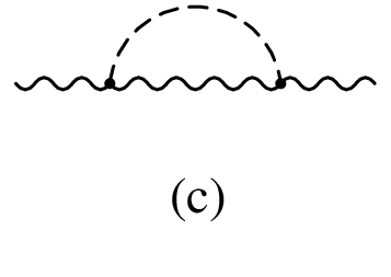
Figure 1: Three types of Feynman diagrams occurring in the calculation of the vacuum polarizations.
Refer to caption
Figure 2: Tadpole diagrams which do not contribute to Δ​ρ\Delta\rho.

In our model, in the computation of the vacuum polarizations of the gauge bosons W±W^{\pm} and Z0Z^{0} there are four types of Feynman diagrams involving scalar fields:

Type (a) diagrams: A scalar branches off from the gauge-boson line and loops back to the same point in that gauge-boson line—see figure 1(a). When the scalar is neutral, the relevant interaction terms in the Lagrangian are the ones in line (29l), for b′=bb^{\prime}=b; but then the contribution to Δ​ρ\Delta\rho vanishes, since one obtains ΠW​Wμ​ν=cW2​ΠZ​Zμ​ν\Pi^{\mu\nu}_{WW}=c_{W}^{2}\Pi^{\mu\nu}_{ZZ}. When the scalar is charged, the relevant terms in the Lagrangian are those in line (29o) for ΠW​Wμ​ν\Pi^{\mu\nu}_{WW} and line (29p) for ΠZ​Zμ​ν\Pi^{\mu\nu}_{ZZ}, in both cases for a′=aa^{\prime}=a.

Type (b) diagrams: The gauge-boson line splits into two scalar lines which later reunite to form a new gauge-boson line—see figure 1(b). The relevant terms in the Lagrangian are those in line (29i) for ΠW​Wμ​ν\Pi^{\mu\nu}_{WW}, and those in lines (29g) and (29h) for ΠZ​Zμ​ν\Pi^{\mu\nu}_{ZZ}.

Type (c) diagrams: A neutral scalar branches off from the gauge-boson line and loops to a later point in that gauge-boson line—see figure 1(c). The interaction terms in the Lagrangian responsible for these Feynman diagrams are those in expression (33).

Type (d) diagrams: A neutral scalar branches off, with zero momentum, from the gauge-boson line, and produces a loop of some stuff—see figure 2. These “tadpole” Feynman diagrams originate from the interaction terms in expression (33). They yield a vanishing contribution to Δ​ρ\Delta\rho since one obtains ΠW​Wμ​ν=cW2​ΠZ​Zμ​ν\Pi^{\mu\nu}_{WW}=c_{W}^{2}\Pi^{\mu\nu}_{ZZ}. Hence we may omit the tadpole diagrams altogether.

3.3 Computation of the loop diagrams

We use dimensional regularization in the computation of the Feynman diagrams. The dimension of space–time is dd. An unphysical mass μ\mu is used to keep the dimension of each integral unchanged when dd varies. We define the divergent quantity

div≡24−d−γ+1+ln⁡(4​π​μ2),\mbox{div}\equiv\frac{2}{4-d}-\gamma+1+\ln{\left(4\pi\mu^{2}\right)},

where γ\gamma is Euler’s constant. In the computation of type (a) Feynman diagrams the relevant momentum integral is

μ4−d​∫dd​k(2​π)d​gμ​νk2−A+i​ε=i​gμ​ν16​π2​A​(div−ln⁡A),\mu^{4-d}\int\frac{\mbox{d}^{d}k}{\left(2\pi\right)^{d}}\,\frac{g^{\mu\nu}}{k^{2}-A+i\varepsilon}=\frac{ig^{\mu\nu}}{16\pi^{2}}\,A\left(\mbox{div}-\ln{A}\right), (36)

where AA is the mass squared of the scalar particle in the loop. In order to compute the type (b) and type (c) Feynman diagrams we need first to introduce a Feynman parameter xx, which is later integrated over from x=0x=0 to x=1x=1. For type (b) diagrams we have

μ4−d​∫dd​k(2​π)d​∫01d​x​4​kμ​kν[k2−A​x−B⁡(1−x)+i​ε]2\displaystyle\mu^{4-d}\int\frac{\mbox{d}^{d}k}{\left(2\pi\right)^{d}}\,\int_{0}^{1}\mbox{d}x\,\frac{4\,k^{\mu}k^{\nu}}{\left[k^{2}-Ax-B\left(1-x\right)+i\varepsilon\right]^{2}} =\displaystyle= i​gμ​ν16​π2[A(div−lnA)\displaystyle\frac{ig^{\mu\nu}}{16\pi^{2}}\left[A\left(\mbox{div}-\ln{A}\right)\right. (37)
+B(div−lnB)+F(A,B)],\displaystyle\left.+B\left(\mbox{div}-\ln{B}\right)+F\left(A,B\right)\right],\hskip 17.07164pt

where AA and BB are the masses squared of the scalars in the loop, and the four-momentum qμq^{\mu} of the external gauge-boson line is taken to obey q2=0q^{2}=0. Notice the presence of terms of the form A⁡(div−ln⁡A)A\left(\mbox{div}-\ln{A}\right) in both diagrams of types (a) and (b); we shall soon see that those terms cancel out in the computation of Δ​ρ\Delta\rho, leaving only the FF functions from the type (b) diagrams. For type (c) diagrams the relevant integral is

μ4−d​∫dd​k(2​π)d​∫01d​x​gμ​ν[k2−A​x−B⁡(1−x)+i​ε]2\displaystyle\mu^{4-d}\int\frac{\mbox{d}^{d}k}{\left(2\pi\right)^{d}}\,\int_{0}^{1}\mbox{d}x\,\frac{g^{\mu\nu}}{\left[k^{2}-Ax-B\left(1-x\right)+i\varepsilon\right]^{2}} =\displaystyle= i​gμ​ν16​π21A[A(div−lnA)−A+B2\displaystyle\frac{ig^{\mu\nu}}{16\pi^{2}}\,\frac{1}{A}\left[A\left(\mbox{div}-\ln{A}\right)-\frac{A+B}{2}\right. (38)
+F(A,B)].\displaystyle\left.+F\left(A,B\right)\right].

This integral is symmetric under the interchange of AA and BB; equation (38) presents a seemingly asymmetric form, but it is in fact symmetric. The reason for expressing the integral in this way is that, due to cancellations, only the terms F⁡(A,B)F\left(A,B\right) survive in the end.

3.4 The contributions to Δ​ρ\Delta\rho from diagrams of types (a) and (b)

Using (29o) and (36), we see that the contribution to AW​W​(q2)A_{WW}\left(q^{2}\right) of type (a) Feynman diagrams with charged scalars in the loop is

AW​W(a)(q2)=−g232​π2∑a=1n(U†U)a​ama2(div−lnma2).A^{(a)}_{WW}\left(q^{2}\right)=-\frac{g^{2}}{32\pi^{2}}\,\sum_{a=1}^{n}\left(U^{\dagger}U\right)_{aa}m_{a}^{2}\left(\mbox{div}-\ln{m_{a}^{2}}\right). (39)

In the same way, using (29p),

AZ​Z(a)(q2)=−g232​π2​cW2∑a=1n[4sW4+(1−4sW2)(U†U)a​a]ma2(div−lnma2).A^{(a)}_{ZZ}\left(q^{2}\right)=-\frac{g^{2}}{32\pi^{2}c_{W}^{2}}\,\sum_{a=1}^{n}\left[4s_{W}^{4}+\left(1-4s_{W}^{2}\right)\left(U^{\dagger}U\right)_{aa}\right]m_{a}^{2}\left(\mbox{div}-\ln{m_{a}^{2}}\right). (40)

Proceeding to the type (b) Feynman diagrams, from (29i) and (37) we find that

AW​W(b)​(0)\displaystyle A^{(b)}_{WW}\left(0\right) =\displaystyle= g264​π2∑a=1n∑b=1m(U†V)a​b(V†U)b​a[ma2(div−lnma2)\displaystyle\frac{g^{2}}{64\pi^{2}}\,\sum_{a=1}^{n}\sum_{b=1}^{m}\left(U^{\dagger}V\right)_{ab}\left(V^{\dagger}U\right)_{ba}\left[m_{a}^{2}\left(\mbox{div}-\ln{m_{a}^{2}}\right)\right. (41a)
+μb2(div−lnμb2)+F(ma2,μb2)]\displaystyle\left.+\mu_{b}^{2}\left(\mbox{div}-\ln{\mu_{b}^{2}}\right)+F\left(m_{a}^{2},\mu_{b}^{2}\right)\right]
=\displaystyle= g264​π2[2∑a=1n(U†U)a​ama2(div−lnma2)\displaystyle\frac{g^{2}}{64\pi^{2}}\left[2\sum_{a=1}^{n}\left(U^{\dagger}U\right)_{aa}m_{a}^{2}\left(\mbox{div}-\ln{m_{a}^{2}}\right)\right.
+∑b=1m(V†V)b​bμb2(div−lnμb2)\displaystyle+\sum_{b=1}^{m}\left(V^{\dagger}V\right)_{bb}\mu_{b}^{2}\left(\mbox{div}-\ln{\mu_{b}^{2}}\right) (41b)
+∑a=1n∑b=1m|(U†V)a​b|2F(ma2,μb2)].\displaystyle\left.+\sum_{a=1}^{n}\sum_{b=1}^{m}\left|\left(U^{\dagger}V\right)_{ab}\right|^{2}F\left(m_{a}^{2},\mu_{b}^{2}\right)\right]. (41c)

We have used

∑a=1n(U†​V)a​b​(V†​U)b​a=(V†​V)b​b,\sum_{a=1}^{n}\left(U^{\dagger}V\right)_{ab}\left(V^{\dagger}U\right)_{ba}=\left(V^{\dagger}V\right)_{bb}, (42)

which follows from the unitarity of U~\tilde{U}, i.e. from [21]

U​U†=1nd×nd.UU^{\dagger}=1_{n_{d}\times n_{d}}. (43)

We have also used

∑b=1m(U†​V)a​b​(V†​U)b​a=2​(U†​U)a​a,\sum_{b=1}^{m}\left(U^{\dagger}V\right)_{ab}\left(V^{\dagger}U\right)_{ba}=2\left(U^{\dagger}U\right)_{aa}, (44)

which follows from the orthogonality of V~\tilde{V}, i.e. from [21]

Re​V​Re​VT=Im​V​Im​VT=1nd×nd,Re​V​Im​VT=Im​V​Re​VT=0nd×nd.\begin{array}[]{rcccl}\mbox{Re}\,V\ \mbox{Re}V^{T}&=&\mbox{Im}\,V\ \mbox{Im}V^{T}&=&1_{n_{d}\times n_{d}},\\[2.84526pt] \mbox{Re}\,V\ \mbox{Im}V^{T}&=&\mbox{Im}\,V\ \mbox{Re}V^{T}&=&0_{n_{d}\times n_{d}}.\end{array} (45)

Considering now the self-energy of the Z0Z^{0} boson, we find

AZ​Z(b)​(0)\displaystyle A_{ZZ}^{(b)}\left(0\right) =\displaystyle= g264​π2​cW2{∑a,a′=1n[2sW2δa​a′−(U†U)a′​a][2sW2δa​a′−(U†U)a​a′]\displaystyle\frac{g^{2}}{64\pi^{2}c_{W}^{2}}\left\{\sum_{a,a^{\prime}=1}^{n}\left[2s_{W}^{2}\delta_{aa^{\prime}}-\left(U^{\dagger}U\right)_{a^{\prime}a}\right]\left[2s_{W}^{2}\delta_{aa^{\prime}}-\left(U^{\dagger}U\right)_{aa^{\prime}}\right]\right. (46a)
×[ma2​(div−ln⁡ma2)+ma′2​(div−ln⁡ma′2)+F⁡(ma2,ma′2)]\displaystyle\times\left[m_{a}^{2}\left(\mbox{div}-\ln{m_{a}^{2}}\right)+m_{a^{\prime}}^{2}\left(\mbox{div}-\ln{m_{a^{\prime}}^{2}}\right)+F\left(m_{a}^{2},m_{a^{\prime}}^{2}\right)\right]
+∑b=1m−1∑b′=b+1m[Im(V†V)b​b′]2\displaystyle+\sum_{b=1}^{m-1}\sum_{b^{\prime}=b+1}^{m}\left[\mbox{Im}\left(V^{\dagger}V\right)_{bb^{\prime}}\right]^{2}
×[μb2(div−lnμb2)+μb′2(div−lnμb′2)+F(μb2,μb′2)]}\displaystyle\left.\times\left[\mu_{b}^{2}\left(\mbox{div}-\ln{\mu_{b}^{2}}\right)+\mu_{b^{\prime}}^{2}\left(\mbox{div}-\ln{\mu_{b^{\prime}}^{2}}\right)+F\left(\mu_{b}^{2},\mu_{b^{\prime}}^{2}\right)\right]\right\}
=\displaystyle= g264​π2​cW2{2∑a=1n−1∑a′=a+1n|(U†U)a​a′|2F(ma2,ma′2)\displaystyle\frac{g^{2}}{64\pi^{2}c_{W}^{2}}\left\{2\,\sum_{a=1}^{n-1}\sum_{a^{\prime}=a+1}^{n}\left|\left(U^{\dagger}U\right)_{aa^{\prime}}\right|^{2}F\left(m_{a}^{2},m_{a^{\prime}}^{2}\right)\right.
+2∑a=1n[4sW4+(1−4sW2)(U†U)a​a]ma2(div−lnma2)\displaystyle+2\,\sum_{a=1}^{n}\left[4s_{W}^{4}+\left(1-4s_{W}^{2}\right)\left(U^{\dagger}U\right)_{aa}\right]m_{a}^{2}\left(\mbox{div}-\ln{m_{a}^{2}}\right) (46b)
+∑b=1m−1∑b′=b+1m[Im(V†V)b​b′]2F(μb2,μb′2)\displaystyle+\sum_{b=1}^{m-1}\sum_{b^{\prime}=b+1}^{m}\left[\mbox{Im}\left(V^{\dagger}V\right)_{bb^{\prime}}\right]^{2}F\left(\mu_{b}^{2},\mu_{b^{\prime}}^{2}\right) (46c)
+∑b=1m(V†V)b​bμb2(div−lnμb2)}.\displaystyle\left.+\sum_{b=1}^{m}\left(V^{\dagger}V\right)_{bb}\mu_{b}^{2}\left(\mbox{div}-\ln{\mu_{b}^{2}}\right)\right\}. (46d)

We have used

∑b′=1m[Im​(V†​V)b​b′]2=(V†​V)b​b,\sum_{b^{\prime}=1}^{m}\left[\mbox{Im}\left(V^{\dagger}V\right)_{bb^{\prime}}\right]^{2}=\left(V^{\dagger}V\right)_{bb}, (47)

which follows from equations (45).

Putting everything together, we see that

the AW​W(a)​(q2)A^{(a)}_{WW}\left(q^{2}\right) of equation (39) cancels out the line (41a) of AW​W(b)​(0)A^{(b)}_{WW}\left(0\right);

the AZ​Z(a)​(q2)A^{(a)}_{ZZ}\left(q^{2}\right) of equation (40) cancels out the line (46b) of AZ​Z(b)​(0)A^{(b)}_{ZZ}\left(0\right);

the line (41b) of AW​W(b)​(0)A^{(b)}_{WW}\left(0\right) cancels out the line (46d) of AZ​Z(b)​(0)A^{(b)}_{ZZ}\left(0\right) in the subtraction AW​W−cW2​AZ​ZA_{WW}-c_{W}^{2}A_{ZZ}.

In this way we finally obtain

AW​W(a+b)​(0)−cW2​AZ​Z(a+b)​(0)\displaystyle A^{(a+b)}_{WW}\left(0\right)-c_{W}^{2}A^{(a+b)}_{ZZ}\left(0\right) =\displaystyle= g264​π2{∑a=1n∑b=1m|(U†V)a​b|2F(ma2,μb2)\displaystyle\frac{g^{2}}{64\pi^{2}}\left\{\sum_{a=1}^{n}\sum_{b=1}^{m}\left|\left(U^{\dagger}V\right)_{ab}\right|^{2}F\left(m_{a}^{2},\mu_{b}^{2}\right)\right. (48a)
−2∑a=1n−1∑a′=a+1n|(U†U)a​a′|2F(ma2,ma′2)\displaystyle-2\,\sum_{a=1}^{n-1}\sum_{a^{\prime}=a+1}^{n}\left|\left(U^{\dagger}U\right)_{aa^{\prime}}\right|^{2}F\left(m_{a}^{2},m_{a^{\prime}}^{2}\right) (48b)
−∑b=1m−1∑b′=b+1m[Im(V†V)b​b′]2F(μb2,μb′2)}.\displaystyle\left.-\sum_{b=1}^{m-1}\sum_{b^{\prime}=b+1}^{m}\left[\mbox{Im}\left(V^{\dagger}V\right)_{bb^{\prime}}\right]^{2}F\left(\mu_{b}^{2},\mu_{b^{\prime}}^{2}\right)\right\}.\hskip 8.53581pt (48c)

The positive term (48a) originates from AW​W(b)A^{(b)}_{WW} while the negative terms (48b) and (48c) come from AZ​Z(b)A^{(b)}_{ZZ}.

If there are in the electroweak theory any scalar S​U​(2)SU(2) singlets with electric charges other than 00 or ±1\pm 1, then the relevant terms in the Lagrangian are those in equation (35). The term (35b) generates a type (a) Feynman diagram which exactly cancels the type (b) Feynman diagram generated by the term (35a).77 7 This cancellation is analogous to the one between equation (40) and line (46b). Thus, scalar S​U​(2)SU(2) singlets with electric charge different from 00 and ±1\pm 1 do not affect Δ​ρ\Delta\rho at all.

The sums in equation (48) include contributions from the Goldstone bosons G±=S1±G^{\pm}=S_{1}^{\pm} and G0=S10G^{0}=S^{0}_{1}. These Goldstone bosons have unphysical masses m1m_{1} and μ1\mu_{1}, respectively, which are arbitrary in a ’t Hooft gauge. The terms which depend on those masses are, explicitly,

|(U†​V)11|2​F​(m12,μ12)\displaystyle\left|\left(U^{\dagger}V\right)_{11}\right|^{2}F\left(m_{1}^{2},\mu_{1}^{2}\right) (49a)
+∑b=2m|(U†V)1​b|2F(m12,μb2)\displaystyle+\sum_{b=2}^{m}\left|\left(U^{\dagger}V\right)_{1b}\right|^{2}F\left(m_{1}^{2},\mu_{b}^{2}\right) (49b)
+∑a=2n|(U†V)a​1|2F(ma2,μ12)\displaystyle+\sum_{a=2}^{n}\left|\left(U^{\dagger}V\right)_{a1}\right|^{2}F\left(m_{a}^{2},\mu_{1}^{2}\right) (49c)
−2∑a=2n|(U†U)1​a|2F(m12,ma2)\displaystyle-2\,\sum_{a=2}^{n}\left|\left(U^{\dagger}U\right)_{1a}\right|^{2}F\left(m_{1}^{2},m_{a}^{2}\right) (49d)
−∑b=2m[Im(V†V)1​b]2F(μ12,μb2).\displaystyle-\sum_{b=2}^{m}\left[\mbox{Im}\left(V^{\dagger}V\right)_{1b}\right]^{2}F\left(\mu_{1}^{2},\mu_{b}^{2}\right). (49e)

One may eliminate some of these terms by using equations (30) and (31). Indeed, (U†​U)1​a=−(T†​T)1​a=0\left(U^{\dagger}U\right)_{1a}=-\left(T^{\dagger}T\right)_{1a}=0 when a≠1a\neq 1, because Tj​1=0T_{j1}=0 for any jj; also, (U†​V)a​1=i​(U†​U)a​1=0\left(U^{\dagger}V\right)_{a1}=i\left(U^{\dagger}U\right)_{a1}=0 for a≠1a\neq 1. Therefore, the terms (49c) and (49d) vanish. In the term (49a), (U†​V)11=i\left(U^{\dagger}V\right)_{11}=i. In the term (49b) one may write

(U†​V)1​b=i​(V†​V)1​b=−Im​(V†​V)1​b⇐b≠1,\left(U^{\dagger}V\right)_{1b}=i\left(V^{\dagger}V\right)_{1b}=-\mbox{Im}\left(V^{\dagger}V\right)_{1b}\ \Leftarrow b\neq 1, (50)

since Re​(V†​V)1​b=(Re​VT​Re​V+Im​VT​Im​V)1​b=−(RT​R)1​b=0\mbox{Re}\left(V^{\dagger}V\right)_{1b}=\left(\mbox{Re}\,V^{T}\ \mbox{Re}\,V+\mbox{Im}\,V^{T}\ \mbox{Im}\,V\right)_{1b}=-\left(R^{T}R\right)_{1b}=0. In this way, the terms (49) are reduced to

F⁡(m12,μ12)+∑b=2m[Im​(V†​V)1​b]2​[F⁡(m12,μb2)−F⁡(μ12,μb2)].F\left(m_{1}^{2},\mu_{1}^{2}\right)+\sum_{b=2}^{m}\left[\mbox{Im}\left(V^{\dagger}V\right)_{1b}\right]^{2}\left[F\left(m_{1}^{2},\mu_{b}^{2}\right)-F\left(\mu_{1}^{2},\mu_{b}^{2}\right)\right]. (51)

The term F⁡(m12,μ12)F\left(m_{1}^{2},\mu_{1}^{2}\right) is independent of the number of scalar doublets and singlets, hence it is eliminated when one subtracts the SM result from the Multi-Higgs-doublet-model one. The other terms in the expression (51) are cancelled out by the diagrams of type (c), as we shall see next.

3.5 The contributions to Δ​ρ\Delta\rho from diagrams of type (c)

To compensate for the unphysical masses of the Goldstone bosons, the propagators of gauge bosons W±W^{\pm} and Z0Z^{0} with four-momentum kμk^{\mu} are, in a ’t Hooft gauge,

−kμ​kνmW2​ik2−m12+(−gμ​ν+kμ​kνmW2)​ik2−mW2,\displaystyle-\frac{k_{\mu}k_{\nu}}{m_{W}^{2}}\,\frac{i}{k^{2}-m_{1}^{2}}+\left(-g_{\mu\nu}+\frac{k_{\mu}k_{\nu}}{m_{W}^{2}}\right)\frac{i}{k^{2}-m_{W}^{2}}, (52)
−kμ​kνmZ2​ik2−μ12+(−gμ​ν+kμ​kνmZ2)​ik2−mZ2,\displaystyle-\frac{k_{\mu}k_{\nu}}{m_{Z}^{2}}\,\frac{i}{k^{2}-\mu_{1}^{2}}+\left(-g_{\mu\nu}+\frac{k_{\mu}k_{\nu}}{m_{Z}^{2}}\right)\frac{i}{k^{2}-m_{Z}^{2}}, (53)

respectively, i.e. they contain a piece with a pole on the unphysical masses squared m12m_{1}^{2} and μ12\mu_{1}^{2}, respectively.

Using these propagators to compute the type (c) Feynman diagrams, one obtains

AW​W(c)​(0)\displaystyle A^{(c)}_{WW}\left(0\right) =\displaystyle= g264​π2∑b=2m[Im(V†V)1​b]2[−m12(div−lnm12)−3mW2(div−lnmW2)\displaystyle\frac{g^{2}}{64\pi^{2}}\,\sum_{b=2}^{m}\left[\mbox{Im}\left(V^{\dagger}V\right)_{1b}\right]^{2}\left[-m_{1}^{2}\left(\mbox{div}-\ln{m_{1}^{2}}\right)-3m_{W}^{2}\left(\mbox{div}-\ln{m_{W}^{2}}\right)\right. (54)
+2(mW2+μb2)−F(m12,μb2)−3F(mW2,μb2)],\displaystyle\left.+2\left(m_{W}^{2}+\mu_{b}^{2}\right)-F\left(m_{1}^{2},\mu_{b}^{2}\right)-3F\left(m_{W}^{2},\mu_{b}^{2}\right)\right],
AZ​Z(c)​(0)\displaystyle A^{(c)}_{ZZ}\left(0\right) =\displaystyle= g264​π2​cW2∑b=2m[Im(V†V)1​b]2[−μ12(div−lnμ12)−3mZ2(div−lnmZ2)\displaystyle\frac{g^{2}}{64\pi^{2}c_{W}^{2}}\,\sum_{b=2}^{m}\left[\mbox{Im}\left(V^{\dagger}V\right)_{1b}\right]^{2}\left[-\mu_{1}^{2}\left(\mbox{div}-\ln{\mu_{1}^{2}}\right)-3m_{Z}^{2}\left(\mbox{div}-\ln{m_{Z}^{2}}\right)\right. (55)
+2(mZ2+μb2)−F(μ12,μb2)−3F(mZ2,μb2)].\displaystyle\left.+2\left(m_{Z}^{2}+\mu_{b}^{2}\right)-F\left(\mu_{1}^{2},\mu_{b}^{2}\right)-3F\left(m_{Z}^{2},\mu_{b}^{2}\right)\right].

The factors 33 originate in a partial cancellation between the contributions from the pieces −gμ​ν-g_{\mu\nu} and kμ​kν/mV2k_{\mu}k_{\nu}/m_{V}^{2} in the propagator of the gauge boson VV, the former contribution being four times larger than, and with opposite sign relative to, the latter one, cf. equations (37) and (38). Performing the subtraction relevant for Δ​ρ\Delta\rho, one obtains

AW​W(c)​(0)−cW2​AZ​Z(c)​(0)\displaystyle A^{(c)}_{WW}\left(0\right)-c_{W}^{2}A^{(c)}_{ZZ}\left(0\right) =\displaystyle= g264​π2​∑b=2m[Im​(V†​V)1​b]2\displaystyle\frac{g^{2}}{64\pi^{2}}\,\sum_{b=2}^{m}\left[\mbox{Im}\left(V^{\dagger}V\right)_{1b}\right]^{2} (56a)
×[−m12(div−lnm12)+μ12(div−lnμ12)\displaystyle\times\left[-m_{1}^{2}\left(\mbox{div}-\ln{m_{1}^{2}}\right)+\mu_{1}^{2}\left(\mbox{div}-\ln{\mu_{1}^{2}}\right)\right.
−3​mW2​(div−ln⁡mW2)+3​mZ2​(div−ln⁡mZ2)\displaystyle-3m_{W}^{2}\left(\mbox{div}-\ln{m_{W}^{2}}\right)+3m_{Z}^{2}\left(\mbox{div}-\ln{m_{Z}^{2}}\right)\hskip 11.38109pt (56b)
+2​(mW2−mZ2)\displaystyle+2\left(m_{W}^{2}-m_{Z}^{2}\right) (56c)
−F⁡(m12,μb2)+F⁡(μ12,μb2)\displaystyle-F\left(m_{1}^{2},\mu_{b}^{2}\right)+F\left(\mu_{1}^{2},\mu_{b}^{2}\right) (56d)
−3F(mW2,μb2)+3F(mZ2,μb2)].\displaystyle\left.-3F\left(m_{W}^{2},\mu_{b}^{2}\right)+3F\left(m_{Z}^{2},\mu_{b}^{2}\right)\right]. (56e)

The terms (56a)–(56c) are independent of the number of scalar doublets. They disappear when one subtracts the Standard-Model result from the multi-Higgs-doublet-model one, since

∑b=2m[Im​(V†​V)1​b]2=(V†​V)11=1.\sum_{b=2}^{m}\left[\mbox{Im}\left(V^{\dagger}V\right)_{1b}\right]^{2}=\left(V^{\dagger}V\right)_{11}=1. (57)

The terms (56d), which involve the masses of the Goldstone bosons, cancel out the terms in (51), except the first one, which is cancelled by the subtraction of the SM result.

We have thus finished the derivation of equation (23) for Δ​ρ\Delta\rho.

4 The 2HDM and the Zee model

In this section we give, as examples of the application of our general formulae, the expressions for Δ​ρ\Delta\rho in the 2HDM and also in the model of Zee [24] for the radiative generation of neutrino masses, which has one singly charged S​U​(2)SU(2) singlet together with the two doublets.

In the study of the 2HDM it is convenient to use the so-called “Higgs basis,” in which only the first Higgs doublet has a vacuum expectation value. In that basis,

ϕ1=(G+(v+H+i​G0)/2),ϕ2=(S2+(R+i​I)/2).\phi_{1}=\left(\begin{array}[]{c}G^{+}\\ \left(v+H+iG^{0}\right)\left/\sqrt{2}\right.\end{array}\right),\quad\phi_{2}=\left(\begin{array}[]{c}S_{2}^{+}\\ \left(R+iI\right)\left/\sqrt{2}\right.\end{array}\right). (58)

Here, G+≡S1+G^{+}\equiv S_{1}^{+} and G0≡S10G^{0}\equiv S_{1}^{0} are the Goldstone bosons, while S2+S_{2}^{+} is the physical charged scalar, which has mass m2m_{2}. Thus, the matrix UU, which connects the charged components of ϕ1\phi_{1} and ϕ2\phi_{2} to the eigenstates of mass, is in the Higgs basis of the 2HDM equal to the unit matrix. On the other hand, HH, RR and II, which are real fields, must be rotated through a 3×33\times 3 orthogonal matrix OO to obtain the three physical neutral fields S2,3,40S^{0}_{2,3,4}:

(HRI)=O​(S20S30S40).\left(\begin{array}[]{c}H\\ R\\ I\end{array}\right)=O\left(\begin{array}[]{c}S_{2}^{0}\\ S_{3}^{0}\\ S_{4}^{0}\end{array}\right). (59)

Without lack of generality we choose detO=+1\det{O}=+1. Thus, the 2×42\times 4 matrix VV, defined through

(H+i​G0R+i​I)=V​(G0S20S30S40),\left(\begin{array}[]{c}H+iG^{0}\\ R+iI\end{array}\right)=V\left(\begin{array}[]{c}G^{0}\\ S_{2}^{0}\\ S_{3}^{0}\\ S_{4}^{0}\end{array}\right), (60)

is

V=(iO11O12O130O21+i​O31O22+i​O32O23+i​O33).V=\left(\begin{array}[]{cccc}i&O_{11}&O_{12}&O_{13}\\ 0&O_{21}+iO_{31}&O_{22}+iO_{32}&O_{23}+iO_{33}\end{array}\right). (61)

Therefore,

V†​V=(1−i​O11−i​O12−i​O13i​O111i​O13−i​O12i​O12−i​O131i​O11i​O13i​O12−i​O111).V^{\dagger}V=\left(\begin{array}[]{cccc}1&-iO_{11}&-iO_{12}&-iO_{13}\\ iO_{11}&1&iO_{13}&-iO_{12}\\ iO_{12}&-iO_{13}&1&iO_{11}\\ iO_{13}&iO_{12}&-iO_{11}&1\end{array}\right). (62)

The value of Δ​ρ\Delta\rho in the 2HDM is therefore, using our formula in equation (25),

Δ​ρ\displaystyle\Delta\rho =\displaystyle= g264​π2​mW2{∑b=24(1−O1​b−12)F(m22,μb2)\displaystyle\frac{g^{2}}{64\pi^{2}m_{W}^{2}}\left\{\sum_{b=2}^{4}\left(1-O_{1\,b-1}^{2}\right)F\left(m_{2}^{2},\mu_{b}^{2}\right)\right. (63)
−O132​F​(μ22,μ32)−O122​F​(μ22,μ42)−O112​F​(μ32,μ42)\displaystyle-O_{13}^{2}F\left(\mu_{2}^{2},\mu_{3}^{2}\right)-O_{12}^{2}F\left(\mu_{2}^{2},\mu_{4}^{2}\right)-O_{11}^{2}F\left(\mu_{3}^{2},\mu_{4}^{2}\right)
+3∑b=24O1​b−12[F(mZ2,μb2)−F(mW2,μb2)−F(mZ2,mh2)+F(mW2,mh2)]},\displaystyle\left.+3\sum_{b=2}^{4}O_{1\,b-1}^{2}\left[F\left(m_{Z}^{2},\mu_{b}^{2}\right)-F\left(m_{W}^{2},\mu_{b}^{2}\right)-F\left(m_{Z}^{2},m_{h}^{2}\right)+F\left(m_{W}^{2},m_{h}^{2}\right)\right]\right\},\hskip 19.91692pt

where μ2,3,4\mu_{2,3,4} denote the the masses of S2,3,40S^{0}_{2,3,4}, respectively, while mhm_{h} is the mass of the Higgs boson of the SM. Equation (63) reproduces, in a somewhat simplified form, the result for Δ​ρ\Delta\rho in the 2HDM previously given in [16].

A special case of the 2HDM is the model with one “dark” scalar doublet. This means that a second doublet is added to the SM, but that doublet has no VEV and it does not mix with the standard Higgs doublet [19]. We should then identify HH with the usual Higgs particle. Thus, O11=1O_{11}=1 and μ2=mh\mu_{2}=m_{h}. Equation (63) then simplifies to [25, 20]

Δ​ρ=g264​π2​mW2​[∑b=34F⁡(m22,μb2)−F⁡(μ32,μ42)].\Delta\rho=\frac{g^{2}}{64\pi^{2}m_{W}^{2}}\left[\sum_{b=3}^{4}F\left(m_{2}^{2},\mu_{b}^{2}\right)-F\left(\mu_{3}^{2},\mu_{4}^{2}\right)\right]. (64)

This quantity is small if the three masses m2m_{2}, μ3\mu_{3} and μ4\mu_{4} are close together. Notice that in this case of a “dark” scalar doublet there are no vector–vector–scalar couplings involving the additional doublet, hence Δ​ρ\Delta\rho stems exclusively from type (a) and type (b) Feynman diagrams.

In the model of Zee there is, besides the two scalar S​U​(2)SU(2) doublets

ϕ1=(G+(v+H+i​G0)/2),ϕ2=(H+(R+i​I)/2),\phi_{1}=\left(\begin{array}[]{c}G^{+}\\ \left(v+H+iG^{0}\right)\left/\sqrt{2}\right.\end{array}\right),\quad\phi_{2}=\left(\begin{array}[]{c}H^{+}\\ \left(R+iI\right)\left/\sqrt{2}\right.\end{array}\right), (65)

also one scalar S​U​(2)SU(2) singlet χ+\chi^{+} with unit electric charge. Therefore there is a 2×22\times 2 unitary matrix KK such that

(H+χ+)=K​(S2+S3+),\left(\begin{array}[]{c}H^{+}\\ \chi^{+}\end{array}\right)=K\left(\begin{array}[]{c}S_{2}^{+}\\ S_{3}^{+}\end{array}\right), (66)

where S2+S_{2}^{+} and S3+S_{3}^{+} are the physical charged scalars, which have masses m2m_{2} and m3m_{3}, respectively. So, now the matrix UU of equation (15) is

U=(1000K11K12),U=\left(\begin{array}[]{ccc}1&0&0\\ 0&K_{11}&K_{12}\end{array}\right), (67)

so that

U†​U=(1000|K11|2K11∗​K120K11​K12∗|K12|2).U^{\dagger}U=\left(\begin{array}[]{ccc}1&0&0\\ 0&\left|K_{11}\right|^{2}&K_{11}^{\ast}K_{12}\\ 0&K_{11}K_{12}^{\ast}&\left|K_{12}\right|^{2}\end{array}\right). (68)

Equations (61) and (62) retain their validity, and

U†​V=(iO11O12O130K11∗​(O21+i​O31)K11∗​(O22+i​O32)K11∗​(O23+i​O33)0K12∗​(O21+i​O31)K12∗​(O22+i​O32)K12∗​(O23+i​O33)).U^{\dagger}V=\left(\begin{array}[]{cccc}i&O_{11}&O_{12}&O_{13}\\ 0&K_{11}^{*}\left(O_{21}+iO_{31}\right)&K_{11}^{*}\left(O_{22}+iO_{32}\right)&K_{11}^{*}\left(O_{23}+iO_{33}\right)\\ 0&K_{12}^{*}\left(O_{21}+iO_{31}\right)&K_{12}^{*}\left(O_{22}+iO_{32}\right)&K_{12}^{*}\left(O_{23}+iO_{33}\right)\end{array}\right). (69)

Therefore, using our general formula (23) for Δ​ρ\Delta\rho, we see that, in the model of Zee,

Δ​ρ\displaystyle\Delta\rho =\displaystyle= g264​π2​mW2{∑b=24(1−O1​b−12)∑a=23|K1​a−1|2F(ma2,μb2)\displaystyle\frac{g^{2}}{64\pi^{2}m_{W}^{2}}\left\{\sum_{b=2}^{4}\left(1-O_{1\,b-1}^{2}\right)\sum_{a=2}^{3}\left|K_{1\,a-1}\right|^{2}F\left(m_{a}^{2},\mu_{b}^{2}\right)\right. (70)
−2​|K11​K12|2​F​(m22,m32)\displaystyle-2\left|K_{11}K_{12}\right|^{2}F\left(m_{2}^{2},m_{3}^{2}\right)
−O132​F​(μ22,μ32)−O122​F​(μ22,μ42)−O112​F​(μ32,μ42)\displaystyle-O_{13}^{2}F\left(\mu_{2}^{2},\mu_{3}^{2}\right)-O_{12}^{2}F\left(\mu_{2}^{2},\mu_{4}^{2}\right)-O_{11}^{2}F\left(\mu_{3}^{2},\mu_{4}^{2}\right)
+3∑b=24O1​b−12[F(mZ2,μb2)−F(mW2,μb2)−F(mZ2,mh2)+F(mW2,mh2)]}.\displaystyle\left.+3\sum_{b=2}^{4}O_{1\,b-1}^{2}\left[F\left(m_{Z}^{2},\mu_{b}^{2}\right)-F\left(m_{W}^{2},\mu_{b}^{2}\right)-F\left(m_{Z}^{2},m_{h}^{2}\right)+F\left(m_{W}^{2},m_{h}^{2}\right)\right]\right\}.\hskip 19.91692pt

5 Summary

In this paper we have derived the formula for the parameter Δ​ρ\Delta\rho, as defined in equation (4), in an extension of the Standard Model characterized by an arbitrary number of scalar S​U​(2)SU(2) doublets (with hypercharge ±1/2\pm 1/2) and singlets (with arbitrary hypercharges). Our formalism is completely general, using only the masses of the scalars and their mixing matrices, which ensures that our formulae are always applicable. The computation has been carried out in a general RξR_{\xi} gauge, thereby demonstrating that the final result is independent of the masses of the unphysical scalars. We have also explicitly demonstrated that all infinities cancel out in the final result for Δ​ρ\Delta\rho. In order to ease the consultation of this paper, the formulae for Δ​ρ\Delta\rho given in Section 2 have been completely separated from their derivation presented in Section 3. Our results can be applied either to check the viability of a model or to constrain its parameter space, by comparing the Δ​ρ\Delta\rho, calculated in that model, with numerical bounds on Δ​ρ\Delta\rho obtained from a fit to precision data—for instance, the bound (7) found in [4]. As an illustration of our general formulae, in Section 4 we have worked out the specific cases of the two-Higgs-doublet model, with and without one extra charged scalar singlet.

Acknowledgements:

W.G. thanks S. Dittmaier, W. Hollik, M. Krawczyk and H. Neufeld for helpful discussions. The work of L.L. was supported by the Portuguese Fundação para a Ciência e a Tecnologia through the project U777–Plurianual. W.G. and L.L. acknowledge support from EU under the MRTN-CT-2006-035505 network programme.

References

  • [1] D.A. Ross and M.J.G. Veltman, Neutral currents in neutrino experiments, Nucl. Phys. B 95 (1975) 135;
    M.J.G. Veltman, Second threshold in weak interactions, Acta Phys. Polon. B 8 (1977) 475;
    M.J.G. Veltman, Limit on mass differences in the Weinberg model, Nucl. Phys. B 123 (1977) 89.
  • [2] M.B. Einhorn, D.R.T. Jones and M.J.G. Veltman, Heavy particles and the rho parameter in the Standard Model, Nucl. Phys. B 191 (1981) 146.
  • [3] W.M. Yao et al. (Particle Data Group), Review of particle physics, J. Phys. G (Particles and Fields) 33 (2006) 1.
  • [4] J. Erler and P. Langacker in [3], p. 119.
  • [5] S. Bertolini, Quantum effects in a two-Higgs-doublet model of the electroweak interactions, Nucl. Phys. B 272 (1986) 77.
  • [6] A. Denner, R.J. Guth and J.H. Kühn, Relaxation of top-mass limits in the two-Higgs-doublet model, Phys. Lett. B 240 (1990) 438;
    C.D. Froggatt, R.G. Moorhouse and I.G. Knowles, Leading radiative corrections in two-scalar-doublet models, Phys. Rev. D 45 (1992) 2471.
  • [7] R. Boughezal, J.B. Tausk and J.J. van der Bij, Three-loop electroweak correction to the rho parameter in the large Higgs mass limit, Nucl. Phys. B 713 (2005) 278 [hep-ph/0410216], and references therein.
  • [8] M.E. Peskin and T. Takeuchi, A new constraint on a strongly interacting Higgs sector, Phys. Rev. Lett. 65 (1990) 964;
    M.E. Peskin and T. Takeuchi, Estimation of oblique electroweak corrections, Phys. Rev. D 46 (1992) 381.
  • [9] G. Altarelli and R. Barbieri, Vacuum-polarization effects of new physics on electroweak processes, Phys. Lett. B 253 (1991) 161;
    G. Altarelli, R. Barbieri and S. Jadach, Toward a model-independent analysis of electroweak data, Nucl. Phys. B 369 (1992) 3 [erratum ibid. B 376 (1992) 444].
  • [10] I. Maksymyk, C.P. Burgess and D. London, Beyond S, T, and U, Phys. Rev. D 50 (1994) 529 [hep-ph/9306267].
  • [11] J.F. Gunion, H.E. Haber, G.L. Kane and S. Dawson, The Higgs hunter’s guide, Addision–Wesley Publishing Company, Reading (Massachusetts) 1989.
  • [12] W. Hollik, Nonstandard Higgs bosons in S​U​(2)×U⁡(1)SU(2)\times U(1) radiative corrections, Z. Phys. C 32 (1986) 291;
    W. Hollik, Radiative corrections with two Higgs doublets at LEP/SLC and HERA, Z. Phys. C 37 (1988) 569;
    A. Denner, R.J. Guth, W. Hollik and J.H. Kühn, The ZZ width in the two-Higgs-doublet model, Z. Phys. C 51 (1991) 695.
  • [13] P.H. Chankowski, M. Krawczyk and J. Żochowski, Implications of the precision data for very light Higgs boson scenarios in 2HDM(II), Eur. Phys. J. C 11 (1999) 661 [hep-ph/9905436].
  • [14] P.H. Chankowski, T. Farris, B. Grzadkowski, J.F. Gunion, J. Kalinowski and M. Krawczyk, Do precision electroweak constraints guarantee e+​e−e^{+}e^{-} collider discovery of at least one Higgs boson of a two-Higgs-doublet model?, Phys. Lett. B 496 (2000) 195 [hep-ph/0009271];
    M. Krawczyk and D. Temes, Large 2HDM(II) one-loop corrections in leptonic tau decays, Eur. Phys. J. C 44 (2005) 435 [hep-ph/0410248].
  • [15] J.F. Gunion and H.E. Haber, The CP-conserving two-Higgs-doublet model: the approach to the decoupling limit, Phys. Rev. D 67 (2003) 075019 [hep-ph/0207010];
    K. Cheung and O.C.W. Kong, Can the two-Higgs-doublet model survive the constraints from the muon anomalous magnetic moment as suggested?, Phys. Rev. D 68 (2003) 053003 [hep-ph/0302111].
  • [16] A.W. El Kaffas, W. Khater, O.M. Ogreid and P. Osland, Consistency of the two-Higgs-doublet model and CP violation in top production at the LHC, Nucl. Phys. B 775 (2007) 45 [hep-ph/0605142].
  • [17] Y. Grossman, Phenomenology of models with more than two Higgs doublets, Nucl. Phys. B 426 (1994) 355 [hep-ph/9401311].
  • [18] W. Grimus, Neutrino physics—Theory, in Lectures on flavor physics, U.-G. Meißner and W. Plessas eds., Springer Verlag, Berlin and Heidelberg 2004, p. 169 [hep-ph/0307149];
    W. Grimus and L. Lavoura, Models of maximal atmospheric neutrino mixing, Acta Phys. Pol. B 34 (2003) 5393 [hep-ph/0310050];
    A. Mondragón, Models of flavour with discrete symmetries, AIP Conf. Proc. 857B (2006) 266 [hep-ph/0609243].
  • [19] E. Ma, Verifiable radiative seesaw mechanism of neutrino mass and dark matter, Phys. Rev. D 73 (2006) 077301 [hep-ph/0601225].
  • [20] R. Barbieri, L.J. Hall and V.S. Rychkov, Improved naturalness with a heavy Higgs: An alternative road to LHC physics, Phys. Rev. D 74 (2006) 015007 [hep-ph/0603188].
  • [21] W. Grimus and H. Neufeld, Radiative neutrino masses in an S​U​(2)×U⁡(1)SU(2)\times U(1) model, Nucl. Phys. B 325 (1989) 18;
    W. Grimus and L. Lavoura, Soft lepton-flavor violation in a multi-Higgs-doublet seesaw model, Phys. Rev. D 66 (2002) 014016 [hep-ph/0204070].
  • [22] G.C. Branco, L. Lavoura and J.P. Silva, CP violation, Oxford University Press 1999, chapter 11.
  • [23] S. Profumo, M.J. Ramsey-Musolf and G. Shaughnessy, Singlet Higgs phenomenology and the electroweak phase transition, JHEP 0708 (2007) 010 [arXiv:0705.2425].
  • [24] A. Zee, A theory of lepton-number violation and neutrino Majorana masses, Phys. Lett. 93B (1980) 389 [erratum ibid. 95B (1980) 461];
    A. Zee, Charged scalar field and quantum number violations, Phys. Lett. B 161 (1985) 141.
  • [25] L. Lavoura and L.-F. Li, Mechanism for obtaining a negative TT oblique parameter, Phys. Rev. D 48 (1993) 234.