Cusps and shocks in the renormalized potential of glassy random manifolds: How Functional Renormalization Group and Replica Symmetry Breaking fit together
Abstract
We compute the Functional Renormalization Group (FRG) disorder-correlator function for -dimensional elastic manifolds pinned by a random potential in the limit of infinite embedding space dimension . It measures the equilibrium response of the manifold in a quadratic potential well as the center of the well is varied from to . We find two distinct scaling regimes: (i) a “single shock” regime, where is the system volume and (ii) a “thermodynamic” regime, . In regime (i) all the equivalent replica symmetry breaking (RSB) saddle points within the Gaussian variational approximation contribute, while in regime (ii) the effect of RSB enters only through a single anomaly. When the RSB is continuous (e.g., for short-range disorder, in dimension ), we prove that regime (ii) yields the large- FRG function obtained previously. In that case, the disorder correlator exhibits a cusp in both regimes, though with different amplitudes and of different physical origin. When the RSB solution is 1-step and non-marginal (e.g., for SR disorder), the correlator in regime (ii) is considerably reduced, and exhibits no cusp. Solutions of the FRG flow corresponding to non-equilibrium states are discussed as well. In all cases the regime (i) exhibits a cusp non-analyticity at , whose form and thermal rounding at finite is obtained exactly and interpreted in terms of shocks. The results are compared with previous work, and consequences for manifolds at finite , as well as extensions to spin glasses and related models are discussed.
I Introduction
A major difficulty in devising analytical methods to handle glassy systems, such as systems with quenched disorder, is to describe accurately the many metastable states which play a role both in the statics (equilibrium) and the dynamics, as well as the barriers separating these states. Two main general methods have been developed. The first is a mean-field theory, based on the Gaussian variational method (GVM), which, in the statics, captures the many states by a multitude of saddle points exhibiting spontaneous replica symmetry breaking (RSB) MezardParisiVirasoro. Being highly versatile, the GVM has been applied to numerous problems, notably in spin glasses, and has later been extended to the dynamics CugliandoloKurchan1993; BouchaudCugliandoloKurchanMezardBookYoung. The second method is the functional renormalization group (FRG) which has been applied successfully to disordered elastic systems and random field spin models, both in the statics Fisher1985b; DSFisher1986; BalentsDSFisher1993; ChauveLeDoussalWiese2000a; ScheidlDincer2000; DincerDiplom; LeDoussalWiese2001; ChauveLeDoussal2001; LeDoussalWieseChauve2003; LeDoussalWiese2003b; LeDoussalWiese2004a; LeDoussalWiese2005a; Feldman2000; Feldman2001; Feldman2002; TarjusTissier2004; BalentsLeDoussal2002; BalentsLeDoussal2003; BalentsLeDoussal2004; LeDoussalWiese2005b; LeDoussalWiese2006b; TarjusTissier2005; TarjusTissier2006; FedorenkoLeDoussalWiese2006; FedorenkoLeDoussalWiese2006b as for the driven dynamics NattermanStepanowTangLeschhorn1992; NarayanDSFisher1993a; ChauveGiamarchiLeDoussal1998; ChauveGiamarchiLeDoussal2000; LeDoussalWieseChauve2002; LeDoussalWiese2002a; LeDoussalWiese2003a; LeDoussalWieseRaphaelGolestanian2004. Although its range of applications is at present smaller, it is a powerful and promising method which allows to compute fluctuations not captured by mean-field theory. The (relevant) coupling constant in FRG is the disorder correlator . In contrast to standard field theories it is not a number but a function of the field , defined for the microscopic model in Eq. (6). Since the two methods GVM and FRG are rather different in spirit, and historically have developed along separate tracks, it is important to compare them whenever possible. A further goal is to understand whether and how they may be extended to a broader range of models.
In this paper we focus on disordered elastic systems, where both methods have been applied. As we discuss, some of the conclusions and ideas may extend to other models with quenched disorder. Besides being of direct interest for experiments, including vortex lattices, magnetic systems, density waves DSFisher1986; BlatterFeigelmanGeshkenbeinLarkinVinokur1994; NattermannScheidl2000; GiamarchiLeDoussal1994; GiamarchiLeDoussal1995; GiamarchiLeDoussalBookYoung; NattermannBookYoung, models of manifolds in a random potential provide the simplest example of a glass phase where numerous metastable states occur beyond the so-called Larkin scale. As for random-field systems, the so-called dimensional reduction phenomenon occurs, which renders conventional zero-temperature perturbation theory trivial AharonyImryShangkeng1976; Grinstein1976; EfetovLarkin1977, indicating the failure of the latter to capture the complexity of the energy landscape. A big success of both methods, GVM and FRG, has been to circumvent this problem. However, they achieve this in seemingly rather different ways: The GVM approximates the Gibbs measure by a hierarchical superposition of Gaussians, encoded in the Parisi Ansatz MezardParisiVirasoro; MezardParisi1991. In the FRG, the existence of a cusp (in the coupling function ) beyond the Larkin scale is related to the existence of many metastable states. This was nicely illustrated in an early paper by Balents, Bouchaud and Mézard BalentsBouchaudMezard1996. The idea that coarse graining leads to shocks in the force landscape, and the similarity of the pinning problem to the Burgers equation, was introduced using a toy RG model with two degrees of freedom. However, the function defined in that work does not coincide with the one usually studied in field theory, making a precise comparison difficult.
In this article, we want to make this comparison quantitative. Let us denote , , the -component displacement (or “height”) field which parameterizes the position of a manifold of internal dimension in the -dimensional embedding space. The GVM was applied to the problem by Mézard and Parisi (MP) MezardParisi1991, introducing replicated fields . For long-range disorder, or for short-range disorder and internal dimensions above , they found a solution with continuous replica symmetry breaking (RSB) with a roughness exponent for the manifold given by the Flory estimate. (The FRG allows one to go beyond this result and to compute deviations from Flory for .) For short-range disorder, with , they found a 1-step RSB solution, analogous to the one in infinite range -spin modelsCugliandoloKurchan1993; BouchaudCugliandoloKurchanMezardBookYoung.
In the infinite- limit, the GVM becomes formally exact and hence can be compared with the FRG. Two of us LeDoussalWiese2001; LeDoussalWiese2003b obtained a self-consistent equation for the coupling function of the FRG, . It was defined from the effective action of the replicated field theory (for a uniform mode ), a standard field theory definition, and computed in the large- limit, performing the usual rescaling . Although the resulting self-consistent equation for is formally valid only below the Larkin scale, the corresponding FRG equation could be continued “naturally” to scales beyond the Larkin scale (with a cusp present at ), extending the flow all the way to the RG fixed point. For , where the RSB is continuous, this FRG flow recovered LeDoussalWiese2001; LeDoussalWiese2003b the MP result for small overlap, i.e., it yielded only, even though exactly, the (non-trivial) contribution of the most distant states to the correlation function. However, quite surprisingly, varying the IR cutoff in the confining potential well finally allows for the reconstruction of the complete self-energy function obtained in the GVM, without ever referring to ultrametric matrices LeDoussalWiese2001; LeDoussalWiese2003b .
Despite this quantitative progress in understanding the connection between FRG and GVM, several questions remained. It is natural that the FRG recovers the contribution of distant states, since it introduces an external field which explicitly breaks replica symmetry and hence splits all the replicas: . However, one would hope FRG to describe all states, not just the ones with smallest overlap. Further, no thermal rounding of the cusp was found which is physically surprising in view of results relating finite-temperature droplets and FRG BalentsLeDoussal2004; LeDoussal2006b; LeDoussalToBePublished. Finally, one would like to describe better the situation where the GVM yields a non-marginal 1-step RSB solution, namely the case with short-range disorder, which includes in particular the KPZ problem with KPZ; FreyTaeuber1994; Laessig1995; Wiese1997c; Wiese1998a).
The first aim of this paper is to compute the FRG functions from first principles in the large- limit. We take advantage of the recently obtained direct relation between the field theoretic definition of the FRG function and directly observable quantities LeDoussal2006b; LeDoussalToBePublished. This has allowed for a numerical determination of or the force correlator
| (1) |
for interfaces at in dimensions in Ref. MiddletonLeDoussalWiese2006, as well as for the depinning problem in Refs. LeDoussalWiese2006a; RossoLeDoussalWiese2006a. It was found that the numerics compares remarkably well with the expansion, to 1-loop, and even better to 2-loop order. The idea, also implemented here, is to subject the manifold, in addition to the random potential, to an external quadratic potential well , centered at . The “mass” acts as an infrared cutoff limiting the interface fluctuations. By measuring the free energy of the system as a function of one obtains a random landscape whose second cumulant is the function . More generally, if the whole second cumulant functional is retrieved.
Here we compute this functional exactly. We find two distinct scaling regimes with non-trivial infinite- limits, the first one where , the second for . The reason for this peculiar property is that at there is spontaneous RSB, which implies the contribution of many saddle points which are equivalent under replica permutations. If the “applied field” remains “small” (first regime) the spontaneous RSB saddle point is not significantly modified and all saddle points contribute to a given observable (though, now, not all of them equivalently). This can be handled by a method introduced in Ref. BalentsBouchaudMezard1996 , and will be applied here with some improvements. In the second regime, which corresponds to the more conventional scaling at large , the applied field is stronger and the saddle point is modified. We explicitly compute the -dependence, and show how, for large , a non-trivial FRG function emerges. Specifically, in the case of a uniform field we obtain:
| (2) |
with two different scaling functions which we compute. We check that the two regimes match, i.e., at large and at small . In the case where the RSB is continuous (e.g., for ) we prove that regime (ii) yields the large- FRG function obtained in our previous study LeDoussalWiese2001; LeDoussalWiese2003b . Hence the natural continuation (using the FRG flow-equation) performed there is correct, and one of the main results of the present paper is to show this rigorously. Remarkably, RSB enters in this regime only through a single number, an anomaly. In the case of continuous RSB (including the marginal 1-step solution in ) we find that both regimes (i) and (ii) in (2) exhibit a cusp in at the origin, though of different nature. Specifically, one finds at small (at ) and at small (for all in the glass phase). These cusps are caused by jump discontinuities in , called shocks, as the center of the well is moved. In regime (i) the scaling function describes a fluctuation of the energy, as measured by the connected correlator
| (3) |
of order unity as is moved by a very small amount . Hence we call this regime “single shock regime”. By contrast, in regime (ii) the variance of the energy fluctuations scales with volume and . Hence we call this regime “thermodynamic”, since the scaling function encodes the average properties of many shocks. The two regimes also exhibit different properties with respect to temperature. In regime (ii), as was found in LeDoussalWiese2001; LeDoussalWiese2003b, the temperature dependence is weak and the cusp survives even for . Regime (i) exhibits a thermal rounding of the cusp, whose form is obtained in an exact closed form. We compare its form with the predictions for the thermal boundary layer of the FRG obtained previously LeDoussal2006b; LeDoussalToBePublished in cases where it can be obtained using droplet arguments (i.e., at finite ). For sufficiently short-ranged disorder in , the equilibrium 1-step RSB solution yields a considerably reduced regime (ii) with no non-analyticity. A non-analyticity in this regime would indicate the criticality of the system towards clustering of the states into an ultrametric superstructure (higher-step RSB). This kind of criticality is not present in typical samples in , and only arise in exponentially rare disorder realizations, as we confirm by studying the configurational entropy of non-equilibrium states. Possible consequences of our results for manifolds at finite are discussed, as well as extensions to spin glasses and related models.
The outline of the paper is as follows. In Section II we define the model and the observable to be studied. In Section III we analyze regime (i) for both continuous and 1-step RSB, discussing various subtleties of the phase diagram in the 1-step case. We study in particular the non-analytic cusp arising in the force correlator at and its thermal rounding. Taking the limit of large we establish the matching with the regime , which is analyzed in detail in Section IV. We rigorously show how to compute the FRG function exactly by introducing two replica groups and derive from it the correct FRG flow equations in all cases, including the anomaly arising from RSB. The physical significance of the presence or absence of a cusp in this regime is discussed. The results are summarized in Section V and possible applications are discussed.
II Model, observables and previous results
II.1 Model
We consider an elastic manifold parameterized by a -component displacement field , also denoted , where belongs to the internal -dimensional space. The manifold is exposed to a random potential, , which lives in a -dimensional space. Indices of the field , are shown only when strictly needed, and we use the notation . We study the (classical) equilibrium statistical mechanics defined by the canonical partition sum at temperature , and denote thermal averages by (or sometimes simply ) in a given realization of the random potential. The model is defined by the total energy:
| (4) |
where , and , . To fix the average center-of-mass position we choose a non-zero value for , which takes the role of a mass, being the elastic constant. The mass provides a quadratic well for the manifold and thus serves as an IR cutoff to limit the displacement fluctuations. One is often interested in the scale invariant limit, . A UV cutoff in space (e.g., due to a lattice) is implicit everywhere. For specific applications we consider 11 1 Other choices of interest are, e.g., for which models long-range elasticity. :
| (5) |
even though most results apply to more general forms of . The quenched disorder is chosen to possess statistical translational invariance, with second cumulant
| (6) |
This property entails a useful symmetry - see below - usually referred to as statistical tilt symmetry (STS). We always assume symmetry of the disorder, choosing the bare correlator to be 22 2 The bare correlator is defined in the same way as in Refs. LeDoussalWiese2001; LeDoussalWiese2003b, but corresponds to defined in Ref. MezardParisi1991.:
| (7) |
This scaling with yields a non-trivial large- limit. Among the variety of models parameterized by the function one distinguishes short-range (SR) disorder, one often studied example being:
| (8) |
and long-range (LR) disorder, often represented by the family of power law force correlator 33 3 Corresponding to for , and for .:
| (9) |
Here, the parametrization of model II is chosen 44 4 In Refs. LeDoussalWiese2001; LeDoussalWiese2003b the model I was parametrized with , . The bare correlator of model II was taken in the form , corresponding to the reparametrization , . such that the limit corresponds to model I, and that the limits and are meaningful. These two models possess a special scale-invariance property at infinite : As discussed below in Section IV, they arrive at their FRG fixed point after a finite renormalization time 55 5 For finite there is a range of values for which model II renormalizes to the SR disorder class I, with as ..
It is well known BlatterFeigelmanGeshkenbeinLarkinVinokur1994 that the effect of disorder in model (4) for any becomes non-linear, and metastability appears when the mass is decreased beyond some characteristic scale. As easily seen from dimensional analysis, the natural unit is the so-called Larkin scale 66 6 One should distinguish this ”Larkin scale”, which is a simple combination of dimensionful quantities meant only to provide an order of magnitude estimate, and a ”Larkin mass” or a ”Larkin length” which in some cases can be defined precisely from an observable, e.g., for an exact phase transition to a regime with many pure states occurs at a mass , see below.:
| (10) |
where . In finite dimensions , has the loose interpretation of the smallest typical size of domains which may be trapped in different metastable states and thus exhibit glassiness at low temperature. The energy of such domains is naturally expressed in the unit of energy
| (11) |
while and are the natural scales for embedding space and internal space (i.e. inverse mass) lengths in the problem. We are free to choose units in which , or equivalently, , which we adopt throughout the paper. For completeness, we give the dimensions of all observables used in the present paper in App. A, which allows to restore the full dependence on these parameters.
In order to study the model (4) one introduces replicated fields , . Using standard methods, all disorder-averaged correlation functions of the field can be expressed as correlation functions of the replicated fields in the theory with partition sum and action :
| (12) |
II.2 Summary of previous studies
II.2.1 Gaussian Variational Method (GVM)
Before defining the observable computed in the present work let us briefly review the quantities studied in previous publications MezardParisi1991; LeDoussalWiese2001; LeDoussalWiese2003b, and the main results obtained there (details are skipped and can be found in these original publications). The model (12) was studied in Ref. MezardParisi1991 using the Gaussian Variational Method (GVM), which becomes exact in the limit . The central observable calculated there is the two point correlation function of the replicated field:
| (13) |
Here we denote by averages over the replicated action (we later drop the subscript when not strictly needed). The correlation (13) encodes 77 7 In the case of RSB (i.e., in the glass phase and within the GVM) there are some subtleties in this correspondence. One can define the intravalley connected average, given by (see below) - relevant for time scales in which no transitions between valleys occur - as well as the full connected correlation . the averages (diagonal part) and (connected thermal average). The large distance behavior of the first one defines the roughness exponent of the manifold, i.e. , equivalently at small . These hold at fixed scale in the limit , or at small but fixed for scales smaller than the IR cutoff, . Another important exponent characterizes how the fluctuations of the ground state energy (or of the free energy) scale with system size, . Here, thanks to the statistical tilt symmetry, one has the relation .
Quite generally (13) takes the form:
| (14) |
and within the GVM the self-energy is taken to be -independent, . It obeys a self-consistent equation which arises as a large- saddle-point equation, reading:
| (15) |
There are two types of saddle points: Either they respect the replica symmetry of the action (12), , which happens in the high-temperature phase (where the roughness exponent assumes its thermal value, ). Or, the saddle points spontaneously break the symmetry (RSB), , where labels the distance of replicas in an ultrametric Parisi scheme describing the glassy, pinned phase.
Let us summarize the results for and , for which the dependence on the mass is worked out in Ref. LeDoussalWiese2003b.
We start with the case where the glass phase is described by continuous RSB (also called infinite-step or full RSB). Within such a RSB scheme it is found that the roughness exponent equals its “Flory” value:
and the continuous RSB solution is self-consistent if the corresponding energy exponent is positive, . This occurs in dimensions for both models and any , as well as in dimensions for sufficiently long-ranged disorder in model II [], including model in .
The replica symmetry is broken for small IR cut-off , where is the temperature dependent Larkin mass, which is determined by the instability of the replica-symmetric (RS) solution:
| (19) | |||||
| (20) |
and decreases as a function of from to zero as . Hence, in that case, an unconstrained system () is always glassy, while a strong confinement leads to an ergodic (replica symmetric) high temperature phase. This is illustrated in Fig. 1 where we plot the phase diagram for model I in . Since the temperature always enters in the combination , where is dominated by the UV cut-off for , we have introduced the rescaled temperature:
| (21) |
for a circular UV cutoff in space.

The selfenergy function of a continuous RSB solution generally interpolates continuously between two plateaux at small and large . For both models (I) and (II) (with in ) takes the form 88 8 In the limit of large UV cutoff , corresponding to the weak-collective pinning regime. Note that the UV cutoff needs to be retained only in the dependence of via , cf., (21).:
| (22) |
Here , and 99 9 According to (21), in dimensions the temperature scales as with at the transition and in the glassy regime. Thus, in the weak collective pinning regime where , one always has . In long-range models with , one finds that on the transition line the fluctuation dissipation ratio is always smaller than 1.
| (23) | |||||
| (24) |
where, with defined in (20)
| (25) | |||||
| (26) |
and .
In the sequel the value of will play a central role, and we give an explicit expression for later reference:
| (27) |
In the case of sufficiently short-ranged disorder in (model I or model II with ) the glass phase is described by a 1-step RSB solution which is fully characterized by three numbers: the break point , and the self-energy parameters
| (28) | |||||
The borderline between 1-step and full RSB is characterized by : for model II in , or model I in . In this case the 1-step solution can equivalently be obtained as the limit of a continuous RSB solution, which entails that the 1-step scheme is only marginally stable. In this limiting case of continuous RSB, remains a decreasing function of , However, it vanishes at a finite signalling a continuous glass transition for the unconstrained system () at . The phase diagram for the marginal case of SR disorder in is shown in Fig. 2.

Away from the borderline in the plane, the 1-step solution is genuinely stable. This includes in particular the case of the directed polymer and the KPZ problem (). The phase diagram in the (,) plane is more complicated: (cf., Fig. 4 on page 4) and will be discussed together with the 1-step solution within the GVM in Section III.4.3. The essential difference with the cases discussed above is the nature of the temperature-driven glass transition at small mass which becomes a discontinuous random first-order transition. Similarly to ordinary first-order transitions, two locally stable solutions coexist at least close enough to the transition: Here these are the RS solution and the 1-step solution. The roughness exponent of all 1-step solutions equals the thermal exponent, .
II.2.2 Effective action and functional RG
In an effort to connect the results described above to the functional RG approach, two of us performed a calculation of the effective action for the model (4), cf. Refs. LeDoussalWiese2001; LeDoussalWiese2003b. One starts by defining the standard generating functional for connected correlations in the replica theory with, in general, :
| (29) | |||
| (30) |
and the effective action functional is defined via the Legendre transform:
| (31) |
In Refs. LeDoussalWiese2001; LeDoussalWiese2003b the effective action for a uniform configuration was studied in the large- limit. It has a non-trivial limit in the regime
| (32) |
It was further computed in an expansion in the “number of replica sums” (which is effectively a cumulant expansion) as follows:
| (33) | |||||
up to a constant. Here and below , . This defines unambiguously (for any ) the second cumulant of the renormalized disorder potential , where we will usually keep the -dependence implicit. At large , it obeys the scaling form
| (34) |
Remarkably, the scaling function satisfies a closed equation:
| (35) |
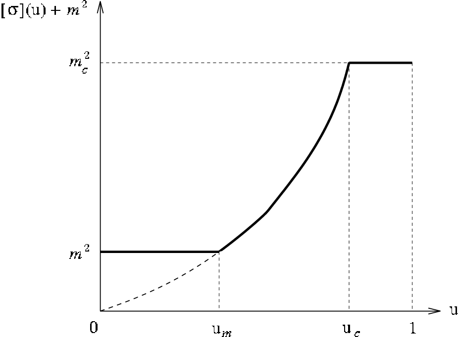
where , and was given in (20). As we will show later, this equation is only valid in the non-glassy regime since it was derived under the implicit assumption that the replica symmetry is not spontaneously broken as . Taking a derivative with respect to the mass and introducing a scaled function a FRG equation was derived for the renormalized and scaled potential correlator (denoted in Refs. LeDoussalWiese2001; LeDoussalWiese2003b). Remarkably, this FRG equation admits a natural continuation to the glassy regime. In that continuation a linear cusp exists for all . The resulting large- equation, valid to all orders in , exactly matches the equation previously derived to first order in (1 loop) but for arbitrary by Balents and Fisher BalentsDSFisher1993 by a quite different method. In addition, for all universality classes characterized by (,), such that (ensuring continuous RSB in the GVM), the fixed points could be related to the solution of the GVM. All the above strongly suggested that the derived flow equation was the correct large- limit of the FRG.
II.2.3 Relation between GVM and FRG in the case of continuous RSB
However, establishing a link between the GVM results and the FRG is rather subtle. To a considerable extent, this has been achieved for the case of continuous RSB in Refs. LeDoussalWiese2001; LeDoussalWiese2003b , while the same task for situations exhibiting 1-step RSB has remained an open problem, which is addressed in the present paper. In order to review the results for the continuous case, we recall the multiplication formulae for two ultrametric matrices :
| (36) | |||||
| (37) | |||||
| (38) |
where:
| (39) | |||||
| (40) |
We also introduce the notation for the diagonal element .
From (22) above one finds:
| (41) |
and from (14) we obtain
| (42) | |||
| (43) | |||
| (44) |
Further, using , we find:
| (45) |
(we often denote here and below) which relates to the self-energy , which for is given by (22) and (41).
In the GVM the 2-point correlation function is thus given by contributions from states at all distances as:
| (46) |
Using (41) and integrating over yields the final result:
| (47) |
in the limit , with and with , exhibiting the anticipated scaling.
On the other hand the FRG allows one to compute the two point function using (33) through the exact relation:
| (48) |
which, upon matrix inversion yields the zero-momentum correlation function:
| (49) |
It turns out that this does not yield the full MP result (46,47). Indeed, the contribution from the integral over in (46) is missing. However, Eq. (49) exactly reproduces the first two terms in (46), i.e., the contribution from the most distant states corresponding to , as well as the trivial term describing the connected correlations . Using the natural continuation to the glassy regime of the RG flow associated to the solution of (35), it was indeed inferred that
| (50) |
as will be derived rigorously in Section IV. This is already a non-trivial result: obtaining it within the GVM does require the RSB Ansatz, while the FRG considered in Refs. LeDoussalWiese2001; LeDoussalWiese2003b does not make reference to ultrametric matrices and their properties.
The fact that the FRG calculation of Refs. LeDoussalWiese2001; LeDoussalWiese2003b reproduced only the contribution of the most distant states within the Parisi hierarchy was argued to arise because and were computed by introducing sources which split all replicas, i.e., (and of order ) for all . However, it remained to be understood how the full result (47) can be recovered and how the crossover to spontaneous RSB takes place as .
This is the aim of the present paper. We will show the existence of a regime whose large- limit is different from (32):
| (51) |
and where RSB cannot be neglected. This will allow us to recover the complete GVM result, i.e., to correctly perform the (non-trivial) zero-field limit in (48). We first show, in the following section, that it is equivalent, but physically more transparent, to study the generating functional rather than . Further, we will revisit the attempt by Balents, Bouchaud, and Mézard BalentsBouchaudMezard1996 to connect RSB and FRG. Although we choose a different observable than those authors (so as to connect more directly to the FRG) we employ techniques similar to theirs, at least in the regime .
II.3 Observable studied here
The observable studied here is the free energy of the elastic manifold in a quadratic potential well centered at position , and defined by 1010 10 The definition of can alternatively be interpreted as the free energy of the elastic manifold (with elastic properties described by ), where the quenched disorder has been displaced by .:
| (52) | |||
with . For a uniform , one has 1111 11 As usual formulae for discrete sums are obtained replacing , and for a uniform one has .:
| (53) |
It is then clear from the definitions (29,52) that the statistics of can be obtained from the functional with:
| (54) |
Hence we denote , such that:
| (55) |
It is thus clear that the functional can be expanded in a cumulant expansion, i.e., in the number of replica sums:
| (56) | |||||
up to a constant, where again , etc. Each term in the expansion is a functional, with fixed , etc., and represents the free-energy cumulants:
| (57) |
and similarly for higher cumulants (the overbar denoting the disorder average over the random potential ). For a uniform configuration one has
| (58) |
which defines . Note that with arguments in brackets we denote functionals, while is reserved for functions. When discussing uniform we usually switch to the function , separating out the volume factor.
As shown in Refs. LeDoussal2006b; LeDoussalToBePublished by performing the Legendre transform (31), this observable is directly related to the function of the FRG:
| (59) |
i.e., the two functions are the same, and this holds for the functionals, too. Therefore, by computing , which we do here for large , we simultaneously compute as defined from the effective action (33). The fact that (57) defines an observable which is easy to measure has allowed for a numerical determinationMiddletonLeDoussalWiese2006 of or, more precisely, of the force correlator , for interfaces at .
The derivative of at contains information about the shocks. Indeed, if one computes the ground state for a fixed well position and defines the center of mass displacement , one finds that the latter exhibits jumps as is varied. The statistics of these jumps is encoded in the functions , etc., for instance one has:
| (60) |
and the cusp of , i.e. the derivative of at argument , is proportional to the second cumulant of the jump sizes.
We now turn to the calculation of this observable in the large- limit. We will perform separate calculations for the two scaling regimes and in the next Sections and check that they match.
III Regime of small ,
We want to compute the generating functional (29) in the form
| (61) |
This can be carried out at large through the saddle-point method as in Ref. MezardParisi1991, introducing the term and integrating over the field . This is detailed in the next Section where we study the case where which distorts the saddle point away from (14,15). In this section, we study and the above saddle points are unchanged (more precisely, they are shifted only by terms at most of order which are discarded). Since there is spontaneous RSB, there are in fact many saddle points equivalent under replica permutations. Hence the above average must be written as a sum over all equivalent saddle points:
| (62) |
where belongs to the group of permutation of replica which is used to label the saddle points. Around each saddle point the measure is Gaussian with correlator where is the ultrametric matrix given by (14). Hence we obtain:
| (63) |
where denotes a normalized average over permutations, i.e., . The remainder of this Section is devoted to the analysis of this formula.
In principle, by expanding this formula in powers of to all orders, and regrouping terms one could check that it is indeed possible to put it into the form (56), and to compute all the cumulants (we denote by the -th cumulant). This is a formidable task, however, and we will focus here only on the second cumulant function . Before computing it directly, let us give a flavor of the direct expansion in powers of .
III.1 Direct expansion in powers of
The expansion of (63) in powers of starts as:
| (64) | |||||
Let us recall the structure and parametrization of a hierarchical Parisi matrix. Dropping temporarily the -dependence one has footnoteRSB; footnote:order_of_u's
| (65) | |||||
| (66) | |||||
| (67) | |||||
We have defined as the matrix made of identical blocks along the diagonal, each block being the by matrix with all entries equal to one, and . As an example,
| (68) |
With these formulae one easily checks that
| (69) | |||||
For symmetry reasons, the permutation average must yield a replica symmetric matrix
| (70) |
Setting one finds , while multiplying with shows that . Thus, one finds:
| (71) | |||||
which is a replica symmetric matrix by construction, but with non-trivial entries in the case of RSB. Terms of higher order in have been neglected, except for the linear term in the replica diagonal part which we retain for later use.
Inserting in (64) we finally have
| (72) | |||
On the other hand, expanding (56) we obtain, for :
| (73) | |||||
since the fourth cumulant must start as and the third as (as one cannot construct STS invariant combinations of smaller degree - see Appendix B of Ref. BalentsLeDoussal2004 for an argument in the case ). Here and below we adopt the notation
| (74) | |||||
| (75) |
where the last line uses translational invariance and one has set after taking the derivatives. Further, we have assumed symmetry so that the second derivative of is diagonal and independent of the index in (74) (where no index summation is assumed).
Identifying (72) and (73) shows that for :
| (76) |
the second identity being a simple consequence of the STS symmetry. Hence, once the functional of the FRG is known, the correlation function computed via the GVM can be retrieved as:
| (77) |
This property of , here guaranteed by its definition (63) via the effective action, does not hold for the observable defined in Ref. BalentsBouchaudMezard1996 (having a similar form but with ). This made the comparison of their results with the FRG problematic.
To evaluate the identity (76) at , we use that for a uniform , , and thus:
| (78) |
which yields:
| (79) |
This relation is exact, and the task is hence to evaluate . There is however a crucial subtlety in evaluating this derivative at . If one uses that , together with the result of Refs. LeDoussalWiese2001; LeDoussalWiese2003b:
| (80) |
a relation also obtained directly in Section IV.2, one finds that (79) coincides with formula (49). However, this result is valid only in the region and, as pointed out above, it does not reproduce the full MP result for . To obtain the latter, as we show below, one needs to be more careful in the limit and compute in the region where . One could say that the and limit do not commute, or more accurately, that to obtain contributions of all ultrametric states (and not just the most distant ones) one must take the limit with great care.
The next order is obtained in App. B by the direct expansion method and in the next Section by a more powerful method which can handle all orders, and to which we now turn.
III.2 Second cumulant from a two-group analysis
While the results of the previous section were completely general and independent of the RSB scheme, we now focus on a specific choice of external sources. In order to compute the second cumulant function, one best uses two sets of replica, which we denote by for and for . Inserting into (56) we find
| (81) | |||||
where
| (82) |
since all higher cumulants yield higher powers of . We compare this with expression (63), slightly rewritten as:
| (83) | |||
In order to perform the sum over permutations, we introduce Ising spins as in Ref. BalentsBouchaudMezard1996:
| (84) |
where if , otherwise. Each configuration is left invariant by permutations, the number of distinct spin configurations being . They all correspond to vanishing total magnetization, i.e., . Inserting (84) into (83) the term linear in vanishes, and one finds:
| (85) |
The first factor equals the term proportional to in (81), as seen upon using (76). The prime on the sum indicates that the sum extends over all Ising spin configurations subject to the global constraint . Identifying the above expression with (81), we arrive at the formula:
| (86) | |||||
Note that we have simplified notations by renaming . At this stage we can check the small- expansion again:
| (87) | |||
If we denote the normalized average then one has . Further, the identity implies and one can thus write and . Using this in (87) we recover the result (76) of the previous Section. Note that the same result is obtained from the piece in the replica-diagonal part of (72), while the two-replica sum vanishes.
To evaluate the restricted spin sum in (86) we use the same method as in Ref. BouchaudMezardParisi, leading to Parisi’s nonlinear diffusion equation in the form discussed by Duplantier Duplantier1981. We first eliminate the constraint of zero magnetization and rewrite (86) as:
| (88) |
which makes use of an identity derived in Ref. BouchaudMezardParisi, valid for only.
The evaluation of a spin sum such as it appears in (88) is standard in the mean-field theory of spin glasses. Here we summarize the main steps following Duplantier Duplantier1981. We write the matrix which couples the spins as
| (89) |
with . Using (45) this becomes
| (90) |
Let us now assume that has a -step ultrametric structure with breakpoints at
| (91) |
and entries parametrized by with
| (92) |
Further we define . Let us introduce the “partial partition sums”:
| (93) | |||
which defines and for . Obviously, .
As shown in Ref. Duplantier1981, the functions satisfy a recursion relation, the idea being as follows. Consider one of the equivalent groups of size , for instance the first one . It contains subgroups of size footnote:order_of_u's. The only coupling between the subgroups is through the matrix with 1212 12 The term naturally arises in the construction footnoteRSB for a complete Parisi matrix, see also (67). Here it arises from the extra term in the definition of which involves an incomplete Parisi matrix, (the replica sum is interrupted at )., which couples uniformly all spins in the group. They can be decoupled by a Hubbard-Stratonovich transformation, adding a term , where is a Gaussian random field of variance , acting on all spins in the group. This allows to perform configurational sums independently within each subgroup and yields the recursion relation:
| (95) |
where here and below denotes the average over a unit Gaussian.
III.3 Continuous RSB: Second cumulant from an evolution equation
In the case of continuous RSB, we have to take the continuum limit in the above: , and , while . For the function , Eq. (95) yields a differential equation:
| (96) |
with initial condition:
| (97) |
where we assume to be constant for , as is generally the case, cf., (22).
Eq. (96) must be integrated from to , where reaches its lower plateau . If , the recursion (95) for shows that we have to perform a last convolution to obtain
| (98) |
The solution of (96) with initial condition (97) behaves at large like:
| (99) |
as can be seen by substituting (99) into (96). This is also confirmed by noting that for the sum in (88) is dominated by the configuration with all , which leads to the simple approximation (99) for . This behavior implies , since from the condition . Hence the integral (94) converges, the subleading terms of decaying exponentially at large .
We can now state the main result of this section. In the regime , the second cumulant functional can be obtained from the saddle point of the GVM as follows:
| (100) |
where the function is the solution of
| (101) | |||
| (102) |
in the interval , and
| (103) |
Eq. (100) follows from Eq. (94) by integration by parts, using that as discussed above.
From the above and (89) we see that the dependence of the functional on the field occurs only through the combination , where . Hence for a uniform one easily sees that and we can expect that (100) will assume a scaling form with scaling variable . This dependence on the system size is very different from the one in the regime and will be commented on further below.
The convolution (103) only results in an additive contribution to the potential correlator. This can be seen using the identity:
| (104) |
proven in App. C for functions whose derivative decreases faster than at infinity. Applying (III.3) to , we can rewrite (100) as:
| (105) | |||||
This result can also be derived via an alternative route, providing a useful check of the above formalism: In (88) we can directly separate out the contribution form the most distant states by writing , with , and . One can easily check that the piece produces the first term in (105). The remaining part leads to the same expression as (88), with the replacement . The only difference in the subsequent evaluation is that there is no need for a convolution in the end, since . This establishes (105).
Note that the first term in (105) has the expected form for the contribution from the plateau , cf., Eqs. (46,50), with a coefficient of
| (106) |
independent of . Clearly, this term is the only contribution in the case of a replica symmetric solution. We now show that it also gives the dominant contribution at large of order , but .
III.3.1 Limit of
In this case, Eq. (101) can be rewritten as
| (107) |
since is large (from now on we denote by a prime). One can integrate this equation to , where the integration constant (w.r.t. ) is fixed by the fact that for large , which cannot be changed by the evolution (101). The solution of (107) is then . One can check that the flow of is attracted to this simple “fixed point” as , if , with defined below. In that case, the second term in (105) becomes:
| (108) |
and the large- behavior of the second cumulant in this regime is thus:
| (109) |
The leading behavior is quadratic in and corresponds to the contribution of the most distant states to the full (inverse) correlation. Hence it should match the result obtained in the FRG for the regime , cf. Eqs. (49,50) or equivalently, Eqs. (79,80). Indeed, it does!
For a uniform and in the limit , one finds for both models (8,9), using (22,24):
| (110) |
This suggests a crossover around defined as:
| (111) |
The physical meaning of this crossover scale will be discussed in more detail in the context of the models with one-step RSB below, cf. Sec. III.5.
III.3.2 Perturbation expansion for
Since for , one has there is a uniquely defined expansion in powers of , which since is equivalent to the direct expansion in powers of of Sec. III.1:
| (112) |
Each contains only terms of degree . They satisfy the recursion:
| (113) |
where here and below dots denote . The initial conditions are . The final result for is:
| (114) | |||||
where we recall that . Hence contains all terms of degree , and we are thus effectively computing the derivatives at the origin, .
This calculation is performed in Appendix D, and the results are indeed consistent with the direct expansion of Sec. III.1 although the method is quite different. The lowest order term reads:
| (115) | |||||
using that , recovering the result (64,71) which yields, at small , the full result of Mézard-Parisi for the correlation function.
The next-order term is:
| (116) |
As discussed in Refs. NattermannScheidl2000; ChauveLeDoussal2001; BalentsLeDoussal2004; LeDoussal2006b; LeDoussalToBePublished the fourth derivative at zero of the FRG function is a direct measure of susceptibility fluctuations. Indeed we find that our present result has the general form of susceptibility fluctuations within a Parisi Ansatz, defined and derived in Ref. MezardParisi1991 .
III.3.3 Thermal boundary layer: General formula
It is possible to resum the derivatives, order by order in temperature and derive the thermal boundary layer (TBL) form:
| (117) | |||||
where the first term is the “zero-temperature limit” of the leading small- quadratic term 1313 13 When comparing (117) with (115), note that because of (79)., and the higher-order terms in the expansion in are scaling functions of the boundary-layer variable:
| (118) | |||||
| (119) |
This structure, which appears already in the 1-loop FRG, can be computed exactly in the large- limit here.
This structure appears already in the 1-loop FRG where one finds that at the non-analyticity of is thermally rounded. ChauveGiamarchiLeDoussal1998; ChauveGiamarchiLeDoussal2000; BalentsLeDoussal2004 Since temperature is irrelevant in the RG sense when this rounding occurs only in a layer determined by , which becomes smaller and smaller as , hence the name thermal boundary layer. Here, for the first time we compute its exact expression in the large- limit.
We now perform a (slightly more formal) expansion which allows to obtain (117). The idea, looking at (101), is that the nonlinear term contains an extra factor of and that for one has . Hence it is natural to expand in the nonlinearity to generate a low-temperature expansion. Of course this must be checked a posteriori. Further, we find it more convenient to use instead of to parameterize the ultrametric distance. Thus rewriting (101) as , and expanding formally in powers of , we have to solve the hierarchy:
| (120) | |||
| (121) | |||
| (122) |
Note that this hierarchy is formally similar to (113), apart from a shift in the index of the linear term on the RHS which indicates that we actually perform a different resummation.
The initial condition is , . Again, primes stand for . We define:
| (123) | |||||
| (124) | |||||
| (125) |
where we use the notation to distinguish from the expansion in powers of discussed in the previous Section, and different from the defined in (117).
The equation for is a simple diffusion equation with solution:
| (126) | |||||
| (127) |
Thanks to the identity (III.3), when from (126) is substituted into (124), we obtain
| (128) |
whereby the terms proportional to cancel. In the limit (128) becomes the same as the first term in (117), since:
| (129) | |||||
Here, we used and the fact that has a finite limit as .
To obtain the next order term, , we solve Eq. (121):
| (130) | |||||
where:
| (131) |
is the (reverse) diffusion kernel satisfying , and is the inverse function of for . Eq. (130) can be rewritten as:
| (132) | |||||
which inserted into (125) gives:
| (133) | |||||
We can now use the identity (III.3) for which has rapidly decreasing derivatives and satisfies . This yields:
Integrating by parts over and using the solution (126) for one finally obtains:
| (134) |
Note that we have used as primitive of , since we need it to vanish for large argument. Using
| (135) | |||||
we obtain the exact scaling functional for the thermal boundary layer 1414 14 Note that the function in (136) differs from in the systematic expansion (117) by a trivial quadratic term .:
| (136) | |||||
where:
| (138) |
has a finite limit as , where we introduced the definitions:
| (139) | |||||
| (140) | |||||
| (141) |
III.3.4 Thermal boundary layer: Uniform and scaling function for
Let us consider here a uniform for which one has:
| (142) |
Here and below we define:
| (143) |
One can rewrite with:
| (144) |
where here we denote and (not to be confused with the connected correlator ). Let us now specify to models I and II. One finds:
| (145) |
where was given in (25). Hence:
| (146) |
with , and . Using (146) we obtain the TBL function as a double integral in (144). In the limit this simplifies to:
| (147) | |||||
where is the scale obtained in (111). Further, from (25), depends only on and . The scaling function depends only on , while the argument is scaled by the characteristic displacement multiplied by the scaled temperature . This indicates that the scaling function of the thermal boundary layer exhibits universality for since only scales of order contribute to the final scaling function, all features of with being subdominant.
III.3.5 Non-analytic cusp from the limit of the TBL
The TBL functional (136) exhibits a non-trivial large-argument limit, (or, equivalently, ):
| (148) |
using that . This limit must match the limit of the functional , denoted . More precisely, as we will show in the next subsection, must match the cubic term of , i.e., the cusp non-analyticity.
We now perform an explicit calculation for a uniform . From (144) one finds in the limit of large :
| (149) | |||||
| (150) |
which produces a cusp non-analyticity at zero temperature. The coefficient can be computed explicitly for models I and II using Eq. (145,146) and one finds:
| (151) | |||||
One can check that in the limit , one has and that the prefactor agrees, using (149), with the one obtained from the large limit of (147). We have thus obtained the exact leading non-analyticity at zero temperature: it consists in a linear cusp in the force correlator, . This non-analyticity is of the same kind (i.e., proportional to ) as the one found in the standard FRG (e.g., to one loop for any ), and in the large FRG in the regime , which will be discussed in detail in the next Section. However, there are differences in the dependence of the amplitude of the cusp on , and . Anticipating the results of Sect. IV, they can be summarized as follows. In the regime one finds:
| (152) | |||
where , as well as are numerical prefactors (with ). Note that the two scales and are very different. The non-analytic corrections in the regime are related to the occurrence of shocks in the system, as the quadratic well is moved. Their contribution starts dominating once .
From (151) one finds that the amplitude of the cusp is zero at the Larkin mass , and then grows linearly as function of . This is in contrast to the large- regime, where the amplitude jumps to a finite value at , cf. Eq. (270) below.
Let us finally point out that a cusp non-analyticity proportional to in the regime was found in Ref. BalentsBouchaudMezard1996 , but with an amplitude scaling differently with . This resulted from a calculation of a rather different observable which is reviewed in Appendix E. A closely related cusp singularity was also found in the study of shocks in Burger’s turbulence. BouchaudMezardParisi (for a recent discussion of their relation to FRG see Ref. LeDoussal2006b).
It is important to note that the non-analyticity found here at in the regime is a robust feature that occurs irrespectively of the type of the ultrametric RSB scheme (whether continuous or 1-step, marginally or fully stable). As will be discussed below it reflects the switches in the minimum energy, and shock-like jumps in position, which occur as the energies of two states cross upon moving the harmonic well. It is, not surprisingly, rounded by temperature. In that sense it has some similarities with shocks discussed for interfaces , and for Burgers turbulence. In contrast, in Section IV the cusp in the regime will be seen to rely on the marginality of the RSB-scheme with respect to clustering fluctuations on the largest scales. That type of marginality only occurs naturally for systems exhibiting continuous RSB. As we will see, in that case a cusp occurs even at finite , in contrast to the above discussed non-analyticity which forms only in the limit . As we will discuss later, it is related to a more global transformation of the set of states as is varied.
III.3.6 limit of
The above described perturbation expansion is also perfectly suited to analyze the limit , where it turns into a rigorous expansion in . A similar expansion was pointed out in Ref. BalentsBouchaudMezard1996 . To exhibit the dependence on and , we define by introducing the reduced coupling function:
| (153) |
where in this paragraph we denote by a suitable average of , such as , such that is just a form factor. As mentioned before, and its inverse have finite limits, taking values between and , respectively. After rescaling , the evolution equation (101) for becomes:
| (154) | |||
| (155) |
and the second cumulant takes the form;
| (156) | |||||
From (154) it is easy to see that the above described procedure corresponds to a power series expansion in , the term corresponding to being proportional to . We will show below that in the case of a one step RSB the zero temperature correlator can be obtained in closed form.
III.3.7 Comparison with the TBL from droplet arguments
It is interesting to note certain analogies with formulae obtained from droplet arguments, where one assumes rare quasi-degeneracies of the ground state. In it was found in Refs. LeDoussal2006b; LeDoussalToBePublished that:
| (157) | |||
| (158) |
where is the difference between the center of mass displacement of the ground state () and of the excitation (). They are characterized by an (unnormalized) distribution where is the (normalized) joint distribution of position and energy differences between the two states. Here we denote , which can be normalized using the STS identity . In some simple cases (e.g., the Sinai model, corresponding to with random field disorder) is known analytically. The above formula can be generalized LeDoussal2006b; LeDoussalToBePublished to any :
| (159) | |||||
with , and a formula for all cumulants was also obtained.
Given the similarities between the formulae (157) and (136), it is tempting to interpret the latter in terms of a droplet size density, summed over all ultrametric distances . To this end, we rewrite (136) for uniform as:
| (160) |
where we note that and its inverse function are independent of .
As shown in App. F, the force correlator splits into a longitudinal and transverse part, describing forces parallel and orthogonal to the displacement vector . Note that due to the symmetry the correlator is only a function of . The TBL contribution to the force correlators is and , respectively. They can be cast in the form (for details see App. F):
| (161) |
with the densities
| (162) | |||
| (163) | |||
This has precisely the same form as the droplet expressions for the force correlators, which from (157) are found as:
| (164) | |||
where (for any fixed ), and the densities are given in (325). Note also that formulae (134,135), and the appearance of the function , bear similarities to expressions obtained in the case for averages over a uniform density of shocks rounded by temperature LeDoussal2006b; LeDoussalToBePublished.
In order to go further in the comparison and extract observables such as shock and droplet density and their size distribution, a more detailed description of higher moments is needed for the present model. Work in this direction is in progress.
III.4 The case of 1-step RSB (, )
As mentioned before, the GVM saddle point for a 1-step situation is characterized by the “break point” [ in the notation of (91)] and the two self-energy parameters (28). Similarly, the correlation function and the coupling assume only two off-diagonal values and . The former has the following interpretation: The measure on configuration space describing fluctuations both due to disorder and thermal noise can be constructed independently for each mode , following Ref. MezardParisi1991.
For the displacement in each environment one picks a set of “state centers” as 1515 15 Independently for each of the components . This is left implicit here in order not to burden the notations.
| (165) | |||
| (166) |
where the , are chosen from independent univariate Gaussian distributions. Note that in a given environment the (infinite) set of are globally displaced by the same (random) . Each state corresponds to a partial Gibbs measure which is assigned a weight (with ), such that the total Gibbs measure in this environment is the weighted superposition of the partial Gibbs measures, i.e., in one thermal realization one picks a state with probability and the mode takes the value
| (167) |
where are chosen from independent univariate Gaussian distributions and account for thermal noise inside a given state. In each environment the weights are independent random variables chosen from the distribution , the glass transition corresponding to the divergence of its first moment at large , which implies that only a few states dominate the total Gibbs measure. 1616 16 Equivalently, one can write with a tail for large negative . An analogous construction applies in the case of continuous RSB, where the obvious generalization of the above to -step RSB has to be taken to the limit .
With a general 1-step Ansatz of the form (14) we obtain the correlation functions:
| (168) | |||||
| (169) |
where As always, on the saddle point, STS implies , and we note:
| (170) |
With such a 1-step Ansatz the GVM free-energy density takes the form: MezardParisi1991
| (171) | |||||
| (172) | |||||
where we denote the square of transverse intra/inter-state fluctuations as:
| (173) |
and we have absorbed quantities that depend only on and , but not on and , into the constants and . The free-energy density (171) is minimized with respect to by the saddle point satisfying [Eq. (15)], taking the 1-step form:
| (174) |
In order to describe equilibrium thermodynamics, the breakpoint has to be chosen so as to extremize (maximize) , as usual in replica treatments. However, other choices of are of physical interest as well, as discussed in detail below.
III.4.1 Instability of the RS solution
Let us derive the phase diagram in the 1-step case. For simplicity we restrict to and . We recall that we use the natural units introduced in Section II. Performing the integrals, the free-energy density reads (dropping the constant ):
| (175) | |||||
where we have used
| (176) |
In (a particle) the last line of (175) becomes . In above, and can be considered as two independent variational parameters. The variation with respect to (at fixed ) yields back the saddle-point equation:
| (177) |
where from (173) one has:
| (178) |
The replica-symmetric solution (, , ) is valid at high temperature/large mass, but becomes unstable when the condition
| (179) |
is met, with . This defines a unique function for masses smaller than the zero temperature critical mass: 1717 17 We make the natural assumption that is monotonously decreasing with .
| (180) |
The function describes the location of a continuous glass transition towards a 1-step RSB phase for . Here, denotes the mass where attains its maximum. For , the line has little physical significance, since in that regime the glass transition occurs in a discontinuous manner at , as will be discussed below.
It is interesting to note MezardParisi1991 from (165-167), using (168-170), that as the thermal fluctuations of the displacement field within a state, remain bounded and massive and occur only at the Larkin scale.
By contrast, the r.m.s. difference in displacement between two states in a given sample, , scales as . Hence, the thermal fluctuations between states, which are active at any in a given sample, occur at all scales up to . Note that these r.m.s. differences in displacement have a finite limit, if goes to a constant in that limit (which is generally the case as shown below). These fluctuations are responsible for the roughness of the manifold with a non-zero amplitude even as .
Finally, sample-to-sample fluctuations include in addition the term whose mass dependence is controlled by . These fluctuations also occur at all scales smaller than .
III.4.2 Metastable states and configurational entropy
The break point is a priori a free parameter of the 1-step Ansatz. In order to describe the thermodynamic equilibrium, one should choose which extremizes the free energy:
| (181) |
(at fixed ) as was done in Ref. MezardParisi1991. As in most glassy problems with a 1-step structure, at low temperatures the equilibrium break point is proportional to the temperature 1818 18 We correct a misprint of the 1-step solution given in Ref. MezardParisi1991 , which suggested that . . This is shown in App. G, where is computed as well.
However, the function encodes much more information than just the equilibrium physics. It can be interpreted Monasson95 as the quenched “replicated free energy”, i.e., the free-energy density per replica of a set of clones (replica) which are bound to remain in the same metastable state of the energy landscape. With this interpretation one can alternatively write the total free energy as a sum over states. Their number at fixed free-energy density increases exponentially with the volume and . One thus introduces the configurational entropy, or complexity, . The total Boltzmann weight of clones can then be written as:
| (182) | |||
where . In the large- limit, the configurational entropy becomes the Legendre transform of the replicated free energy:
| (183) |
Knowing , one easily obtains an implicit parametrization of the configurational entropy as a function of the free-energy density:
| (184) | |||||
| (185) |
We see in particular that the equilibrium prescription (181) corresponds to choosing the states with vanishing configurational entropy. Since the configurational entropy is an increasing function of , the so selected states have the lowest free-energy density in typical samples and thus describe indeed the quenched equilibrium free energy.
However, the equilibrium may not be possible to reach dynamically, which suggests a different choice for . The choice is constrained by the requirement that the 1-step solution be stable (as was the case for ).
Metastable states of the free-energy density above the equilibrium value are described by breakpoints in the range , where the lower boundary is determined by the so-called replicon instability of the 1-step scheme, i.e., the condition: footnoteinstability
| (186) |
A comparison with (179) shows that at fixed temperature , this implies , where is uniquely defined as the solution of . One can prove that solutions of the 1-step saddle-point equations with condition (186) exist for all and (but nowhere outside this parameter regime). 1919 19 However, will exceed 1 at small and close enough to . The states described by are merely marginally stable and are often referred to as “threshold states”. Since they are usually the most abundant metastable states of the system they are most likely to trap the dynamics after a fast temperature quench for .
Another choice for of interest is the value where the 1-step scheme becomes unstable with respect to a clustering fluctuation among the existing states footnoteinstability. The latter is equivalent to the condition:
| (187) |
This condition ensures that the second cumulant in the regime is non-analytic at , as we will discuss in Sec. IV.2.4.
We emphasize that the kind of marginal stability imposed by (187) is clearly distinct from the marginality (186) due to the replicon mode, which is usually imposed to select dynamical threshold states in 1-step systems 2020 20 Even though distinct they may occur at the same value of parameters in the case of the marginal one step solution.. The latter is also the marginality property of continuous RSB systems that ensures the presence of collective soft modes in classical BrayMoore79 and quantum mean-field spin, elastic or electron glasses CugliandoloGiamarchiLeDoussal2006; GiamarchiLeDoussal1996b; Schehr2005; MuellerIoffe07, and leads to a universal, saturated pseudogap in the local field distribution of spin and electron glasses MuellerIoffe04; Pankov06; MuellerPankov07.
While the replicon instability (186) indicates the fragility towards fragmentation of existing states into substates, the condition (187) signals the instability towards the formation of clusters among previously equivalent states. When these two instabilities involve rather different length scales. This can be seen as follows: The replicon instability corresponds to each state in (165) giving birth to a new cluster of substates labelled by , , where each occurs with a probability (with ). This rearrangment implied by the additional substructure involves scales of order since with . On the contrary (187) signals the instability towards splitting into several clusters , generating substates . This rearranges the original into clusters labelled by , and obviously involves scales up to .
The above two kinds of instabilities have been analyzed in detail in the context of the spherical p-spin model in Ref. CrisantiSommers1992. More recently they have been discussed in the context of lattice-glass models Rivoire03 and optimization problems MontanariRicci-TersenghiParisi; KrzakalaPagnaniWeigt; ZdeborovaKrzakala07, where they are sometimes referred to as instabilities of the first (clustering) and second (fragmentation) kind 2121 21 In the case of lattice glasses one finds the same regions of stability for as here: The 1-step solution is unstable to replicon fluctuations for , while it is unstable to the clustering instability for .. They also appear as the instabilities driving the transitions between the two types of one-step phases adjacent to an intermediate two-step RSB phase in certain mixed spherical spin models. CrisantiLeuzzi07
For model I in , i.e., the directed polymer problem, we have checked explicitly that , and we expect this to be generally true for 1-step solutions. This is illustrated in Fig. 5. For the associated configurational entropies this implies , and thus the states selected by the clustering instability (187) have negative configurational entropy. Anticipating the analysis of Sec. IV.2.4, we conclude that samples exhibiting non-analytic shock-like behavior in the regime where an FRG equation was previously derived, correspond to exponentially rare realizations of the disorder occurring with probability , as derived explicitly in App. G.
Note that upon approaching the limit of a marginal one-step solution, i.e., for and , the three values merge and the one-step saddle point becomes simultaneously marginal with respect to both instabilities discussed above.
III.4.3 Phase diagram

In this section we establish the phase diagram and discuss some of the subtleties associated with the choice of . The situation is closely analogous to a particle in a random environment () analyzed in Ref. CugliandoloPLD. The phase diagram of a typical case, model I in , is shown in Fig. 4, and explicit values given in the analysis below refer to this specific case.

The glass phase exhibits everywhere 1-step RSB. Right on the instability line where (179) is obeyed, there is only one admissible value for :
| (188) | |||||
which yields the fluctuation-dissipation ratio relating response and correlations at the glass transition. CugliandoloPLD It increases monotonously with decreasing , and reaches at (, with in for model I where ). For states to be dynamically or thermodynamically of significance, must always be smaller than , and thus the line looses its significance below .
For the glass transition is continuous in the sense that smoothly goes to as . For the temperature-driven transition is discontinuous with a sudden jump between intervalley and intravalley correlations occurring at some . The location of the transition depends on the point of view. From a thermodynamic (static) standpoint the glass transition takes place at the line given by , indicating that the replica symmetry must be broken spontaneously to extremize the free energy, which gives rise to a non-analyticity in the free energy. For model I, one finds the explicit result
| (189) |
However, metastable states exist already at higher temperature. In the mean-field limit they induce a dynamical freezing transition at the line defined by . For model I one finds
| (190) |
The resulting phase diagram is naturally very similar to the one for a particle in a random environment (the limit of a random manifold) CugliandoloPLD, and it also strongly resembles the one of the spherical -spin model, whereby the mass takes the role of the external field CrisantiSommers1992. In the latter the glass phase is known to be everywhere of 1-step nature, the transition (at fixed ) being continuous for and discontinuous for .
III.4.4 Second cumulant
To evaluate the second cumulant of the renormalized disorder potential , we introduce as before the coupling , connected to via:
| (191) |
We need to apply the recursion relations (95) only once (since here ) to calculate:
| (192) | |||||
and using similar steps as in the derivation of (88) and (105) we obtain:
| (193) | |||
Recalling that , one can see that at large , and thus the integral in (193) indeed converges. In the following we examine various limits of this formula.
III.4.5 Large
Let us introduce the notation . At large (large ) one can use that , as can be shown using a saddle-point method. This yields the large- limit:
| (194) | |||
Evaluating the integral we find the final result:
| (195) |
which matches the full RSB result (109), if we formally replace by . These two expressions are indeed identical in the case of a marginal 1-step solution, as it occurs in . In that case, , and the analysis of the crossover to large in Section (III.3.1) remains unchanged.
III.4.6 Small
For small one can expand in as follows:
| (196) | |||
where was used. Performing the -integrals, one eventually finds:
| (197) | |||
As it must be, the leading term is:
| (198) |
which yields the GVM result for two-point correlations. Indeed, (198) matches the expression (115), which should not depend on the RSB scheme. Similarly, inserting the one-step form for in (116) one checks that it reproduces the second-order term from (197). In fact, one can check that (197,116) agree with:
| (199) | |||
where we have used and defined . Note that , where the dot is the Hadamard-product.
III.4.7 Low- expansion
Let us now consider the low expansion, i.e., the thermal boundary layer, using similar notations as in (III.3.3). In the limit , but has a non-zero limit, and so do and when expressed in terms of fixed , as in (118). Hence it is convenient to define, for the present 1-step case, an expansion in 2222 22 As in Sec. III.3.3, it does not exactly coincide with the expansion in powers of since some extra (weak) dependence is hidden in other parameters such as, e.g., . However, as before the series can easily be rearranged later., analogous to (123):
| (200) |
obtained by expanding (196) in powers of at fixed . This yields:
| (201) | |||
| (202) | |||
| (203) | |||
The expression for has been simplified using an integration by parts and the identity (III.3), and is found to match the result (128) for the continuous case. The term has been included in . The term multiplied by in(203) is the connected average (cumulant), as indicated by the superscript . After a calculation summarized in App. H we finally obtain the thermal boundary layer:
| (204) |
which agrees with the result for continuous RSB (136) as expected, since both formulae should apply for the borderline case of a marginal 1-step solution.
III.4.8 Cusp and full correlator at
The case of one-step RSB is sufficiently simple to allow for a complete calculation of the non-analytic limit of the full functional in the regime . Let us define the variable:
| (205) |
which will be shown to be of order when the crossover to the shock-dominated regime occurs, see (216) below. It tends to a finite limit as . For a uniform this becomes:
| (206) | |||||
with as given by (168,169). Note that the characteristic scale for (determined by ) is not exactly the scale for shocks found for continuous RSB in (111), but rather (for ) . However, the two scales become the same in the case of marginal one step RSB since there .
Let us first obtain the cusp for a uniform by taking the limit of large of the thermal boundary layer. In that limit the expression (204) tends to 2323 23 Agreement with (149) and (151) can be checked for the marginal one step case using , from (25), and .
| (207) |
using . This finite non-zero limit as (cf., App. G) is thus the exact expression for the leading non-analyticity of at , which is again cubic (corresponding to a “linear cusp” of the force correlator ). Note that in this regime, , the cusp exists irrespective of the choice of , including the equilibrium solution. This is to be contrasted to the regime where, in the case of a non-marginal one-step solution, a cusp exists only for the choice , see the discussion in Sec. IV.2.4.
We now obtain the full functional for arbitrary , using the variable defined in (205). By using (192) in (193) and taking the limit of small , we find at :
| (208) | |||||
where:
From the expansion for we again recover (207) with, in the uniform- case . The asymptotics for is in agreement with the result (195) for continuous RSB (with ).
From this expression one can compute the force correlator, which, from symmetry, splits in transverse and longitudinal parts as defined in App. F.
The non-analytic parts of the longitudinal and transverse force correlators in the regime are proportional to and , respectively¿ They are plotted in Fig. 6, both exhibiting a linear cusp at the origin. Note that the full correlator of the force in addition contains a constant which derives from the term in (208). Further decay from this constant to zero at infinity occurs (for any ) in the regime .

III.5 Interpretation of and the thermal boundary layer
What happens to the manifold as the center of the harmonic well is moved? Let us first focus on the case of a one step RSB for which the construction of the statistical measure is significantly simpler and was recalled in (165,166). From this construction we know that at low temperatures a certain state center dominates, but there is at least one excited state which differs in energy by a typical amount . Changing the position of the harmonic well by an amount shifts the relative energies of these two low lying configurations (states), noted , by an amount:
| (212) |
One can expect a switch from one state to the other, and thus a macroscopic jump, as the energies of two states cross. This occurs typically when . Recalling that is of the order of , one finds:
| (213) |
Hence, comparing with Eq. (205) the jump occurs typically when:
| (214) |
We thus understand the scale of variation of the functional given by (208,III.4.8). The argument is even simpler for a uniform center () which couples only to the mode of the excitation, the energy shift being . Since , we see that the energy shift (212) competes with the typical excitation energy when is of the order of as defined below Eq. (206). Since the energy difference is finite, the jump is thermally smoothed at finite temperature, but turns into a sharp shock for , which is at the root of the non-analyticity in (III.4.8).
We can obtain better insight into the physics for shifts of order by examining the force-correlator. We consider uniform for simplicity. To be specific we define which corresponds to the longitudinal force correlator. From (208), we see that for the correlator is simply constant and equal to:
| (215) |
This has a simple interpretation in terms of the hierarchical construction (165,166): One can imagine the states (characterized by ) as parabolic potential valleys within a big parabolic potential valley as determined by the global center , and accordingly write schematically for the total potential. For , the manifold has jumped to a different state center, and therefore the part of the force arising from does not contribute to the correlator. However, is very robust under shifts of , and jumps only once , as we will see in the next section. The force corresponding to the big valley, , thus remains constant. Since the disorder potential competes against the quadratic well , that part of the force is of order , which leads to (215).
For we see from (207) that the force correlator behaves as
| (216) | |||
The first term can be understood as times the intra-state correlator . The force correlations rapidly decrease with growing . Indeed, we can understand the non-analytic piece as being due to shocks which occur with a finite density along the -axis. Note the large prefactor of : It indicates that the product of the density and size of shocks scales as , that is, in such a way that the system size rather than acts as a cutoff. Further work is in progress to clarify the properties and the distribution of these shocks.
Let us close the discussion of shocks by sketching the analysis in the case of continuous RSB. The typical scale in that case, , can be retrieved by the same argument as above for the one-step RSB. However, now the energy difference between two states at ultrametric distance is typically of order . This competes with the energy shift induced by the displacement of the well:
| (217) | |||||
The largest response is due to transitions between states differing at the largest scales, i.e., . The above energy comparison at this scale immediately yields . However, there is no sharp selection of shocks that involve the highest hierarchy scale. Smaller shocks contribute as well, even though their weight decreases with increasing characterizing the shock. Note that from the construction of the measure of pure states it is clear that when a shock occurs at scale (in a finite -step RSB scheme), the whole sub-hierarchy of state-centers with changes. Note that in general shocks characterized by a larger correspond to smaller spatial rearrangements.
IV Regime
We now compute the functional defined in Section II.3, and more explicitly its second cumulant part , in the regime . This is the standard regime for the large- analysis, and in Refs. LeDoussalWiese2001; LeDoussalWiese2003b the associated saddle-point equation was obtained. There the focus was on the calculation of the effective action , and in particular its two-replica component , part of which will be of use here, too, to obtain and . We find, as announced in Section II.3, that the functionals and are identical. The calculations carried out here are, however, rather different in spirit from the one in Refs. LeDoussalWiese2001; LeDoussalWiese2003b . We obtain from imposing external fields to two groups of replicas, whereas in Refs. LeDoussalWiese2001; LeDoussalWiese2003b the case of for all was considered. It is reassuring that the two approaches yield consistent results. The advantage of the present approach is that it includes RSB effects, and hence it provides a complete derivation of the FRG equation on all length scales (below and above the Larkin scale).
IV.1 General saddle point
To analyze the saddle point in the regime it is convenient to introduce the rescaled variables:
| (218) |
We can now rewrite the definition (61) and decouple the partition sum with the help of two auxiliary fields as:
| (219) | |||||
where the replica matrix field has been introduced through a purely imaginary Lagrange multiplier matrix . A standard choice, as in previous sections, is but our analysis is more general. We have also included the source term shifting the center of mass. is a function of a replica matrix 2424 24 Note that . :
| (220) | |||||
containing the information about the bare disorder via its cumulants, e.g., its second cumulant being (as in (7)):
| (221) |
Note that the rescaling (218) was performed in order to make explicitly appear a factor of in front of the action , which allows for a saddle-point analysis. One now explicitly performs the functional integration over the field to obtain:
| (222) | |||||
| (223) | |||||
where the inversions and the trace are performed in both replica and spatial-coordinate space. We use the shorthand , which is diagonal in replica space.
Eq. (222) has now the standard form for a saddle-point evaluation of the functional except that the saddle point is not, in general, uniform in space. At dominant order in , we obtain
| (224) |
We have allowed for different saddle-points (“sp”) to contribute. To alleviate notations, we did not add an index indicating the different saddle-points to and . They depend on and are the solutions of the saddle-point equations obtained, respectively, by setting to zero the functional derivatives (at fixed ):
| (225) | |||||
| (226) |
Solving these equations, one can obtain from its definition (56).
The explicit form of the saddle-point equations is:
| (227) | |||||
| (228) | |||||
| (229) |
where is a matrix with both replica indices and spatial coordinates; thus inversion is carried out for both. The notation for the -component vector is a shorthand for a matrix product, but consistent with our above conventions, we do not write the vector indices of explicitly. We have defined the average displacement induced by the source:
| (230) |
It is a function of and of the chosen saddle point “sp” and to simplify notations we drop in what follows the dependence on except when an ambiguity arises. As detailed in Refs. LeDoussalWiese2001; LeDoussalWiese2003b , arises in performing the Legendre transform to obtain from , as one may see from (31) and (54), i.e.:
| (231) | |||
| (232) |
and using that for a given saddle point:
| (233) |
Taking the total derivative w.r.t , which is equivalent to differentiating only the explicit dependence in (225), one recovers (230). While in Refs. LeDoussalWiese2001; LeDoussalWiese2003b we had chosen sources such that and therefore assumed a unique saddle point, here we allow for spontaneous RSB and hence for many saddle points. In general the set of saddle points will include the set of all permutations which leave invariant 2525 25 Note that the condition is on and not on since the saddle-point equations are expressed in terms of . In other words, the condition is ., i.e., for all . Hence the in (230) is identical to a partial average (corresponding to a single saddle point labelled by ) while the thermodynamic average corresponds to the full average over all equivalent saddle points, . In the limit the saddle point equations (227) become identical to the saddle-point equations of the GVM, with and taking the values of the solution given by Mézard-Parisi (see also below). Performing the sum over equivalent saddle points in (224) one recovers the results of Section III.
IV.2 Analysis for a uniform
According to the general strategy to compute , as described in Section III.3, we now solve the saddle-point equations (225) and (226), specifying the source with entries , and entries . For simplicity we restrict here to a uniform , for which . From the definition (56) and the replica-sum expansion (81) one has:
| (234) |
up to a (-independent) constant. The matrices and are now independent of , and is translationally invariant. We parametrize the replica matrix by:
| (235) |
where we anticipate that the diagonal blocks will turn out to be independent of . We use similar notations for and :
| (236) |
Note that and should not be confused with the variables used for the 1-step solution. The saddle-point equations (227)-(229) now become:
| (237) | |||||
| (238) | |||||
| (242) |
and must be solved for a given value of . We have introduced the notation and for the matrices:
| (243) |
In general, we expect that is an ultrametric matrix while , and similarly for and . This Ansatz for the solution is motivated by the expectation that states in different groups will be very distant in phase space (at least as distant as the farthest equilibrium states, as described by ), and thus their mutual overlap will not depend on the specific replica in either of the groups. Further, we have , and one can show that our Ansatz implies
| (244) |
which means that the average displacement is tied to the center of the harmonic well. This holds because (230) implies , where (the sum being restricted to the replica in the same group as ) and (the sum being restricted to the replica in the group not containing ). Within our Ansatz, as , and vanishes (see (249) below), which establishes (244).
To evaluate (242), let us split the set of indices into two groups, for the first replicas, i.e. those for which , and for the remaining replicas, and consider for simplicity a bare model with gaussian disorder 2626 26 One may also consider higher bare cumulants . While both the saddle-point equation in the regime and the self-consistent equation for the correlator are changed, the essential results about the connection between the FRG regime and the RSB regime remain the same: One can derive a closed self-consistency equation for the renormalized force correlator (involving the bare cumulants ), from which the exact FRG equation can be derived; in the glass phase RSB introduces an anomaly in the selfconsistency and the FRG equation; the identity matching FRG and RSB regime holds everywhere in the phase diagram; the force correlator exhibits a cusp at the origin, if and only if the saddle-point solution is marginally stable with respect to clustering fluctuations.:
| (245) | |||||
One can easily see that Eqs. (242,245) imply the STS property . Applying the inversion formulae (36-38) to (IV.2), we find the exact relation (to all orders of ) from the connected part (IV.2). Further, to lowest order in one finds [cf., (42,43)]:
| (246) | |||||
| (247) | |||||
| (248) |
and, to precision :
| (249) | |||||
Up to negligible corrections of order the saddle-point equations for the diagonal blocks are the same as those in the regime , cf., (14,15), independently of the external field :
for in the group. An analogous equation holds for the diagonal block. This is not surprising since the external field does not separate the replica within a group. Since these saddle-point equations have a unique physical solution, we will identify henceforth, and also drop the subscripts on and . In Parisi’s parametrization of ultrametric matrices, the saddle-point equation is conveniently rewritten as
| (250) | |||||
| (251) |
The saddle-point equation for the off-diagonal part is:
| (252) |
which within our Ansatz reduces to a single equation
| (253) |
Before analyzing these equations let us indicate how to extract from its solution. Let us first rewrite the part of the action at the saddle point which depends explicitly on (in fact, on ):
| (254) | |||||
Since the derivative of , w.r.t. (in fact, w.r.t. ) only involves the explicit part we find, and comparing with (IV.2):
| (255) |
We now discuss various cases according to whether or not the replica symmetry is broken in the diagonal block, (the saddle point of the GVM), indicating whether or not the system is in a glass phase.
IV.2.1 Replica-symmetric region
IV.2.2 Identification with FRG below the Larkin scale:
It is convenient to introduce the function via the change of variables:
| (260) |
Plugging it into (253), we see that it satisfies exactly the self-consistency equation (35):
| (261) |
as derived in Ref. LeDoussalWiese2003b for the second cumulant function of which occurs in the effective action (defined there via ). Since (261) uniquely specifies up to a constant, a comparison of (260) and (255) shows that
| (262) |
i.e., we have recovered, in the glassy regime, the general identity announced in (59,80).
From the self-consistency equation (261) a FRG equation for can be derived, following [cf., Eqs. (6.1)-(6.8)] in Ref. LeDoussalWiese2003b
| (263) | |||||
with initial condition for .
At this stage we only know that the FRG equation (263) is valid in the replica symmetric region, i.e., for (see discussion in Section II.2). At the Larkin mass, diverges, signaling a cusp in the force correlator, as can be seen from the condition (19) and (261). Hence at the equation (263) is still valid, but the second term (involving the temperature explicitly) is negligibly small there and can be dropped. It is now crucial to establish how to continue this equation below the Larkin mass. To this end we compute explicitly beyond the Larkin mass, i.e., in the glassy region, where RSB occurs within the replica groups, and derive the correct FRG equation for .
IV.2.3 Self-consistency equation for the second cumulant below the Larkin mass
The saddle-point equation (253) together with (255) yields the correct continuation of the self-consistency equation (261) below the Larkin mass:
| (264) |
We expect that:
| (265) |
remains valid when replica symmetry is broken (with of course a different and non-trivial value for ) since it expresses the equality between the self-energy associated with distant equilibrium states, and that associated with the coupling among the two replica groups in the limit of zero forcing, . Indeed, one can check using (247) that (265) is a solution of (264), given that (250) holds. Note that (265) insures that the function perfectly matches the large limit of the results (109,195), irrespective of the scheme of RSB, as it should.
IV.2.4 Correlator and FRG equation below the Larkin mass
From (266) we easily obtain the behavior of the force correlator, , at small argument. If the RSB solution is marginally stable with respect to a clustering instability at the largest scales, i.e., if the condition
| (269) |
holds, with defined in (267), one finds a non-analytic cusp in the correlator:
| (270) |
This type of marginality is automatically ensured in the case of continuous RSB, which is marginal with respect to fluctuations on all scales (see App. I) including those corresponding to , which entails (269). For a 1-step solution, however, it occurs naturally only on the transition line for , while in the glass phase it requires the specific choice , cf. (187). In the case of a non-marginal 1-step solution, the latter choice differs from the value of corresponding to thermodynamic equilibrium, and was shown to describe rare disorder configurations in Section III.4.2. On the other hand, for a fully stable saddle point with , one finds the regular correlator:
| (271) |
We emphasize the difference between these results and the generic non-analyticity (149,207) found in the regime at , occurring irrespectively of the RSB scheme. The cusp in the regime analyzed here is present even at finite temperature, provided the RSB scheme is marginally stable in the sense of condition (269). The non-analyticity thus reflects the criticality of the system being at the brink of an instability towards an additional clustering of the topmost level of an ultrametric structure. In the 1-step case, the instability is towards a two-step RSB with an additional step in the lower plateau CrisantiSommers1992; CrisantiLeuzzi07.
Taking a derivative of (264) with respect to and using it to simplify (263), one finds LeDoussalWiese2003b repeating the steps of Eqs. (6.4)-(6.6) in Ref. LeDoussalWiese2003b:
| (272) | |||||
where
| (273) | |||||
This equation is the general FRG equation valid in all regimes. In the non-glassy RS regime and the amplitude is identical to the last term in (263). In the glassy region Eq. (272) is certainly valid for all , and it is also valid at if , i.e., if the RSB solution is not marginal in the sense of (269). But even if the solution is marginal, and hence is infinite (i.e., exhibits a cusp), both sides of the equation have a non-trivial limit at which yields another valid equation as can be checked using (270). Another useful expression for is obtained by rewriting the second equation in formula (273) as:
| (274) |
where we used the definition (267) and (268). The second term in (274) can be rewritten using the saddle-point equation (250) at , and taking a derivative w.r.t. one obtains
| (275) |
a formula valid in all cases and regimes. We already point out and will discuss further below that the amplitude vanishes if the marginality condition (269) is met.
Let us now analyze in more detail the case of continuous RSB which includes as a limiting case the marginal 1-step case occurring in with . In Ref. LeDoussalWiese2003b it was found that the consistent FRG equation 2727 27 For , but this should be the same as for . for was (272) without the last term, i.e., . As we discussed above, this matches the established equation (35) at . The validity of (272) for was inferred from the study of the FRG equation in inverted variables , noting that for models I and II the FRG flow completely stops at (the beta function is identically zero hence its natural continuation is to remain zero below ). In Section VIII-D of Ref. LeDoussalWiese2003b the analysis of the FRG flow was extended to an arbitrary bare model (i.e., an arbitrary ). It was found that the natural continuation is such that the function retains a cusp for all . This was found to coincide with the marginality condition at , and hence lead to (269,270).
From the above general expression (275) we see that the vanishing of the amplitude is a direct consequence of the marginality of the continuous RSB at , i.e., condition (269), and thus confirms the correctness of the assumption made in Ref. LeDoussalWiese2003b. In addition we discover here that the cusp can be avoided if there is a non-zero amplitude . This possibility was naturally not considered in Ref. LeDoussalWiese2003b, where the analysis was based on the self-consistency equation without anomaly and the ensuing FRG equation. While the amplitude always vanishes in the case of continuous RSB, a zero amplitude requires a specific choice of the breakpoint in the case of 1-step RSB, as discussed in the next Section.
IV.3 Discussion of the FRG flow
IV.3.1 General considerations
Let us analyze the generalized self-consistency Eq. (266) for the renormalized correlator function . It depends only on the (given) bare disorder function, and a number, , defined in (267). This is the only input from the saddle-point solution in the regime , which introduces an anomaly in the glass phase. We emphasize again that in the case of one-step RSB, does not only depend on and , but also on the choice of the breakpoint .
Since the force correlator (the derivative of the potential correlator) scales like , with typical values of the argument scaling as , it is natural to define the rescaled force correlator (as in Refs. LeDoussalWiese2001; LeDoussalWiese2003b ):
| (276) |
At this stage, if we ignore all other information from the regime, the two exponents and are undetermined. Let us assume for now that they can be fixed by requiring that reaches a non-trivial fixed point. From (266) one deduces that satisfies the equation:
| (277) |
where we have used in the limit of infinite cut-off, and consequently set , as expected, so that the last two terms in the argument of (the bare disorder) scale the same way. The only information needed from the regime is the value of , given by the saddle-point solution. It fixes the value of at the origin:
| (278) |
The above two equations then completely determine the FRG flow of , describing the evolution of the force correlator as the mass is decreased. The corresponding flow equation was given in (272). Here we directly solve (277) focusing on models I and II, which admit simple solutions. We distinguish the case of continuous RSB (full or marginal one-step), which we only briefly recall since it was discussed in detail in Ref. LeDoussalWiese2003b, and non-marginal one-step RSB which requires a novel and thorough analysis. The difference between the two cases can be grasped immediately. For continuous RSB, comparing (278) and (27), valid in that case for models I and II, we immediately see that reaches a fixed-point value with the same choice of exponents as in the regime. By contrast (173) and (177) suggest a rapid decrease of as as discussed below.
Some features are independent of the RSB scheme and worth mentioning. Consider model I, . If one makes the choice , then is the solution of
| (279) |
which has clearly a fixed-point form provided , given by
| (280) |
reaches a fixed point as . Similarly for model II, , and (278) together with the choice leads to the equation:
| (281) |
Upon inversion this allows us to simplify the equation (277) for the rescaled force correlator as:
| (282) |
which reaches a fixed point if does. Note that these expressions, as well as (277), are valid for all , both above and below the Larkin mass.
IV.3.2 FRG flow for continuous RSB
As discussed in Ref. LeDoussalWiese2003b for model I and II the flow is particularly simple. The structure of (279) and (282) imply that is always given by the same master function , shifted by an amount which depends on only through . For model I the master function is the solution of . The shift must be positive, and leads to a cusp (infinite slope) at the origin. In the case of continuous RSB freezes to zero as decreases below . One checks that reaches its fixed point value at :
| (283) | |||||
and remains constant everywhere in the glass phase. This implies in particular that reaches its fixed point already at the phase transition and sticks to it for all smaller , a result inferred in Refs. LeDoussalWiese2001; LeDoussalWiese2003b from the vanishing of the beta-function at . The FRG flow for models with continuous RSB is illustrated in Fig. 7.

As shown in Ref. LeDoussalWiese2003b for models different from I and II, and such that there is continuous RSB for all , such as linear combinations of I and II with various powers, the flow is slightly more involved. For the flow is not a simple translation in but the shape also changes as irrelevant parts of decay. At a cusp appears and remains for all as (and the shape of the function) converges slowly towards one of the above fixed-point values (283).
In the continuous RSB case, the existence of this family of non-analytic fixed points is related to the vanishing of the amplitude in the FRG equation. In Ref. LeDoussalWiese2003b they were derived directly from (272) assuming . For and , , they lead to the same exponents and as the study of the GVM regime, cf. Ref. MezardParisi1991 . Hence, all parts of the effective action scale consistently. Note that in the limit case , , the glass phase is described by a marginal one-step RSB solution. As discussed in details in Ref. LeDoussalWiese2003b (Section VI.D and Appendix F), the high-temperature phase is described by a line of analytic fixed points which solve (277) with , . In that phase converges to one of these fixed points. This line of fixed points terminates on a cuspy fixed point, towards which converge for , and which has the form (282, 283) with .
By contrast, in the non-marginal one-step case, both for models I and II, the shift generically vanishes only at and becomes positive again in the glass phase, unless the choice is made for the breakpoint, as we now discuss (see also Fig. 8).

IV.4 FRG flow: new physics for one-step RSB
IV.4.1 Main analysis of FRG flow for one step RSB
The situation is radically different in the case where the saddle point is solved by a non-marginal one-step RSB scheme. This happens for and . As discussed in Section III.4.2, one may consider several possible choice for the breakpoint . To interpret what is actually computed in each case, one should go back to the definition (52) of the observable whose second cumulant is computed here in the regime .
Let us first discuss the choice , where one computes the cumulant of the observable defined as the equilibrium free energy of a manifold (i.e., a directed polymer , or a particle ), in an external quadratic well at position and non-zero temperature , in the limit of infinite . More precisely, for every this prescription selects the metastable states of the lowest free energy density in typical disorder. This condition is by definition equivalent to requiring the configurational entropy to remain fixed to as varies, and thus closely resembles the “iso-complexity” condition often used to describe the rapid quench in systems undergoing one-step RSB LopatinIoffe02. 2828 28 In 1-step systems, the complexity usually jumps to a finite value at the transition, which is then assumed to remain constant throughout the glass phase under conditions of a rapid quench, because the trapping threshold states become stable and do not bifurcate. In the present case the situation is similar, except that the complexity vanishes at the transition.
The first observation is that for , and this ”anomalous” term acts as an ”effective temperature” in the FRG equation (272) which avoids the occurrence of a cusp, similarly as a finite temperature does in the case of finite . Let us evaluate this amplitude at low temperature (i.e., away from the glass phase boundary, ) and . One has:
| (284) |
and as shown in Appendix G has a finite limit as . Hence diverges as and for model I decays exponentially fast to zero. For model II, , hence in all cases where one finds:
| (285) |
This term in the FRG equation (272) has precisely the same form and scaling as a standard (one loop) temperature term 2929 29 To one loop a non-zero temperature generally produces an additional term in the FRG flow for . Upon proper rescaling of , so that a fixed point exists, its coefficient generally scales as and temperature is said to be irrelevant if , relevant if or marginal if . with , avoiding the occurrence of a cusp. Remarkably, this temperature takes in the limit the same value as the effective temperature which arises in the modified fluctuation dissipation relation in such systems CugliandoloKurchan1993; CugliandoloPLD.
Let us now discuss in more detail the solution of the self-consistent equation (277). We start with model II. If in (276) we choose the exponent values from the region , i.e., and we find that:
| (286) |
where for . Hence, with this scaling the second cumulant in the region tends to zero. To study this flow for one can instead use the choice in (276) and find a fixed point for the scaled function defined in that way. Indeed, one can check easily that with the same , as :
| (287) | |||
| (288) |
which indicates that the force fluctuations are reduced by a factor in the region as compared to the region . For model I, also obtained by taking , the effect is even stronger, the decay of correlations being exponential of the form:
| (289) |
which cannot be put in the form of a scaling function as in (276). The equilibrium flow for that case in is shown in Fig. 9. It simply amounts to the horizontal shifting of the master function by , which is plotted in Fig. 8. While the correlator first grows with decreasing mass in the high temperature phase (like in ), it decreases again within the glassy phase. The reason is that as decreases below , the stability of the one-step energy landscape increases and suppresses sample-to-sample fluctuations of the global shift of the states, which in turn sets the scale for force-fluctuations.

IV.4.2 Force correlator, shocks and the cusp
In the limit one has , as one recovers the marginal one step solution, 3030 30 The dependence in the limit is delicate, since (288) is only correct asymptotically as if , but not for . This is because, for , one cannot neglect the last term in the argument of in (277), while it is negligible for as . and then scales in the same way in the two regimes and . As noted previously the value of from the regime described by FRG is proportional to the contribution of the lower plateau to the two point correlation at . It also gives the sample to sample fluctuations of the global shift of states, , in a given sample (165). While in the case of continuous RSB they scale as the relative fluctuations of the states, this is not the case for the non-marginal one step, since there [and ] is much smaller than . In the non-marginal one step case it is the upper plateau which dominates the two point correlation (for any ). Upon moving the potential well by , the global shift of states becomes a function of , , the connected correlator of and being described by . In this regime the free energies are of order , and one may expect that configurations centered around or differ typically by quantities of order which diverge as (at least as ). In that case, when two levels cross as a function of , the switching of the equilibrium position takes place as a function of the scaling variable . Hence, it turns into sharp jumps as even at finite .
If these jumps are of order in the displacement , they show up as a non-analyticity in the force correlator. This is what is observed in the case of marginal one step and continuous RSB. On the other hand, stable (i.e., non marginal) one step systems seem to have a much smoother landscape leading to an analytic response of the system to a displacement of the well. This indicates that if there are shocks, their size does not scale with , i.e., the system proceeds in small, and effectively rounded jumps in contrast to the marginal cases.
The non-analytic response of systems with continuous RSB is tightly bound to their marginal stability with respect to clustering. This criticality of the system implies an anomalous response to a field () pulling apart two replica groups, whereby the above argument suggests that this proceeds via the occurrence of shocks of size . Notice that the presence of the non-analyticity only relies on the marginality at whereas it is insensitive to the marginality of the RSB scheme at larger (deeper down in the ultrametric hierarchy). This indicates that the shocks are really associated with jumps on the largest scales involving . That is, the whole hierarchy of states is affected, and not only part of it, as it can happen in the regime .
IV.4.3 Some subtleties of the FRG flow for one step RSB
Although we have focused on the flow at small , interesting features also happen around the Larkin mass. At a cusp appears and first vanishes at , but then becomes positive again. This behavior indicates that a bifurcation in the lowest free energy state occurs at , where metastable states appear and the system is critical. However, the further evolution of the system for is smooth in the sense that the system becomes uncritical again, with no further bifurcations occurring. This is seen to translate into a response which is regular when the harmonic well is displaced by with .
To complete the discussion of the equilibrium FRG flow, we mention a subtlety (corresponding to the choice ) which arises for temperatures in the range . An inspection of the phase diagram in Fig. 4 shows that as , the thermodynamic equilibrium is given by a replica symmetric saddle point in the GVM, which is reached from the glassy phase by a discontinuous transition upon decreasing . In that temperature regime, one natural continuation of the FRG flow from large to small mass is to maintain the condition , defining even though it corresponds to in the region where the genuine equilibrium is described by a RS solution. This reflects the fact that the selected states are thermodynamically irrelevant, in the sense that their Gibbs weight is negligible. Nevertheless, there are small corners of phase space where metastable states exist even when the mass is small, and among those states, the ones selected by still correspond to those with the lowest available free energy density in typical disorder. We have verified that this branch of one-step solutions indeed exists down to for all temperatures .
We now turn to the discussion of other possible choices for the breakpoint. If one chooses one presumably computes the cumulant of an observable, , defined as the free energy of the threshold states for the manifold in an external quadratic well at position . These threshold states being known to be relevant for the dynamics, we may conjecture that the quantity computed using this criterion will find an interpretation as a part of the dynamical effective action. Note that under this prescription the configurational entropy of the selected states, grows with decreasing mass, reflecting either the bifurcation or birth of threshold states.
Another choice of breakpoint, and the only one which leads to a cusp, is . Then the amplitude . Hence it leads to similar fixed points as for the continuous RSB case. In particular, it yields a fixed point of and freezes the renormalized correlator to the cuspy shape it attains at . The exponents are then the same, i.e., . Note then that which means that the temperature is relevant. That such a choice can be made was conjectured in Refs. LeDoussalWiese2001; LeDoussalWiese2003b for . Here we show it to be possible at any temperature. It is not difficult to prove that one-step solutions satisfying the cusp condition (187) exist for all and . Note, however, that one finds for and , where is the (unphysical) branch of the instability line defined by (179), see Fig. 5.
A natural question is then: what observable would be selected by this process? As discussed in Sec. III.4.2 the choice appears to select metastable states that only exist in rare disorder configurations (the smaller the rarer). It remains to be understood whether such an observable could be constructed by imposing some constraint on the metastable states.
IV.5 Non-uniform
The above analysis is easily generalized to a non-uniform , and allows to compute the functional for a non-uniform in the regime where it takes the form where , i.e. it is a functional of the field . We just give the final saddle-point equations and the resulting self-consistent equation for , which generalize the one obtained in Ref. LeDoussalWiese2003b (for ) in the replica symmetric region (see Eq. (3.31) there with the correspondence in notations ). One easily sees that the diagonal blocks (in the space of two replica groups) are again independent of and therefore independent of , and thus simply correspond to the MP solution. Generalizing (253), the saddle-point equation in the off-diagonal sector yields a single equation, which now involves space indices:
| (290) |
where
| (291) |
which generalizes (248). As in the uniform case . Solving for the function yields the desired functional since:
| (292) |
which is the analog of Eq. (255). These equations generalize (266) to a non-uniform field . It would be interesting to see whether FRG equations can be derived also for the non-local parts of the functional , but this is left for future investigation.
V Discussion and conclusion
We have computed the renormalized disorder-correlator in the large limit for an elastic manifold in a symmetric random potential in presence of an external quadratic well. It was obtained as a physical observable describing the correlation in free energy when the center of the quadratic well is varied by . It contains direct information about shocks, i.e., abrupt switches between two competing equilibrium positions that occur as is varied. We have demonstrated the existence of two large- scaling regimes and and obtain closed expressions in each regime, and their zero and low temperature limits. Our results provide a direct connection between the GVM approach () using replica symmetry breaking saddle points and previous large FRG approaches.
We found that as is increased shocks start to occur at a uniform displacement of the well of order which decreases with system size or, equivalently for a non uniform displacement of order one but confined to a bounded region of volume one in space 3131 31 such as a suitable norm, e.g. , remains of order one. These shocks are rounded by temperature, but turn into a non-analytic cusp of the force correlator at . Our results bear some similarities to shocks found in Burgers turbulence in large dimension. The shocks can be interpreted within the RSB picture of an ultrametric phase space, which predicts that in a given disorder environment there exist several states, all centered within a single big valley whose position itself fluctuates from sample to sample. The shock regime then describes the energy crossing between states as the harmonic well is shifted, and accordingly, it is sensitive to the replica symmetry breaking structure of the GVM approach. In particular, one finds that all GVM saddle points related by replica permutations contribute to the computation of observables. Beyond this regime, the force correlator remains constant in a large interval which reflects the sample-to sample fluctuations of the force density associated with the big valley, itself related to the sample-to-sample fluctuations of the global displacement of the valley.
This value of the force correlator matches perfectly with the value obtained from FRG calculations in the regime . In that regime it was found that FRG recovers only the fluctuations among most distant states, which is governed by the (non-trivial) lower plateau of the self energy function, . It is now clear that the FRG in this regime captures the shock structure of the big valley position . Indeed, imposing a position of the well on the scale affects the global shift itself, which may lead to shocks. We have computed the decaying correlations between and , as well as the force correlator. In the case of systems with continuous or marginal one step RSB, such as manifolds in or directed polymers in long range correlated disorder, we have found that their marginality towards a clustering instability implies a cusp also in this second scaling regime . This reflects the fact that the shift of the center of the well provokes shocks which are abrupt even at finite because they involve the crossing of energies which scale with . By establishing the persistence of the nonanalytic force correlator throughout the regime of small and , we have proved that the previously obtained FRG flow had been correctly extended into the glassy regime.
A major step forward has been achieved in the case where the regime displays a non-marginal one-step RSB, a problem which was left open in the previous FRG study. In particular we have found that in the regime the force correlator is non-analytic only at the glass transition, but not within the glassy regime. We interpret the latter in terms of a smooth energy landscape where the manifold evolves smoothly (on the scale ) as the center of the harmonic well is varied. In the glassy regime the disorder correlator becomes strongly suppressed with decreasing mass which is a consequence of the increasing stability of the one-step landscape and the associated smallness of sample-to-sample fluctuations of . Further, we have shown how the exact FRG equations in the regime can be extended into the glassy regime, and how replica symmetry breaking translates into an anomaly in the FRG flow equation. Moreover, the possibility of studying non-equilibrium branches of metastable states in a one-step system by tuning the break point parameter was found to be equivalent to tuning the anomaly in the FRG equation.
The present study raises many questions. First, at finite the two scaling regimes in are not clearly distinct. The main task is then to determine which aspect of either regime will persist at finite . Until now the FRG flow equation in the loop expansion seemed to connect more directly to the regime . In particular one then expects that the shocks of the regime should become rounded by temperature at finite , as was found in FRG calculations in the loop expansion and for . However, the present study raises the possibility of a new regime in the FRG accessible only at smaller . The interpretation of the cusp at in terms of shocks remains valid, and offers an interesting venue for future studies going beyond the mean field picture of switching between states. These concepts also generalize to other disordered systems, e.g., to spin glasses, where the statistics and properties of shocks can be studied by similar methods. Work is in progress in this direction. This should yield valuable new insight into the structure of the phase space and elementary excitations, such as droplets.
Note added in proof: After completion of this paper we became aware of the work of H. Yoshino and T. RizzoYR, which studies related spin models and obtains results on shocks and cusps similar to those discussed in the present work for the regime .
Acknowledgements.
We wish to thank Leon Balents for useful discussions at an early stage of this work (in relation to Ref. BalentsBouchaudMezard1996 ) on the possibility of several scaling regimes at large and on issues concerning the thermal boundary layer. We also thank J.P. Bouchaud, M. Mézard, and A. Middleton for interesting discussions. MM was supported by grant PA002-113151 from the Swiss National Fund for Scientific Research. PLD and KW acknowledge support from ANR program blan05-0099-01. We acknowledge the hospitality of the KITP where part of this work was accomplished.Appendix A Restoring dimensions
In the main body of the text we used the natural units for transverse lengths, for the mass (and for longitudinal lengths in ), and for energies. In order to recover the full dependence on the parameters , and , one simply has to restore the dimensionful units so as to render all quantities dimensionless:
Masses and longitudinal lengthscales:
Temperature and energy densities:
Transverse fluctuations:
Self-energy and other auxiliary functions:
| (293) |
With these substitutions all equations turn into dimensionless identities, whereby in some cases additional factors of need to be restored. Note that amplitudes such as being dimensionlee are unchanged.
Appendix B Direct expansion of to order
The perturbative expansion of (63) to second order requires
| (294) |
In the case of two sets of replica with for and for , one has with defined in (89). As for the sum (cf., 70), replica symmetry restricts this tensor to take the form
| (295) | |||||
the coefficients of which can be obtained by solving the system of linear constraints arising from the identities
The quantity of interest for the second order expansion of (63) is the second cumulant:
| (296) |
For the case of two replica groups, one obtains the final result:
| (297) | |||
From this one derives (116) in the text, by recalling that
| (298) |
and .
Appendix C A useful identity
For any function with derivatives decreasing strictly faster 3232 32 If the function is even, behavior is allowed. than for large , one has
| (299) |
Indeed,
Applied to integrals over Gaussian averages, normalized s.t. , Eq. (C) implies
| (300) |
Appendix D Perturbation expansion for
Here we compute the two lowest orders in the expansion defined in Section III.3.2. The functions satisfy, from (113):
| (301) | |||
| (302) |
To lowest order, using that:
| (303) |
one has to solve:
| (304) |
The solution is:
| (305) |
Integration by parts gives . The integration range can be extended to the interval since outside . Plugging this into (114) and using , the term proportional to cancels and one obtains (115) in the text.
The next-order correction satisfies, from (305) and (302):
| (306) |
This gives:
| (307) |
In order to calculate (114), we need
| (308) | |||
| (309) |
where on the second line we used (303). Inserting into (114) gives
| (310) |
where is defined in (305). Substituting the definition (304,305), , integrating by parts, using one finds:
| (311) |
which with yields the final result (116) in the text.
Appendix E Thermal boundary layer of the effective potential correlator
Here we revisit and complete the calculation of the effective potential defined in Ref. BalentsBouchaudMezard1996 , in an attempt to connect with the FRG function . The effective potential studied there is constructed (see Ref. BalentsBouchaudMezard1996 for details) from the probability distribution for a given Fourier mode (denoted there ) in a given environment. This sample dependent probability is denoted here (unnormalized) and there . The authors then introduce the potential correlator:
| (312) |
describing the second moment of the effective potential . This is the central object studied there. Although it is a very physical object, it is very different from the effective potential studied here - which is also a physical observable - but involves a source (implemented via a quadratic well). As a result cannot be connected to the standard FRG 3333 33 Although it is not excluded that another version of FRG could be built from it - in a spirit close to Polchinsky RG see discussion in Ref. LeDoussalWiese2003b.. Some discussion of the differences between the two approaches was given in Section VIII G of Ref. LeDoussalWiese2003b. Here we discuss more of the differences in details, based on explicit calculation.
Since this version of an effective disorder is also interesting, it is worth to push here further the calculation of Ref. BalentsBouchaudMezard1996 . To avoid confusion between (displacement field) and (replica overlap) we replace everywhere , keeping in mind however that its physical meaning is different from the one (position of well center) given in the text. The above partition function can be evaluated via a saddle point as in the GVM:
| (313) |
In the same way as we derived , we can compute the correlator of as:
where satisfies the same flow equation as , but with the ”inverse coupling”:
| (314) |
We can now apply our general expressions (128,136) to the above case and find for the thermal boundary layer:
| (315) |
where:
| (316) | |||
where . These formulae have well-defined limits as (recalling that and ). For the last term reduces to:
With the notation introduced in Ref. BalentsBouchaudMezard1996 (for ),
| (317) | |||||
| (318) |
the above results can be recast into the form:
where:
| (319) |
and , as before. Using for large arguments, one further finds:
The term in brackets is easily seen to tend to as . Thus, . 3434 34 This result is smaller than the one given in Ref. BalentsBouchaudMezard1996 by a factor of .
For large arguments , the flow of is attracted to an intermediate fixed point . This happens for a large coupling parameter (or more explicitly for displacements such that ). If in addition the mass is sufficiently small, , the correlator is controlled by this intermediate fixed point and can be shown to scale as
| (320) |
An important difference to the FRG correlator concerns the scale on which the nonanalyticity lives in . Comparing and we find that higher order terms become dominant for , reflecting the fact that the effective potential correlator is sensitive to physics on the Larkin scale, rather than to shocks occurring on the scale , as is the case for the FRG correlator.
Appendix F Comparison with the TBL for droplets
Due to the symmetry, the disorder correlator is only a function of (for spatially uniform ). Accordingly, the force correlator splits into transverse and longitudinal parts:
| (321) |
with and , derivatives being w.r.t . Both correlators are equal at , so that is well defined and proportional to at . Note that at large one has , and hence the transverse components dominate the average force correlator.
The TBL contribution to the droplet force correlator (157) can be expressed in terms of longitudinal and transverse correlators:
| (322) | |||||
| (323) |
where denotes the component of parallel to , while is an arbitrary orthogonal component.
To make contact with expressions obtained for the manifolds, we recast these expressions into the form:
| (324) |
with the distributions
| (325) | |||||
In computing the force correlators (161) we have used that:
| (326) | |||
| (327) | |||
Appendix G 1-step saddle points in the GVM and their low temperature limits
Here we first give for completeness the general one-step saddle-point equations for the equilibrium statics, valid for any and . Equations (168,169,170,173,174,177) form a closed set of equations, which together with (172,181) determines :
| (328) | |||||
The easiest way to show this is to consider and as independent variational parameters of the saddle-point equations, s.t. , and then use (178).
Let us now analyze the limit of the various one-step saddle points for and . It is easy to see that the corresponding saddle-point equations (177,178) together with the three possible conditions (181), (186) or (187) admit solutions of the form with finite as :
| (329) | |||||
The three possible values for the breakpoint are:
(i) existence of a cusp in the FRG in the large- regime (), i.e. condition (187):
| (330) |
(ii) the equilibrium static condition (), which from (328) using (175) reads:
| (331) | |||
and (iii) the condition (186) for threshold states (), which is equivalent to:
| (332) |
For concreteness, we give explicit results for model I in the limit ; an illustration for general and at a fixed temperature can be found in Fig. 5.
For small , and . One finds, from (328) for any :
| (333) |
where is given in (189). Using condition (iii), one finds for any :
| (334) | |||
| (335) |
where is the dynamical transition temperature given in (190). In the limit one obtains: 3535 35 In Ref. MezardParisi1991 the result is given. This results, however, from a rather unrealistic assumption on the behavior of at small .
| (336) |
The cusp condition (330) imposes that , and from the saddle-point equations it follows that:
| (337) |
We finally determine the limit of the configurational entropy associated to this branch of cuspy solutions, . For one finds . Hence, the leading term in the configurational entropy is:
| (338) | |||||
which is negative. Hence, the condition (330) selects exponentially rare configurations.
Appendix H Thermal boundary layer in the case of one-step RSB
Here we prove that the thermal boundary layer in the 1-step case can be written as
| (339) |
where
| (340) |
Since both expressions at small are easily seen to be of order , it is sufficient to show the equivalence for the second derivative with respect to . Taking the second derivative of in (202), we find
| (341) | |||
where , , and primes denote derivatives with respect to . After a partial integration (in ) of the terms containing , the expression simplifies to
| (342) |
where as in (135), and we have used the fact that and are independent Gaussian variables with variance .
On the other hand, one finds
| (343) | |||||
where we performed a partial integration in the second but last line (with the remaining term coming form the derivative of the measure ), completing the proof.
Appendix I General solution for continuous RSB
The general continuous RSB solution has been derived in detail for the model in Ref. LeDoussalWiese2003b. Here we sketch its generalization to arbitrary . A continuous RSB Ansatz is always just marginally stable on all scales, as expressed in the present case by the identity
| (344) |
for all . Using (15), which in continuous form reads , this leads to the relation
| (345) |
Further, the relation allows one to solve for .
In particular, using , we find immediately the general expression for :
| (346) |
References
- (1) M. Mézard, G. Parisi and M.A. Virasoro, Spin Glas Theory and Beyond, World Scientific, Singapore, 1987.
- (2) LF. Cugliandolo and J. Kurchan, Analytical solution of the off-equilibrium dynamics of a long-range spin-glass model, Phys. Rev. Lett. 71 (1993) 173–6.
- (3) J.-P. Bouchaud, L. Cugliandolo, J. Kurchan and M. Mézard, Out of equilibrium dynamics in spin-glasses and other glassy systems, in A.P. Young, editor, Spin glasses and random fields, World Scientific, Singapore, 1997, cond-mat/9702070.
- (4) D.S. Fisher, Random fields, random anisotropies, nonlinear sigma models and dimensional reduction, Phys. Rev. B 31 (1985) 7233–51.
- (5) D.S. Fisher, Interface fluctuations in disordered systems: expansion, Phys. Rev. Lett. 56 (1986) 1964–97.
- (6) L. Balents and D.S. Fisher, Large- expansion of -dimensional oriented manifolds in random media, Phys. Rev. B 48 (1993) 5949–5963.
- (7) P. Chauve, P. Le Doussal and K.J. Wiese, Renormalization of pinned elastic systems: How does it work beyond one loop?, Phys. Rev. Lett. 86 (2001) 1785–1788, cond-mat/0006056.
- (8) P. Chauve and P. Le Doussal, Exact multilocal renormalization group and applications to disordered problems, Phys. Rev. E 64 (2001) 051102/1–27, cond-mat/0006057.
- (9) S. Scheidl and Y. Dincer, Interface fluctuations in disordered systems: Universality and non-gaussian statistics, cond-mat/0006048 (2000).
- (10) Yusuf Dincer, Zur Universalität der Struktur elastischer Mannigfaltigkeiten in Unordnung, Master’s thesis, Universität Köln, August 1999.
- (11) P. Le Doussal and K.J. Wiese, Functional renormalization group at large for random manifolds, Phys. Rev. Lett. 89 (2002) 125702, cond-mat/0109204v1.
- (12) P. Le Doussal, K.J. Wiese and P. Chauve, Functional renormalization group and the field theory of disordered elastic systems, Phys. Rev. E 69 (2004) 026112, cont-mat/0304614.
- (13) P. Le Doussal and K.J. Wiese, Functional renormalization group at large for disordered elastic systems, and relation to replica symmetry breaking, Phys. Rev. B 68 (2003) 174202, cond-mat/0305634.
- (14) P. Le Doussal and K.J. Wiese, Derivation of the functional renormalization group -function at order for manifolds pinned by disorder, Nucl. Phys. B 701 (2004) 409–480, cond-mat/0406297.
- (15) P. Le Doussal and K.J. Wiese, 2-loop functional renormalization for elastic manifolds pinned by disorder in dimensions, Phys. Rev. E 72 (2005) 035101 (R), cond-mat/0501315.
- (16) D.E. Feldman, Quasi-long-range order in the random anisotropy Heisenberg model: Functional renormalization group in 4- epsilon dimensions, Phys. Rev. B 61 (2000) 382–90.
- (17) D.E. Feldman, Quasi-long range order in glass states of impure liquid crystals, magnets, and superconductors, Int. J. Mod. Phys. B 15 (2001) 2945, cond-mat/0201243.
- (18) D.E. Feldman, Critical exponents of the random-field O model, Phys. Rev. Lett. 88 (2002) 177202–1–4.
- (19) G. Tarjus and M. Tissier, Nonperturbative functional renormalization group for random-field models: The way out of dimensional reduction, Phys. Rev. Lett. 93 (2004) 267008.
- (20) L. Balents and P. Le Doussal, Field theory of statics and dynamics of glasses: Rare events and barrier distributions, Europhys. Lett. 65 (2004) 685–691, cond-mat/0205358.
- (21) L. Balents and P. Le Doussal, Broad relaxation spectrum and the field theory of glassy dynamics for pinned elastic systems, Phys. Rev. E 69 (2004) 061107, cond-mat/0312338.
- (22) L. Balents and P. Le Doussal, Thermal fluctuations in pinned elastic systems: field theory of rare events and droplets, Annals of Physics 315 (2005) 213–303, cond-mat/0408048.
- (23) P. Le Doussal and K.J. Wiese, Random field spin models beyond one loop: a mechanism for decreasing the lower critical dimension, Phys. Rev. Lett. 96 (2006) 197202, cond-mat/0510344.
- (24) P. Le Doussal and K.J. Wiese, Stability of random-field and random-anisotropy fixed points at large N, Phys. Rev. Lett. 98, 269704 (2007), cond-mat/0612310.
- (25) G. Tarjus and M. Tissier, A unified picture of ferromagnetism, quasi-long range order and criticality in random field models, Phys. Rev. Lett. 96 (2006) 087202, cond-mat/0511096.
- (26) G. Tarjus and M. Tissier, Two-loop functional renormalization group of the random field and random anisotropy models, Phys. Rev. B 74, 214419 (2006), cond-mat/0606698 (2006).
- (27) A. Fedorenko, P. Le Doussal and K.J. Wiese, Universal distribution of threshold forces at the depinning transition, Phys. Rev. E 74 (2006) 041110, cond-mat/0607229.
- (28) A. Fedorenko, P. Le Doussal and K.J. Wiese, Statics and dynamics of elastic manifolds in media with long-range correlated disorder, Phys. Rev. E 74 (2006) 061109, cond-mat/0609234.
- (29) T. Nattermann, S. Stepanow, L.H. Tang and H. Leschhorn, Dynamics of interface depinning in a disordered medium, J. Phys. II (France) 2 (1992) 1483–1488.
- (30) O. Narayan and D.S. Fisher, Threshold critical dynamics of driven interfaces in random media, Phys. Rev. B 48 (1993) 7030–42.
- (31) P. Chauve, T. Giamarchi and P. Le Doussal, Creep via dynamical functional renormalization group, Europhys. Lett. 44 (1998) 110–15.
- (32) P. Chauve, T. Giamarchi and P. Le Doussal, Creep and depinning in disordered media, Phys. Rev. B 62 (2000) 6241–67, cond-mat/0002299.
- (33) P. Le Doussal, K.J. Wiese and P. Chauve, 2-loop functional renormalization group analysis of the depinning transition, Phys. Rev. B 66 (2002) 174201, cond-mat/0205108.
- (34) P. Le Doussal and K.J. Wiese, Functional renormalization group for anisotropic depinning and relation to branching processes, Phys. Rev. E 67 (2003) 016121, cond-mat/0208204.
- (35) P. Le Doussal and K.J. Wiese, Higher correlations, universal distributions and finite size scaling in the field theory of depinning, Phys. Rev. E 68 (2003) 046118, cond-mat/0301465.
- (36) P. Le Doussal, K.J. Wiese, E. Raphael and Ramin Golestanian, Can non-linear elasticity explain contact-line roughness at depinning?, Phys. Rev. Lett. 96 (2006) 015702, cond-mat/0411652.
- (37) G. Blatter, M.V. Feigel’man, V.B. Geshkenbein, A.I. Larkin and V.M. Vinokur, Vortices in high-temperature superconductors, Rev. Mod. Phys. 66 (1994) 1125.
- (38) T. Nattermann and S. Scheidl, Vortex-glass phases in type-II superconductors, Advances in Physics 49 (2000) 607–704.
- (39) T. Giamarchi and P. Le Doussal, Elastic theory of pinned flux lattices, Phys. Rev. Lett. 72 (1994) 1530–3.
- (40) T. Giamarchi and P. Le Doussal, Elastic theory of flux lattices in the presence of weak disorder, Phys. Rev. B 52 (1995) 1242–70.
- (41) T. Giamarchi and P. Le Doussal, Statics and dynamics of disordered elastic systems, in A.P. Young, editor, Spin glasses and random fields, World Scientific, Singapore, 1997, cond-mat/9705096.
- (42) T. Nattermann, Theory of the random field Ising model, in A.P. Young, editor, Spin glasses and random fields, World Scientific, Singapore, 1997.
- (43) A. Aharony, Y. Imry and S.K. Ma, Lowering of dimensionality in phase transitions with random fields, Phys. Rev. Lett. 37 (1976) 1364–7.
- (44) G. Grinstein, Ferromagnetic phase transitions in random fields: the breakdown of scaling laws, Phys. Rev. Lett. 37 (1976) 944–7.
- (45) K.B. Efetov and A.I. Larkin, Sov. Phys. JETP 45 (1977) 1236.
- (46) M. Mézard and G. Parisi, Replica field theory for random manifolds, J. Phys. I (France) 1 (1991) 809–837.
- (47) L. Balents, J.P. Bouchaud and M. Mézard, The large scale energy landscape of randomly pinned objects, J. Phys. I (France) 6 (1996) 1007–20.
- (48) P. Le Doussal, Finite temperature Functional RG, droplets and decaying Burgers turbulence, cond-mat/0605490 (2006), Europhys. Lett. 76 No 3 (November 2006) 457-463.
- (49) P. Le Doussal, to be published.
- (50) M. Kardar, G. Parisi and Y.-C. Zhang, Dynamic scaling of growing interfaces, Phys. Rev. Lett. 56 (1986) 889–892.
- (51) E. Frey and U.C. Täuber, Two-loop renormalization group analysis of the Burgers-Kardar-Parisi-Zhang equation, Phys. Rev. E 50 (1994) 1024–1045.
- (52) M. Lässig, On the renormalization of the Kardar-Parisi-Zhang equation, Nucl. Phys. B 448 (1995) 559–574.
- (53) K.J. Wiese, Critical discussion of the 2-loop calculations for the KPZ-equation, Phys. Rev. E 56 (1997) 5013–5017, cond-mat/9706009.
- (54) K.J. Wiese, On the perturbation expansion of the KPZ-equation, J. Stat. Phys. 93 (1998) 143–154, cond-mat/9802068.
- (55) A.A. Middleton, P. Le Doussal and K.J. Wiese, Measuring functional renormalization group fixed-point functions for pinned manifolds, Phys. Rev. Lett. 98 (2007) 155701, cond-mat/0606160.
- (56) P. Le Doussal and K.J. Wiese, How to measure Functional RG fixed-point functions for dynamics and at depinning, EPL 77 (2007) 66001, cond-mat/0610525.
- (57) A. Rosso, P. Le Doussal and K.J. Wiese, Numerical calculation of the functional renormalization group fixed-point functions at the depinning transition, Phys. Rev. B 75 (2007) 220201, cond-mat/0610821.
- (58) B. Duplantier, J. Phys. A. Math. Gen. 14 283 (1981).
- (59) J.-P. Bouchaud and M. Mézard and G. Parisi Scaling and intermittency in Burgers turbulence, Phys. Rev. E 52, 3656 (1995).
- (60) R. Monasson, Phys. Rev. Lett. 75, 2847 (1995)
- (61) O. Rivoire, G. Biroli, O. C. Martin, and M. Mézard, Eur. Phys. J. B 37, 55 (2004).
- (62) A. J. Bray and M. A. Moore, J. Phys. C 12, L441 (1979).
- (63) M. Müller and L. B. Ioffe Phys. Rev. Lett. 93, 256403 (2004).
- (64) M. Müller and L. B. Ioffe, cond-mat-arXiv:0711.2668 (2007).
- (65) S. Pankov, Phys. Rev. Lett. 96, 197204 (2006).
- (66) M. Müller, S. Pankov, Phys. Rev. B 75, 144201 (2007).
- (67) L. F. Cugliandolo, T. Giamarchi and P. Le Doussal, Dynamic compressibility and aging in wigner crystals and quantum glasses, Phys. Rev. Lett. 96 (2006) 217203, cond-mat/0511486.
- (68) T. Giamarchi and P. Le Doussal, Variational theory of elastic manifolds with correlated disorder and localization of interacting quantum particles, Phys. Rev. B 53 (1996) 15206, cond-mat/9509008.
- (69) Gregory Schehr, Low temperature specific heat of some quantum mean-field glassy phases, Phys. Rev. B 71 (2005) 184204, cond-mat/0411413.
- (70) A. Montanari and G. Parisi and F. Ricci-Tersenghi, J. Phys. A 37, 2073 (2004).
- (71) F. Krzakala, A. Pagnani, M. Weigt Phys. Rev. E 70, 046705 (2004).
- (72) L. Zdeborová and F. Krzakala, arXiv:0704.1269 (2007).
- (73) A. Crisanti and L. Leuzzi, Amorphous-amorphous transition and the two-step replica symmetry breaking phase, Phys. Rev. B 76, 184417 (2007), arXiv:0705.3175 (2007).
- (74) L. F. Cugliandolo and P. Le Doussal, Phys. Rev. E 53, 1525 (1996).
- (75) A. Crisanti and H. -J. Sommers, Z. Phys. B 87, 341 (1992).
- (76) A. V. Lopatin and L. B. Ioffe, Phys. Rev. B 66, 174202 (2002).
- (77) More accurately, the integral in the0 third line can be obtained as the limit of (with ) of a -step RSB as .
- (78) The order being reversed when the analytical continuation to is performed.
- (79) The replicon instability and the clustering instability are defined and discussed in detail in Ref. CrisantiSommers1992, cf., Eqs. (A3.3, A3.7-8) and Eqs. (5.11, A3.16-17), respectively.
- (80) H. Yoshino and T. Rizzo, arXiv:cond-mat/0608293, Phys. Rev. B to be published.