Constraints on Deep-seated Zonal Winds Inside Jupiter and Saturn
Junjun Liu
100-23, Geological and Planetary Sciences, Caltech, Pasadena, CA 91125.
E-mail: ljj@gps.caltech.edu
Peter M. Goldreich
School of Natural Sciences, Institute for Advanced Study, Princeton, NJ 08540.
E-mail: pmg@ias.edu
David J. Stevenson
150-21, Geological and Planetary Sciences, Caltech, Pasadena, CA 91125.
E-mail: djs@gps.caltech.edu
Submitted to Icarus.
Manuscript pages including references and figure captions: 24. Number of figures: 12.
Keywords: (1) MAGNETIC FIELDS, (2) ATMOSPHERES, DYNAMICS, (3) INTERIORS.
Abstract
The atmospheres of Jupiter and Saturn exhibit strong and stable zonal winds. How deep the winds penetrate unabated into each planet is unknown. Our investigation favors shallow winds. It consists of two parts.
The first part makes use of an Ohmic constraint; Ohmic dissipation associated with the planet’s magnetic field cannot exceed the planet’s net luminosity. Application to Jupiter (J) and Saturn (S) shows that the observed zonal winds cannot penetrate below a depth at which the electrical conductivity is about six orders of magnitude smaller than its value at the molecular-metallic transition. Measured values of the electrical conductivity of molecular hydrogen yield radii of maximum penetration of and , with uncertainties of a few percent of . At these radii, the magnetic Reynolds number based on the zonal wind velocity and the scale height of the magnetic diffusivity is of order unity. These limits are insensitive to difficulties in modeling turbulent convection. They permit complete penetration along cylinders of the equatorial jets observed in the atmospheres of Jupiter and Saturn.
The second part investigates how deep the observed zonal winds actually do penetrate. As it applies heuristic models of turbulent convection, its conclusions must be regarded as tentative. Truncation of the winds in the planet’s convective envelope would involve breaking the Taylor-Proudman constraint on cylindrical flow. This would require a suitable nonpotential acceleration which none of the obvious candidates appears able to provide. Accelerations arising from entropy gradients, magnetic stresses, and Reynolds stresses appear to be much too weak. These considerations suggest that strong zonal winds are confined to shallow, stably stratified layers, with equatorial jets being the possible exception.
Proposed running head:
Constraints on Deep-seated Zonal Winds Inside Jupiter and Saturn
Send proofs and correspondence to:
Junjun Liu
100-23, Geological and Planetary Sciences,
Caltech,
Pasadena, CA 91125.
E-mail: ljj@gps.caltech.edu
Phone: (626)-395-6894
Fax: (626)-585-1917
1 Introduction
Jupiter and Saturn, are composed primarily of hydrogen and helium
with small additions of heavier elements. Their atmospheres exhibit
strong, stable zonal winds composed of multiple jets associated with
azimuthal cloud bands (Ingersoll 1990). Zonal winds peak in the
equatorial region reaching on Jupiter and
on Saturn.11
1
Wind speeds on Jupiter are
determined relative to System III coordinates which rotate with the
angular speed of the planet’s magnetic field (Dessler 1983).
Only differences among wind speeds on Saturn are known because the planet’s
internal rotaton rate is uncertain. The
latitudes of Jupiter’s jets have not changed for at least 80 years
(Smith & Hunt 1976) and their velocities have been constant within
over years (Porco et al. 2003).
The depth of the zonal winds is unknown. Both deep and shallow flow
models have been proposed. Wind speeds measured by the Galileo
probe at on Jupiter rose from at to at and then remained
nearly constant until (Atkinson et al. 1997; Atkinson et al. 1998).
It is important to bear in mind that these measurements only sample
the winds in the outer of the planet’s radius where the
electrical conductivity is low. In regions of high electrical
conductivity, the magnetic field lines are frozen into the fluid.
Winds in these regions would cause changes in the external magnetic
field. By comparing Galileo and Pioneer/Voyager data,
Russell et al. 2001a; Russell et al. 2001b find that increases of in
the dipole tilt and in Jupiter’s dipole moment may have
taken place between 1975 and 2000. The former could be accounted for
by meridional flows with speeds in the deep interior of order
(Guillot et al. 2004).
Busse 1976; Busse 1983; Busse 1994 advocates deep flows. He applies the
Taylor-Proudman theorem (Taylor 1923) to deduce that zonal flows
extend along cylinders oriented parallel the rotation axis in the
molecular envelope, and then terminate at the outer boundary of the
metallic core where he assumes that hydrogen undergoes a first order
phase transition. But data from shock wave experiments show that
hydrogen undergoes a continuous transition from a semi-conducting
molecular state to a highly conducting metallic state as the
pressure increases. This contradicts the assumption of a first order
phase transition at the core-envelope boundary.
Recently, a modified deep flow model for Jovian zonal flows has been
proposed based on simulations of convection in a shell with a lower
boundary near (Aurnou & Heimpel 2004; Heimpel et al. 2005). The physical
meaning of the lower boundary in the modified deep flow model is
obscure. Hydrogen cannot undergo a phase change at that radius
(Guillot et al. 2004). So how might the Taylor-Proudman constraint be
violated in order to reduce the zonal flow to a near zero value
below that boundary? We address related issues in §5.
In shallow flow models, the observed high-speed flow is confined to
a thin, baroclinic layer near the cloud level; the interior flow is
much slower. Even if the high velocity flow is confined to a shallow
layer, its forcing may occur at depth. For example, if the flow were
to arise from a process that conserved angular momentum per unit
volume, would be approximately conserved, where is
the density and is the magnitude of the flow velocity. Since the
density in the interior is several orders of magnitudes larger than
that near the surface, the flow velocity could then be much greater
near the surface. On the other hand, the observed zonal flow might
be generated by shallow forcing due to the turbulence injected at
the cloud level by moist convection, differential latitudinal solar
heating, latent heat release from condensation of water, or other
weather layer processes (Vasavada & Showman 2005). From the
thermal wind equation, a latitudinal temperature gradient of about
across a few pressure scale heights below the cloud level
would cause substantial vertical shear, which makes the flow
velocity much greater near the surface than deeper down
(Ingersoll & Cuzzi 1969; Ingersoll et al. 1984; Vasavada & Showman 2005).
The plan of our paper is as follows. Relevant details of the
electrical conductivity of molecular hydrogen as measured in shock
wave experiments are presented in §2.
Sections 3 and 4 are
devoted to the calculation of Ohmic dissipation based on the
assumption that the zonal wind penetrates the planet along
cylinders. In the former, the poloidal magnetic field is determined
by downward extrapolation of the external field. This procedure is
appropriate in regions where the magnetic Reynolds based on the
convective velocity, . In the latter, we examine the
consequences of assuming that the poloidal magnetic field is
parallel to the rotation axis in regions where . The
requirement that the total Ohmic dissipation be bounded from above
by the planet’s net luminosity, , limits the depth to which
the observed zonal winds can penetrate. Section 5
asks whether the zonal winds might be truncated within the
convective envelope. A short summary of our main results is given in
§6. A few technical details are relegated to
the Appendix.
2 Electrical Conductivity In Jupiter & Saturn
Electrical conductivity in the interiors of Jupiter and Saturn is
due mainly to hydrogen. Near their surfaces it might be
significantly enhanced relative to pure hydrogen by the addition of
some more readily ionized heavier elements. Helium is unimportant
due to its high ionization potential.
Condensed molecular hydrogen is a wide band-gap insulator at room
temperature and pressure, with a band gap, , of about , corresponding to the ionization energy of the hydrogen
molecule. As the pressure increases, this gap is expected to diminish
and finally close to zero, resulting in an insulator-to-metal
transition. In experiments, this transition appears to be
gradual. As the energy gap closes, hydrogen molecules begin to
dissociate to monatomic hydrogen and electrons start to be delocalized
from ions (Nellis et al. 1996; Weir et al. 1996).
The insulator-to-metal transition is expected to occur even
though the hydrogen molecules have not been fully
pressure-dissociated. At much higher pressure and temperature,
molecular dissociation becomes complete and it is presumed that pure
monatomic hydrogen forms a metallic Coulomb plasma
(Stevenson & Ashcroft 1974; Hubbard et al. 1997).
The conductivity of hydrogen has been measured in reverberating
shock wave experiments from to
(Weir et al. 1996; Nellis et al. 1999) and in single shock experiments
from to (Nellis et al. 1992). In these
experiments, hydrogen is in thermal equilibrium at pressures and
temperatures similar to those in the interiors of giant planets.
From to Mbar, the measured electrical conductivity of
hydrogen increases by four orders of magnitude. Between
and , the conductivity is constant at , similar to that of liquid Cs and Rb at and
two orders of magnitude lower than that of a good metal (e.g. Cu) at
room temperature. The constant conductivity suggests that the energy
gap has been thermally smeared out (Weir et al. 1996).
Temperatures of shock-compressed liquid hydrogen have been measured
optically in separate experiments (Nellis et al. 1995; Holmes et al. 1995).
At the highest obtained pressure of ,
the measured temperature of falls below that predicted for
pure molecular hydrogen. This is due to the dissociation of
molecular hydrogen and enables us to estimate the fractional
dissociation as a function of pressure. At and , the dissociation fraction is . Thus metallization of
hydrogen occurs in the diatomic molecular phase and is caused by
electrons delocalized from ions (Nellis et al. 1996; Ashcroft 1968).
Since we are interested in the outer shell of
the giant planets, the measurements at are the most
relevant. In this low-pressure range,
the dissociation of hydrogen molecules is unimportant.
The electrical conductivity of a semiconductor can be expressed in the form:
| (1) |
where is electrical conductivity, is the energy
of the density dependent mobility gap, is Boltzmann’s
constant, is the temperature, and expresses the fractional occupancy of the current carrying
states. The conductivity measurement at and a
temperature of 22
2
The corresponding pressure is
. (Nellis et al. 1992) is close to the interior isentropes
of Jupiter and Saturn (Guillot 1999). This measurement determines
and . The error bar in the energy gap comes from the
experimental uncertainties in and uncertainties in
calculated post-shock temperatures (Nellis et al. 1995).
The data suggest that it is sufficiently accurate to assume is
a linear function of hydrogen density : , where and are two constants
(Nellis et al. 1992; Nellis et al. 1996). The measurements and the energy gap () at room temperature and pressure determine the values
of and . Since the volume mixing ratio of hydrogen in the
outer shells of giant planets is about , the density in giant
planet interiors is . With ,
, and from the planetary interior model
(Guillot 1999), the conductivity profiles of the giant
planets can be calculated.
Figure (1) displays the conductivity
distributions as a function of radius in the outer shells of Jupiter
and Saturn. The conductivity increases with depth, and there is a
smooth transition from semi-conducting to metallic hydrogen at
pressure (). This transition takes place at
about of Jupiter’s radius and of Saturn’s radius.
The electrical conductivity is proportional to the total number density of electrical charge carriers: , which includes a contribution, which we have neglected, from impurities in addition to that from hydrogen:
| (2) |
where and express the number density of the electrons and
the energy gap due to an impurity. Alkali metals are sources of small
band gap impurities. They may also contribute to the radiative opacity
thus insuring adiabaticity (Guillot et al. 2004; Guillot 2005). The
mixing ratio of an alkali metal in the interior of a giant planet is
presumably similar to that determined from its cosmic abundance. With
these abundances, a band gap of a few electron volts would lead to a
conductivity of at , significantly above the value due to hydrogen in the outer shells
of giant planets.

In magnetohydrodynamics it is conventional to characterize the electrical conductivity in terms of the magnetic diffusivity , where is the magnetic permeability. Figure (1) shows that the electrical conductivity of hydrogen decreases exponentially outward from the metallic conducting region. Therefore, the magnetic diffusivity increases exponentially outward. The scale height of magnetic diffusivity
| (3) |
is shown in figure (2).

3 Ohmic Dissipation Based On Inward Extrapolation Of The External Magnetic Field
We approximate the planet’s magnetic field as axisymmetric; Jupiter’s dipole tilt is about and Saturn’s less than (Connerney 1993). Then we evaluate the azimuthal component of the magnetic field produced by differential rotation acting on the poloidal components. The maximum penetration depth is that of the level above which the associated Ohmic dissipation matches the planet’s net luminosity, .
To proceed, we need to know the poloidal magnetic field above the maximum penetration depth. Here we assume that it can be determined by inward extrapolation of the planet’s external magnetic field. This assumption is appropriate provided the magnetic Reynolds number based on the convective velocity field, , remains small down to the maximum penetration depth, which our estimates suggest it does.33 3 An axisymmetric poloidal field is invariant under differential rotation.
Lack of accurate magnetic field measurements at high latitudes close to Jupiter and Saturn makes the inward extrapolation of their external magnetic fields somewhat uncertain. Thus we cannot exclude the possibility that where the magnetic field might be closely aligned with the rotation axis. This possibility is examined in §4.
a Derivation of Ohmic dissipation
The time evolution of the magnetic field satisfies
| (4) |
where and denote velocity and magnetic field. We work in spherical coordinates and set . The generation of toroidal field from poloidal field is described by
| (5) | |||
We seek a steady state solution noting that scales proportional to , and is much smaller than the length scale for the meridional variation of and . Thus we neglect with respect to , which is equivalent to assuming that .44 4 A toy problem illustrating the effects that has on is presented in the Appendix. Then, by integrating the steady state version of equation (5), we arrive at
| (6) |
With axial symmetry,
| (7) |
so
| (8) |
Thus is determined up to an unknown function of
, namely , the current density in the
ionosphere.55
5
is extremely large, effectively
infinite, in the neutral atmosphere but decreases dramatically in
the ionosphere. There is a simpler and more intuitive way to derive
equation (8). Start from and
. Express the former in terms of a line
integral around a circuit consisting of two small arcs of the same
angular width , one at and the other at ,
connected by radial segments of length . Eliminate the
components of in terms of those of and .
Then use to replace the components of in
terms of those of . Make the assumption
and equation (8) is derived.
Next, we estimate the size of the rhs of equation
(8). Let and denote the first and second
terms, respectively. Steady state, axisymmetric currents cannot
close within the ionosphere. Nor can they penetrate inside the
planet due to the extremely low conductivity of its neutral
atmosphere. However, they can and do flow along field lines into the
magnetosphere. These currents produce torques which transfer angular
momentum from the planet’s spin to plasma that is drifting outward
in the magnetosphere. In so doing, they tend to maintain that plasma
in approximate corotation with the planet. The torque, and hence
, are proportional to , where
is the rate at which plasma is expelled from the
magnetosphere. Because the zonal winds cause to vary by
only a few percent, is a weak function of
. Thus, to a first approximation, and are
uncorrelated, so the magnitude of is that of
the larger of these terms. We take a conservative approach and
accept the well-determined value of the first term as the minimum
value for . This is equivalent to treating the
ionosphere as an equipotential surface in the reference
frame rotating with planet’s mean angular velocity.
Ohmic dissipation per unit volume is equal to the square of the current density divided by the electric conductivity. Since is dominant, we apply equation (8) to obtain the total Ohmic dissipation above radius ;
| (9) |
For constant on cylinders, the term in round brackets reduces to , where . Thus Ohmic dissipation vanishes both for solid body rotation and for a poloidal field aligned parallel to the rotation axis.
b Estimation of Ohmic dissipation inside Jupiter and Saturn.
We apply equation (9) to evaluate the total Ohmic
dissipation above radius . Atmospheric zonal flows observed on
Jupiter and Saturn (Porco et al. 2003; Porco et al. 2005) are taken to be constant
on cylinders outside a spherical truncation radius and to vanish
inside. Since the observed zonal flows are not exactly N-S
symmetric, we construct N-S symmetric profiles by reflecting the
northern hemisphere zonal flow about the equator.66
6
We have
verified that using the reflected southern hemisphere zonal flow
makes a negligible difference to our results. The magnetic fields
of Jupiter and Saturn have been measured by various spacecrafts and
fit by models dominated by a dipole plus smaller quadrupole and
octupole components (Connerney 1993). We
adopt the axisymmetric part of these field models in our calculations.
Total Ohmic dissipation is plotted against truncation radius in Figure (3) for Jupiter and Saturn. It matches the planet’s net luminosity at radii of and . The magnetic diffusivity at the radius of maximum penetration is for Jupiter and for Saturn. By comparison, the magnetic diffusivity is at about at the planet’s outer metallic cores located at and , respectively.
The magnitudes of the induced toroidal magnetic field and the associated poloidal current are each inversely proportional to and thus increase inward. In figure (4) we display the toroidal magnetic field as a function of co-latitude at the maximum penetration depth. It reaches a magnitude of about 15.0 G for Jupiter and about 0.5 G for Saturn.
The above estimates are based on the downward continuation of the observed poloidal magnetic field. This is a reasonable procedure provided the magnetic Reynolds number based on the convective velocity is much smaller than unity above the radius of maximum penetration.


4 Ohmic Dissipation For Poloidal Field Lines Aligned With The Rotation Axis
Magnetic fields produced in some dynamo simulations show significant alignment of poloidal field lines parallel to the rotation axis (Glatzmaier 2005). Such alignment would reduce Ohmic dissipation associated with differential rotation since this dissipation is proportional to . However, alignment can only occur in regions where , so its overall effect on the maximum penetration depth of atmospheric zonal winds on Jupiter and Saturn is not obvious.
To examine the effects of alignment on Ohmic dissipation, we consider a model in which the magnetic field is perfectly aligned inside a sphere of radius (See figure 5),
| (10) |
with a positive integer. The constant is set to match the planet’s external magnetic dipole. For larger , the internal magnetic field is more concentrated towards the rotation axis.

The spherical shell marks the outer boundary of the dynamo region. For , and the poloidal components of the fluid motions and magnetic field are strongly coupled. We assume that the dynamo maintains the aligned poloidal magnetic field against Ohmic decay. For , the poloidal magnetic field is taken to be a potential field. Differential rotation acting on the poloidal magnetic field produces a toroidal magnetic field as described in §3.
Outside , ,
| (11) | |||||
| (12) |
In order to match the internal field with the external field, we expand the internal field into spherical harmonics at ,
| (13) | |||||
| (14) |
with
| (15) | |||||
| (16) |
The radial component of the magnetic field is continuous across . Thus
| (17) |
where in order that match the planet’s external dipole moment.
Ohmic dissipation comes from three sources: the surface current at , the current associated with the nonuniform field inside (for ), and the current which arises from interaction of the vacuum field with the zonal flow outside . We treat each of these in turn.
a Dissipation due to surface current
Because is discontinuous across , the associated surface current, , would give rise to infinite Ohmic dissipation. However, the transition between internal and external field should be spread across a length scale of order the scale height of the magnetic diffusivity, . Then Ohmic dissipation from the surface current evaluates to
| (18) |
Plots of Ohmic dissipation due to the surface current as a function of for different values of are displayed in figure (6).

b Dissipation due to current inside .
The azimuthal current density
| (19) |
produces Ohmic dissipation in a layer of thickness given by
| (20) |
Figure (7) displays the internal dissipation as a function of for different values .

c Ohmic dissipation due to action of the zonal wind on the poloidal magnetic field.
for , so Ohmic dissipation results from the action of the zonal wind on the poloidal magnetic field. We evaluate it with the aid of equation (9) and plot the results in figure (8).

d Total Ohmic dissipation
The total Ohmic dissipation from all three sources is plotted as a function of in figure (9) for different values of . Comparison with figure (3) reveals that alignment does not significantly increase the maximum penetration depth of zonal winds on Jupiter and Saturn beyond that calculated in §3 by downward extrapolation of their external magnetic fields.
The arguments in this section do not refer to the magnetic Reynolds number, , associated with the convective velocity. Thus the maximum penetration depth we deduce is independent of this quantity. Nevertheless, in reality, the model field we investigate only makes physical sense if at .

5 How Deep Do The Zonal Flows Penetrate?
Together, §3 and §4 place an upper limit on the depth to which the zonal winds observed in the atmosphere of a giant planet could penetrate. Here we address the more difficult issue of how deeply they actually do penetrate. In particular, do they extend unabated into the convective envelope. It proves convenient to work in cylindrical coordinates .
The Navier-Stokes equation which governs the motion of the fluid reads
| (21) |
where is the total velocity measured relative to a frame rotating at angular speed (the assumed uniform angular velocity of the planet’s metallic core), is the density, is the pressure, and is the gravitational plus centrifugal potential.77 7 We ignore the utterly negligible viscous stress. We express the steady-state limit of this equation as
| (22) |
where the overbar denotes time average and
| (23) |
Smaller terms that involve fluctuations of , , and have been discarded. Individually, the first and second terms on the rhs of equation (22) are larger, by far, than the others. Thus
| (24) |
Taking the curl of equation (22), we arrive at
| (25) |
with . Thus for an uniform composition isentrope in the absence of Reynolds and Maxwell stresses. This is the Taylor-Proudman state. Next we bound departures from this state that each term on the rhs of equation (25) could produce.
a Buoyancy
1) In the convective envelope
Here we are entering uncertain territory. Convection transports the net luminosity in the fluid interior, but our understanding of turbulent convection is limited even for nonrotating systems. Rotation and especially strong differential rotation add additional complexity. It is not obvious which of the terms on the rhs of equation (25) is dominant for conditions appropriate to a convective envelope.
We are guided by Ingersoll & Pollard 1982 who model convection under conditions of strong differential rotation which shears convective cell in the azimuthal direction. They argue that under these conditions, the magnitude of the component of along must satisfy
| (26) |
In other words, the Richardson number based on the rate of shear is of order unity.
The variation of along depends upon the component of that is orthogonal to both and about which mixing length models are silent. We parameterize this component in terms of and the angle between and . Buoyancy drives convection, so it is to be expected that . Combining equations (25) and (26) yields
| (27) |
Since is approximately aligned along the spherical radial direction, is essentially the magnitude of latitudinal component of .
At the maximum penetration depth,
| (28) |
for Jupiter, and
| (29) |
for Saturn. As stated above, we expect that . Moreover, its numerical coefficients is proportional to , which decreases outward. Thus buoyancy is unlikely to effect a significant departure from the Taylor-Proudman state in the convective envelope.
2) In the radiative atmosphere
There are conflicting views about the strength of the static stability in the radiative atmospheres of Jupiter and Saturn and the depth to which stable layers extend. Here we consider how Taylor-Proudman columns might be truncated in strongly stable layers in which changes on the same spherical radial scale as . In such layers
| (30) |
in equation (25) to obtain
| (31) |
Numerical evaluation yields
| (32) |
for Jupiter, and
| (33) |
for Saturn. Taylor-Proudman columns could be truncated in the radiative atmosphere provided surfaces of constant entropy were inclined to those of constant potential in the latitudinal direction by more than a fraction of a degree. The resulting velocity field would constitute a strong thermal wind.
b Magnetic stresses
Deviations from the Taylor-Proudman state caused by Maxwell stresses follow from
| (34) |
where is the typical scale over which varies. The order of magnitude estimate assumes .
Next we bound by applying the Ohmic constraint. The latter reduces to
| (35) |
Eliminating between equations (34) and (35), we arrive at
| (36) |
Numerical evaluation yields
| (37) |
at the maximum penetration depths in Jupiter and Saturn. Moreover, this ratio decreases sharply outward. Clearly, magnetic stresses are incapable of truncating the observed zonal flows.
c Reynolds stresses
Departures from the Taylor-Proudman state caused by Reynolds stresses obey
| (38) |
We treat separately contributions from the mean axisymmetric flow, , and from fluctuations about it, .
The sole contribution involving can be absorbed by adding to on the lhs of equation (22) and in what follows. We do not consider it further. The poloidal part of , denoted by , describes meridional circulation. It yields
| (39) |
where the variation scale of is set to . With parameters appropriate to Jupiter and Saturn, the rhs of equation (39) is for .
Velocity fluctuations contribute
| (40) |
where and are the meridional and azimuthal scales of the convective cells. In deriving equation (40), we note that that azimuthal stretching of eddies by strong differential rotation results in and mass conservation implies . To bound , we follow Ingersoll & Pollard 1982 and adopt as the convective rate. In each scale height, turbulent mechanical energy is dissipated as heat at a rate . Hence
| (41) |
Together, equations (40) and (41) yield
| (42) |
where denotes the typical latitudinal width of the zonal jets. In accord with Ingersoll & Pollard 1982, we set in arriving at the final form of equation (42). Numerical evaluation with parameters appropriate to the tops of the convection zones in Jupiter and Saturn gives
| (43) |
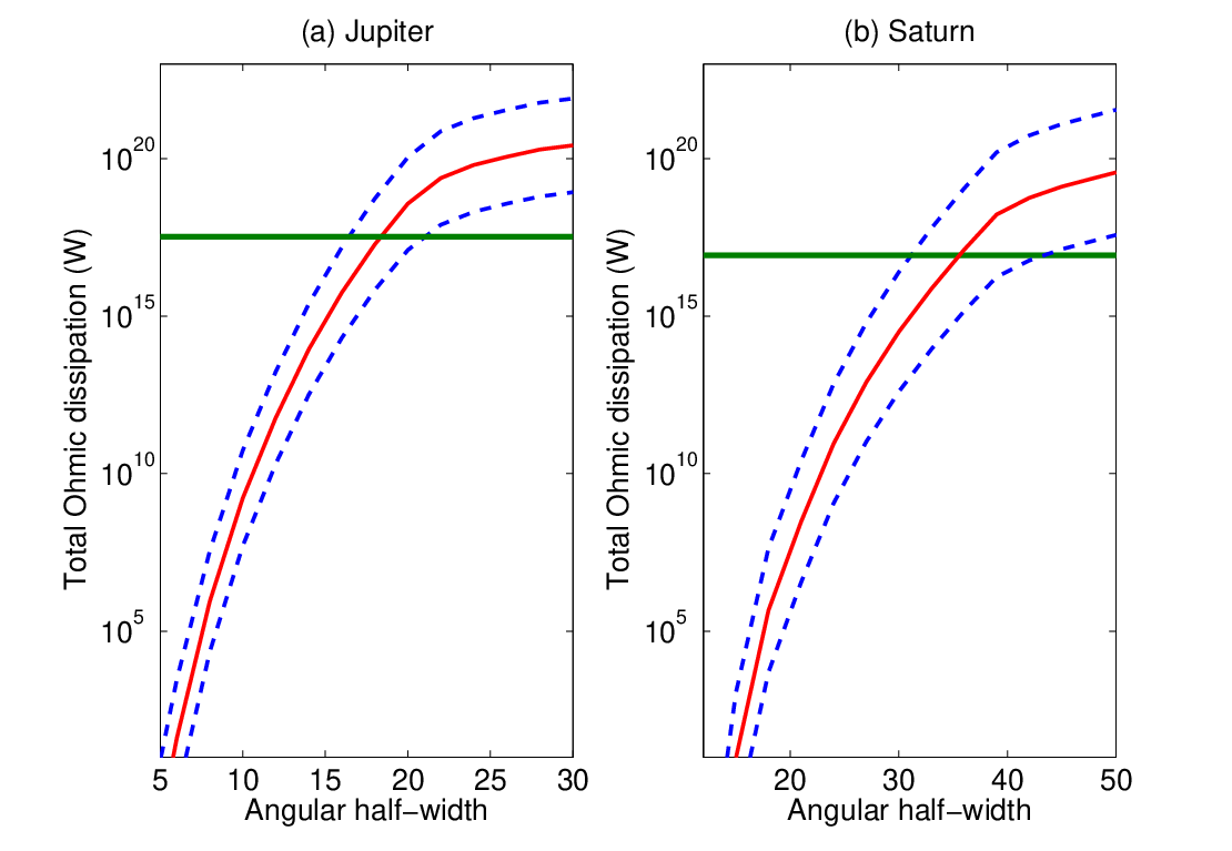
d Maximum width of an equatorial jet
A sufficiently narrow equatorial jet could maintain constant velocity on cylinders throughout the planet. As an example, we consider the specific velocity profile
| (44) |
and,
| (45) |
so the jet has equatorial velocity and angular half-width . For Jupiter and Saturn, is approximately and , respectively. Figure (10) displays the calculated Ohmic dissipation rate as a function of the jet half-width. The maximum half-width is about for Jupiter, and for Saturn. The maximum half widths are related to the fractional radii of maximum penetration, , calculated in section 3 by
| (46) |
6 Discussion.
The condition that the total Ohmic dissipation not exceed the planet’s net luminosity sets an upper bound on the depth to which the zonal flows observed in the atmospheres of Jupiter and Saturn could penetrate. At these depths, the magnetic Reynolds number, based on the observed zonal winds and the scale height of the magnetic diffusivity, is of order unity.
We consider it unlikely that the observed flows extend to the depth of maximum penetration because that would require the Taylor-Proudman constraint to be violated in the convective envelope. We have been unable to identify any plausible mechanism that could do this. Lack of a rigorous model for convection is a weakness. We base our analysis of the robustness of the Taylor-Proudman constraint on the mixing length model designed by Ingersoll & Pollard 1982 to apply under conditions of strong differential rotation. However, we have confirmed that the conclusions we draw from it also follow from other convection models that consider only solid body rotation, or even those that neglect the effects of rotation entirely.
The boundaries of the cylindrical extensions of the equatorial jets essentially coincide with the maximum penetration depths. Thus these jets could maintain constant velocities along cylinders through the planets. Winds measured at by the Galileo probe as it descended into Jupiter are consistent with this possibility.
Acknowledgments
We are grateful for support from the NASA Planetary Geology and Geophysics program.
7 Appendix


We calculate the current distribution arising from a vacuum axial dipole field and a simple zonal flow. The angular velocity, , is taken to be of the form
| (47) |
Here is the truncation factor and is the truncation radius. for and for .88 8 We plot as a function of scaled radius in figure (11).
The current density arising from interaction of this flow with a vacuum dipole magnetic field satisfies:
| (48) |
where is the dipole moment.
Because , can be derived from a vector potential such that
| (49) |
where
| (50) |
By direct computation
| (51) |
So
| (52) |
At the planet’s surface, the current density along the radial direction goes to zero: ; Near its center, : . We solve equation (52) to obtain .
Since,
| (53) |
the current density follows the contour lines of and its magnitude satisfies . Figure (12) displays the streamlines of current flow.
References
- Ashcroft (1968) Ashcroft, N. W. 1968. Metallic hydrogen - a high temperature superconductor. Phys. Rev. Lett. 21, 1748–1749.
- Atkinson et al. (1997) Atkinson, D. H., A. P. Ingersoll and A. Seiff 1997. Deep zonal winds on Jupiter: update of Doppler tracking the Galileo probe from the orbiter. Nature 338, 649–650.
- Atkinson et al. (1998) Atkinson, D. H., J. B. Pollack and A. Seiff 1998. The Galileo probe Doppler wind experiment: measurement of the deep zonal wind on Jupiter. J. Geophys. Res 103, 22911–22928.
- Aurnou & Heimpel (2004) Aurnou, J. M., and M. H. Heimpel 2004. Zonal jets in rotating convection with mixed mechanical boundary conditions. Icarus 169, 492–498.
- Busse (1976) Busse, F. H. 1976. Simple model of convection in the Jovian atmosphere. Icarus 29, 255–260.
- Busse (1983) Busse, F. H. 1983. A model of mean zonal flows in the major planets. Geophys. Astrophys. Fluid. Dyn. 23(2), 153–174.
- Busse (1994) Busse, F. H. 1994. Convection driven zonal flows and vortices in the major planets. Chaos 4, 123–134.
- Connerney (1993) Connerney, J. E. P. 1993. Magnetic field of the outer planets. J. Geophys. Res. 98, 18659–18679.
- Dessler (1983) Dessler, A. J. 1983. Coordinate systems. Physics of the Jovian magnetosphere Cambridge University Press, New York, pp. 498–504
- Glatzmaier (2005) Glatzmaier, G. A. 2005 A saturnian dynamo simulation. American Geophysical Union Fall Meeting 2005, San Francisco, CA
- Guillot (1999) Guillot, T. 1999 A comparison of the interiors of Jupiter and Saturn. Plan. Space Sci., 47, 1183–1200
- Guillot et al. (2004) Guillot, T., D. J. Stevenson, W. B. Hubbard and D. Saumon 2004 The interior of Jupiter. Jupiter: The Planet, Satellites and Magnetosphere Cambridge University Press, New York, pp 35–57
- Guillot (2005) Guillot, T. 2005. The interior of giant planets: Models and outstanding questions. Annu. Rev.Earth Planet Sci., 33, 493–530
- Heimpel et al. (2005) Heimpel, M., J. Aurnou and J. Wicht 2005. Simulation of equatorial and high latitude jets on Jupiter in a deep convection model. Nature 438, 193–196
- Holmes et al. (1995) Holmes, N. C., M. Ross and W. J. Nellis 1995. Temperature measurements and dissociation of shock-compressed liquid deuterium and hydrogen. Phys. Rev. B 59, 15835–15845
- Hubbard (1968) Hubbard, W. B. 1968. Thermal structure of Jupiter. Astrophys. J. 152(3P1), 745–754.
- Hubbard et al. (1997) Hubbard, W. B., T. Guillot, and J. I. Lunine 1997. Liquid metallic hydrogen and the structure of brown dwarfs and giant planets. Phys. Plasmas. 4(5), 2011–2015
- Ingersoll & Cuzzi (1969) Ingersoll, A. P. and J. N. Cuzzi 1969. Dynamics of Jupiter’s cloud bands. J. Atmos. Sci. 26, 981–985.
- Ingersoll & Pollard (1982) Ingersoll, A. P. and D. Pollard 1982. Motion in the interiors and atmosphere of Jupiter and Saturn -scale analysis, anelastic equations, barotropic-stability criterion. Icarus 52, 62–80.
- Ingersoll et al. (1984) Ingersoll, A. P., R. F. Beebe, B. J. Conrath and G. E. Hunt 1984. Structure and dynamics of Saturn’s atmosphere. Saturn University of Arizona Press, Tucson, pp 195–238
- Ingersoll (1990) Ingersoll, A. P. 1990. Atmospheric dynamics of the outer planets. Science 248, 308–315.
- Liu (2006) Liu, J. J. 2006. Interaction of magnetic field and zonal wind in the out shells of giant planets. Caltech Thesis 2006, 47–52.
- Nellis et al. (1992) Nellis, W. J., A. C. Mitchell, P. C. McCandless, D. J. Erskine and S. T. Weir 1992. Electronic energy gap of molecular hydrogen from electrical conductivity measurements at high shock pressures. Phys. Rev. Lett. 68, 2937–2940
- Nellis et al. (1995) Nellis, W. J., M. Ross and N. C. Holmes 1995. Temperature measurements of shock-compressed liquid hydrogen: implication for the interior of Jupiter Science 269, 1249–1252
- Nellis et al. (1996) Nellis, W. J., S. T. Weir and A. C. Mitchell 1996. Metallization and electrical conductivity of fluid hydrogen in Jupiter. Science 273, 936–938
- Nellis et al. (1999) Nellis, W. J., S. T. Weir and A. C. Mitchell 1999. Minimum metallic conductivity of fluid hydrogen at 140 GPa (1.4 Mbar). Phys. Rev. B. 59, 3434–3449
- Porco et al. (2003) Porco, C. C., et al. 2003 Cassini imaging of Jupiter’s atmosphere, satellites and rings. Science 299, 1541–1547
- Porco et al. (2005) Porco, C. C., et al. 2005 Cassini imaging science: initial results on Saturn’s atmosphere. Science 307, 1243–1247
- Russell et al. (2001a) Russel, C. T., Z. J. Yu, K. K. Khurana and M. G. Kivelson 2001. Magnetic field changes in the inner magnetosphere of Jupiter. Adv. Space Res. 28(6), 897–902.
- Russell et al. (2001b) Russel, C. T., Z. J. Yu, K. K. Khurana, S. P. Joy and M. G. Kivelson 2001. Secular variation of the Jovian magnetic field from singular value decomposition analysis American Astronomical Society, DPS meeting 33, 1097.
- Smith & Hunt (1976) Smith, B. A. and G. E. Hunt 1976. Motions and morphology of clouds in the atmosphere of Jupiter. Jupiter University of Arizona Press, Tucson, pp 564-585
- Stevenson & Ashcroft (1974) Stevenson D. J. and N. W. Ashcroft 1974. Conductions in fully ionized liquid-metals Phys. Rev. A 9(2), 782–789.
- Taylor (1923) Taylor, G. I. 1923. Experiments on the motion of solid bodies in rotating fluids. Proc. R. Soc. A 104, 213–218.
- Vasavada & Showman (2005) Vasavada A. R. and A. P. Showman 2005. Jovian atmospheric dynamics: An update after Galileo and Cassini. Rep. Prog. Phys. 68, 1935-1996.
- Weir et al. (1996) Weir, S. T., A. C. Mitchell and W. J. Nellis 1996. Metallization of fluid molecular hydrogen at 140 Gpa. Phys. Rev. Lett. 76, 1860–1863.