Nonequilibrium work distribution of a quantum harmonic oscillator

Fluctuations play a fundamental role in small nonequilibrium systems. While thermodynamic quantities like the free energy difference can easily be calculated for slow, quasistatic processes from the knowledge of the initial and final equilibrium partition functions, $\Delta F=F_{1}-F_{0}=-kT\ln Z_{1}/Z_{0}$, a general method for evaluating $\Delta F$ in the case of fast, nonequilibrium transformations was lacking until recently. A decade ago, Jarzynski introduced a remarkable equality that relates the free energy difference to the averaged exponentiated work done during the process jar97,

with $\langle e^{-\beta W}\rangle=\int dWe^{-\beta W}\,P(W)$ and $\beta=1/kT$ the inverse temperature. Equation (1) allows to compute the difference $\Delta F$ for arbitrary transformations, quasistatic or not, once the corresponding distribution of work $P(W)$ is known. The free energy difference is thus entirely determined by the fluctuations of the total work $W$, a property which emphasizes the importance of the work probability density. The usefulness of Eq. (1) for evaluating $\Delta F$ in single biomolecules has been demonstrated in DNA unfolding experiments lip02; bus05.

Extensions of the classical Jarzynski equality (1) to quantum–mechanical systems have been discussed in Refs. tas00; muk03; mae04; che04; mon05; tal07a; tal07b. In that respect, it is worth mentioning that the concept of work in quantum thermodynamics has been clarified in Ref. tal07a. Thus for a quantum Hamiltonian system, work cannot be considered as the expectation value of some work operator, in contrast to some other thermodynamic quantities like energy. Rather the exponential average of the work, as well as its characteristic function, are given by time-ordered quantum correlation functions.

Our aim in this paper is to determine the work distribution for a simple quantum system, namely a time–dependent harmonic oscillator. We obtain the exact analytical expression of the characteristic function of the work and provide approximations for the work distribution for adiabatic and nonadiabatic processes, in the limit of low and high temperature. Moreover, we check the validity of the Jarzynski equality for arbitrary processes.

We consider a quantum–mechanical harmonic oscillator with a time-dependent angular frequency $\omega(t)$. The corresponding Hamiltonian is of the usual form

We shall be interested in calculating the work distribution of the oscillator when the angular frequency is changed from an initial value $\omega_{0}$ at $t=0$ to a final value $\omega_{1}$ at $t=\tau$. We denote by $\phi_{n}^{t}$ the eigenfunctions and by $E_{n}^{t}=\hbar\omega(t)(n+\frac{1}{2})$ the eigenvalues of the Hamiltonian (2) at any given time $t$. We make the additional assumption that the oscillator is initially thermalized with inverse temperature $\beta$ but is otherwise isolated.

The probability density of the total work done on the harmonic oscillator during time $\tau$ is given by tal07a

where $P_{n}^{0}=\exp(-\beta E_{n}^{0})/Z_{0}$ is the initial (thermal) occupation probability and $P_{m,n}^{\tau}$ are the transition probabilities between initial and final states $n$ and $m$,

The evaluation of the transition probabilities (4) requires the computation of the propagator $U(x,x_{0};\tau)$ of the time–dependent harmonic oscillator. To this end, we follow the approach developed by Husimi 2.

The dynamics generated by the quadratic Hamiltonian (2) is Gaussian for any $\omega(t)$. By introducing the Gaussian wave function ansatz,

the Schrödinger equation for the quantum oscillator can be reduced to a system of three coupled differential equations for the parameters $a,b$ and $c$,

The nonlinear equation (6) is of the Riccati type. Writing $a=\frac{m\dot{X}}{X}$, it can be mapped to the equation of motion of a classical time–dependent linear oscillator,

The solutions of Eqs. (6)–(8), and hence the wave function (5) of the quantum oscillator, can be recurrently constructed from the solution of Eq. (9). An explicit solution of Eq. (9) for the linear parametrization jar97a,

is given in Appendix A. We stress that the following results are valid for arbitrary $\omega(t)$.

The general form of the propagator can be determined from the wave function (5) by noting that $\phi(x,\tau)=\int dx\,U(x,x_{0};\tau)\,\phi(x_{0},0)$. It is explicitly given by

where $X(t)$ and $Y(t)$ are solutions of Eq. (9) satisfying

A compact expression for the generating function of the transition probabilities $P_{m,n}^{\tau}$ can then be obtained by using the generating functions of the eigenfunctions $\phi_{n}^{t}(x)$ of the quantum harmonic oscillator,

By exploiting the Gaussian character of Eqs. (11) and (II), the generating function of Eq. (4) becomes

where we have introduced the quantity

The parameter $Q^{*}$ will play an important role in the following discussion. We will indeed see that it can be regarded as a measure of the degree of adiabaticity of the process. An interesting feature of the generating function $P(u,v)$ is further that its $(u,v)$–dependence remains the same for all possible transformations $\omega(t)$. Details about the specific parametrization of the angular frequency only enter through different numerical values of $Q^{*}$.

With the help of Eq. (II), the characteristic function of the work, defined as the Fourier transform of the probability distribution (3),

can eventually be written in closed form in terms of the energies, $\varepsilon_{0}=\hbar\omega_{0}$, $\varepsilon_{1}=\hbar\omega_{1}$ ($\Delta\varepsilon=\varepsilon_{1}-\varepsilon_{0}$) and the inverse temperature $\beta$. We have

The above expression for $G(\mu)$ is exact and fully characterizes the work distribution of the time–dependent quantum harmonic oscillator (2), for arbitrary parametrization of the angular frequency $\omega(t)$. As mentioned previously, different realizations of $\omega(t)$ will merely lead to different values of the parameter $Q^{*}$. One should also note that the mass $m$ of the oscillator does not explicitly appear in (17).

The direct analytic evaluation of the nonequilibrium work distribution $P(W)$ by Fourier inverting Eq. (17) does not seem to be feasible in the general case. In this section, we derive approximate expressions of the work probability density for adiabatic and nonadiabatic processes, in the zero and high–temperature limit.

The parameter $Q^{*}$ defined in Eq. (15) can be ascribed a simple physical meaning 2. Let us consider a transition from initial state $n$ to final state $m$. Then the average quantum number in the final state is

which follows from the expression of the generating function (II) of $P_{m,n}^{\tau}$. Similarly, the mean–square quantum number after time $\tau$ is given by

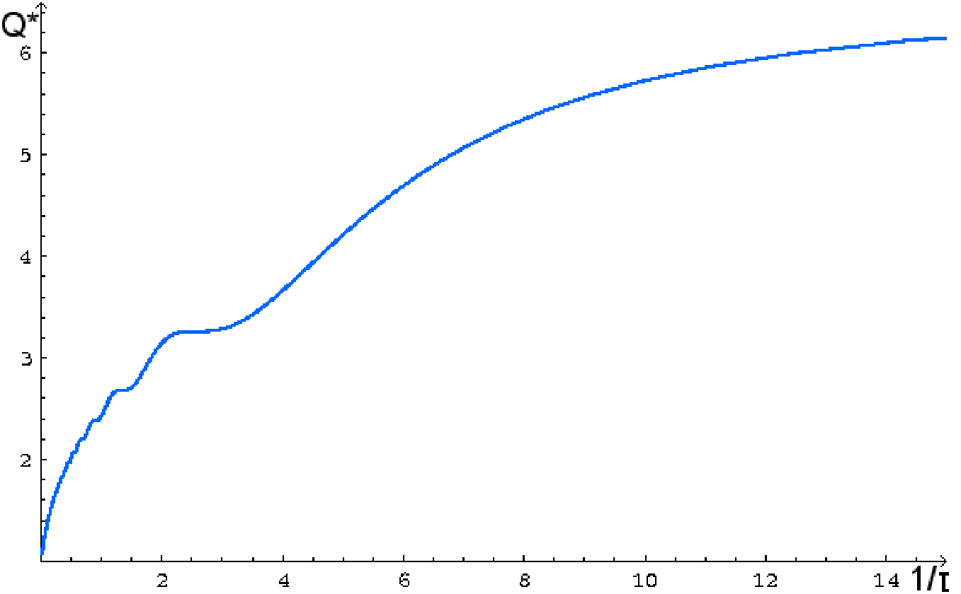
Equation (31) shows that the parameter $Q^{*}$ directly controls the magnitude of the variance $\sigma^{2}_{m,n}$. In the adiabatic limit, $Q^{*}=1$, we readily get $\langle m\rangle_{n}=n$ and $\sigma^{2}_{m,n}=0$. We therefore recover that for quasistatic processes, the system remains in its initial state, $m=n$. On the other hand, for fast nonadiabatic processes, the mean $\langle m\rangle_{n}$ and the dispersion $\sigma^{2}_{m,n}$ increase with increasing values of $Q^{*}$, indicating that the quantum oscillator ends in a final state $m$ which is farther and farther away from the initial state $n$. The behavior of $Q^{*}$ as a function of the inverse switching time $1/\tau$ is shown in Fig. (3) for the linear parametrization (10) with fixed values of the initial and final angular frequencies. We observe, as expected, that infinitely slow switching, $1/\tau\rightarrow 0$, corresponds to the adiabatic limit $Q^{*}\rightarrow 1$, while, for finite–time transformations, the parameter $Q^{*}$ monotonically increases with the inverse switching time.

The adiabatic and nonadiabatic work distributions Eqs. (22), (24) and Eqs. (27), (29) are plotted in Figs. (1) and (2). They illustrate the effect of temperature and nonadiabaticity on the probability density $P(W)$ of the harmonic oscillator. The mean and the variance of the work probability distribution, as well as the mean dissipated work can be found in Appendix B. Let us begin with Fig. (2). For an adiabatic transformation at zero temperature, the oscillator remains in the ground state for all times. As a consequence, the total work and the free energy difference are equal to the energy difference between the initial and final ground states, $W=\Delta F=\Delta\varepsilon/2$. In this case, $P(W)$ is simply a delta function. As we now increase the temperature, the initial thermal distribution broadens. This then results in a widening of the work distribution to a one–sided exponential in the high–temperature limit as seen in Fig. (1). On the other hand, when the nonadiabaticity parameter $Q^{*}$ is augmented, we observe still in Fig. (1) that the work distribution acquires a negative tail. This is a remarkable fact since for a process with negative total work, the quantum harmonic oscillator is cooled when its angular frequency is varied and not heated. This situation can obviously not occur when the oscillator is already in its ground state, explaining the absence of a negative tail in the nonadiabatic work distribution in Fig. (2). Here the broadening of the distribution $P(W)$ is related to the work which is dissipated when the oscillator is brought to an excited state.

We have analytically calculated the characteristic function of the total work of a quantum harmonic oscillator with a time–dependent angular frequency. We have obtained approximate formulas for the work distribution for the case of adiabatic and nonadiabatic transformations, in the limit of low and high temperature. We have further checked the validity of the quantum Jarzynski equality for arbitrary parametrizations of the angular frequency and discussed the effect of temperature and nonadiabaticity of the work probability density.

The equation of motion for the time–dependent harmonic oscillator (9) can in general not be solved exactly. In this appendix, we provide the analytical solutions of Eq. (9) for the linear parametrization (10) of the angular frequency, obeying the boundary conditions (II). They can expressed with the help of the Airy-A and Airy-B functions 17,

and

where $Ai^{\prime}(x)$ and $Bi^{\prime}(x)$ denote the first derivatives with respect to $x$.

In this appendix, we evaluate the mean and the variance of the work probability distribution, as well as the mean dissipated work for the frequency–dependent quantum harmonic oscillator. We use the formulas,

We consider the general expression (17) for the characteristic function of the work $G(\mu)$ as well as the various approximations (21), (23), (25) and (28) obtained in the high and low temperature limit and for adiabatic and nonadiabatic transformations. The free energy difference $\Delta F$ is given by Eq. (12). In the quantum limit $\hbar\beta\gg 1$, the free energy difference simplifies to

whereas in the classical limit $\hbar\beta\ll 1$, one has

Note that for an adiabatic transformation $Q^{*}=1$ and $\Delta\omega/\omega_{0}\ll 1$, so that in this case $\Delta F\simeq\Delta\omega/\beta$. $\langle W\rangle$ $\langle W^{2}\rangle-\langle W\rangle^{2}$ $\langle W_{dis}\rangle$ General $Q^{*}\neq 1$ $\frac{1}{2}(Q^{*}\varepsilon_{1}-\varepsilon_{0})\coth{[\frac{\beta}{2}\varepsilon_{0}]}$ $\frac{({Q^{*}}^{2}\varepsilon_{1}-\varepsilon_{0})^{2}+({Q^{*}}^{2}-1)\varepsilon_{1}^{2}\cosh{[\beta\varepsilon_{0}]}}{4\sinh^{2}{[\frac{\beta}{2}\varepsilon_{0}]}}$ $\frac{1}{\beta}\ln{\Bigg[\frac{(e^{\beta\varepsilon_{0}}+1)(\varepsilon_{0}-Q^{*}\varepsilon_{1})+2(e^{\beta\varepsilon_{0}}-1)\frac{\sinh{[\frac{\beta}{2}\varepsilon_{0}]}}{\sinh{[\frac{\beta}{2}\varepsilon_{1}]}}}{2(e^{\beta\varepsilon_{0}}-1)}\Bigg]}$ Eq. (17) General $Q^{*}=1$ $\frac{1}{2}(\varepsilon_{1}-\varepsilon_{0})\coth{[\frac{\beta}{2}\varepsilon_{0}]}$ $\frac{1}{4}(\varepsilon_{1}-\varepsilon_{0})^{2}\frac{1}{\sinh^{2}{[\frac{\beta}{2}\varepsilon_{0}]}}$ $0$ Eq. (17) $\hbar\beta\ll 1$ $Q^{*}\neq 1$ $\frac{1}{\beta\omega_{0}}\big(Q^{*}\omega_{1}-\omega_{0}\big)$ $\frac{1}{\beta^{2}\omega_{0}^{2}}\big(\omega_{0}^{2}-2Q^{*}\omega_{0}\omega_{1}+(2{Q^{*}}^{2}-1)\omega_{1}^{2}\big)$ $\frac{1}{\beta}\big(\frac{Q^{*}\omega_{1}-\omega_{0}}{\omega_{0}}-\ln{[\frac{\omega_{1}}{\omega_{0}}]}\big)$ Eq. (25) $\hbar\beta\ll 1$ $Q^{*}=1$ $\frac{1}{\beta\omega_{0}}\big(\omega_{1}-\omega_{0}\big)$ $\frac{1}{\beta^{2}\omega_{0}^{2}}\big(\omega_{1}-\omega_{0}\big)^{2}$ $0$ Eq. (21) $\hbar\beta\gg 1$ $Q^{*}\neq 1$ $\frac{1}{2}(Q^{*}\varepsilon_{1}-\varepsilon_{0})$ $\frac{1}{2}({Q^{*}}^{2}-1)\varepsilon_{1}^{2}$ $\frac{1}{2}(Q^{*}-1)\varepsilon_{1}$ Eq. (28) $\hbar\beta\gg 1$ $Q^{*}=1$ $\frac{1}{2}(\varepsilon_{1}-\varepsilon_{0})$ $0$ $0$ Eq. (23)

References

- (1) C. Jarzynski, Phys. Rev. Lett. 78, 2690 (1997).
- (2) J. Liphard et al., Science 296, 1842 (2002).
- (3) C. Bustamante, J. Liphardt, and F. Ritort, Phys. Today 58(7), 43 (2005).
- (4) H. Tasaki, e-print arXiv:cond-mat/0009244v2.
- (5) S. Mukamel, Phys. Rev. Lett. 90, 170604 (2003).
- (6) W. De Roeck and C. Maes, Phys. Rev. E 69, 026115 (2004).
- (7) V. Chernyak and S. Mukamel, Phys. Rev. Let. 93, 048302 (2004).
- (8) T. Monnai, Phys. Rev. E 72, 027102 (2005).
- (9) P. Talkner, E. Lutz and P. Hänggi, Phys. Rev. E 75, 050102 (2007)(R).
- (10) P. Talkner and P. Hänggi, J. Phys. A 40, F569 (2007).
- (11) K. Husimi, Prog. Theo. Phys. 9, 381 (1953).
- (12) C. Jarzynski, Phys. Rev. E 56, 5018 (1997).
- (13) H. Callen,Thermodynamics and an Introduction to Thermostatistics (Wiley, New York, 1985).
- (14) A.P. Prudnikov, Y.A. Brychow, and O.I. Marichev, Integrals and Series (Gordon and Breach, Amsterdam, 1990), Vol.1.
- (15) A.P. Prudnikov, Y.A. Brychow, and O.I. Marichev, Integrals and Series (Gordon and Breach, Amsterdam,1990), Vol.2.