The Stochastic Green Function (SGF) algorithm

V.G. Rousseau Affiliation: Instituut-Lorentz, LION, Universiteit Leiden, Postbus 9504, 2300 RA Leiden, The Netherlands

Abstract

We present the Stochastic Green Function (SGF) algorithm designed for bosons on lattices. This new quantum Monte Carlo algorithm is independent of the dimension of the system, works in continuous imaginary time, and is exact (no error beyond statistical errors). Hamiltonians with several species of bosons (and one-dimensional Bose-Fermi Hamiltonians) can be easily simulated. Some important features of the algorithm are that it works in the canonical ensemble and gives access to n-body Green functions.

pacs

05.30.Jp,02.70.Uu

I Introduction

In the last twenty years, numerical methods have gained importance with the increasing power of computers. They have been solicited in situations where analytical results are missing, due to the complexity of the studied problems, and where approximate methods fail to give a correct description. But even with computers, exact calculations are often limited to special cases. This is especially true for quantum many-body problems where the size of the Hilbert space grows exponentially with the size of the system, restricting exact diagonalizations to very small systems. Quantum Monte Carlo (QMC) methods have been developed in order to simulate bigger systems, and allow a correct description of quantum fluctuations, which are usually missed by mean-field theories Rigol04. QMC methods have given rise to various kinds of algorithms Rigol03; Blankenbecler; White; Batrouni1990; Batrouni1992; Sandvik; Prokofev; Rousseau2005; VanHoucke06; Rombouts06.

We propose here a new algorithm designed for bosons on lattices, the Stochastic Green Function (SGF) algorithm. The algorithm is independent of the dimension of the system, and works in continuous imaginary time. The algorithm is exact, in the sense that it has no error beyond statistical errors. Hamiltonians with several species of bosons Rousseau2007; Timmermans; Sengupta2005 (and one-dimensional Bose-Fermi mixtures Pollet06; Sengupta07; Hebert06) are easily treated. An important property is that the SGF algorithm works in the canonical ensemble. This is especially important when working with several species of particles, because it is numerically difficult to control several numbers of particles in the grand-canonical ensemble. Indeed, working with several species in the grand-canonical ensemble requires one chemical potential per species. Those chemical potentials have to be tuned to find the desired number of particles. But the difficulty comes from the fact that the number of particles of a given species depends on all chemical potentials. Working in the canonical ensemble makes things much simpler, by just choosing the number of particles for each species. Another property of the algorithm is that it provides access to n-body Green functions, allowing the calculation of momentum distribution functions which are important for the connection between theory and experiments.

II Motivations

We consider a Hamiltonian of the form

\hat{\mathcal{H}}=\hat{\mathcal{V}}-\hat{\mathcal{T}},

(1)

where $\hat{\mathcal{V}}$ and $\hat{\mathcal{T}}$ are respectively diagonal and non-diagonal (positive definite) operators. We would like to have at our disposal an algorithm that is simple and able to simulate any Hamiltonian of the form (1), in the canonical ensemble (for the reason above). As an example, we will consider a Hamiltonian describing two species of particles, atoms and diatomic molecules. The particles from one species interact together, and interact with particles of the other species. We also take into account the possibility for atoms to be converted into molecules, and vice-versa. The situation can be described by the following $\hat{\mathcal{V}}$ and $\hat{\mathcal{T}}$ operators:

$\displaystyle\hat{\mathcal{V}}$	$\displaystyle=$	$\displaystyle U_{aa}\sum_{i}\hat{n}_{i}^{a}\big(\hat{n}_{i}^{a}-1\big)+U_{mm}\sum_{i}\hat{n}_{i}^{m}\big(\hat{n}_{i}^{m}-1\big)$	(2)
	$\displaystyle+$	$\displaystyle U_{am}\sum_{i}\hat{n}_{i}^{a}\hat{n}_{i}^{m}+\!D\sum_{i}\hat{n}_{i}^{m}$	(2)
$\displaystyle\hat{\mathcal{T}}$	$\displaystyle=$	$\displaystyle t_{a}\sum_{\big\langle i,j\big\rangle}\big(a_{i}^{\dagger}a_{j}^{\phantom{\dagger}}+h.c.\big)+t_{m}\sum_{\big\langle i,j\big\rangle}\big(m_{i}^{\dagger}m_{j}^{\phantom{\dagger}}+h.c.\big)$	(3)
	$\displaystyle+$	$\displaystyle g\sum_{i}\big(m_{i}^{\dagger}a_{i}^{\phantom{\dagger}}a_{i}^{\phantom{\dagger}}+a_{i}^{\dagger}a_{i}^{\dagger}m_{i}^{\phantom{\dagger}}\big)$	(3)

$\hat{\mathcal{V}}$ and $\hat{\mathcal{T}}$ correspond respectively to the potential and kinetic+conversion energies. The $a_{i}^{\dagger}$ and $a_{i}^{\phantom{\dagger}}$ operators ( $m_{i}^{\dagger}$ and $m_{i}^{\phantom{\dagger}}$ ) are the creation and annihilation operators of atoms (molecules) on site $i$ , and $\hat{n}_{i}^{a}=a_{i}^{\dagger}a_{i}^{\phantom{\dagger}}$ ( $\hat{n}_{i}^{m}=m_{i}^{\dagger}m_{i}^{\phantom{\dagger}})$ counts the number of atoms (molecules) on site $i$ . The sum $\big\langle i,j\big\rangle$ is over pairs of first nearest neighbors. We can see that the $\hat{\mathcal{T}}$ operator allows atoms and molecules to jump onto neighboring sites, and that two atoms can be transformed into one molecule (and vice-versa). The total number of atoms $N_{a}=\sum_{i}\hat{n}_{i}^{a}$ and the total number of molecules $N_{m}=\sum_{i}\hat{n}_{i}^{m}$ are not conserved, however the number $N=N_{a}+2N_{m}$ is conserved. This is our canonical constraint. We will not discuss at all the physics of this Hamiltonian, referring the interested reader to the literature Rousseau2007; Timmermans; Sengupta2005.

Among existing QMC algorithms, the Canonical Worm (CW) algorithm VanHoucke06; Rombouts06 is a good choice if one wants to work in the canonical ensemble and to have access to Green functions. However this algorithm makes use of a ”worm operator” $\hat{\mathcal{W}}$ , and some complexity of the algorithm arises when $\hat{\mathcal{T}}$ does not commute with $\hat{\mathcal{W}}$ (see section III.B). It is always possible to make the trivial choice $\hat{\mathcal{W}}=1+\hat{\mathcal{T}}$ for the worm operator which leads to a zero commutator, $\big[\hat{\mathcal{W}},\hat{\mathcal{T}}\big]=0$ . But such a choice is not appropriate at all when the $\hat{\mathcal{T}}$ operator connects only neighboring sites (which is usually the case). Indeed this would lead to a worm operator that is unable to generate spatial discontinuities of the worldlines for which the broken parts are separated by more than one lattice site. Therefore it would be impossible to measure Green functions which require long range discontinuities of the worldlines. Moreover, this choice for the worm operator generates only local updates, which are known to be much less efficient than global updates. Finally, those local updates cannot sample the winding, which is a quantity of interest when working with periodic boundary conditions. As a result, a more complicated choice has to be made for $\hat{\mathcal{W}}$ . For our chosen $\hat{\mathcal{T}}$ operator, it is not trivial to find a suitable $\hat{\mathcal{W}}$ operator that commutes with $\hat{\mathcal{T}}$ and satisfies the requirements just mentioned. While a suitable $\hat{\mathcal{W}}$ operator might exist, we have not managed to find one that can be easily handled. Reference [10] proposes an extension of the applicability of the worm operator, but this goes beyond our purposes of simplicity and generality. The SGF algorithm we propose is an alternative way to simulate any Hamiltonian of the form (1) in a very simple and general way. Basically, once one has a SGF computer code that simulates a given Hamiltonian, the only thing to do to extend the code to another Hamiltonian is to change the definition of the Hamiltonian in the code.

III The algorithm

III.1 The partition function and the ”Green operator”

The SGF algorithm is derived from the CW algorithm. We start by considering the partition function $\mathcal{Z}(\beta)=\textrm{Tr }e^{-\beta\hat{\mathcal{H}}}$ , and we perform the expansion

	$\displaystyle\!\!\!\!\!\!\!\!\mathcal{Z}(\beta)\!$	$\displaystyle=$	$\displaystyle\textrm{Tr }e^{-\beta\hat{\mathcal{V}}}T_{\tau}e^{\int_{0}^{\beta}\hat{\mathcal{T}}(\tau)d\tau}$		(4)
		$\displaystyle=$	$\displaystyle\textrm{Tr}\sum_{n=0}^{+\infty}\int_{0<\tau_{1}<\cdots<\tau_{n}<\beta}\hskip-56.9055pte^{-\beta\hat{\mathcal{V}}}\hat{\mathcal{T}}(\tau_{n})\cdots\hat{\mathcal{T}}(\tau_{2})\hat{\mathcal{T}}(\tau_{1})d\tau_{1}\cdots d\tau_{n},$		(4)

where $T_{\tau}$ is the ”time ordering” operator and $\hat{\mathcal{T}}(\tau)$ is defined by

\hat{\mathcal{T}}(\tau)=e^{\tau\hat{\mathcal{V}}}\hat{\mathcal{T}}e^{-\tau\hat{\mathcal{V}}}.

(5)

By introducing complete sets of states $I=\sum_{\psi}\big|\psi\big\rangle\big\langle\psi\big|$ between each non-diagonal operator $\hat{\mathcal{T}}$ , we get

$\displaystyle\mathcal{Z}(\beta)\!\!\!$	$\displaystyle=$	$\displaystyle\!\!\!\sum\int_{0<\tau_{1}<\cdots<\tau_{n}<\beta}\hskip-56.9055pt\big\langle\psi_{0}\big\|e^{-\beta\mathcal{V}}\hat{\mathcal{T}}(\tau_{n})\big\|\psi_{n-1}\big\rangle\big\langle\psi_{n-1}\big\|\hat{\mathcal{T}}(\tau_{n-1})\big\|\psi_{n-2}\big\rangle$	(6)
	$\displaystyle\times$	$\displaystyle\cdots\big\langle\psi_{k}\big\|\hat{\mathcal{T}}(\tau_{k})\big\|\psi_{k-1}\big\rangle\cdots$
	$\displaystyle\times$	$\displaystyle\big\langle\psi_{2}\big\|\hat{\mathcal{T}}(\tau_{2})\big\|\psi_{1}\big\rangle\big\langle\psi_{1}\big\|\hat{\mathcal{T}}(\tau_{1})\big\|\psi_{0}\big\rangle d\tau_{1}\cdots d\tau_{n}.$

Using the notation $V_{k}$ for the eigenvalue of $\hat{\mathcal{V}}$ in the eigenstate $\big|\psi_{k}\big\rangle$ , $V_{k}=\big\langle\psi_{k}\big|\hat{\mathcal{V}}\big|\psi_{k}\big\rangle$ , each matrix element in (6) takes the form

\big\langle\psi_{k}\big|\hat{\mathcal{T}}(\tau)\big|\psi_{l}\big\rangle=e^{\tau V_{k}}\big\langle\psi_{k}\big|\hat{\mathcal{T}}\big|\psi_{l}\big\rangle e^{-\tau V_{l}}.

(7)

It is useful here to give an interpretation of expression (6). We assume for the simplicity of this interpretation that we have only one species of particles on a one-dimensional lattice, and that the $\hat{\mathcal{T}}$ operator is the usual one-body operator that makes the particles jump onto neighboring sites. The partition function is a sum over all possible configurations of time indices $\tau_{1},\cdots,\tau_{n}$ and states $\big\{\big|\psi_{k}\big\rangle\big\}$ . Figure 1 (left image) shows a representation of a possible configuration. We start at imaginary time $\tau=0$ with a state $\big|\psi_{0}\big\rangle$ that contains 3 particles. Then the state evolves with the operator $e^{-\tau_{1}V_{0}}$ until time $\tau_{1}$ . During this evolution, the state does not change because the $\hat{\mathcal{V}}$ operator is diagonal. At time $\tau_{1}$ a $\hat{\mathcal{T}}$ operator acts onto the state, leading to a sum of several new states. In this sum of states, only the state $\big|\psi_{1}\big\rangle$ survives when making the scalar product with the bra $\big\langle\psi_{1}\big|$ . This new state differs from $\big|\psi_{0}\big\rangle$ by a jump of only one particle, since we have assumed in our example that $\hat{\mathcal{T}}$ is a one-body operator. Thus at time $\tau_{1}$ one particle jumps onto a neighboring site. The new state $\big|\psi_{1}\big\rangle$ then evolves without changing with the operator $e^{-(\tau_{2}-\tau_{1})V_{1}}$ until time $\tau_{2}$ . At time $\tau_{2}$ one particle jumps onto a neighboring site leading to the new state $\big|\psi_{2}\big\rangle$ … and so on, until time $\tau_{n}$ where a last jump of one particle leads to the initial state $\big|\psi_{0}\big\rangle$ , which evolves without changing with the operator $e^{-(\beta-\tau_{n})V_{n}}$ until time $\beta$ . As a result, one configuration of time indices $\tau_{1},\cdots,\tau_{n}$ and states $\big\{\big|\psi_{k}\big\rangle\big\}$ corresponds to a set of lines (the worldlines) that the particles follow. Because the partition function is a trace, the same state appears both at the begining and the end of the imaginary time evolution: The worldlines are periodic with period $\beta$ . So the partition function has been written as a path integral.

Refer to caption — Figure 1: Representation of a given configuration of time indices $\tau_{1},\cdots,\tau_{n}$ and states $\big\{\big|\psi_{k}\big\rangle\big\}$ of the partition function (6) (left image) and the extended partition function (9) (right image).

In order to sample the partition function (6), we define an extended partition function $\mathcal{Z}(\beta,\tau)$ by breaking up the propagator $e^{-\beta\hat{\mathcal{H}}}$ at imaginary time $\tau$ and introducing a ”Green operator” $\hat{\mathcal{G}}$ ,

Z(\beta,\tau)=\textrm{Tr }e^{-(\beta-\tau)\hat{\mathcal{H}}}\hat{\mathcal{G}}e^{-\tau\hat{\mathcal{H}}}.

(8)

It is straightforward from (6) to show that the extended partition function $\mathcal{Z}(\beta,\tau)$ takes the form

	$\displaystyle\!\!\!\!\!\!\!\mathcal{Z}(\beta,\tau)\!\!=\!\!\!\sum\int_{0<\tau_{1}<\cdots<\tau_{n}<\beta}\hskip-56.9055pt\big\langle\psi_{0}\big\|e^{-\beta\mathcal{V}}\hat{\mathcal{T}}(\tau_{n})\big\|\psi_{n-1}\big\rangle\big\langle\psi_{n-1}\big\|\hat{\mathcal{T}}(\tau_{n-1})\big\|\psi_{n-2}\big\rangle$
	$\displaystyle\!\!\!\!\!\!\!\times\cdots\big\langle\psi_{L+1}\big\|\hat{\mathcal{T}}(\tau_{L})\big\|\psi_{L}\big\rangle\big\langle\psi_{L}\big\|\hat{\mathcal{G}}(\tau)\big\|\psi_{R}\big\rangle\big\langle\psi_{R}\big\|\hat{\mathcal{T}}(\tau_{R})\big\|\psi_{R-1}\big\rangle$		(9)
	$\displaystyle\!\!\!\!\!\!\!\times\cdots\big\langle\psi_{2}\big\|\hat{\mathcal{T}}(\tau_{2})\big\|\psi_{1}\big\rangle\big\langle\psi_{1}\big\|\hat{\mathcal{T}}(\tau_{1})\big\|\psi_{0}\big\rangle d\tau_{1}\cdots d\tau_{n}$

where we denote by $\big|\psi_{L}\big\rangle$ and $\tau_{L}$ ( $\big|\psi_{R}\big\rangle$ and $\tau_{R}$ ) the state and the time of action of the $\hat{\mathcal{T}}$ operator appearing to the left (right) of the Green operator, and $\hat{\mathcal{G}}(\tau)$ is defined by

\hat{\mathcal{G}}(\tau)=e^{\tau\hat{\mathcal{V}}}\hat{\mathcal{G}}e^{-\tau\hat{\mathcal{V}}}.

(10)

In order to define the Green operator $\hat{\mathcal{G}}$ , we first introduce the ”normalized” creation and annihilation operators $\hat{\mathcal{A}}^{\dagger}$ and $\hat{\mathcal{A}}$ ,

\hat{\mathcal{A}}^{\dagger}=a^{\dagger}\frac{1}{\sqrt{\hat{n}+1}}\hskip 28.45274pt\hat{\mathcal{A}}=\frac{1}{\sqrt{\hat{n}+1}}a

(11)

where $a^{\dagger}$ and $a$ are the usual boson creation and annihilation operators, and $\hat{n}=a^{\dagger}a$ is the number operator. While unusual, the number operator $\hat{n}$ appearing in the denominator of a square root is perfectly well defined by a power series,

\frac{1}{\sqrt{\hat{n}+1}}=\sum_{p=0}^{+\infty}\bigg(-\frac{1}{2}\bigg)^{p}\frac{(2p-1)!!}{p!}\hat{n}^{p}.

(12)

It follows from (11) and (12) that

\hat{\mathcal{A}}^{\dagger}\big|n\big\rangle=\big|n+1\big\rangle\hskip 28.45274pt\hat{\mathcal{A}}\big|n\big\rangle=\big|n-1\big\rangle,

(13)

with the particular case that $\hat{\mathcal{A}}\big|0\big\rangle=0$ . Apart from this exception, the operators $\hat{\mathcal{A}}^{\dagger}$ and $\hat{\mathcal{A}}$ change a state $\big|n\big\rangle$ by respectively creating and annihilating one particle, but they do not change the norm of the state.

Using the notation $\big\{i_{p}|j_{q}\big\}$ to denote two subsets of site indices $i_{1},i_{2},\cdots,i_{p}$ and $j_{1},j_{2},\cdots,j_{q}$ with the constraint that all indices in subset $i$ are different from the indices in subset $j$ (but several indices in one subset may be equal), we define the Green operator $\hat{\mathcal{G}}$ by

\hat{\mathcal{G}}=\sum_{p=0}^{+\infty}\sum_{q=0}^{+\infty}g_{pq}\sum_{\big\{i_{p}|j_{q}\big\}}\prod_{k=1}^{p}\hat{\mathcal{A}}_{i_{k}}^{\dagger}\prod_{l=1}^{q}\hat{\mathcal{A}}_{j_{l}},

(14)

where $g_{pq}$ is a matrix that will be defined later (see section III.C.6). The Green operator can be viewed as a generalization of the ”worm operator” introduced in the CW algorithm (see section III.B). Note that, because the two subsets $\big\{i_{p}\big\}$ and $\big\{j_{q}\big\}$ have no index in common, there is no possible cancellation between the operators $\hat{\mathcal{A}}^{\dagger}$ and $\hat{\mathcal{A}}$ appearing in (14). This Green operator is going to be sampled stochastically, each configuration leading to a measurement of a randomly selected n-body Green function, thus justifying the name of the algorithm.

Let us now consider a state $\big|\psi_{L}\big\rangle$ which is obtained from a state $\big|\psi_{R}\big\rangle$ by creating $p$ particles on sites $\big\{i_{p}\big\}$ and destroying $q$ particles on sites $\big\{j_{q}\big\}$ . From (14) we can get the corresponding matrix element of $\hat{\mathcal{G}}$ ,

\big\langle\psi_{L}\big|\hat{\mathcal{G}}\big|\psi_{R}\big\rangle=g_{pq}.

(15)

In particular, all diagonal matrix elements $\big\langle\psi\big|\hat{\mathcal{G}}\big|\psi\big\rangle$ are equal to $g_{00}$ , which we will set to unity. The interpretation of the extended partition function $\mathcal{Z}(\beta,\tau)$ is the same than the partition function $\mathcal{Z}(\beta)$ , with the addition at time $\tau$ of the Green operator. In the example of figure 1 (right image), the Green operator makes two particles jump. Note that these jumps are not restricted to neighboring sites, in our example one particle jumps onto a neighboring site and the other jumps onto a second neighboring site.

III.2 The update scheme

As in the CW algorithm in which the worm operator updates the configurations of the partition function, we use the Green operator to update the configurations appearing in (9). But the procedure we follow is different and simpler. More precisely, in the CW algorithm the worm operator $\hat{\mathcal{W}}(\tau)$ suggests to create a new $\hat{\mathcal{T}}$ operator at time $\tau$ . This creation is always possible. Then a time shift $\Delta\tau$ of the worm operator is chosen, to the left or to the right. If the worm operator meets a $\hat{\mathcal{T}}$ operator, then it tries to destroy it. This destruction is not always possible. When it is not, then the worm operator tries to ”pass” the $\hat{\mathcal{T}}$ operator. After succeeding to pass the operator, a new time shift is chosen and the worm keeps moving until reaching another $\hat{\mathcal{T}}$ operator, or until the chosen time shift is exhausted. The ”passing” procedure is always possible only if the commutator of the worm operator and the $\hat{\mathcal{T}}$ operator is zero, $\big[\hat{\mathcal{W}},\hat{\mathcal{T}}\big]=0$ . If it is not, then it will sometimes occur that the worm operator cannot pass, and the update will have to be cancelled, which leads to some complexity of the algorithm. In particular all changes made in the operator string from the begining of the move must be recorded in the event of the need of a restoration. Moreover, it is no longer guaranteed that the algorithm is ergodic. Indeed, when a rejection occurs because of the unability to pass an operator, this rejection is systematic (the move is always rejected for the considered configuration) instead of statistic (it has a probability to be accepted or rejected). This might cause problems with ergodicity.

In the SGF algorithm, this difficulty is overcome thanks to the Green operator. The definition of the Green operator ensures that it is always possible to destroy a $\hat{\mathcal{T}}$ operator. As a result neither a ”passing” procedure nor a zero commutator between $\hat{\mathcal{G}}$ and $\hat{\mathcal{T}}$ is required. In this way the algorithm is simpler.

The update scheme is the following:

•

We choose a direction of propagation ”left” or ”right” for the Green operator, according to some probabilities $P(\leftarrow)$ and $P(\rightarrow)$ .
•

We chose with a probability $P_{\leftarrow}^{\dagger}(\tau)$ (or $P_{\rightarrow}^{\dagger}(\tau)$ ) to create a new $\hat{\mathcal{T}}$ operator at time $\tau$ on the right (or the left) of the Green operator.
•

If the creation is accepted, a new intermediate state $\big|\psi\big\rangle$ is chosen with some probability $P(\psi)$ .
•

Then we choose a time shift $\Delta\tau$ with a probability $P_{\leftarrow}(\Delta\tau)$ or $P_{\rightarrow}(\Delta\tau)$ . If the time shift can be exhausted without reaching a $\hat{\mathcal{T}}$ operator, then the Green operator is shifted to the new position and the update stops there.
•

If a $\hat{\mathcal{T}}$ operator is met before the end of the shift, it is destroyed and the Green operator stops there.

By creating and destroying $\hat{\mathcal{T}}$ operators, the time indices $\tau_{k}$ and states $\big|\psi_{k}\big\rangle$ visited by the Green operator are updated. This way the extended partition function $\mathcal{Z}(\beta,\tau)$ (9) is sampled. When a diagonal configuration of the Green operator occurs, $\big|\psi_{L}\big\rangle=\big|\psi_{R}\big\rangle$ , such a particular configuration of $\mathcal{Z}(\beta,\tau)$ belongs to the space of configurations of $\mathcal{Z}(\beta)$ . Measurements of physical quantities can then be performed. Since it is always possible to create an operator at any time, and since it is always possible to destroy a reached operator, it follows that the ergodicity of the algorithm is ensured.

III.3 Detailed balance

We describe here how to perform the update scheme by satisfying detailed balance. Four different situations have to be considered (versus five in the CW algorithm, the extra one being the ”passing” move).

1.

No creation, shift, no destruction.
2.

Creation, shift, no destruction.
3.

No creation, shift, destruction.
4.

Creation, shift, destruction.

We will assume in the following that a left move is chosen. We denote the probability of the initial (final) configuration by $P_{i}$ ( $P_{f}$ ). We call $S_{i\to f}$ the probability to suggest a transition from configuration $i$ to configuration $f$ , and $S_{f\to i}$ the probability of the reverse transition. Finally we call $A_{i\to f}$ the acceptance rate of a transition from $i$ to $f$ , and $A_{f\to i}$ the acceptance rate of the reverse transition. The detailed balance can be written

P_{i}S_{i\to f}A_{i\to f}=P_{f}S_{f\to i}A_{f\to i}.

(16)

A possible solution for the acceptance rate is the Metropolis solution Metropolis,

A_{i\to f}=\min\bigg(1,q\bigg)

(17)

with

q=\frac{P_{f}S_{f\to i}}{P_{i}S_{i\to f}}.

(18)

III.3.1 No creation, shift, no destruction

We consider here the case where a left move is chosen with probability $P(\leftarrow)$ , no creation is performed with probability $1-P_{\leftarrow}^{\dagger}(\tau)$ , a time shift of $\Delta\tau$ is chosen with probability $P_{\leftarrow}(\Delta\tau)$ , and finally no destruction occurs because the time shift is supposed to be too small to reach a $\hat{\mathcal{T}}$ operator.

The probability of the initial configuration is the Boltzmann weight appearing in (9):

	$\displaystyle P_{i}$	$\displaystyle\propto$	$\displaystyle\big\langle\psi_{L}\big\|\hat{\mathcal{G}}(\tau)\big\|\psi_{R}\big\rangle$		(19)
		$\displaystyle\propto$	$\displaystyle e^{\tau V_{L}}\big\langle\psi_{L}\big\|\hat{\mathcal{G}}\big\|\psi_{R}\big\rangle e^{-\tau V_{R}}$		(19)

The probability of the final configuration is:

	$\displaystyle P_{f}$	$\displaystyle\propto$	$\displaystyle\big\langle\psi_{L}\big\|\hat{\mathcal{G}}(\tau+\Delta\tau)\big\|\psi_{R}\big\rangle$		(20)
		$\displaystyle\propto$	$\displaystyle e^{(\tau+\Delta\tau)V_{L}}\big\langle\psi_{L}\big\|\hat{\mathcal{G}}\big\|\psi_{R}\big\rangle e^{-(\tau+\Delta\tau)V_{R}}$		(20)

The probability to suggest the transition from the initial configuration to the final configuration is the probability $P(\leftarrow)$ to choose a left move, times the probability of no creation $1-P_{\leftarrow}^{\dagger}(\tau)$ , times the probability $P_{\leftarrow}(\Delta\tau)$ to perform a left shift of $\Delta\tau$ :

S_{i\to f}=P(\leftarrow)\big(1-P_{\leftarrow}^{\dagger}(\tau)\big)P_{\leftarrow}(\Delta\tau)

(21)

The probability to suggest the reverse move is exactly symmetric:

S_{f\to i}=P(\rightarrow)\big(1-P_{\rightarrow}^{\dagger}(\tau+\Delta\tau)\big)P_{\rightarrow}(\Delta\tau)

(22)

The acceptance rate of the corresponding move is given by (17), with

q=\frac{e^{\Delta\tau(V_{L}-V_{R})}P(\rightarrow)\big(1-P_{\rightarrow}^{\dagger}(\tau+\Delta\tau)\big)P_{\rightarrow}(\Delta\tau)}{P(\leftarrow)\big(1-P_{\leftarrow}^{\dagger}(\tau)\big)P_{\leftarrow}(\Delta\tau)}.

(23)

Because of the exponential appearing in (23) the acceptance rate might be small if the diagonal energy $V_{R}$ is greater than $V_{L}$ . In order to keep a good acceptance rate, this exponential can be cancelled by making a good choice for the probability of the time shift,

P_{\leftarrow}(\Delta\tau)=V_{R}e^{-\Delta\tau V_{R}}\hskip 14.22636ptP_{\rightarrow}(\Delta\tau)=V_{L}e^{-\Delta\tau V_{L}}.

(24)

Equation (23) becomes

q_{\not{c}\not{d}}=\frac{V_{L}}{P(\leftarrow)(1-P_{\leftarrow}^{\dagger}(\tau))}\times\frac{P(\rightarrow)(1-P_{\rightarrow}^{\dagger}(\tau^{\prime}))}{V_{R^{\prime}}}

(25)

where we have defined $\tau^{\prime}=\tau+\Delta\tau$ and $V_{R}^{\prime}=V_{R}$ , and we have used the notation $q_{\not c\not d}$ to emphasize that there is no creation and no destruction. We also have explicitly writen $q_{\not{c}\not{d}}$ as a product of a quantity that depends only on the initial configuration, times a quantity that depends only on the final configuration.

III.3.2 Creation, shift, no destruction

We consider here the case where a left move is chosen with probability $P(\leftarrow)$ , a creation of a $\hat{\mathcal{T}}$ operator is performed with probability $P_{\leftarrow}^{\dagger}(\tau)$ thus introducing a new intermediate state $\big|\psi_{R^{\prime}}\big\rangle$ on the right of the Green operator, chosen with a probability $P(\psi_{R^{\prime}})$ . A time shift of $\Delta\tau$ is then chosen with probability $P_{\leftarrow}(\Delta\tau)$ , and finally no destruction occurs because the time shift is supposed to be too small to reach a $\hat{\mathcal{T}}$ operator.

The probability of the initial configuration is given by (19). The probability of the final configuration is:

	$\displaystyle\!\!\!\!\!\!\!\!\!\!\!\!P_{f}$	$\displaystyle\!\!\!\propto\!\!\!$	$\displaystyle\big\langle\psi_{L}\big\|\hat{\mathcal{G}}(\tau+\Delta\tau)\big\|\psi_{R^{\prime}}\big\rangle\big\langle\psi_{R^{\prime}}\big\|\hat{\mathcal{T}}(\tau)\big\|\psi_{R}\big\rangle$		(26)
		$\displaystyle\!\!\!\propto\!\!\!$	$\displaystyle e^{(\tau+\Delta\tau)V_{L}}\!\big\langle\psi_{L}\big\|\hat{\mathcal{G}}\big\|\psi_{R^{\prime}}\big\rangle\!e^{-\Delta\tau V_{R^{\prime}}}\!\!\big\langle\psi_{R^{\prime}}\big\|\hat{\mathcal{T}}\big\|\psi_{R}\big\rangle e^{-\tau V_{R}}$		(26)

The probability to suggest the transition from the initial configuration to the final configuration is the probability $P(\leftarrow)$ to choose a left move, times the probability $P_{\leftarrow}^{\dagger}(\tau)$ to create a new $\hat{\mathcal{T}}$ operator at time $\tau$ , times the probability $P(\psi_{R^{\prime}})$ to choose the new state $\big|\psi_{R^{\prime}}\big\rangle$ , times the probability $P_{\leftarrow}(\Delta\tau)$ to perform a left shift of $\Delta\tau$ :

	$\displaystyle S_{i\to f}$	$\displaystyle=$	$\displaystyle P(\leftarrow)P_{\leftarrow}^{\dagger}(\tau)P(\psi_{R^{\prime}})P_{\leftarrow}(\Delta\tau)$		(27)
		$\displaystyle=$	$\displaystyle P(\leftarrow)P_{\leftarrow}^{\dagger}(\tau)P(\psi_{R^{\prime}})V_{R^{\prime}}e^{-\Delta\tau V_{R^{\prime}}}$		(27)

We have explicitly used our previous choice (24) for the probability of the time shift, by taking care that the state $\big|\psi_{R}\big\rangle$ on the right of the Green operator has been updated to $\big|\psi_{R^{\prime}}\big\rangle$ .

The probability to suggest the reverse move is the probability to choose a right move $P(\rightarrow)$ , times the probability of no creation $1-P_{\rightarrow}^{\dagger}(\tau+\Delta\tau)$ , times the probability to reach the $\hat{\mathcal{T}}(\tau)$ operator on the right and destroy it. This latter probability is the probability to choose a right shift greater than $\Delta\tau$ . It is obtained by integrating $P_{\rightarrow}(t)$ from $\Delta\tau$ to $+\infty$ . Because of our choice (24), this integral can be explicitly calculated:

	$\displaystyle S_{f\to i}$	$\displaystyle=$	$\displaystyle P(\rightarrow)\big(1-P_{\rightarrow}^{\dagger}(\tau+\Delta\tau)\big)\int_{\Delta\tau}^{+\infty}\!\!\!\!\!\!\!\!\!P_{\rightarrow}(t)dt$		(28)
		$\displaystyle=$	$\displaystyle P(\rightarrow)\big(1-P_{\rightarrow}^{\dagger}(\tau^{\prime})\big)e^{-\Delta\tau V_{L}}$		(28)

Using (18) to calculate the corresponding acceptance factor $q_{c\not{d}}$ , all exponentials cancel and we get:

q_{c\not{d}}=\frac{\big\langle\psi_{L}\big|\hat{\mathcal{G}}\big|\psi_{R^{\prime}}\big\rangle\big\langle\psi_{R^{\prime}}\big|\hat{\mathcal{T}}\big|\psi_{R}\big\rangle P(\rightarrow)\big(1-P_{\rightarrow}^{\dagger}(\tau^{\prime})\big)}{\big\langle\psi_{L}\big|\hat{\mathcal{G}}\big|\psi_{R}\big\rangle P(\leftarrow)P_{\leftarrow}^{\dagger}(\tau)P(\psi_{R^{\prime}})V_{R^{\prime}}}

(29)

We can here explicitly make a choice for the probability $P(\psi_{R^{\prime}})$ of the new state $\big|\psi_{R^{\prime}}\big\rangle$ . If we choose the new state proportionally to the Boltzmann weight of the new configuration,

	$\displaystyle P(\psi_{R^{\prime}})$	$\displaystyle=$	$\displaystyle\frac{\big\langle\psi_{L}\big\|\hat{\mathcal{G}}\big\|\psi_{R^{\prime}}\big\rangle\big\langle\psi_{R^{\prime}}\big\|\hat{\mathcal{T}}\big\|\psi_{R}\big\rangle}{\sum_{\psi_{R^{\prime}}}\big\langle\psi_{L}\big\|\hat{\mathcal{G}}\big\|\psi_{R^{\prime}}\big\rangle\big\langle\psi_{R^{\prime}}\big\|\hat{\mathcal{T}}\big\|\psi_{R}\big\rangle}$		(30)
		$\displaystyle=$	$\displaystyle\frac{\big\langle\psi_{L}\big\|\hat{\mathcal{G}}\big\|\psi_{R^{\prime}}\big\rangle\big\langle\psi_{R^{\prime}}\big\|\hat{\mathcal{T}}\big\|\psi_{R}\big\rangle}{\big\langle\psi_{L}\big\|\hat{\mathcal{G}}\hat{\mathcal{T}}\big\|\psi_{R}\big\rangle},$		(30)

then the acceptance factor (29) becomes

q_{c\not{d}}=\frac{\big\langle\psi_{L}\big|\hat{\mathcal{G}}\hat{\mathcal{T}}\big|\psi_{R}\big\rangle}{P(\leftarrow)P_{\leftarrow}^{\dagger}(\tau)\big\langle\psi_{L}\big|\hat{\mathcal{G}}\big|\psi_{R}\big\rangle}\times\frac{P(\rightarrow)\big(1-P_{\rightarrow}^{\dagger}(\tau^{\prime})\big)}{V_{R^{\prime}}},

(31)

where $q_{c\not{d}}$ is written as a quantity that depends only on the initial configuration, times a quantity that depends only on the final configuration.

III.3.3 No creation, shift, destruction

We consider here the case where a left move is chosen with probability $P(\leftarrow)$ , and no creation is performed with probability $1-P_{\leftarrow}^{\dagger}(\tau)$ . A time shift of $\Delta\tau$ is then chosen with probability $P_{\leftarrow}(\Delta\tau)$ , and a destruction of the $\hat{\mathcal{T}}(\tau_{L})$ operator to the left of the Green operator occurs because the chosen time shift $\Delta\tau$ is taken to be larger than $\tau_{L}-\tau$ .

The probability of the initial configuration is:

	$\displaystyle\!\!\!\!\!\!\!\!\!\!\!\!\!\!\!\!P_{i}$	$\displaystyle\!\!\!\propto\!\!\!$	$\displaystyle\big\langle\psi_{L+1}\big\|\hat{\mathcal{T}}(\tau_{L})\big\|\psi_{L}\big\rangle\big\langle\psi_{L}\big\|\hat{\mathcal{G}}(\tau)\big\|\psi_{R}\big\rangle$		(32)
		$\displaystyle\!\!\!\propto\!\!\!$	$\displaystyle e^{\tau_{L}V_{L+1}}\!\!\big\langle\psi_{L+1}\!\big\|\hat{\mathcal{T}}\big\|\psi_{L}\big\rangle\!e^{-(\tau_{L}-\tau)V_{L}}\!\big\langle\psi_{L}\big\|\hat{\mathcal{G}}\big\|\psi_{R}\big\rangle\!e^{-\tau V_{R}}$		(32)

The probability of the final configuration is:

	$\displaystyle P_{f}$	$\displaystyle\propto$	$\displaystyle\big\langle\psi_{L+1}\big\|\hat{\mathcal{G}}(\tau_{L})\big\|\psi_{R}\big\rangle$		(33)
		$\displaystyle\propto$	$\displaystyle e^{\tau_{L}V_{L+1}}\big\langle\psi_{L+1}\big\|\hat{\mathcal{G}}\big\|\psi_{R}\big\rangle e^{-\tau_{L}V_{R}}$		(33)

The probability to suggest the transition from the initial configuration to the final configuration is the probability $P(\leftarrow)$ to suggest a left move, times the probability of no creation $1-P_{\leftarrow}^{\dagger}(\tau)$ , times the probability to suggest a shift greater than $\tau_{L}-\tau$ , that is to say the integral of $P_{\leftarrow}(t)$ from $\tau_{L}-\tau$ to $+\infty$ :

	$\displaystyle S_{i\to f}$	$\displaystyle=$	$\displaystyle P(\leftarrow)\big(1-P_{\leftarrow}^{\dagger}(\tau)\big)\int_{\tau_{L}-\tau}^{+\infty}\!\!\!\!\!\!\!\!\!P_{\leftarrow}(t)dt$		(34)
		$\displaystyle=$	$\displaystyle P(\leftarrow)\big(1-P_{\leftarrow}^{\dagger}(\tau)\big)e^{-(\tau_{L}-\tau)V_{R}}$		(34)

The probability of the reverse transition is the probability to choose a right move, times the probability $P_{\rightarrow}^{\dagger}(\tau_{L})$ to create a new $\hat{\mathcal{T}}$ operator to the left of the Green operator, times the probability $P(\psi_{L})$ to choose the new intermediate state $\big|\psi_{L}\big\rangle$ , times the probability $P_{\rightarrow}(\tau_{L}-\tau)$ to perform a right shift of $\tau_{L}-\tau$ . We get

	$\displaystyle S_{f\to i}$	$\displaystyle=$	$\displaystyle P(\rightarrow)P_{\rightarrow}^{\dagger}(\tau_{L})P(\psi_{L})P_{\rightarrow}(\tau_{L}-\tau)$		(35)
		$\displaystyle=$	$\displaystyle P(\rightarrow)P_{\rightarrow}^{\dagger}(\tau_{L})P(\psi_{L})V_{L}e^{-(\tau_{L}-\tau)V_{L}}$		(35)

with

\displaystyle P(\psi_{L})=\frac{\big\langle\psi_{L+1}\big|\hat{\mathcal{T}}\big|\psi_{L}\big\rangle\big\langle\psi_{L}\big|\hat{\mathcal{G}}\big|\psi_{R}\big\rangle}{\big\langle\psi_{L+1}\big|\hat{\mathcal{T}}\hat{\mathcal{G}}\big|\psi_{R}\big\rangle}.

(36)

The acceptance factor is given by

q_{\not{c}d}=\frac{V_{L}}{P(\leftarrow)\big(1-P_{\leftarrow}^{\dagger}(\tau)\big)}\times\frac{P(\rightarrow)P_{\rightarrow}^{\dagger}(\tau^{\prime})\big\langle\psi_{L^{\prime}}\big|\hat{\mathcal{G}}\big|\psi_{R^{\prime}}\big\rangle}{\big\langle\psi_{L^{\prime}}\big|\hat{\mathcal{T}}\hat{\mathcal{G}}\big|\psi_{R^{\prime}}\big\rangle},

(37)

where we have defined $\tau^{\prime}=\tau_{L}$ , $\big|\psi_{L^{\prime}}\big\rangle=\big|\psi_{L+1}\big\rangle$ , and $\big|\psi_{R^{\prime}}\big\rangle=\big|\psi_{R}\big\rangle$ . Again, the acceptance factor $q_{\not{c}d}$ is written as a quantity that depends only on the initial configuration, times a quantity that depends only on the final configuration.

III.3.4 Creation, shift, destruction

Finally we consider the case where a left move is chosen with probability $P(\leftarrow)$ , a creation of a new $\hat{\mathcal{T}}$ operator is chosen with probability $P_{\leftarrow}^{\dagger}(\tau)$ , leading to the introduction of a new state $\big|\psi_{R^{\prime}}\big\rangle$ with probability $P(\psi_{R^{\prime}})$ , and the $\hat{\mathcal{T}}$ operator to the left of the Green operator is destroyed because the chosen time shift $\Delta\tau$ is taken to be greater than $\tau_{L}-\tau$ .

The probability of the initial configuration is given by (32). The probability of the final configuration is:

	$\displaystyle\!\!\!\!\!\!\!\!\!\!\!\!P_{f}$	$\displaystyle\!\!\!\propto\!\!\!$	$\displaystyle\big\langle\psi_{L+1}\big\|\hat{\mathcal{G}}(\tau_{L})\big\|\psi_{R^{\prime}}\big\rangle\big\langle\psi_{R^{\prime}}\big\|\hat{\mathcal{T}}(\tau)\big\|\psi_{R}\big\rangle$		(38)
		$\displaystyle\!\!\!\propto\!\!\!$	$\displaystyle e^{\tau_{L}V_{L+1}}\!\big\langle\!\psi_{L+1}\!\big\|\hat{\mathcal{G}}\big\|\!\psi_{R^{\prime}}\!\big\rangle\!e^{-(\tau_{L}-\tau)V_{R^{\prime}}}\!\!\big\langle\!\psi_{R^{\prime}}\!\big\|\hat{\mathcal{T}}\big\|\psi_{R}\!\big\rangle\!e^{\!-\tau V_{R}}$		(38)

The probability to suggest the transition from the initial configuration to the final configuration is the probability $P(\leftarrow)$ to chose a left move, times the probability $P_{\leftarrow}^{\dagger}(\tau)$ to create a new $\hat{\mathcal{T}}$ operator to the right of the Green operator, times the probability $P(\psi_{R^{\prime}})$ to choose the new state $\big|\psi_{R^{\prime}}\big\rangle$ , times the probability to reach the $\hat{\mathcal{T}}$ to the left of the Green operator, that is to say the integral of $P_{\leftarrow}(t)$ from $\tau_{L}-\tau$ to $+\infty$ :

	$\displaystyle S_{i\to f}$	$\displaystyle=$	$\displaystyle P(\leftarrow)P_{\leftarrow}^{\dagger}(\tau)P(\psi_{R^{\prime}})\int_{\tau_{L}-\tau}^{+\infty}\!\!\!\!\!\!\!\!\!P_{\leftarrow}(t)dt$		(39)
		$\displaystyle=$	$\displaystyle P(\leftarrow)P_{\leftarrow}^{\dagger}(\tau)P(\psi_{R^{\prime}})e^{-(\tau_{L}-\tau)V_{R^{\prime}}}$		(39)

The probability to suggest the reverse transition is exactly symmetric:

	$\displaystyle S_{f\to i}$	$\displaystyle=$	$\displaystyle P(\rightarrow)P_{\rightarrow}^{\dagger}(\tau_{L})P(\psi_{L})\int_{\tau_{L}-\tau}^{+\infty}\!\!\!\!\!\!\!\!\!P_{\rightarrow}(t)dt$		(40)
		$\displaystyle=$	$\displaystyle P(\rightarrow)P_{\rightarrow}^{\dagger}(\tau_{L})P(\psi_{L})e^{-(\tau_{L}-\tau)V_{L}}$		(40)

Using the notation $\tau^{\prime}=\tau_{L}$ and $\big|\psi_{L^{\prime}}\big\rangle=\big|\psi_{L+1}\big\rangle$ , the acceptance factor takes the form

q_{cd}=\frac{\big\langle\psi_{L}\big|\hat{\mathcal{G}}\hat{\mathcal{T}}\big|\psi_{R}\big\rangle}{P(\leftarrow)P_{\leftarrow}^{\dagger}(\tau)\big\langle\psi_{L}\big|\hat{\mathcal{G}}\big|\psi_{R}\big\rangle}\times\frac{P(\rightarrow)P_{\rightarrow}^{\dagger}(\tau^{\prime})\big\langle\psi_{L^{\prime}}\big|\hat{\mathcal{G}}\big|\psi_{R^{\prime}}\big\rangle}{\big\langle\psi_{L^{\prime}}\big|\hat{\mathcal{T}}\hat{\mathcal{G}}\big|\psi_{R^{\prime}}\big\rangle},

(41)

and is again written as a quantity that depends only on the initial configuration, times a quantity that depends only on the final configuration.

III.3.5 Simplification of the acceptance factors

Having determined all acceptance factors $q_{\not{c}\not{d}},q_{c\not{d}},q_{\not{c}d},q_{cd}$ for all kinds of updates, we still have some freedom for the choice of the probabilities of creation $P_{\leftarrow}^{\dagger}(\tau)$ and $P_{\rightarrow}^{\dagger}(\tau)$ , and the probabilities of choosing a left or right move, $P(\leftarrow)$ and $P(\rightarrow)$ .

Let us define the following quantities:

$\displaystyle q_{\leftarrow}(\tau)$	$\displaystyle=$	$\displaystyle\frac{\big\langle\psi_{L}\big\|\hat{\mathcal{G}}\hat{\mathcal{T}}\big\|\psi_{R}\big\rangle}{P(\leftarrow)P_{\leftarrow}^{\dagger}(\tau)\big\langle\psi_{L}\big\|\hat{\mathcal{G}}\big\|\psi_{R}\big\rangle}$	(42)
$\displaystyle q_{\rightarrow}(\tau)$	$\displaystyle=$	$\displaystyle\frac{\big\langle\psi_{L}\big\|\hat{\mathcal{T}}\hat{\mathcal{G}}\big\|\psi_{R}\big\rangle}{P(\rightarrow)P_{\rightarrow}^{\dagger}(\tau)\big\langle\psi_{L}\big\|\hat{\mathcal{G}}\big\|\psi_{R}\big\rangle}$	(43)
$\displaystyle/\!\!\!q_{\leftarrow}(\tau)$	$\displaystyle=$	$\displaystyle\frac{V_{L}}{P(\leftarrow)\big(1-P_{\leftarrow}^{\dagger}(\tau)\big)}$	(44)
$\displaystyle/\!\!\!q_{\rightarrow}(\tau)$	$\displaystyle=$	$\displaystyle\frac{V_{R}}{P(\rightarrow)\big(1-P_{\rightarrow}^{\dagger}(\tau)\big)}$	(45)

The acceptance factors take the form:

	$\displaystyle q_{\not{c}\not{d}}=\frac{/\!\!\!q_{\leftarrow}(\tau)}{/\!\!\!q_{\rightarrow}(\tau^{\prime})}\hskip 28.45274ptq_{c\not{d}}=\frac{q_{\leftarrow}(\tau)}{/\!\!\!q_{\rightarrow}(\tau^{\prime})}$		(46)
	$\displaystyle q_{\not{c}d}=\frac{/\!\!\!q_{\leftarrow}(\tau)}{q_{\rightarrow}(\tau^{\prime})}\hskip 28.45274ptq_{cd}=\frac{q_{\leftarrow}(\tau)}{q_{\rightarrow}(\tau^{\prime})}$		(47)

We immediately see that all acceptance factors become equal if $q_{\leftarrow}(\tau)=/\!\!\!q_{\leftarrow}(\tau)$ and $q_{\rightarrow}(\tau)=/\!\!\!q_{\rightarrow}(\tau)$ . This is realized if we choose for the probabilities of creation:

	$\displaystyle P_{\leftarrow}^{\dagger}(\tau)=\frac{\big\langle\psi_{L}\big\|\hat{\mathcal{G}}\hat{\mathcal{T}}\big\|\psi_{R}\big\rangle}{V_{L}\big\langle\psi_{L}\big\|\hat{\mathcal{G}}\big\|\psi_{R}\big\rangle+\big\langle\psi_{L}\big\|\hat{\mathcal{G}}\hat{\mathcal{T}}\big\|\psi_{R}\big\rangle}$		(48)
	$\displaystyle P_{\rightarrow}^{\dagger}(\tau)=\frac{\big\langle\psi_{L}\big\|\hat{\mathcal{T}}\hat{\mathcal{G}}\big\|\psi_{R}\big\rangle}{V_{R}\big\langle\psi_{L}\big\|\hat{\mathcal{G}}\big\|\psi_{R}\big\rangle+\big\langle\psi_{L}\big\|\hat{\mathcal{T}}\hat{\mathcal{G}}\big\|\psi_{R}\big\rangle}$		(49)

Then all acceptance factors $q_{\not{c}\not{d}},q_{c\not{d}},q_{\not{c}d},q_{cd}$ become

	$\displaystyle q=\frac{P(\rightarrow)r_{\leftarrow}(\tau)}{P(\leftarrow)r_{\rightarrow}(\tau^{\prime})}\hskip 14.22636pt\textrm{for a left move}$		(50)
	$\displaystyle q=\frac{P(\leftarrow)r_{\rightarrow}(\tau)}{P(\rightarrow)r_{\leftarrow}(\tau^{\prime})}\hskip 14.22636pt\textrm{for a right move},$		(51)

with

	$\displaystyle r_{\leftarrow}(\tau)=V_{L}+\frac{\big\langle\psi_{L}\big\|\hat{\mathcal{G}}\hat{\mathcal{T}}\big\|\psi_{R}\big\rangle}{\big\langle\psi_{L}\big\|\hat{\mathcal{G}}\big\|\psi_{R}\big\rangle}$		(52)
	$\displaystyle r_{\rightarrow}(\tau)=V_{R}+\frac{\big\langle\psi_{L}\big\|\hat{\mathcal{T}}\hat{\mathcal{G}}\big\|\psi_{R}\big\rangle}{\big\langle\psi_{L}\big\|\hat{\mathcal{G}}\big\|\psi_{G}\big\rangle}.$		(53)

Finally, we still have some freedom for the choice of $P(\leftarrow)$ and $P(\rightarrow)$ . If we choose

\!P(\leftarrow)=\frac{r_{\leftarrow}(\tau)}{r_{\leftarrow}(\tau)+r_{\rightarrow}(\tau)}\hskip 7.11317ptP(\rightarrow)=\frac{r_{\rightarrow}(\tau)}{r_{\leftarrow}(\tau)+r_{\rightarrow}(\tau)}

(54)

and define

R_{i}=r_{\leftarrow}(\tau)+r_{\rightarrow}(\tau)\hskip 7.11317ptR_{f}=r_{\leftarrow}(\tau^{\prime})+r_{\rightarrow}(\tau^{\prime}),

(55)

then we are left with a unique acceptance factor which is independent of the chosen direction of the move, independent of the nature of the move (creation or not, destruction or not), and depends only on the initial and the final configuration:

q=\frac{R_{i}}{R_{f}}.

(56)

This result allows to simplify the algorithm. Indeed, by combining (56) and (18) we get

\frac{P_{f}S_{f\to i}}{P_{i}S_{i\to f}}=\frac{R_{i}}{R_{f}},

(57)

which can be rewritten as

\frac{R_{f}P_{f}S_{f\to i}}{R_{i}P_{i}S_{i\to f}}=1.

(58)

This last equation can be interpreted as follows: If we accept all moves without taking care of the acceptance factor, then we are sampling the extended partition function according to the pseudo Boltzmann weight $P_{s}=RP$ . The algorithm is simplified, because all moves are accepted and it is not necessary to keep track of all changes performed during an update in case of the need of a restoration of the initial configuration.

The statistics of a physical quantity described by an operator $\hat{\mathcal{O}}$ relevant to the real Boltzmann distribution is recovered by using the relation

\big\langle\hat{\mathcal{O}}\big\rangle_{P}=\frac{\big\langle\hat{\mathcal{O}}/R\big\rangle_{P_{s}}}{\big\langle 1/R\big\rangle_{P_{s}}}

(59)

which is well defined because the quantity $R$ is well behaved: it never vanishes nor diverges. We emphasize here that this simplification of accepting all moves is always possible in the SGF algorithm, even if the $\hat{\mathcal{T}}$ operator does not commute with the Green operator, whereas it is possible in the CW algorithm only if the $\hat{\mathcal{T}}$ operator commutes with the worm operator.

III.3.6 Determination of the $g_{pq}$ matrix

Measurements of physical quantities represented by diagonal operators can be performed only when the Green operator is in a diagonal configuration, $\big|\psi_{L}\big\rangle=\big|\psi_{R}\big\rangle$ . The situation is different when measuring Green functions: Their measurement extends from a diagonal configuration to another, while exploring the extended space of configurations. But the end of the measurement is marked by the return back to a diagonal configuration (see section III.D). For the Green operator to have a chance to go back to a diagonal configuration, an appropriate choice of the $g_{pq}$ matrix must be done. As a result, $g_{pq}$ must decrease sufficiently fast as $p$ and $q$ go to infinity, in order to prevent the state $\big|\psi_{L}\big\rangle$ to be too different from $\big|\psi_{R}\big\rangle$ . The exact choice of $g_{pq}$ depends on the application of the algorithm. It is natural to choose $g_{pq}$ to be a decreasing function of $p+q$ .

For the example of the Hamiltonian described by (1), (2), and (3), we find that the choice

g_{pq}=\left|\begin{array}[]{ll}1&\text{ if }p+q\leq 2\\ e^{-4(2-p-q)^{2}}&\text{ if }p+q>2\end{array}\right.

(60)

leads to a very good statistics for one-body Green functions of the form $\big\langle a_{i}^{\dagger}a_{j}\big\rangle$ or $\big\langle m_{i}^{\dagger}m_{j}\big\rangle$ . However if one is interested in more complicated Green functions, $\big\langle a_{i}^{\dagger}a_{j}^{\dagger}a_{k}a_{l}\big\rangle$ for instance, the choice

g_{pq}=\left|\begin{array}[]{ll}1&\text{ if }p+q\leq 4\\ e^{-4(4-p-q)^{2}}&\text{ if }p+q>4\end{array}\right.

(61)

is more appropriate, accompanied by a slowing down of the algorithm but also by an improvement of the statistics. An important thing to notice is that there cannot be any ”cutoff” on $g_{pq}$ ! Indeed, the choice

g_{pq}=\left|\begin{array}[]{ll}1&\text{ if }p+q\leq 4\\ 0&\text{ if }p+q>4\end{array}\right.

(62)

leads to a crash of the algorithm, because configurations where $\big|\psi_{L}\big\rangle$ and $\big|\psi_{R}\big\rangle$ are connected by $p+q=4$ creations and annihilations will occur, and the Green operator might be unable to destroy an operator, if its destruction leads to states $\big|\psi_{L}^{\>\prime}\big\rangle$ and $\big|\psi_{R}^{\>\prime}\big\rangle$ that are connected by a higher order of creations and annihilations (see section IV for a concrete example).

III.3.7 Efficiency and purposes of the algorithm

The generality of the SGF algorithm could result in loss of efficiency compared to other algorithms (when such algorithms can be applied) because the extended space of configurations which is sampled is much larger than the one sampled by other methods, due to the infinite sum in the expression of the Green operator. The advantage however is that this gives access to n-body Green functions. Any configuration (complicated or not) of the Green operator allows a measurement of the corresponding Green function (see section III.D). Hence the purpose of the SGF algorithm is not to compete with the speed of other algorithms. The properties that make the SGF method useful are: (i) it is simple to apply to any Hamiltonian of the form (1), (ii) it is very general and (iii) n-body Green functions are easily accessible.

III.4 Measuring physical quantities

Let us consider the density operator of the system, $\hat{\rho}=\frac{1}{\mathcal{Z}}e^{-\beta\hat{\mathcal{H}}}$ . For any physical quantity described by an operator $\hat{\mathcal{O}}$ , the expectation value is given by:

	$\displaystyle\big\langle\hat{\mathcal{O}}\big\rangle$	$\displaystyle=$	$\displaystyle\textrm{Tr }\hat{\mathcal{O}}\hat{\rho}$		(63)
		$\displaystyle=$	$\displaystyle\sum_{\psi_{0}\psi}\big\langle\psi_{0}\big\|\hat{\mathcal{O}}\big\|\psi\big\rangle\big\langle\psi\big\|\hat{\rho}\big\|\psi_{0}\big\rangle$		(63)

III.4.1 Quantities represented by diagonal operators

If the operator $\hat{\mathcal{O}}$ is diagonal, then (63) becomes

	$\displaystyle\big\langle\hat{\mathcal{O}}\big\rangle$	$\displaystyle=$	$\displaystyle\sum_{\psi}\big\langle\psi\big\|\hat{\mathcal{O}}\big\|\psi\big\rangle\big\langle\psi\big\|\hat{\rho}\big\|\psi\big\rangle$		(64)
		$\displaystyle\approx$	$\displaystyle\frac{1}{S_{d}}\sum_{\psi_{s}\leftarrow\hat{\rho}}\mathcal{O}(\psi_{s}),$		(64)

where the notation $\psi_{s}\leftarrow\hat{\rho}$ means that the states $\psi_{s}$ are generated according to the Boltzmann weight $\big\langle\psi_{s}\big|\hat{\rho}\big|\psi_{s}\big\rangle$ , and $S_{d}$ is the number of samples of diagonal configurations. Equation (64) becomes exact when the number of samples goes to infinity, and the error decays as the square root of $S_{d}$ , according to the Central Limit theorem. Since we are actually sampling with a pseudo Boltzmann distribution, equation (59) must be used leading to

\big\langle\hat{\mathcal{O}}\big\rangle=\frac{\sum_{\psi_{s}\leftarrow\hat{\rho}_{s}}\mathcal{O}(\psi_{s})/R(\psi_{s})}{\sum_{\psi_{s}\leftarrow\hat{\rho}_{s}}1/R(\psi_{s})},

(65)

where the notation $\psi_{s}\leftarrow\hat{\rho}_{s}$ means that the states $\psi_{s}$ are generated by accepting all moves, irrespective to the acceptance factor (56). As a result, all quantities represented by diagonal operators can be directly measured when a diagonal configuration of the Green operator occurs. This includes density-density correlation functions $\big\langle\hat{n}_{i}\hat{n}_{j}\big\rangle$ , for instance. In particular, one of the easiest quantity to measure is the diagonal energy $\big\langle\hat{\mathcal{V}}\big\rangle$ . It is measured by averaging the potential $V_{L}$ (or $V_{R}$ ) to the left (or the right) of the Green operator using equation (65). The non-diagonal energy $\big\langle\hat{\mathcal{T}}\big\rangle$ should be evaluated in principle by measuring the one-body Green functions (described below). But we have actually a direct access, simply by averaging the length $n$ of the operator string (6),

\big\langle\hat{\mathcal{T}}\big\rangle=\frac{1}{\beta}\big\langle n\big\rangle.

(66)

Indeed equation (66) can be derived easily by considering the quantity $\mathcal{Z}(\beta,\alpha)=\textrm{Tr }e^{-\beta(\hat{\mathcal{V}}-\alpha\hat{\mathcal{T}})}$ . From (4) this can be written as

	$\displaystyle\mathcal{Z}(\beta,\alpha)$	$\displaystyle=$	$\displaystyle\textrm{Tr }e^{-\beta\hat{\mathcal{V}}}T_{\tau}e^{\alpha\int_{0}^{\beta}\hat{\mathcal{T}}(\tau)d\tau}$		(67)
		$\displaystyle=$	$\displaystyle\textrm{Tr }e^{-\beta\hat{\mathcal{V}}}T_{\tau}\sum_{n}\frac{1}{n!}\bigg(\alpha\int_{0}^{\beta}\hat{\mathcal{T}}(\tau)d\tau\bigg)^{n}$		(67)

By noticing that $\big\langle\hat{\mathcal{T}}\big\rangle=\frac{1}{\beta}\bigg(\frac{\partial}{\partial\alpha}\ln\mathcal{Z}(\beta,\alpha)\bigg)_{|\alpha=1}$ , we get

\big\langle\hat{\mathcal{T}}\big\rangle=\frac{1}{\beta\mathcal{Z}}\sum_{n}n\underbrace{\textrm{Tr }e^{-\beta\hat{\mathcal{V}}}T_{\tau}\frac{1}{n!}\bigg(\int_{0}^{\beta}\hat{\mathcal{T}}(\tau)d\tau\bigg)^{n}}_{\textrm{Boltzmann weight of }n},

(68)

which leads to (66).

We can actually improve the estimates of diagonal quantities by integrating them over the imaginary time axis,

\big\langle\hat{\mathcal{O}}\big\rangle=\frac{1}{\beta}\int_{0}^{\beta}\big\langle\hat{\mathcal{O}}(\tau)\big\rangle d\tau.

(69)

In order to evaluate (69), let us consider a given configuration of time indices $\tau_{1},\tau_{2},\cdots,\tau_{n}$ of the operator string in (6), with the convention that $\tau_{n+1}=\tau_{1}$ . For any $\tau$ in the range $\big[0,\beta\big[$ , we have the identity

\sum_{k=1}^{n}\Theta(\tau_{k}\leq\tau<\tau_{k+1})=1,

(70)

with $\Theta(arg)=1$ if $arg$ is true, and $0$ otherwise. The identity expresses that $\tau$ has to be located somewhere inbetween two consecutive time indices $\tau_{k}$ and $\tau_{k+1}$ . Therefore we have

	$\displaystyle\hat{\mathcal{O}}(\tau)$	$\displaystyle=$	$\displaystyle\hat{\mathcal{O}}(\tau)\sum_{k=1}^{n}\Theta(\tau_{k}\leq\tau<\tau_{k+1})$		(71)
		$\displaystyle=$	$\displaystyle\sum_{k=1}^{n}\hat{\mathcal{O}}(\tau_{k})\Theta(\tau_{k}\leq\tau<\tau_{k+1}).$		(71)

The integral of (71) is immediate:

\frac{1}{\beta}\int_{0}^{\beta}\hat{\mathcal{O}}(\tau)d\tau=\frac{1}{\beta}\sum_{k=1}^{n}\hat{\mathcal{O}}(\tau_{k})(\tau_{k+1}-\tau_{k})

(72)

The right hand side of (72) can be directly averaged over the simulation, and leads to an improved estimate of $\big\langle\hat{\mathcal{O}}\big\rangle$ . Time dependent density-density correlation functions,

	$\displaystyle C_{ij}(\tau)$	$\displaystyle=$	$\displaystyle\big\langle\hat{n}_{i}(0)\hat{n}_{j}(\tau)\big\rangle$		(73)
		$\displaystyle=$	$\displaystyle\frac{1}{\beta}\int_{0}^{\beta}\hat{n}_{i}(\tau^{\prime})\hat{n}_{j}(\tau+\tau^{\prime})d\tau^{\prime},$		(73)

are also easy to measure using expression (71).

The superfluid density $\rho_{s}$ can be determined by making use of Pollock and Ceperley’s formula Pollock1987,

\rho_{s}=\frac{\big\langle W^{2}\big\rangle L^{2-d}}{2dt\beta},

(74)

where $W$ is the winding number, $L$ is the number of lattice sites in one direction of the lattice (assuming the same value for all directions), $t$ is the hopping parameter, and $d$ the dimension. The winding number is sampled by the algorithm, and is easy to measure. It is equal to the number of times that the worldlines cross the boundaries of the system in a given direction, minus the number of times they cross in the opposite direction. This way the superfluid density is easily evaluated. Section III.E explains how to determine the zero-temperature superfluid density, using a finite-temperature simulation.

III.4.2 Quantities represented by non-diagonal operators

Any physical quantity represented by a non-diagonal operator can be expressed in terms of Green functions. Green functions can be measured ”on-the-fly” while the Green operator is updating configurations. Let us consider the expection value of a particular term $\hat{G}_{p}$ of the Green operator:

	$\displaystyle\big\langle\hat{G}_{p}\big\rangle$	$\displaystyle=$	$\displaystyle\textrm{Tr }\hat{G}_{p}\hat{\rho}$		(75)
		$\displaystyle=$	$\displaystyle\sum_{\psi_{L},\psi_{R}}\big\langle\psi_{L}\big\|\hat{G}_{p}\big\|\psi_{R}\big\rangle\big\langle\psi_{R}\big\|\hat{\rho}\big\|\psi_{L}\big\rangle$		(75)

It is important to understand that the states $\big|\psi_{L}\big\rangle$ and $\big|\psi_{R}\big\rangle$ are not generated with probability proportional to $\big\langle\psi_{R}\big|\hat{\rho}\big|\psi_{L}\big\rangle$ but with probability $P(\psi_{L},\psi_{R})$ proportionnal to $\big\langle\psi_{L}\big|\hat{\mathcal{G}}\big|\psi_{R}\big\rangle\big\langle\psi_{R}\big|\hat{\rho}\big|\psi_{L}\big\rangle$ , that is to say

P(\psi_{L},\psi_{R})=\frac{\big\langle\psi_{L}\big|\hat{\mathcal{G}}\big|\psi_{R}\big\rangle\big\langle\psi_{R}\big|\hat{\rho}\big|\psi_{L}\big\rangle}{\textrm{Tr }\hat{\mathcal{G}}\hat{\rho}}.

(76)

Thus, equation (75) can be rewritten as:

\displaystyle\big\langle\hat{G}_{p}\big\rangle

\displaystyle=

\displaystyle\textrm{Tr }\hat{\mathcal{G}}\hat{\rho}\sum_{\psi_{L},\psi_{R}}\frac{\big\langle\psi_{L}\big|\hat{G}_{p}\big|\psi_{R}\big\rangle}{\big\langle\psi_{L}\big|\hat{\mathcal{G}}\big|\psi_{R}\big\rangle}P\big(\psi_{L},\psi_{R}\big)

By performing a sampling according to the distribution $P(\psi_{L},\psi_{R})$ , we get

	$\displaystyle\big\langle\hat{G}_{p}\big\rangle$	$\displaystyle=$	$\displaystyle\frac{\textrm{Tr }\hat{\mathcal{G}}\hat{\rho}}{S}\sum_{\psi_{L},\psi_{R}\leftarrow P}\frac{\big\langle\psi_{L}\big\|\hat{G}_{p}\big\|\psi_{R}\big\rangle}{\big\langle\psi_{L}\big\|\hat{\mathcal{G}}\big\|\psi_{R}\big\rangle}$		(78)
		$\displaystyle=$	$\displaystyle\frac{\textrm{Tr }\hat{\mathcal{G}}\hat{\rho}}{S}\sum_{\psi_{L},\psi_{R}\leftarrow P}\!\!\!\!\Theta\big(\big\langle\psi_{L}\big\|\hat{G}_{p}\big\|\psi_{R}\big\rangle\neq 0\big),$		(78)

where $S$ is the number of samples including diagonal and non-diagonal configurations. In order to evaluate (78), one needs to be able to calculate $\textrm{Tr }\hat{\mathcal{G}}\hat{\rho}$ . This can be achieved by considering the trace of $\hat{\rho}$ :

$\displaystyle\textrm{Tr }\hat{\rho}$	$\displaystyle=$	$\displaystyle 1$	(79)
	$\displaystyle=$	$\displaystyle\sum_{\psi_{L},\psi_{R}}\big\langle\psi_{L}\big\|\psi_{R}\big\rangle\big\langle\psi_{R}\big\|\hat{\rho}\big\|\psi_{L}\big\rangle$
	$\displaystyle=$	$\displaystyle\textrm{Tr }\hat{\mathcal{G}}\hat{\rho}\sum_{\psi_{L},\psi_{R}}\frac{\big\langle\psi_{L}\big\|\psi_{R}\big\rangle}{\big\langle\psi_{L}\big\|\hat{\mathcal{G}}\big\|\psi_{R}\big\rangle}P\big(\psi_{L},\psi_{R}\big)$
	$\displaystyle=$	$\displaystyle\frac{\textrm{Tr }\hat{\mathcal{G}}\hat{\rho}}{S}\sum_{\psi_{L},\psi_{R}\leftarrow P}\delta(\psi_{L},\psi_{R})$
	$\displaystyle=$	$\displaystyle\frac{S_{d}}{S}\textrm{Tr }\hat{\mathcal{G}}\hat{\rho}$

By injecting (79) into (78) we get

\big\langle\hat{G}_{p}\big\rangle=\frac{1}{S_{d}}\sum_{\psi_{L},\psi_{R}\leftarrow P}\!\!\!\!\Theta\big(\big\langle\psi_{L}\big|\hat{G}_{p}\big|\psi_{R}\big\rangle\neq 0\big).

(80)

Again, since we are sampling by accepting all moves, equation (59) must be used instead of (80) leading to

\big\langle\hat{G}_{p}\big\rangle=\frac{\sum_{\psi_{L},\psi_{R}\leftarrow P_{s}}\frac{\Theta\big(\big\langle\psi_{L}\big|\hat{G}_{p}\big|\psi_{R}\big\rangle\neq 0\big)}{R(\psi_{L},\psi_{R})}}{\sum_{\psi_{s}\leftarrow\hat{\rho}_{s}}1/R(\psi_{L},\psi_{R})},

(81)

where the notation $\psi_{L},\psi_{R}\leftarrow P_{s}$ means that the states $\big|\psi_{L}\big\rangle$ and $\big|\psi_{R}\big\rangle$ are generated by accepting all moves. Finally, a renormalization can be performed onto $G_{p}$ by inverting (11) in order to get the desired Green function. For example, let us suppose that we want to measure $\big\langle a_{2}^{\dagger}a_{5}\big\rangle$ . The corresponding term $\hat{G}_{25}$ of the Green operator is $\hat{G}_{25}=g_{11}A_{2}^{\dagger}A_{5}$ . We get

$\displaystyle\!\!\!\!\!\!\!\!\big\langle a_{2}^{\dagger}a_{5}\big\rangle$	$\displaystyle\!=\!$	$\displaystyle\big\langle A_{2}^{\dagger}\sqrt{\hat{n}_{2}+1}\sqrt{\hat{n}_{5}+1}A_{5}\big\rangle$	(82)
	$\displaystyle\!=\!$	$\displaystyle\frac{1}{g_{11}}\big\langle\sqrt{\hat{n}_{2}}\hat{G}_{25}\sqrt{\hat{n}_{5}}\big\rangle$
	$\displaystyle\!=\!$	$\displaystyle\frac{1}{g_{11}}\frac{\sum_{\psi_{L},\psi_{R}\leftarrow P_{s}}\frac{\sqrt{n_{2}^{L}}\big\langle\psi_{L}\big\|A_{2}^{\dagger}A_{5}\big\|\psi_{R}\big\rangle\sqrt{n_{5}^{R}}}{R(\psi_{L},\psi_{R})}}{\sum_{\psi_{s}\leftarrow\hat{\rho}_{s}}1/R(\psi_{L},\psi_{R})},$

where $n_{2}^{L}$ and $n_{5}^{R}$ are respectively occupation numbers of the states $\big|\psi_{L}\big\rangle$ and $\big|\psi_{R}\big\rangle$ .

III.5 Improved estimator for the zero-temperature superfluid density

As we have seen in the previous section, the superfluid density $\rho_{s}$ can be easily obtained by using (74). However, the superfluid density shows a strong dependence on the inverse temperature $\beta$ , especially for one-dimensional systems (1D). It has been shown Dariush for 1D systems that superfluidity exists in the thermodynamic limit only at zero temperature, and that the zero-temperature limit should be taken prior to the thermodynamic limit. This requires in principle to perform simulations with increasing values of the inverse temperature $\beta$ , which is expensive in computer time, and then perform an extrapolation to $\beta=+\infty$ . We propose here an improved estimator that gives the zero-temperature superfluid density at arbitrary large temperature, thus making simulations easier.

This improved estimator has been proposed by Batrouni and Scalettar for a discrete time World Line algorithm Batrouni1992. We give here a generalization to continuous time. The improved estimator is actually for the winding number, and we determine $\rho_{s}$ using (74). We consider here a one-dimensional system, in order to ease the explanation of the method. Let us introduce for our purpose the continuous time pseudo-current $j(\tau)$ of a given configuration of the operator string in (6),

j(\tau)=\sum_{k=1}^{n}\textrm{D}(\tau_{k})\delta(\tau-\tau_{k}),

(83)

with

\textrm{D}(\tau_{k})=\left\{\begin{array}[]{l}\textrm{1 if right jump at time }\tau_{k}\\ \textrm{-1 if left jump at time }\tau_{k}\end{array}\right..

(84)

The winding number is then obtained by integrating the pseudo-current over the imaginary time

	$\displaystyle W$	$\displaystyle=$	$\displaystyle\frac{1}{L}\int_{0}^{\beta}j(\tau)d\tau$		(85)
		$\displaystyle=$	$\displaystyle\frac{1}{L}\sum_{k=1}^{n}\textrm{D}(\tau_{k}).$		(85)

The trick is the following: Instead of directly calculating the winding using (85), we evaluate the Fourier transform $\tilde{j}(\omega)$ of (83) for $\omega_{1}=2\pi/\beta$ and $\omega_{2}=4\pi/\beta$ :

	$\displaystyle\tilde{j}(\omega)$	$\displaystyle=$	$\displaystyle\int_{0}^{\beta}j(\tau)e^{-i\omega\tau}d\tau$		(86)
		$\displaystyle=$	$\displaystyle\sum_{k=1}^{n}\textrm{D}(\tau_{k})e^{-i\omega\tau_{k}}$		(87)

It is straightforward to check that $W^{2}=\big|\tilde{j}(\omega=0)\big|^{2}/L^{2}$ . But instead of calculating $\tilde{j}(\omega=0)$ , we perform an extrapolation to zero frequency:

	$\displaystyle W^{2}$	$\displaystyle\approx$	$\displaystyle\bigg(2\big\|\tilde{j}(\omega_{1})\big\|^{2}-\big\|\tilde{j}(\omega_{2})\big\|^{2}\bigg)/L^{2}$		(88)
		$\displaystyle\hat{=}$	$\displaystyle W_{\rm ext}^{2}$		(88)

Equation (88) becomes exact when $\beta$ goes to infinity, since both $\omega_{1}$ and $\omega_{2}$ go to zero. It turns out that, when numerically computed, $W_{\rm ext}^{2}$ shows a quasi-linear dependance in $\beta$ . As a result, when injected in (74), the dependence in $\beta$ is cancelled by the denominator. In this way, the zero-temperature superfluid density can be evaluated at non-zero temperature. Figure 2 shows the efficiency of this method by comparing the dependence in temperature of the superfluid density, calculated using the true winding number $W$ , and using the improved estimator $W_{\rm ext}$ .

IV The algorithm in practice

We describe here how to represent in practice a Hamitonian, the Green operator, and the associated extended partition function in the memory of a computer. The proposed representation may not be the most efficient, but it has the advantage of being easy to handle. We will consider here the Hamiltonian (1) with the $\hat{\mathcal{V}}$ and $\hat{\mathcal{T}}$ operators defined by (2) and (3). We have seen that a given configuration of the operator string in (9) is fully determined by the time indices $\tau_{1},\cdots,\tau_{n}$ and the set of states $\big\{\big|\psi_{k}\big\rangle\big\}$ . However there is too much information in such a representation, because the states in the set $\big\{\big|\psi_{k}\big\rangle\big\}$ are all almost the same. Thus, it is better to specify a configuration by the two states $\big|\psi_{L}\big\rangle$ and $\big|\psi_{R}\big\rangle$ , and specify for each $\hat{\mathcal{T}}(\tau_{k})$ operator which term in (3) is actually acting. We can use the following ”Operator” data structure to represent each operator in the operator string:

•

Type – An integer number that describes if the operator is a $a_{i}^{\dagger}a_{j}^{\phantom{\dagger}}$ , $m_{i}^{\dagger}m_{j}^{\phantom{\dagger}}$ , $m_{i}^{\dagger}a_{i}^{\phantom{\dagger}}a_{i}^{\phantom{\dagger}}$ , or $a_{i}^{\dagger}a_{i}^{\dagger}m_{i}^{\phantom{\dagger}}$ operator. A special value is assigned for the $\hat{\mathcal{G}}$ operator.
•

Time – a real number that represents the time $\tau_{k}$ of action of the operator.
•

Index1 – An integer number that is the site index: If the type is $a_{i}^{\dagger}a_{j}^{\phantom{\dagger}}$ or $m_{i}^{\dagger}m_{j}^{\phantom{\dagger}}$ , then Index1 is the index of the creation operator. If the type is is $m_{i}^{\dagger}a_{i}^{\phantom{\dagger}}a_{i}^{\phantom{\dagger}}$ or $a_{i}^{\dagger}a_{i}^{\dagger}m_{i}^{\phantom{\dagger}}$ , then Index1 is the site index where the conversion occurs. If the type is $\hat{\mathcal{G}}$ , then the value of Index1 is ignored.
•

Index2 – An integer number that is the site index: If the type is $a_{i}^{\dagger}a_{j}^{\phantom{\dagger}}$ or $m_{i}^{\dagger}m_{j}^{\phantom{\dagger}}$ , then Index2 is the index of the annihilation operator. If the type is $m_{i}^{\dagger}a_{i}^{\phantom{\dagger}}a_{i}^{\phantom{\dagger}}$ , $a_{i}^{\dagger}a_{i}^{\dagger}m_{i}^{\phantom{\dagger}}$ , or $\hat{\mathcal{G}}$ , then the value of Index2 is ignored.
•

PtrL – A pointer onto an ”Operator” data structure that represents the operator on the left of this operator.
•

PtrR – A pointer onto an ”Operator” data structure that represents the operator on the right of this operator.

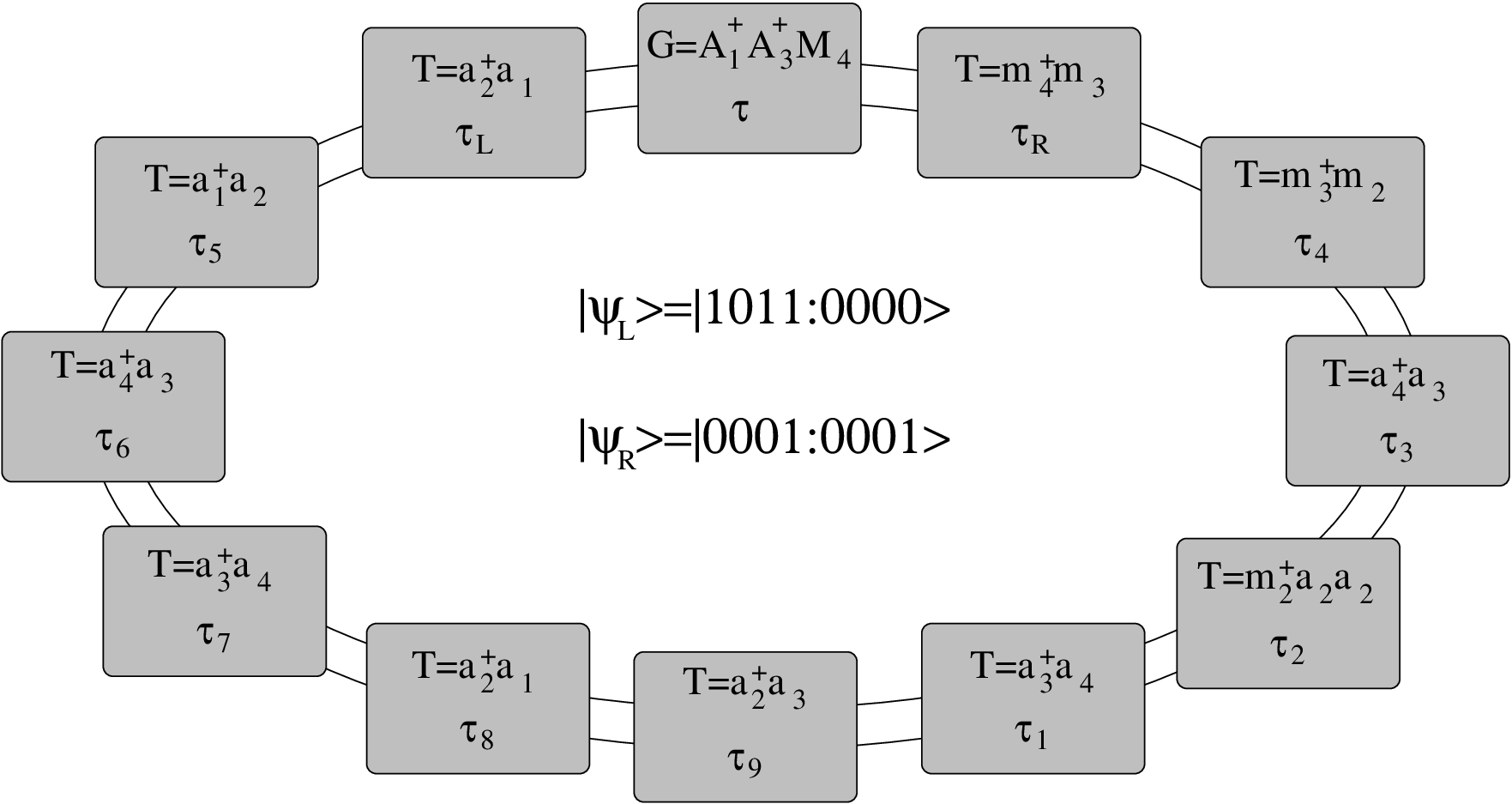
This data structure is part of a doubly linked list. It can be used to build the operator string by linking the ”Operators” together. The states $\big|\psi_{L}\big\rangle$ and $\big|\psi_{R}\big\rangle$ can be represented by arrays of occupation numbers. The configuration of the operator string is then fully represented (Fig. 3). This structure has the advantage to allow easily the insertion of a new piece or the destruction of a piece, which correspond respectively to a creation or a destruction of a $\hat{\mathcal{T}}$ operator. Changing the time $\tau$ of the Green operator in the range $\big[\tau_{L},\tau_{R}\big]$ corresponds to moving the Green operator between its left and right $\hat{\mathcal{T}}$ operators.

It is useful here to add some extra information in the computer. We define the ”Field operator” data structure in order to have a suitable representation of the Green operator:

•

Type – An integer describing the type of the normalized field operator, $A_{i}^{\dagger}$ , $A_{i}^{\phantom{\dagger}}$ , $M_{i}^{\dagger}$ , or $M_{i}^{\phantom{\dagger}}$ .
•

Index – An integer describing the site index where the field operator is acting.
•

Ptr – A pointer onto a ”Field operator” data structure that represents the next field operator.

This data structure is part of a linked list. It can be used to build the term of the Green operator that connects the states $\big|\psi_{L}\big\rangle$ and $\big|\psi_{R}\big\rangle$ (Fig. 4). We will call this term the ”active term” of $\hat{\mathcal{G}}$ and denote it by $G$ .

We have seen in section III.C that we need to be able to evaluate matrix elements of the form:

	$\displaystyle\!\!\!\!\!\!N_{T}=\big\langle\psi_{k+1}\big\|\hat{\mathcal{T}}\big\|\psi_{k}\big\rangle$		(89)
	$\displaystyle\!\!\!\!\!\!N_{G}=\big\langle\psi_{L}\big\|\hat{\mathcal{G}}\big\|\psi_{R}\big\rangle$		(90)
	$\displaystyle\!\!\!\!\!\!N_{GT}=\big\langle\psi_{L}\big\|\hat{\mathcal{G}}\hat{\mathcal{T}}\big\|\psi_{R}\big\rangle=\sum_{\psi}\big\langle\psi_{L}\big\|\hat{\mathcal{G}}\big\|\psi\big\rangle\big\langle\psi\big\|\hat{\mathcal{T}}\big\|\psi_{R}\big\rangle$		(91)
	$\displaystyle\!\!\!\!\!\!N_{TG}=\big\langle\psi_{L}\big\|\hat{\mathcal{T}}\hat{\mathcal{G}}\big\|\psi_{R}\big\rangle=\sum_{\psi}\big\langle\psi_{L}\big\|\hat{\mathcal{T}}\big\|\psi\big\rangle\big\langle\psi\big\|\hat{\mathcal{G}}\big\|\psi_{R}\big\rangle$		(92)

The $N_{T}$ matrix element is easy to calculate, since we know from the ”Operator” data structure which term of $\hat{\mathcal{T}}$ is acting. The $N_{G}$ matrix element is also easy to calculate: We just run over the linked list that represents the active term of the Green operator and count how many creation operators and how many annihilation operators we have. The value of the matrix element is then given by the $g_{pq}$ matrix.

The evaluation of the $N_{GT}$ (or $N_{TG}$ ) matrix element is required when we calculate the probability of insertion of a new $\hat{\mathcal{T}}$ operator. For this, we need to look for all possible intermediate states $\big|\psi\big\rangle$ . For a given intermediate state, only one term of the $\hat{\mathcal{T}}$ operator (for example $a_{3}^{\dagger}a_{4}^{\phantom{\dagger}}$ or $m_{2}^{\dagger}a_{2}^{\phantom{\dagger}}a_{2}^{\phantom{\dagger}}$ ) gives a non-zero value to the matrix element. We will call this term the ”active term” of $\hat{\mathcal{T}}$ and denote it by $\tilde{T}$ . The important thing to notice is that all active terms are inversible and that the inverse of $\tilde{T}$ is proportional to $\tilde{T}^{\dagger}$ . So the procedure is the following: Instead of building the list of states that we get by applying $\hat{\mathcal{T}}$ onto $\big|\psi_{R}\big\rangle$ for $N_{GT}$ (or $\big\langle\psi_{L}\big|$ for $N_{TG}$ ), we build a list of all possible active terms $\tilde{T}$ that give a non zero value when applied onto the ket (or the bra). Then for each possible active term $\tilde{T}$ we consider the associated normalized operator $T$ (obtained by replacing all creation and annihilation operators by the corresponding normalized operators (11)), and we build the new corresponding active term $G^{\>\prime}$ of the Green operator as folows:

	$\displaystyle\big\langle\psi_{L}\big\|\hat{\mathcal{G}}\big\|\psi_{R}\big\rangle\rightarrow\big\langle\psi_{L}\big\|\hat{\mathcal{G}}\big\|\psi\big\rangle\big\langle\psi\big\|\hat{\mathcal{T}}\big\|\psi_{R}\big\rangle$
	$\displaystyle\Rightarrow G^{\>\prime}=GT^{\dagger}$		(93)
	$\displaystyle\big\langle\psi_{L}\big\|\hat{\mathcal{G}}\big\|\psi_{R}\big\rangle\rightarrow\big\langle\psi_{L}\big\|\hat{\mathcal{T}}\big\|\psi\big\rangle\big\langle\psi\big\|\hat{\mathcal{G}}\big\|\psi_{R}\big\rangle$
	$\displaystyle\Rightarrow G^{\>\prime}=T^{\dagger}G$		(94)

It is clear that equations (93) and (94) always have a solution for $G^{\>\prime}$ , and that it corresponds to a term of the Green operator. This ensures that it is always possible to create a $\hat{\mathcal{T}}$ operator acting on any state at any imaginary time. It may happen that the new active term $G^{\>\prime}$ contains normalized creation and annihilation operators that cancel each other. In that case a ”simplification procedure” has to be called in order to remove the obsolete operators and prevent a useless growing of the linked list. Having determined all new $(G^{\>\prime},\tilde{T})$ pairs, it is easy to calculate the weights of the corresponding matrix elements. Then a particular pair can be chosen with a probability proportional to its weight. A new piece of ”Operator” data structure is then created and initialized with the active term $\tilde{T}$ of the chosen pair, and inserted in the doubly linked list of the operator string. The active term $G$ of the Green operator is also updated with $G^{\>\prime}$ .

Finally, we need to determine the new active term $G^{\>\prime}$ of the Green operator when a $\hat{\mathcal{T}}$ operator is destroyed. It is simply given by:

	$\displaystyle\big\langle\psi_{L+1}\big\|\hat{\mathcal{T}}\big\|\psi_{L}\big\rangle\big\langle\psi_{L}\big\|\hat{\mathcal{G}}\big\|\psi_{R}\big\rangle\rightarrow\big\langle\psi_{L+1}\big\|\hat{\mathcal{G}}\big\|\psi_{R}\big\rangle$
	$\displaystyle\Rightarrow G^{\>\prime}=TG$		(95)
	$\displaystyle\big\langle\psi_{L}\big\|\hat{\mathcal{G}}\big\|\psi_{R}\big\rangle\big\langle\psi_{R}\big\|\hat{\mathcal{T}}\big\|\psi_{R-1}\big\rangle\rightarrow\big\langle\psi_{L}\big\|\hat{\mathcal{G}}\big\|\psi_{R-1}\big\rangle$
	$\displaystyle\Rightarrow G^{\>\prime}=GT$		(96)

Again, $G^{\>\prime}$ always has a solution which is a particular term of the Green operator. Thus it is always possible to destroy any encountered operator. The ”simplification procedure” is again called in order to remove obsolete normalized creation and annihilation operators in the new $G^{\>\prime}$ . The $\hat{\mathcal{T}}$ operator is removed from the doubly linked list of the operator string, and the active term $G$ of the Green operator is updated with $G^{\>\prime}$ .

As a concrete example, let us build the list of all possible active terms $\tilde{T}$ of the $\hat{\mathcal{T}}$ operator that can be inserted to the left of the Green operator of Fig. 3, and the associated active terms $G^{\>\prime}$ . We look for all possible transitions:

	$\displaystyle\big\langle 1011:0000\big\|\hat{\mathcal{G}}\big\|0001:0001\big\rangle$
	$\displaystyle\quad\rightarrow\big\langle 1011:0000\big\|\hat{\mathcal{T}}\big\|\psi\big\rangle\big\langle\psi\big\|\hat{\mathcal{G}}\big\|0001:0001\big\rangle$		(97)
	$\displaystyle\Rightarrow G^{\>\prime}=T^{\dagger}G$		(98)

The solutions (after simplification of $G^{\>\prime}$ ) are:

\tilde{T}=\left|\begin{array}[]{l}a_{1}^{\dagger}a_{2}^{\phantom{\dagger}}\\ a_{1}^{\dagger}a_{4}^{\phantom{\dagger}}\\ a_{3}^{\dagger}a_{2}^{\phantom{\dagger}}\\ a_{3}^{\dagger}a_{4}^{\phantom{\dagger}}\\ a_{4}^{\dagger}a_{3}^{\phantom{\dagger}}\\ a_{4}^{\dagger}a_{1}^{\phantom{\dagger}}\end{array}\right.\hskip 28.45274ptG^{\>\prime}=\left|\begin{array}[]{l}A_{2}^{\dagger}A_{3}^{\dagger}M_{4}^{\phantom{\dagger}}\\ A_{3}^{\dagger}A_{4}^{\dagger}M_{4}^{\phantom{\dagger}}\\ A_{2}^{\dagger}A_{3}^{\dagger}M_{4}^{\phantom{\dagger}}\\ A_{1}^{\dagger}A_{4}^{\dagger}M_{4}^{\phantom{\dagger}}\\ A_{1}^{\dagger}A_{3}^{\dagger}A_{3}^{\dagger}A_{4}^{\phantom{\dagger}}M_{4}^{\phantom{\dagger}}\\ A_{1}^{\dagger}A_{1}^{\dagger}A_{3}^{\dagger}A_{4}^{\phantom{\dagger}}M_{4}^{\phantom{\dagger}}\end{array}\right.

(99)

Let us suppose that the $(\tilde{T}=a_{4}^{\dagger}a_{1},G^{\>\prime}=A_{1}^{\dagger}A_{1}^{\dagger}A_{3}^{\dagger}A_{4}M_{4})$ pair is chosen. The new state $\big|\psi\big\rangle$ introduced on the left of the Green operator is:

	$\displaystyle\big\|\psi\big\rangle$	$\displaystyle=$	$\displaystyle A_{1}^{\dagger}A_{1}^{\dagger}A_{3}^{\dagger}A_{4}M_{4}\big\|0001:0001\big\rangle$		(100)
		$\displaystyle=$	$\displaystyle\big\|2010:0000\big\rangle$		(100)

Now if we decide to destroy the $\hat{\mathcal{T}}$ operator on the right of the Green operator, the state $\big|\psi_{R}\big\rangle$ is removed and the only solution for the new active term $G^{\>\prime\prime}$ is (after simplification):

	$\displaystyle G^{\>\prime\prime}$	$\displaystyle=$	$\displaystyle G^{\>\prime}M_{4}^{\dagger}M_{3}$		(101)
		$\displaystyle=$	$\displaystyle A_{1}^{\dagger}A_{1}^{\dagger}A_{3}^{\dagger}A_{4}M_{3}$		(101)

The new state $\big|\psi_{R}^{\prime}\big\rangle$ on the right of the Green operator is given by:

	$\displaystyle\big\|\psi_{R}^{\prime}\big\rangle$	$\displaystyle=$	$\displaystyle M_{3}^{\dagger}M_{4}\big\|\psi_{R}\big\rangle$		(102)
		$\displaystyle=$	$\displaystyle\big\|0001:0010\big\rangle$		(102)

This example illustrates how the algorithm is easy to apply to any Hamiltonian of the form (1), provided that the non-diagonal part $\hat{\mathcal{T}}$ is positive definite. Figures 5 and 6 show a comparison between an exact diagonalization on a 4-site lattice initially loaded with 3 atoms and no molecule, and QMC results obtained with the SGF algorithm. The perfect agreement confirms the exactness of the algorithm.

V Conclusion

We present a new quantum Monte Carlo algorithm: The Stochastic Green Function algorithm. This algorithm can be easily applied to a wide class of Hamiltonians, including multi-species Hamiltonians. The algorithm is completely independent of the dimension of the system, and works in the canonical ensemble, which is prefered for systems with several species of particles. Finally, the algorithm gives access to n-body Green functions, which provide momentum distribution functions, thus allowing useful connections with experiments.

Acknowledgements.

I thank Peter Denteneer for useful conversations and suggestions. This work is part of the research program of the ’Stichting voor Fundamenteel Onderzoek der materie (FOM)’, which is financially supported by the ’Nederlandse Organisatie voor Wetenschappelijk Onderzoek (NWO)’. I would like to thank my fiancée Salima Zine for allowing me to work on week-ends.

References

(1) M. Rigol and A. Muramatsu, Phys. Rev. A 69, 053612 (2004).
(2) M. Rigol, A. Muramatsu, G. G. Batrouni, and R. T. Scalettar, Phys. Rev. Lett. 91, 130403 (2003).
(3) R. Blankenbecler, R.L. Sugar, and D.J. Scalapino, Phys. Rev. D 24, 2278 (1981).
(4) S.R. White, D.J. Scalapino, R.L. Sugar, N.E. Bickers, and R.T. Scalettar, Phys. Rev. B 39, 839 (1989).
(5) G.G. Batrouni, R.T. Scalettar, and G.T. Zimanyi, Phys. Rev. Lett. 65, 176 (1990).
(6) G.G. Batrouni and R.T. Scalettar, Phys. Rev. B 46, 9051 (1992).
(7) A.W. Sandvik, J. Phys. A 25, 3667 (1992); Phys. Rev. B 59, 14157 (1999).
(8) N.V. Prokof’ev, B.V. Svistunov, and I.S. Tupitsyn, JETP Lett. 87, 310 (1998).
(9) V.G. Rousseau, R.T. Scalettar, and G.G. Batrouni, Phys. Rev. B 72, 054524 (2005).
(10) K. Van Houcke, S. M. A. Rombouts, and L. Pollet, Phys. Rev. E 73,056703 (2006).
(11) S. M. A. Rombouts, K. Van Houcke, and L. Pollet, Phys. Rev. Lett. 96, 180603 (2006).
(12) V.G. Rousseau and P.J.H. Denteneer, Phys. Rev. A 77, 013609 (2008).
(13) E. Timmermans, P. Tommasini, M. Hussein, and A. Kerman, Physics Reports 315, 199 (1999).
(14) K. Sengupta and N. Dupuis, Europhys. Lett. 70, 586 (2005).
(15) L. Pollet, M. Troyer, K. Van Houcke, and S.M.A. Rombouts, Phys. Rev. Lett. 96, 190402 (2006).
(16) P. Sengupta and L.P. Pryadko, Phys. Rev. B 75, 132507 (2007).
(17) F. Hébert, F. Haudin, L. Pollet, and G.G. Batrouni, Phys. Rev. A 76, 043619 (2007).
(18) N. Metropolis, A.W. Rosenbluth, M.N. Metropolis, A.H. Teller, and E. Teller, J. Chem. Phys. 21, 1087 (1953).
(19) E.L. Pollock, and D.M. Ceperley, Phys. Rev. B 36, 8343 (1987).
(20) D. Heidarian and S. Sorella, Phys. Rev. B 75, 241104 (2007).

	$\displaystyle\!\!\!\!\!\!\!\mathcal{Z}(\beta,\tau)\!\!=\!\!\!\sum\int_{0<\tau_{1}<\cdots<\tau_{n}<\beta}\hskip-56.9055pt\big\langle\psi_{0}\big\|e^{-\beta\mathcal{V}}\hat{\mathcal{T}}(\tau_{n})\big\|\psi_{n-1}\big\rangle\big\langle\psi_{n-1}\big\|\hat{\mathcal{T}}(\tau_{n-1})\big\|\psi_{n-2}\big\rangle$
	$\displaystyle\!\!\!\!\!\!\!\times\cdots\big\langle\psi_{L+1}\big\|\hat{\mathcal{T}}(\tau_{L})\big\|\psi_{L}\big\rangle\big\langle\psi_{L}\big\|\hat{\mathcal{G}}(\tau)\big\|\psi_{R}\big\rangle\big\langle\psi_{R}\big\|\hat{\mathcal{T}}(\tau_{R})\big\|\psi_{R-1}\big\rangle$		(9)
	$\displaystyle\!\!\!\!\!\!\!\times\cdots\big\langle\psi_{2}\big\|\hat{\mathcal{T}}(\tau_{2})\big\|\psi_{1}\big\rangle\big\langle\psi_{1}\big\|\hat{\mathcal{T}}(\tau_{1})\big\|\psi_{0}\big\rangle d\tau_{1}\cdots d\tau_{n}$

The Stochastic Green Function (SGF) algorithm

Abstract

pacs

I Introduction

II Motivations

III The algorithm

III.1 The partition function and the ”Green operator”

III.2 The update scheme

III.3 Detailed balance

III.3.1 No creation, shift, no destruction

III.3.2 Creation, shift, no destruction

III.3.3 No creation, shift, destruction

III.3.4 Creation, shift, destruction

III.3.5 Simplification of the acceptance factors

III.3.6 Determination of the gp​qg_{pq} matrix

III.3.7 Efficiency and purposes of the algorithm

III.4 Measuring physical quantities

III.4.1 Quantities represented by diagonal operators

III.4.2 Quantities represented by non-diagonal operators

III.5 Improved estimator for the zero-temperature superfluid density

IV The algorithm in practice

V Conclusion

Acknowledgements.

References

III.3.6 Determination of the $g_{pq}$ matrix