Perfect fluid quantum Universe in the presence of negative cosmological constant
Abstract
We present perfect fluid Friedmann-Robertson-Walker quantum cosmological models in the presence of negative cosmological constant. In this work the Schutz’s variational formalism is applied for radiation, dust, cosmic string, and domain wall dominated Universes with positive, negative, and zero constant spatial curvature. In this approach the notion of time can be recovered. These give rise to Wheeler-DeWitt equations for the scale factor. We find their eigenvalues and eigenfunctions by using Spectral Method. After that, we use the eigenfunctions in order to construct wave packets for each case and evaluate the time-dependent expectation value of the scale factors, which are found to oscillate between finite maximum and minimum values. Since the expectation values of the scale factors never tends to the singular point, we have an initial indication that these models may not have singularities at the quantum level.
Pacs:98.80.Qc, 04.40.Nr, 04.60.Ds
1 Introduction
Quantum cosmological models are important subjects on the interface of cosmology and gravitation. At first, B. DeWitt [1] quantized a Friedmann Universe filled with dust and later, closed isotropic cosmological models with matter as a conformal and minimally coupled scalar fields were quantized [2, 3]. Misner worked on the quantization of anisotropic cosmological models [4], and Barabanenkov quantized the Friedmann metric matched with the Kruskal one [5]. The quantization of a dust-like closed isotropic cosmological model with a cosmological constant is also investigated in Ref. [6].
In the quantum cosmology the Wheeler-DeWitt (WD) equation which determines the wave function of the Universe, can be constructed using ADM decomposition of the geometry [7] in the Hamiltonian formalism of general relativity. However, quantum cosmology has many technical and conceptual problems. In fact, the WD equation of quantum gravity is a functional differential equation defined in the superspace which is the space of all possible three dimensional spatial metrics, and no general solution is known in this superspace. In quantum cosmology this problem is avoided by using symmetry requirements to freeze out an infinite number of degrees of freedom, leaving only a few for quantization process. This procedure defines a minisuperspace, where exact solutions can often be found. On the other hand, the general covariance will be lost upon applying the ADM decomposition, and in most cases the notion of time disappears at the quantum level [8]. Even, if all these problems are solved, the interpretation of the central object, i.e. the wave function of the Universe, remains unanswered.
The many-worlds interpretations [9] of quantum mechanics is one of the most popular interpretation schemes for the wave function of the Universe. This interpretation differs noticeably from the Copenhagen interpretation of quantum mechanics since the conception of probability is abandoned in some sense. In fact, all possibilities are participated to create new Universes with different possible eigenvalues obtained by measurements. The evolution of observables such as scale factor is found by evaluating the expectation values. In this case, like in the Copenhagen interpretation, the structure of Hilbert space and self-adjoint operators are still unchanged.
The presence of the matter in quantum cosmology needs further consideration and can be described by fundamental fields, as done in Ref. [10]. Using WKB approximation one can predict the behavior of the quantum Universe which leads to determination of the trajectories in phase space. However, even in the minisuperspace, general exact solutions are hard to find, the Hilbert space structure is ambiguous and it is difficult to recover the conception of a semiclassical time [8, 10].
Here, we consider matter as a perfect fluid. This description is basically semiclassical, but it introduces a variable, which can be identified with time and connected with the matter degrees of freedom, leading to a well-defined Hilbert space structure. Moreover, this allow us to treat the barotropic equation of state with arbitrary .
It is very convenient to construct a quantum perfect fluid model. Schutz’s formalism [11, 12] gives dynamics to the fluid degrees of freedom in interaction with the gravitational field. Using a proper canonical transformations, at least one conjugate momentum operator associated with matter appears linearly in the action integral. Therefore, a Schrödinger-like equation can be obtained where the matter plays the role of time. Moreover, recently, some applications of the Schutz’s formalism have been discussed in the framework of the perfect fluid Stephani Universe [13, 14] and Friedmann-Robertson-Walker (FRW) Universe in the presence of Chaplygin gas [15, 16].
Until now, quantum perfect fluid models with common equations of state have been constructed in the absence of cosmological constants [17, 18, 19, 20, 21]. We can study the behavior of the scale factor using the many-worlds and the de Broglie-Bohm interpretations of quantum mechanics.
Recently, the quantization of FRW radiation dominated Universe in the presence of a negative cosmological constant is discussed by Monerat et al [22]. However, as mentioned in Ref. [23], their results are inaccurate and their relative errors range between for the ground state of case, and for the ground state of , which make their work unreliable. Here, we generalize the previous investigations by studying quantum perfect fluid models for barotropic equation of state , where correspond to radiation, dust, cosmic string, and domain wall dominated Universes, respectively. Using the many-worlds framework, the behavior of the scale factor is determined, although the results are independent of the interpretation scheme employed. The large time average of the expectation value of the scale factor is similar to the classical case. Moreover, the model predicts an accelerated expansion today if .
It is important to mention that although recent observations point toward a positive cosmological constant, it is still possible that at the very early Universe the cosmological constant be negative. Moreover, we think it is important to understand more about such models which represent bound Universes.
This paper is organized as follows. We quantize three Friedmann-Robertson-Walker perfect fluid models in the presence of a negative cosmological constant, using the formalism of quantum cosmology. In Sec. 2, the quantum cosmological model with a perfect fluid as the matter content is constructed in Schutz’s formalism [11, 12], and the WD equation in minisuperspace is Found to quantize the model. The wave-function depends on the scale factor and on the canonical variable associated to the fluid which plays the role of time , in the Schutz’s variational formalism. We separate the wave-function in two parts, one depending solely on the scale factor and the other depending only on the time. The solution in the time sector of the WD equation is trivial, leading to imaginary exponentials of the type , where is the system energy and . In Sec. 3, we outline the Spectral Method [24, 25, 26], and use it to find the eigenvalues and eigenfunctions of corresponding WD equations. In Sec. 4, we construct wave packets from the eigenfunctions, for radiation, dust, cosmic string and domain wall dominated Universes respectively, and compute the time-dependent expectation values of the scale factors for . In Sec. 5, we state our conclusions.
2 Model
Let us start from the Einstein-Hilbert action plus a perfect fluid in the formalism developed by Schutz. For this, we write down the action for gravity plus perfect fluid as
| (1) |
here, is the extrinsic curvature, is the cosmological constant, and is the induced metric over the three-dimensional spatial hypersurface, which is the boundary of the four dimensional manifold . We choose units such that the factor becomes equal to one. The first two terms were first obtained in [7] and the last term of (1) represents the matter contribution to the total action, being the pressure which obeys the barotropic equation of state . In Schutz’s formalism [11, 12] the fluid’s four-velocity can be expressed in terms of five potentials , , , and
| (2) |
where is the specific enthalpy. is the specific entropy, and the potentials and are connected with rotation which are absent of models in the FRW type. The variables and have no clear physical meaning. The four-velocity also satisfies the normalization condition
| (3) |
The FRW metric
| (4) |
can be inserted in the action (1), where is the lapse function and is the metric on the constant-curvature spatial section. After some thermodynamical considerations and using the constraints for the fluid, and dropping the surface terms, the final reduced action takes the form [18].
| (5) |
The reduced action may be further simplified using canonical methods [18], resulting in the super-Hamiltonian
| (6) |
where and , being the rest mass density of the fluid. The following additional canonical transformations, which generalizes the one used in [18],
| (7) |
simplifies the super-Hamiltonian to,
| (8) |
where the momentum is the only remaining canonical variable associated with matter and appears linearly in the super-Hamiltonian. The parameter defines the curvature of the spatial section, taking the values for a flat, close or open Universes, respectively.
The classical dynamics is governed by the Hamilton equations, derived from Eq. (8) and Poisson brackets as
| (9) |
We also have the constraint equation . Choosing the gauge , we have the following solutions for the system
| (10) | |||||
| (11) |
The classical equation of motion for the scale factor in absent of the cosmological constant is solved in a unified form for any in terms of hypergeometric functions in Ref. [27]. Moreover, In the radiation dominated Universe () with a negative cosmological constants, the classical solutions have been obtained using Jacobi’s elliptic sine functions [22]. the WD equation in minisuperspace can be obtained by imposing the standard quantization conditions on the canonical momenta and (, ) demanding that the super-Hamiltonian operator annihilate the wave function ()
| (12) |
where corresponds to the time coordinate. Equation (12) takes the form of a Schrödinger equation . Demanding that the Hamiltonian operator to be self-adjoint, the inner product of any two wave functions and must take the form [28, 19]
| (13) |
On the other hand, the wave functions should satisfy the following boundary conditions
| (14) |
The WD equation (12) can be solved by separation of variables as follows
| (15) |
where the dependent part of the wave function () satisfies
| (16) |
Since the energy term grows faster than the potential for , this equation has a discrete spectra () with associated bound state eigenfunctions () only for .
We construct a general solution to the WD equation (12) by taking linear combinations of the ’s,
| (17) |
where the coefficients will be fixed later. Form pure mathematical point of view, by allowing negative values of , the Parity operator can be defined. If the WD equation (Eq. 16) is covariant under the Parity operator, its eigenfunctions can be separated into even and odd ones. The even or odd wave packets constructed from appropriate linear combinations of the eigenstates, have the important property that they will not change their parity in the course of their time evolution. Therefore, if we choose the initial wave packets to be odd or even, that is they satisfy either the first or the second condition stated in Eq. 14 respectively, they will satisfy them for all times. We can compute the expected value for the scale factor for any wave function, using the many worlds interpretation of quantum mechanics. This means, we may write the expected value for the scale factor as [29]
| (18) |
Before solving the WD equation (16) via Spectral Method, it is worthy to state a brief overview of the Chhajlany and Malnev method and Variational Sinc Collocation Method (VSCM), which have been recently used to solve the WD equation (16), for radiation epoch () in Refs. [22, 23], respectively.
In Chhajlany and Malnev method [30, 31], one adds an extra term to the original anharmonic oscillator potential to find a subset of normalizable solutions of the modified Hamiltonian. In the case of equation (16) this extra term is where is constant. Now, the solution can be written as a polynomial where the larger the degree of the polynomial, the smaller the constant, is. In fact, by increasing the order of polynomial, the energy eigenvalues predicted by this method approach monotonically to the energy eigenvalues of the original Hamiltonian.
On the other hand, to obtain highly accurate numerical results, both for the energy eigenvalues and eigenfunctions, one can use Variational Sinc Collocation Method (VSCM) [32]. It is shown that the errors decay exponentially with the number of elements (sinc functions) used for discretization of the Hamiltonian. Diagonalization of the resulting matrix, by specification of the otherwise arbitrary grid spacing (spacing between two contiguous sinc functions), yields energy eigenvalues and eigenfunctions. As shown by Amore et al, for a specified number of sinc functions, there exists an optimal value of which yields the minimum errors [32]. this optimal value can be found using the Principle of Minimal Sensitivity (PMS) [33] to the trace of the Hamiltonian matrix.
As indicated by Lemos et al, the need for a modified potential instead of the original one in the Chhajlany and Malnev method, gives rise to significant errors, particularly for [34]. In fact, VSCM is more uniformly accurate and converges more rapidly than the Chhajlany and Malnev method.
3 The Spectral Method
In this section we introduce Spectral Method (SM) [24, 25] as a tool for solving differential equation. We have recently used the Spectral Method for constructing the appropriate wave packets which are solutions to a WD equation [26]. This method is simple, fast, accurate and stable.
Let us consider the general time-independent WD equation (EQ. (16)),
| (19) |
where and are arbitrary, but with derivative operators less than two. For the usual eigenvalue problem , which includes the time-independent Schrödinger equation. The method SM can be easily extended to solve the general case which is a operator in the space. This generalize problem can be named a generalized eigenvalue problem. Throughout this paper, we only examine the bound states of this problem, i.e. the states which are the square integrable. The configuration space for most physical problems are defined by . Since the bound states fall off sufficiently fast for large , a finite region suffices, and the proper choice for this region, say . The use of a finite domain is also necessary since we need to choose a finite subspace of a countably infinite basis. We find it convenient to shift the domain to . In particular, we need to shift the potential energy functions also. This means that we can expand the solution as,
| (20) |
We can also make the following expansions,
| (21) | |||||
| (22) |
where are coefficients that can be determined once and are specified. By substituting Eqs. (20,21,22) into Eq. (19) and using the differential equation of the Fourier basis we obtain,
| (23) |
Because of the linear independence of , every term in the summation must satisfy,
| (24) |
It only remains to determine the matrices and . Using Eqs. (21,22) and Eq. (20) we have,
| (25) | |||
| (26) |
By multiplying both sides of the above equations by and integrating over the -space and using the orthonormality condition of the basis functions, one finds,
| (27) | |||
| (28) |
where,
| (29) | |||
| (30) |
Therefore we can rewrite Eq. (24) as,
| (31) |
It is obvious that the presence of the operators and in Eq. (19), leads to nonzero coefficients and in Eq. (31), which in principle could couple all of the vector elements of . It is easy to see that the more basis functions we include, the closer our solution will be to the exact one. We select a finite subset of the basis functions i.e. the first ones, by letting the index run from 1 to in the summations. Equation (31) can be written as,
| (32) |
or,
| (33) |
where and are square matrices with elements. Their elements can be obtained from Eq. (31). The solution to this matrix equation simultaneously yields sought after eigenstates and eigenvalues. It is important to note that the optimized value of crucially depends on the number of basis functions (), which results in the maximum accuracy and the stability of the solutions (for a comprehensive study about the optimization procedure see [25]).
4 Results
In this section we will solve the equation (16) using SM. By choosing basis functions, and we report our results with 10 significant digits. Note that, although, we are free to choose other values of , but the accuracy of results for small reduces in comparison with large values of for a given number of basis , particularly for . This means that we need to increase the number of basis to obtain the same accuracy which increases the computations. With regard to these considerations, the results are robust under changes of Lambda.
4.1 Radiation ()
In the radiation dominated Universe time-independent WD equation has the following form,
| (34) |
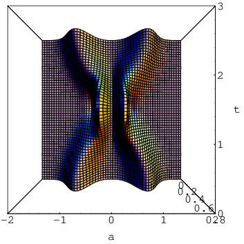
In this form it is obvious that the system is absolutely stable for . Note that equation is covariant under the Parity operator. For ease of comparison of our results with those of Refs. [22, 23], we select the first condition of the equation (14) and choose the coefficients s in equation (17) to be 1 and zero for the odd and even eigenfunctions, respectively. We can find the energy eigenvalues and eigenvectors of this equation with ease using SM where and in comparison with Eq. (19). Table 1 shows the first 26 odd eigenvalues for respectively. Figures (1,2,3) show the resulting expectation values of the scale factor , versus for the various values of . As can be seen from the table, the results are as same as those reported in Ref. [23]. To show the arbitrariness in choosing initial odd wave packet, we can use the coefficients of odd coherent state of the quantum simple harmonic oscillator. Figure 4 shows the 3D plot of resulting wave packet for case.


| 1.510262538 | 0.3364795921 | -21.79569604 | |
| 3.550647291 | 1.031199050 | -20.39848969 | |
| 5.621893706 | 1.880761581 | -19.01885126 | |
| 7.722777814 | 2.842487493 | -17.65745105 | |
| 9.852194220 | 3.894746211 | -16.31503013 | |
| 12.00913857 | 5.024091561 | -14.99241327 | |
| 14.19269339 | 6.221192430 | -13.69052532 | |
| 16.40201655 | 7.479120856 | -12.41041248 | |
| 18.63633173 | 8.792490724 | -11.15327022 | |
| 20.89492047 | 10.15697184 | -9.920481041 | |
| 23.17711552 | 11.56899282 | -8.713666752 | |
| 25.48229516 | 13.02554815 | -7.534763378 | |
| 27.80987836 | 14.52406697 | -6.386132854 | |
| 30.15932069 | 16.06232038 | -5.270738293 | |
| 32.53011067 | 17.63835396 | -4.192437789 | |
| 34.92176669 | 19.25043737 | -3.156519423 | |
| 37.33383429 | 20.89702582 | -2.170719225 | |
| 39.76588373 | 22.57673016 | -1.246288323 | |
| 42.21750793 | 24.28829319 | -0.3899963301 | |
| 44.68832056 | 26.03057067 | 0.4337198672 | |
| 47.17795441 | 27.80251593 | 1.300741394 | |
| 49.68605987 | 29.60316715 | 2.243855391 | |
| 52.21230364 | 31.43163692 | 3.256001774 | |
| 54.75636750 | 33.28710339 | 4.326509414 | |
| 57.31794728 | 35.16880284 | 5.448058248 | |
| 59.89675181 | 37.07602341 | 6.615611361 |
4.2 Dust ()
In dust dominated Universe time-independent WD equation has the following form,
| (35) |
We can find the energy eigenvalues and eigenvectors of this equation with ease using SM where and in notation displayed in Eq. (19). Table 2 shows the first 20 positive eigenvalues for respectively. Note that, for any positive eigenvalues (), there is an negative counterpart () which . The above equation, is not invariant under the Parity operator. Therefore, its eigenfunctions can not in general satisfy either of the conditions of equation (14. However, we can construct wave packets, from linear combinations of the eigenfunctions, which vanishes at and . Then we need to check that the constraints (Eq. 14 remain valid for all for our choice of initial condition. For example we can choose the coefficients s so as to construct a gaussian initial wave packet () which is centered e.g. at . Figures (5,6,7) show the resulting expectation values of the scale factor , versus for the various values of . As can seen from the figures these wave packets always satisfy the first boundary condition (Eq. 14).
In the case , the time-independent WD equation (35) reduces to
| (36) |
In terms of the new variable we find
| (37) |
Equation (37) is formally identical to the time-independent Schrödinger equation for a harmonic oscillator with unit mass and energy :
| (38) |
where and . Therefore, the allowed values of are and the possible values of are
| (39) |
Thus the stationary solutions are
| (40) |
where
| (41) |
and are the -th Hermite polynomial.


| 4.660967538 | 3.354101966 | 1.955113416 | |
| 11.92641527 | 10.06230590 | 8.159825054 | |
| 18.98089410 | 16.77050983 | 14.53079652 | |
| 25.95270272 | 23.47871376 | 20.97932418 | |
| 32.87827896 | 30.18691770 | 27.47251428 | |
| 39.77369328 | 36.89512163 | 33.99515040 | |
| 46.64761142 | 43.60332556 | 40.53888200 | |
| 53.50529876 | 50.31152949 | 47.09859109 | |
| 60.35022067 | 57.01973343 | 53.67089213 | |
| 67.18479286 | 63.72793736 | 60.25341729 | |
| 74.01077406 | 70.43614129 | 66.84443864 | |
| 80.82948903 | 77.14434522 | 73.44265237 | |
| 87.64196335 | 83.85254916 | 80.04704775 | |
| 94.44900906 | 90.56075309 | 86.65682363 | |
| 101.2512814 | 97.26895702 | 93.27133299 | |
| 108.0493176 | 103.9771610 | 99.89004490 | |
| 114.8435643 | 110.6853649 | 106.5125177 | |
| 121.6343972 | 117.3935688 | 113.1383797 | |
| 128.4221359 | 124.1017728 | 119.7673145 | |
| 135.2070546 | 130.8099767 | 126.3990507 | |
| 141.9893905 | 137.5181806 | 133.0333530 |
4.3 Cosmic Strings ()
In Cosmic Strings dominated Universe time-independent WD equation has the following form,
| (42) |
This differential equation is covariant under parity operator and hence its eigenstates can be separated into even and odd ones. We can find the energy eigenvalues and eigenvectors of this equation with ease using SM where and in comparison with Eq. (19). Table 3 shows the first 20 eigenvalues for respectively. By choosing the first condition of the equation (14), the resulting wave packets should consist of only the odd eigenfunctions. Therefore, the coefficients s in equation (17) are arbitrary for the odd eigenfunctions zero for the even ones. To be able to extend the results of Refs. [22, 23] for the radiation case to the present one, we choose the same initial state as their’s. That is the odd ones are all chosen to be equal to one. Figures (8,9,10) show the resulting expectation values of the scale factor , versus for the various values of .


| 11.63722935 | 8.637229353 | 5.637229353 | |
| 19.36451595 | 16.36451595 | 13.36451595 | |
| 25.54276474 | 22.54276474 | 19.54276474 | |
| 30.96152618 | 27.96152618 | 24.96152618 | |
| 35.89633715 | 32.89633715 | 29.89633715 | |
| 40.48441592 | 37.48441592 | 34.48441592 | |
| 44.80660320 | 41.80660320 | 38.80660320 | |
| 48.91557892 | 45.91557892 | 42.91557892 | |
| 52.84808309 | 49.84808309 | 46.84808309 | |
| 56.63102596 | 53.63102596 | 50.63102596 | |
| 60.28486358 | 57.28486358 | 54.28486358 | |
| 63.82560554 | 60.82560554 | 57.82560554 | |
| 67.26607937 | 64.26607937 | 61.26607937 | |
| 70.61676389 | 67.61676389 | 64.61676389 | |
| 73.88635930 | 70.88635930 | 67.88635930 | |
| 77.08218981 | 74.08218981 | 71.08218981 | |
| 80.21050097 | 77.21050097 | 74.21050097 | |
| 83.27676241 | 80.27676241 | 77.27676241 | |
| 86.28668819 | 83.28668819 | 80.28668819 | |
| 89.25169642 | 86.25169642 | 83.25169642 |
4.4 Domain Walls ()
In Domain Walls dominated Universe () the time-independent WD equation has the following form,
| (43) |
We can find the energy eigenvalues and eigenvectors of this equation with ease using SM where and in comparison with Eq. (19). Table 4 shows the first 20 eigenvalues for respectively. Note that, for any positive eigenvalues (), there is an negative counterpart () which . This case is similar to the Dust case and in particular its differential equation is not covariant under Parity Operator and therefore, its eigenfunctions can not in general satisfy either of the conditions stated in equation (14. However, we can construct wave packets, from linear combinations of the eigenfunctions, which vanishes at and . Then we need to check that the constraints (Eq. 14 remain valid for all for our choice of initial condition. For example we can choose the coefficients s so as to construct a gaussian initial wave packet () which is centered e.g. at . Figures (11,12,13) show the resulting expectation values of the scale factor , versus for the various values of . As can seen from the figures these wave packets always satisfy the first boundary condition (Eq. 14).


| 17.07778092 | 12.54649750 | 7.458961879 | |
| 21.41791925 | 18.18718412 | 14.81583000 | |
| 24.32147857 | 21.57780684 | 18.75859852 | |
| 26.60465935 | 24.14422756 | 21.63352524 | |
| 28.52359398 | 26.25664404 | 23.95258205 | |
| 30.19749314 | 28.07460050 | 25.92257362 | |
| 31.69296487 | 29.68328712 | 27.64978790 | |
| 33.05153398 | 31.13420271 | 29.19682156 | |
| 34.30107228 | 32.46114131 | 30.60396527 | |
| 35.46131513 | 33.68761746 | 31.89883581 | |
| 36.54683096 | 34.83073057 | 33.10127373 | |
| 37.56911074 | 35.90336205 | 34.22606529 | |
| 38.54199370 | 36.91577767 | 35.28463557 | |
| 39.50080454 | 37.87984925 | 36.28735433 | |
| 40.512127 | 38.825301 | 37.253593 | |
| 41.627809 | 39.812705 | 38.232631 | |
| 42.859939 | 40.895275 | 39.288909 | |
| 44.203790 | 42.088418 | 40.454402 | |
| 45.653137 | 43.388462 | 41.730668 | |
| 47.203213 | 44.789203 | 43.111449 |
It is important to note that we have repeated the simulations for all cases () with other values of and different initial conditions (subject to ). In particular, we have also repeated simulations for rather than which studied in detail, and found the corresponding eigenvalues and eigenfunctions with desired accuracy. Moreover, we chose other initial conditions in the form with various choices of (), (), and (). We found that, for all these cases the behavior of the expectation value of the scale factor is similar to ones depicted in Figs. 1 to 13 and never tends to the singular point.
5 Conclusions
In this work we have investigated closed, flat, and open minisuperspace FRW quantum cosmological models () with perfect fluid for the radiation, dust, cosmic strings, and domain walls dominated Universes (, respectively). The use of Schutz’s formalism for perfect fluids allowed us to obtain a Schrödinger-like WD equation in which the only remaining matter degree of freedom plays the role of time. We have used Spectral Method and obtained accurate results for the eigenfunctions and eigenvalues. Physically acceptable wave packets were constructed by appropriate linear combination of these eigenfunctions. The time evolution of the expectation value of the scale factor has been determined in the spirit of the many-worlds interpretation of quantum cosmology. Since the expectation values of the scale factors for the cases considered here never tend to the singular point, we have an initial indication that these models may not have singularities at the quantum level. The similar conclusions have been obtained on general grounds in [18] and for the radiation case in [22].
Acknowledgements
Authors thank H. R. Sepangi for useful discussions and comments.
References
- [1] B. S. DeWitt, Phys. Rev. 160, 1113 (1967).
- [2] V. N. Melnikov and V. A. Reshetov, in: Abstr. 8 All-Union Conference on Elementary Particles (Uzhgorod). Kiev, ITP, 117 (1971).
- [3] Yu. N. Barabanenkov and V. A. Pilipenko, in: Abstr. 8 All-Union Conference on Elementary Particles (Uzhgorod). Kiev, ITP, 117 (1971).
- [4] C. W. Misner, Phys. Rev. 186, 1419 (1969).
- [5] Yu. N. Barabanenkov, in: Abstr. 3 Soviet Gravitational Conference, Yerevan (1972).
- [6] M. I. Kalinin, V. N. Melnikov, Grav. Cosmol. 9, 227 (2003).
- [7] R. Arnowitt, S. Deser and C. W. Misner, Gravitation: An Introduction to Current Research, edited by L. Witten, Wiley, New York (1962).
- [8] C. J. Isham, Canonical quantum gravity and the problem of time, arXiv:gr-qc/9210011.
- [9] F. J. Tipler, Phys. Rep. 137, 231 (1986).
- [10] C. Kiefer, Phys. Rev. D 38, 1761 (1988).
- [11] B. F. Schutz, Phys. Rev. D 2, 2762 (1970).
- [12] B. F. Schutz, Phys. Rev. D 4, 3559 (1971).
- [13] P. Pedram, S. Jalalzadeh and S. S. Gousheh, Phys. Lett. B 655, 91 (2007), arXiv:0708.4143.
- [14] P. Pedram, S. Jalalzadeh and S. S. Gousheh, Class. Quantum Grav. 24, 5515 (2007), arXiv:0709.1620.
- [15] P. Pedram, S. Jalalzadeh and S. S. Gousheh, Int. J. Theor. Phys. doi:10.1007/s10773-007-9436-9, arXiv:0705.3587.
- [16] P. Pedram and S. Jalalzadeh, Phys. Lett. B (2007), doi: 10.1016/j.physletb.2007.11.013, arXiv:0705.3587.
- [17] M. J. Gotay and J. Demaret, Phys. Rev. D 28, 2402 (1983).
- [18] V. G. Lapchinskii and V. A. Rubakov, Theor. Math. Phys. 33, 1076 (1977).
- [19] F. G. Alvarenga and N. A. Lemos, Gen. Rel. Grav. 30, 681 (1998).
- [20] J. Acacio de Barros, N. Pinto-Neto and M. A. Sagioro-Leal, Phys. Let. A 241, 229 (1998).
- [21] F. G. Alvarenga, J. C. Fabris, N. A. Lemos, G. A. Monerat, Gen. Rel. Grav. 34, 651 (2002).
- [22] G. A. Monerat, E. V. C. Silva, G. Oliveira-Neto, L. G. F. Filho, and N. A. Lemos, Phys. Rev. D 73, 044022 (2006).
- [23] P. Amore, A. Aranda, M. Cervantes, J. L. Dìaz-Cruz, Francisco M. Fernàndez, Phys. Rev. D 75, 068503 (2007), arXiv:gr-qc/0611029.
- [24] J. P. Boyd, Chebyshev and Fourier Spectral Methods, second ed., Dover, New York, (2001).
- [25] P. Pedram, M. Mirzaei, S. S. Gousheh, arXiv:math-ph/0611008.
- [26] P. Pedram, M. Mirzaei, S.S. Gousheh, Comput. Phys. Commun. 176, 581 (2007).
- [27] M. J. Assad and J. A. S. Lima, Gen. Rel. Grav. 20, 527 (1988).
- [28] N. A. Lemos, J. Math. Phys. 37, 1449 (1996).
- [29] H. Everett, III, Rev. Mod. Phys. 29, 454 (1957).
- [30] S. C. Chhajlany and V. N. Malnev, Phys. Rev. A 42, 3111 (1990).
- [31] S. C. Chhajlany, D. A. Letov, and V. N. Malnev, J. Phys. A 24, 2731 (1991).
- [32] P. Amore, J. Phys. A 39, L349 (2006).
- [33] P. M. Stevenson, Phys. Rev. D 23, 2916 (1981).
- [34] N. A. Lemos, G. A. Monerat, E. V. C. Silva, G. Oliveira-Neto, and L. G. Ferreira Filho, Phys. Rev. D 75, 068504 (2007).