Geometrodynamical Distances to the Galaxy’s Hydrogen Streams
Abstract
We present a geometrodynamical method for determining distances to orbital streams of HI gas in the Galaxy. The method makes use of our offset from the Galactic centre and assumes that the gas comprising the stream nearly follows a planar orbit about the Galactic centre. We apply this technique to the Magellanic Stream and determine the distances to all points along it; a consistency check shows that the angular momentum is approximately constant. Applying this technique to the Large Magellanic Cloud itself gives an independent distance which agrees within its accuracy of around 10%. Relaxing the demand for exact conservation of energy and angular momentum at all points along the stream allows for an increase in orbital period between the lagging end and the front end led by the Magellanic Clouds. Similar methods are applicable to other long streams of high-velocity clouds, provided they also nearly follow planar orbits; these would allow otherwise unknown distances to be determined.
Keywords:
galaxies: Magellanic Clouds — ISM: clouds, kinematics and dynamics — methods: analytical1 Introduction
High-velocity clouds (HVCs) are defined as HI gas which have anomalous velocities that are incompatible with what is expected from a simple Galactic rotation model. Ever since their discovery by Muller et al. 1963, their role in the formation and evolution of our Galaxy has been a source of speculation. Amongst the attempts to explain their origin, the two most well-known and contested are the Galactic Fountain model, in which gas is either being thrown out of the Galactic disk from supernovae or being heated and ionized by massive stars, and the alternative model in which the clouds are pockets of neutral hydrogen left over from the formation epoch of the Galaxy, and which are only now being accreted.
Given the vast sky-coverage of HVCs, the two theories are not necessarily contradictory, as it is likely that some clouds belong to each model. However, with the exception of those HVCs that are obvious components of a stream with a known progenitor, such as the Magellanic (Mathewson et al. 1974) and Sagittarius streams (Putman et al. 2004), the lack of distance measurements has hindered the progress in understanding the role that HVCs play in the Galaxy.
Since newly accreted gas would have a lower metallicity than recycled gas from the Galaxy, metallicity measurements, if available, should be able to distinguish the applicability of each theory on a cloud-by-cloud basis (Sembach et al. 2002; van Woerden et al. 2000; Wakker 2001, e.g.), but it would still be instructive to know exactly where these clouds lie. Observationally, the difficulty in determining direct distances arises from the fact that most of the HVCs do not host stars. If, however, there is one star behind and another to the front of the cloud along the line of sight, both of which have known distances, then a distance bracket can be set for the HVC. The high resolution spectrum of a star directly behind the HVC will exhibit absorption lines at the velocity of that cloud; features that will be absent in the spectrum of a star to the front of the cloud. Starting with the first such measurement for Complex M in the early 90’s (Danly et al. 1993), other HVC complexes for which a distance bracket that now exists include Complex A (Wakker 2001) and Complex WB (Thom et al. 2006). The high latitudes of much of the neutral hydrogen gas in question means there is a lack of background stars bright enough for high resolution spectroscopy, so this technique has not been without difficulty.
Many detailed simulations of streams such as the Magellanic Stream exist (Connors et al. 2006; Mastropietro et al. 2005; Gardiner & Noguchi 1996; Fujimoto & Murai 1985; Fujimoto & Sofue 1976, e.g.), however, all such simulations have many parameters which must be tweaked to give the best fits to the data. In this paper, we describe an alternative set of methods with the aim of probing the elusive distances to streams of HI gas comprising the HVCs. These methods instead make strong hypotheses that enable us to attempt to read the distances out of the data themselves; the studies presented here are neither simulations nor attempts at modelling. The following section introduces the geometrodynamical methods for determining distances to streams of HVCs and discusses which streams are appropriate for each method. We developed the methods in response to a challenge laid down by Majewski, who asked whether it was possible to determine distances from radial velocities alone, when those were known along a stream (Majewski 2004). In Section 2.2, we consider distant streams and use heliocentric radial velocities corrected to the Galactic Standard of Rest (GSR) as a lowest order approximation to the Galactocentric radial velocities. Section 3 shows how these radial velocities can be corrected iteratively, and shows that the corrections are negligible for the Magellanic Stream. The choice of Galactic potential is briefly discussed in Section 4. On the assumption that the Magellanic Stream is composed of material that was torn off the Magellanic Clouds at an earlier passage through perigalacticon, it seems reasonable to assume an angular momentum gradient to be present along the length of the stream; this topic is addressed in Section 5. We present our summary and conclusions in Section 6.
There is a great body of literature on streams and associations of bodies in planes through the Galactic centre. The Sagittarius stream (Ibata et al. 2001; Palma et al. 2003) features prominently in this literature, however it is not relevant to the methods developed here which work off the parallax due to the Sun’s displacement from the plane of the orbit. This displacement is almost zero for the Sagittarius stream.
Some frequently used symbols and their definitions are summarised in Table 1 with a schematic guide to a generic point on the stream given by Figure 1.
| Symbol | Equation where first used | Description |
|---|---|---|
| , | (1), (2) | Apparent and true direction vectors for a particular point on the stream |
| (1) | Vector normal to the stream plane | |
| , | (1), (3) | Unit vectors to a stream point, from the Sun and the Galactic centre |
| (2) | Heliocentric line-of-sight velocity corrected to the Galactic System of Rest | |
| (3) | Vector joining Galactic centre to Sun | |
| , | (3), (9) | Distance to a specific point on the stream from the Sun and from the Galactic centre |
| , | (5), (9) | Specific angular momentum and energy associated with the stream |
| (6) | Ratio of distances to the point and the Galactic centre from the Sun | |
| (9) | Galactic potential | |
| (10) | Galactic circular velocity at (unless specified otherwise) |

2 Distance Determination Methods
In the following sections, we explore several different variations of our geometrodynamical distance-determination scheme and their applicability.
2.1 Near Method
Let us suppose that we have a set of observed heliocentric radial velocities relative to the Local Standard of Rest (LSR) along a neutral hydrogen stream, which can be re-expressed in the GSR. We define a location to be a point on any stream where the line-of-sight velocity as seen in the GSR, , is zero. The assumptions made are that the clouds of neutral hydrogen form a single stream, the streaming material is in a plane containing the Galactic centre, and that the stream is moving along itself. If these assumptions are valid, then the implication is that the line-of-sight vector to lies perpendicular to the true direction of motion of the stream there. Here, the apparent direction will equal the true direction of the stream’s motion. Hence for a given point at any assumed distance of from the Sun, we will have two vectors that lie in the plane of the stream: the vector from the Galactic centre to and the directional vector, , in the plane of the sky. If can be found, the plane of the entire orbit could be found from the cross-product of these two vectors. All other points along the stream could then be projected along the lines of sight onto this plane, enabling their distances and all three components of their velocities to be found.
The distance to the point may be found by looking for a value which fulfills the requirements of energy and angular momentum conservation along the stream, assuming that such a value exists.
Let us consider a point on the stream, to which we have a line-of-sight vector 11 1 The vectors, unless specified otherwise, are stated in the Galactic coordinates, whose origin is defined as the location of the Sun, and whose direction lies towards the Galactic centre. The axis points to the North Galactic Pole.. We denote the unit vector describing the apparent direction of the stream on the sky as . Here and hereafter, hats denote unit vectors. If is defined to be the true direction of the stream at this location and the normal to the stream plane, then by construction, and , where is the angle between the apparent direction and the true direction. Clearly, lies in the stream’s orbital plane, and hence satisfies
| (1) |
The velocity of the stream is, by hypothesis, parallel to , and hence may be written as . The line-of-sight velocity in the GSR is then given by . This gives for the velocity:
| (2) |
At the point, both and are zero. Let us denote quantities associated with this point with a subscript and let be the vector from the Galactic centre to the Sun. If is the vector joining the Galactic centre to a general point in the stream at distance from the Sun, then and, specifically at , . By definition, lies in the stream’s orbital plane, and hence:
| (3) |
and we can eliminate to obtain an expression for in terms of only , and :
| (4) |
Equipped with these vector relations, we now show how conserving the angular momentum along the stream enables us to find the distance to the point, which serves as a representative distance to a stream.
The specific angular momentum (henceforth referred to as the ‘angular momentum’) associated with the orbit of a stream is given by
| (5) | |||||
Conservation of angular momentum implies that the coefficient of is constant along the stream. Since and are known, the only remaining unknown is , assuming that is known at each point of the stream from looking at the sky. Since the normal to the plane is parallel to , it may be written:
| (6) |
where is unknown. On the basis that is constant, we can derive an expression to determine through other observable or calculable quantities. Since is parallel to , is a constant. Taking the dot product of in equation (5) with gives an expression in which can then be expanded via given in equation (6). This resulting expression is then inverted to give the following condition along a planar stream:
| (7) |
Setting
| (8) |
plotting against should give a straight line of slope .

The offset of the Sun from the Galactic centre produces insufficient parallax for this method to work if the stream plane passes close to . We can see this again from equation (8), as both the numerators and denominators vanish when lies in the stream plane. We performed tests on simulated orbits of varying orientations, which were given some random scatter in direction cosines in order to test the accuracy to which was required. We found that the angle subtended at the stream by projected onto needed to be at least if errors in the determination of and are not to dominate in equation (7). Figure 2 shows how is subtended at the stream. It is also true that if is very large, then errors in may dominate in determining the gradient of the line . Only lower limits to could then be determined. In general, an ‘ideal’ data set will give the expected straight line, with singular behaviour in the form of another line (with positive or negative gradient) for points which are close to . This enables to be determined reliably to an accuracy of within a few per cent.
In practice, the data for the Magellanic Stream did not produce a straight line. With hindsight we might have expected this, since the method should not work for a distant stream for which we have a very radial view and very little direct information of the transverse velocity components. The radial velocities do not contain enough information on the angular momentum of the orbit if the stream is distant and, for most parts of the stream, subtended at the stream becomes too small for to be determined reliably. Ironically, this angle is largest close to , where the denominator in equation (7) vanishes! The method should be better suited to closer streams but there the assumption of a planar orbit is more doubtful unless the orbit passes close to the Galactic Pole. We note in passing that the plane of the Sagittarius Stream lies much too close to for it to be a suitable candidate.
Our first attempt to use this method on Complex A produced rather perplexing results. We found a good straight line between the and variables of equation (8), but with a positive slope, rather than the negative slope that we would expect. The solution gives a distance of , in other words in the opposite direction to which we see it. Clearly this was nonsense. Having tested this near method on simulated orbits, we realised there were two possible explanations as to why the method might not work for Complex A, even if the stream was following an orbit. The angles at all points along the stream are large enough at distances that we might expect to find for Complex A. However, there is a competing effect that these points are all rather close to the point, and the denominators in equation (8) vanish at . On the other hand, it is possible that the stream is simply too close to be in a well-defined plane. The flattening of the potential due to the disk would be a significant deviation from the assumption of a spherical potential.
We recently posed the question of whether the stellar Orphan Stream (Belokurov et al. 2007) and Complex A might be related (Jin & Lynden-Bell 2007). By applying the near method presented here to the orbit for Complex A found in this work, we found that the perplexing positive slope could be explained, in that case, as part of the singular behaviour that is expected with points close to . We also tried the near method on Complex C, which has two points; see Section 2.3 for an interpretation of the results.
In summary, the range of validity of this first method of distance determination is to systems with orbital planes well away from the Sun-Galactic centre line but for which the angle subtended at the stream points is at least . This leads to distances not more than a factor of order six larger than for a stream of Magellanic Stream-like orientation. In Section A, we give a working example of the near method.
The advantage in attempting to use conservation of just the component of angular momentum about the Galactic axis is that it requires no detailed model of the Galactic potential in which the stream flows. We have, however, identified some conditions under which the near method via angular momentum conservation does not work. We considered next the implications of energy conservation, which should not have suffered from the same issues. On applying this method to Complex A, we found that the vectors were too inaccurately determined to find a planar orbit which gave a consistent distance to the point, partly because Complex A extends only across the sky with the point to one end. Points near give inaccurate results as they suffer from small denominators.
2.2 Far Method
Application of the method described in Section 2.1 to the Magellanic Stream caused some problems. We need to determine the plane of a stream to such an accuracy that the line of sight to the clouds can be projected to hit that plane at their true distances. Lines of sight at small angles to the plane lead to inaccurate distances due to small offsets of the clouds from the best-fitting plane. The next method circumvents this by using the line-of-sight vectors to individual points on the stream.
When the points of a stream are at distances from the Sun much greater than , then to first approximation the heliocentric line-of-sight radial velocities corrected to the GSR, , will be close to , the Galactocentric22 2 The Galactocentric coordinate system is defined by translating the Galactic coordinate system along its axis by so that the coordinate origin coincides with the Galactic centre. radial velocities. On the hypothesis that the clouds of the stream follow an orbit in a plane through the Galactic centre, the energy equation in a potential is given by
| (9) |
where is the specific energy (hereafter referred to as the ‘energy’). If there is a cloud at which the stream reaches a maximum value of , then labelling such a point the point and differentiating equation (9), we find , giving . This relationship is particularly simple for the special case when , in which case a simple logarithmic potential can be used, for some halo cut-off radius ; we will therefore work with that special case first and return to the more general case in Section 4. Subtracting the energy equation at a general point from that at , we have, using the above value for and dividing by :
| (10) |
where and are used for and respectively and is set to . We may then solve this equation for . Note that there are two possible roots to the equation, one on each side of , but in practice in the Magellanic Stream, which eliminates one solution. This would clearly change if clouds existed past the point.
Equation (10) gives ratios of distances from the Galactic centre to points on the stream. The distances from us, , are then given in terms of by
| (11) |
so for three points on the stream, =1, 2 and 3,
| (12) |
The condition that three points with distance vectors lie in a plane through the Galactic centre is that for these points, lies in the plane of the stream. Hence we have
| (13) |
Rearranging this, we can then solve for the value of that satisfies
| (14) |
Using equation (10), distances may be found to the rest of the stream clouds, for which velocity data are available. The mean line through the observed velocities as a function of angle along the primary stream direction reaches some behind the point, which we take to be the point since it has the highest velocity of any substantial hydrogen on that mean line. For , a typical set of values found is and . The choice of the three fiducial points is somewhat arbitrary, but to get good angular leverage, we take two points near the ends of the stream and one toward the centre. Our results for the Magellanic Stream are given in Figures 3 and 4 and Table 3. We find that the perigalacticon is located at approximately and our last point on the stream (just prior to the point) is from the Galactic centre. The centre of mass of the Magellanic Clouds is independently determined to be at . The error in determining the distances is approximated by the ratio of the uncertainty in the central line of the stream to the parallax due to the Sun’s offset from the Galactic centre, which is about .

| 284 | -36 | 83 | 46.8 0.1 | 0.8 | -37.4 | -28.0 |
| † 285 | -46 | 122 | 49.3 0.2 | 0.5 | -33.6 | -36.0 |
| 296 | -52 | 88 | 47.0 0.0 | 4.6 | -26.9 | -38.3 |
| 292 | -57 | 59 | 45.8 0.0 | 1.0 | -23.6 | -39.2 |
| 295 | -58 | 99 | 47.6 0.1 | 2.4 | -23.4 | -41.4 |
| 290 | -60 | 23 | 45.1 0.1 | -0.7 | -21.5 | -39.6 |
| 302 | -67 | 7 | 45.0 0.2 | 1.0 | -15.2 | -42.3 |
| 295 | -70 | -18 | 45.0 0.2 | -1.9 | -14.1 | -42.7 |
| 300 | -74 | -15 | 45.0 0.2 | -2.2 | -10.8 | -43.6 |
| 315 | -73 | -20 | 45.1 0.2 | 1.0 | -9.5 | -44.0 |
| 310 | -78 | -30 | 45.2 0.3 | -2.4 | -7.3 | -44.5 |
| 300 | -79 | -126 | 49.6 0.8 | -3.8 | -8.2 | -48.8 |
| 320 | -80 | -40 | 45.3 0.3 | -2.4 | -5.1 | -45.0 |
| † 0 | -83 | -70 | 46.2 0.4 | -2.8 | 0.0 | -46.1 |
| 45 | -82 | -88 | 47.0 0.5 | -3.9 | 4.6 | -46.6 |
| 57 | -80 | -100 | 47.6 0.5 | -4.0 | 6.9 | -47.0 |
| 70 | -75 | -106 | 48.1 0.5 | -4.2 | 11.7 | -46.4 |
| 77 | -70 | -133 | 50.2 0.7 | -4.6 | 16.7 | -47.1 |
| † 83 | -60 | -168 | 55.2 1.0 | -5.1 | 27.3 | -47.7 |
| 85 | -58 | -184 | 59.2 1.3 | -5.8 | 31.1 | -50.0 |
| 85 | -50 | -189 | 61.1 1.5 | -5.1 | 39.0 | -46.7 |
| 87 | -36 | -202 | 69.6 3.2 | -5.6 | 56.1 | -40.8 |
| 88 | -36 | -202 | 69.4 2.6 | -6.5 | 55.9 | -40.7 |

2.3 Two Points
If a stream exhibits two points, as suggested by the velocity field of Complex C presented by Schwarz & de Boer 2004, we have yet another possible variation on a theme.
2.3.1 Method
Let us denote the unit directional vector for a point as . Then, by using the fact that for both Z points lie in the plane of the stream, we can find the normal to the plane as
| (15) |
As before, the absolute distance of the plane from us is found by constraining the Galactic centre to be in the plane. We know that at the Z points, , and equation (3) applies to each of the points. The problem then reduces down to finding the vectors. From page 31 of van Woerden et al. 2004, we have an all-sky Aitoff projection map of the high-velocity clouds. By eye, it is possible to draw what would appear to be the directional line of the stream, especially as the stream is so long. We can hence draw a directional ‘vector’ from each of the Z points. Consider the first Z point given by Galactic coordinates and a close-by point along this ‘vector’, whose coordinates are given by ; will then be given by the vector joining these two points.
Consider the celestial sphere of radius . Then where . For the moment, is an unknown. However, since , then by substitution and rearrangement, we find that . This implies that
| (16) |
By evaluating the cross product and normalising, the unit normal to the plane may be found.
We now have a way of determining the distance to any point on the stream by using equation (3), which is general and not confined to the Z points. It does not assume that the path of the stream is confined to an orbit of constant energy and angular momentum, however we require the stream to be in a planar configuration as in all previous methods.
2.3.2 Results
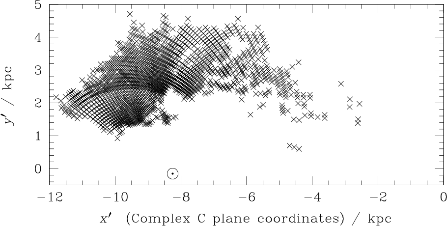
The velocity field of Complex C is given by Figure 4 of Schwarz & de Boer 2004, from which we interpolate the following two Z points: and . With the following choice for associated points to find the apparent direction vectors for each of the Z points — and — we find the normal to the supposed plane of this complex to be and a set of distances to the stream with a range of under this method, as shown in Figure 5. The stream has a significant width, across which there is some non-negligible scatter in the velocities.
It is slightly concerning that some of the clouds are rather close-by and yet they already have negative line-of-sight velocities. For example, the range of GSR velocities at ranges from -20 to, while at the range is -50 to . It is somewhat unlikely that these clouds would be able to wrap around to the other side of the Galactic centre with such infalling velocities. The near method in Section 2.1 applied to Complex C gave similar but slightly smaller distances. Both the current treatment and the near method have likely given distances which are too small to be plausible. We deduce that Complex C is not a stream lying in a plane through the Galactic Centre.
3 Correction of Radial Velocities
The method discussed in Section 2.2 was revisited, but with a correction now applied to the velocities in order to account for our offset from the Galactic centre. Whereas previously the heliocentric line-of-sight velocities corrected to the GSR were used in the energy equation, we now corrected these iteratively to actual Galactocentric radial velocities. We first calculated, using line-of-sight velocities, the zeroth order distances to the stream clouds. With the three-dimensional configuration of the stream then known to lowest order, we could transform to planar coordinates with the suppressed axis corresponding to the normal to the stream plane as defined by the three fiducial points (see Section 2.2 for definition). We discounted the third dimension — vertical offsets from the stream plane — on the basis that these deviations were small relative to both components in the plane and overall distance of the stream from the Galactic centre. We then know the approximate direction in which a particular point in the stream is moving, assuming no motion into or out of the plane. This assumption was reasonable given the size of the vertical offsets. The component of the true velocity projected along our line of sight gives the observed velocity , since radial velocities are taken to be positive if they are outwards, hence an appropriate de-projection of gives the ‘true’ velocity. This can then be re-projected along the radial vector from the Galactic centre to the stream point to give the corrected radial velocity.
We found the line-of-sight velocities to have been a slight under-estimate on the Galactocentric radial velocities for the Magellanic Stream. The maximum change in Galactocentric distance as a result of this velocity correction is approximately for the farthest point, and the smaller distances are less affected, on average by less than . We conclude that the size of the corrections, which are presented in Table 3, are small in comparison with errors that might result from the choice of method to derive the distances.
By calculating the ‘true’ velocity vector, we were also able to calculate the angular momentum vector at each point along the stream. In Figure 4, the magnitude of the -component of the angular momentum is plotted as a function of distance along the stream, where the axis is parallel to the normal to the stream plane, and nearly parallel to the Galactic axis.
In order to determine the component of velocity along the stream, we require the angle between the stream and the vector transverse to the radial vector. This can be determined from Figure 3. Since the angular momentum depends on the cotangent of this angle, the errors on the angular momenta are derived from assuming a error in this angle. Near the perigalacticon, the angle becomes close to . For such points, the associated errors become very large; these points have not been plotted. Figure 4 shows that the angular momentum along the stream is consistent with being constant within the errors.
4 Effects of the Galactic Potential
We now address the issue of the choice of potential used. Until now, we have assumed a simple logarithmic potential giving a constant circular velocity. It is instructive to check whether this is an over-simplification and we should instead be using a potential which has a power-law dependence on the Galactocentric distance. As with the radial velocity correction above, the baseline for our check is the method given in Section 2.2. The following equation results from using properties of the point in combination with a rearrangement of equation (9) with :
| (17) |
where and all other variables have the same definitions as before.
When the constant is set to a small positive quantity, a small negative correction results for the Galactocentric distances. For example, shifts the distances found with the logarithmic potential down by approximately 0.7 kpc and shifts the distances by approximately 7 kpc.
It is instructive to find the range of values of that is consistent with acceptable values of the Galaxy’s mass out to , . Imposing the total mass within this radius and a circular velocity at the Sun automatically imposes the steepness of the density profile. Since and , it follows that . If we ask, for example, that be consistent with , which is consistent with values given by Kulessa & Lynden-Bell 1992, then is restricted to values between 0.14 and . Employing a smaller mass for the Galaxy would raise the value of . If, for example, the mass range given above were applied at , then the value of corresponding would range between and . The actual range is narrower when physical demands are incorporated, such as that the Magellanic Clouds should not be at ridiculously small distances and that we should perhaps expect the circular velocity to taper off gradually between the solar position and the distance at which the farthest point on the stream resides. We would, for example, expect to be no greater than 0.1 in order that the distance to the Magellanic Clouds are not too discrepant with observationally determined values.
5 Relaxing the Angular Momentum Constraint
In previous sections, we have assumed all of the material comprising the stream to be following the same orbit, with the same value of angular momentum and energy being applicable along the entire length of the stream. We now investigate the effect of relaxing this constraint. If the material forming the Magellanic Stream had been stripped from the Clouds at the last passage through perigalacticon, the material must have undergone a change in energy and angular momentum in order for the observed streaming shape to have formed. There is an observed lag of approximately of the end of the stream relative to the position of the Magellanic Clouds.
In the course of a tidal tearing, the outer parts of the victim are torn off by the strong tides close to pericentre. For a small victim, the tidal debris will have almost the same pericentre as the remnant of the victim. Thus the energies and angular momenta of the tidal debris are related by the condition of all having the same pericentre distance. An alternative interesting way of seeing this is to imagine that near pericentre, where the tearing occurs, it is sufficient to treat the potential under which the debris moves as that of two bodies rotating about one another with angular velocity . In reality the rotation rate varies, but it will come to a maximum at pericentre so it will not be a great error to treat it as constant near there. Now an orbit in the field of two bodies rotating around one another at constant angular velocity will have a constant Jacobi integral (or energy relative to the rotating axes). The quantity will be conserved as debris leave the victim. This implies that those that gain most angular momentum from lagging just behind the victim will gain energy . This argument leads to essentially the same conclusion as the demand that the perigalactica of all the debris be the same. Hence when we deal with debris spread along the orbit, we change both energy and angular momentum in proportion and use as our parameter.
5.1 Method
We continue to use a generalised potential of the following form in the energy equation, now with an explicit constant:
| (18) |
Differentiating the potential and using the fact that the square of the circular speed at radius is given by gives the equation . Since we have both a value for the circular speed at the location of the Sun and its distance from the Galactic centre, can be calculated given a value for ; the potential at a given radius is then known. We can rearrange the energy equation by using to obtain:
| (19) |
where the prime denotes differentiation with respect to the azimuthal angle . Using equations (9), (18) and (19) for the peri- and apogalacticon gives the following equation for the angular momentum :
| (20) |
Keeping the assumption that the Clouds and stream lie in a planar configuration, the orbit of the Clouds33 3 For the purposes of this calculation, the Large and Small Magellanic Clouds — collectively referred to as ‘the Clouds’ — were taken as a combined single point at their approximate centre of mass. can be computed for a given perigalacticon and apogalacticon. The constant in the potential was set to 0.01. Note that it is not strictly necessary to have an absolute value of if we only require relative values of angular momenta.
The true current position of the Clouds was estimated to be approximately 0.7 rad from the perigalacticon that the Clouds have just passed through; we refer to this angle as the ‘offset’ angle. Note that more than half of the stream material lies on the other side of this perigalacticon. In the orbital computation, we know the time it has taken for the Clouds to cover the distance from the initial perigalacticon — where we assume the material for the stream was originally stripped — to their current position. During the same period in time, the end of the stream must have covered a smaller angle in the sky in order to have left the observable lag-angle of approximately , despite having started at the same location.
5.2 Results
We took a fixed perigalacticon distance for the Clouds and investigated the effect that changing the distance to apogalacticon has on the total change in angular momentum that occurs along the stream. For of between 80 and 180 and a fixed of 45 kpc, we find a simple relationship between and through a fit of the following form:
| (21) |
where now specifically refers to the absolute change in angular momentum from the Clouds to a point downstream. The largest difference in angular momentum arises from the least eccentric orbits. For an assumed apogalacticon of for the Magellanic Clouds, we find that , implying a 6% difference in the angular momentum between the extreme ends of the stream. For these choices of parameters, the Clouds would be positioned at and the end of the stream at . Changing only the perigalacticon to brings the Clouds slightly further in to and a slightly smaller value of . We find that the distance in an unperturbed orbit to the same azimuthal position relative to the Magellanic Clouds as the end point is only of order less than that for the perturbed orbit.
5.3 Consistency Checks
By allowing for a gradient in the angular momentum along the length of the stream, the angular position of the current perigalacticon will be different between the Clouds and the end of the stream, even though, by design, the distance of closest approach to the Galactic centre will remain the same. When setting an offset angle for the Clouds, which is taken relative to the current perigalacticon, it is important to remember that the location of perigalacticon gradually shifts along the stream. We have checked that its difference for the extreme ends of the stream is merely and hence there is little error in measuring the offset angle from the perigalacticon of the computed Magellanic Clouds’ orbit, as opposed to an averaged value.
Using the first set of parameters described in the section above, we have also checked the effect of altering the offset angle by a few percent to ensure that an error in determining this value from observational data and calculations described in Section 2.2 would not lead to a significant error in . We find that the percentage difference in this quantity resulting from a change in the offset angle is tiny, on the order of a few hundredths of a percent. An under-estimation of the offset angle by produces a greater error, on the order of a few tenths of a percent of . This is as expected, given that changes in velocity over the same angle occurs more rapidly when closer to perigalacticon than when further away. The change in angular momentum that would be required to keep the end of the stream far enough away therefore becomes slightly larger. Even for the under-estimation case, however, the errors are still relatively small.
One other point to note is that the concept of an point, defined previously as the location on the orbital stream with the highest radial velocity, is now void. This is because the stream material is not following the same orbit as that of the Clouds. A check to see whether the projected line-of-sight velocity at the tip of the stream, earlier coined the point, is consistent with the observed value at that location served as an independent test of the validity of the approach used to exploit the lag-angle in calculating the angular momentum deviation.
6 Summary and Conclusions
We have applied a variety of geometrodynamical methods to streams of high-velocity clouds in an attempt to constrain their distances. Some of these methods, including the near method, have the nice feature that distance determinations would be possible without the parameter dependency inherent in any simulations. We find, however, that the near method in particular becomes rather inaccurate when the angle subtended at the stream by becomes small. At the expense of becoming more model dependent by assuming a halo form for the Galactic potential, we have improved on this accuracy. We then find distances to the entire length of the Magellanic Stream by assuming that the gas comprising the stream nearly follows a planar orbit about the Galactic centre. We find the perigalacticon to be at and the maximum distance at the trailing end to be . The heliocentric distances are not very different from the Galactocentric distances, varying typically by or less. The centre-of-mass of the Magellanic Clouds would be at from us, according to this method; this is consistent with various observationally determined values for the Large Magellanic Cloud (see Alves 2004 for a review). Application of our methods to Complex A and C did not yield very promising results under the assumptions that were made. This indicates that our hypothesis, namely that the streams were nearly following an orbit around the Galactic centre in a well-defined plane, was not valid for these two streams of high-velocity clouds.
In this paper, we have tested the idea that streams of HVCs follow orbits. However the assumption that the orbit lies in a plane that passes through the Galactic centre is rather restrictive when applied to nearby streams that do not pass close to the Galactic Pole. It is possible to remove the restriction of a planar orbit, provided a model of the Galaxy’s potential is given. We find that the transverse velocity of the stream can be deduced from the run of radial velocities as a function of angle along the stream, provided the distance to one point of the stream is assumed. Orbits can then be computed in the given potential. Both directions in the sky and radial velocities are then computed and these are compared with the observations. Such a method and an example of its application to Complex A and the stellar Orphan stream has already been presented (Jin & Lynden-Bell 2007). We note that such methods of deriving the transverse velocity component were used in a related problem by Feitzinger et al. 1977, but probably date back to an earlier century. We are also exploring the possible existence of stream associations. Following on from these works, we hope, eventually, to give a definitive answer to the question of whether high-velocity cloud streams follow orbits around the Galaxy.
Acknowledgements
The authors thank B. Wakker and R. D. Davies for the kind use of their data for Complex A, C and the Magellanic Stream and the anonymous referee for helpful comments. SJ acknowledges financial support from PPARC.
References
- Alves (2004) Alves D. R., 2004, New Astronomy Review, 48, 659
- Belokurov et al. (2007) Belokurov V., Evans N. W., Irwin M. J., Lynden-Bell D., Yanny B., et al. 2007, ApJ, 658, 337
- Connors et al. (2006) Connors T. W., Kawata D., Gibson B. K., 2006, MNRAS, 371, 108
- Danly et al. (1993) Danly L., Albert C. E., Kuntz K. D., 1993, ApJ, 416, L29
- Feitzinger et al. (1977) Feitzinger J. V., Schmidt-Kaler T., Isserstedt J., 1977, A&A, 57, 265
- Fujimoto & Murai (1985) Fujimoto M., Murai T., 1985, in van Woerden H., Allen R. J., Burton W. B., eds, IAU Symp. 106: The Milky Way Galaxy. D. Reidel Publishing Co., Dordrecht, p. 471
- Fujimoto & Sofue (1976) Fujimoto M., Sofue Y., 1976, A&A, 47, 263
- Gardiner & Noguchi (1996) Gardiner L. T., Noguchi M., 1996, MNRAS, 278, 191
- Ibata et al. (2001) Ibata R., Irwin M., Lewis G. F., Stolte A., 2001, ApJ, 547, L133
- Jin & Lynden-Bell (2007) Jin S., Lynden-Bell D., 2007, MNRAS, 378, L64
- Kulessa & Lynden-Bell (1992) Kulessa A. S., Lynden-Bell D., 1992, MNRAS, 255, 105
- Majewski (2004) Majewski S., 2004, in Prada F., Martinez Delgado D., Mahoney T. J., eds, Satellites and Tidal Streams Vol. 327: Substructure in the Galactic Halo. Astron. Soc. Pac, p. 63
- Mastropietro et al. (2005) Mastropietro C., Moore B., Mayer L., Wadsley J., Stadel J., 2005, MNRAS, 363, 509
- Mathewson et al. (1974) Mathewson D. S., Cleary M. N., Murray J. D., 1974, ApJ, 190, 291
- Muller et al. (1963) Muller C. A., Oort J. H., Raimond E., 1963, CR Acad. Sci. Paris, 257, 1661
- Palma et al. (2003) Palma C., Majewski S. R., Siegel M. H., Patterson R. J., Ostheimer J. C., Link R., 2003, AJ, 125, 1352
- Putman et al. (2004) Putman M. E., Thom C., Gibson B. K., Staveley-Smith L., 2004, ApJ, 603, L77
- Schwarz & de Boer (2004) Schwarz U. J., de Boer K. S., 2004, in van Woerden H., Wakker B. P., Schwarz U. J., de Boer K. S., eds, ASSL Vol. 312: High Velocity Clouds. Kluwer Academic Publishers, Dordrecht, p. 55
- Sembach et al. (2002) Sembach K. R., Gibson B. K., Fenner Y., Putman M. E., 2002, ApJ, 572, 178
- Thom et al. (2006) Thom C., Putman M. E., Gibson B. K., Christlieb N., Flynn C., Beers T. C., Wilhelm R., Lee Y. S., 2006, ApJ, 638, L97
- van Woerden et al. (2000) van Woerden H., Wakker B. P., Peletier R. F., Schwarz U. J., 2000, in Kraan-Korteweg R. C., Henning P. A., Andernach H., eds, ASP Conf. Ser. 218: Mapping the Hidden Universe. pp 407
- van Woerden et al. (2004) van Woerden H., Wakker B. P., Schwarz U. J., de Boer K. S., 2004,High Velocity Clouds. Kluwer Academic Publishers, Dordrecht
- Wakker (2001) Wakker B. P., 2001, ApJS, 136, 463
Appendix A Example of the Near Method
We have tested the near method (see Section 2.1) on simulated orbits of varying orientations and distances in the logarithmic potential. The constraint on given in Section 2.1 was deduced from these test cases; one working example is shown here. The normal to the orbital plane is given by . The orbit is nearly polar but is otherwise inclined at approximately to the Galactic axis.


Figure 6 shows how the heliocentric distance to the orbit, the line-of-sight velocity and the angle change as a function of time. The orbit shown has a length of . The singular behaviour of the variables and near the point is clearly visible in Figure 7, both when using the exact orbital data and when some scatter has been applied to the direction cosines. The distance to the point, , can be calculated from the noisier plot to within a few per cent of the correct value.