Finite size corrections in the Sherrington-Kirkpatrick model
Abstract
We argue that when the number of spins in the SK model is finite, the Parisi scheme can be terminated after replica-symmetry breaking steps, where . We have checked this idea by Monte Carlo simulations: we expect the typical number of peaks and features in the (non-bond averaged) Parisi overlap function to be of order , and our counting (for samples of size up to spins) gives results which are consistent with our arguments. We can estimate the leading finite size correction for any thermodynamic quantity by finding its dependence in the Parisi scheme and then replacing by . Our predictions of how the Edwards-Anderson order parameter and the internal energy of the system approach their thermodynamic limit compare well with the results of our Monte Carlo simulations. The -dependence of the sample-to-sample fluctuations of thermodynamic quantities can also be obtained; the total internal energy should have sample-to-sample fluctuations of order , which is again consistent with the results of our numerical simulations.
pacs
75.50.Lk, 75.10.Nr, 75.40.Gb1 Introduction
The Sherrington-Kirkpatrick (SK)[1] model of spin glasses has been the subject of hundreds of papers. It is the model for which mean-field theory becomes exact in the thermodynamic limit (i.e. when , the number of spins in the model, becomes infinite). Parisi’s replica symmetry breaking (RSB) solution[2] is now known to be the correct mean-field solution[3]. Extensive studies, mostly numerical, have been made of the model at finite values. Analytically the determination of the properties of the model at finite – the finite-size corrections – is a much more challenging task in the low-temperature phase than finding the mean-field theory. At finite all the loop corrections to the mean-field solution need to be considered. Because of the massless modes present in the low-temperature phase[4] each term in the loop expansion is infinite. Hence a direct perturbative approach is impossible. A similar situation applies in finite dimensional spin glasses, already for the bulk term, when the dimension is smaller than six[5], so that one could hope at least that experience gained in studying finite size effects in the SK model might be relevant to spin glasses in physical dimensions.
Unfortunately we have been unable to find any systematic theoretical treatment of the finite-size problem. However, we have managed to obtain insights into it by examining the structure of the Parisi overlap probability distribution function (i.e. the non-averaged overlap probability distribution function) at finite values. is defined as the probability that the overlap of the spins in two copies of the system with the same realization of the quenched disorder is equal to , i.e.
| (1) |
where the Hamiltonian of the two-copy system is
| (2) |
and the sum runs over all the pairs of sites in the system. The thermal average in Eq. (1) is taken over the Boltzmann weight associated with all the possible values () of the Ising spins and . It has been known for many years that the function is very different for different realizations of the bonds. In particular it contains a very variable number of peaks, humps or shoulders. In this paper we shall systematically study the distribution of and the dependence of its average on the number of spins . We shall give numerical and analytic arguments that the mean number of features increases as , with and that , the width of the distribution of , is independent for large . The next step of our approach is to argue that the Parisi replica symmetry breaking scheme, which involves levels of symmetry breaking (where in order to achieve a stable solution has to be taken infinite in the thermodynamic limit), is stabilized at finite at a value by self-energy contributions (whose dependence is estimated in Appendix A). As a consequence we can estimate for a given system size and because (see Sec. 8), we can understand the size dependence of the number of peaks/features in .
The next step towards predicting the exponents which give the leading dependence of the corrections to the thermodynamic limit of quantities such as the internal energy per spin is simply to use the RSB scheme to compute the dependence of the quantity on . For example , where denotes the value of the internal energy in the infinite limit[6]. Our prescription for evaluating the exponents of the leading finite size corrections is to set ; this implies that the leading finite size correction to the thermodynamic limit of the internal energy per spin should be of order . Since arguments of this type do not have the strength of a theorem and can only be suggestive of the possible behaviour, we have checked our arguments with extensive Monte Carlo simulations. We have computed many quantities at a number of different values of the temperature. Our results for the internal energy are reported in Sec. 5. That data strongly supports the value of predicted by our approach for the exponent of the leading finite-size correction.
Similarly, the Edwards-Anderson order parameter at finite differs from its infinite form by a term of order . Hence we predict that the finite size shift of should be of , and we present numerical evidence for this behaviour in Sec. 6.
Our approach can be used to investigate the sample-to-sample fluctuations of any quantity by relating them to the sample-to-sample variation in the number of features in , . For the internal energy we shall find in Sec. 7 numerical evidence consistent with this approach, together with a discussion of the behaviour of the sample-to-sample fluctuations in the critical regime and in the high-temperature phase. Our basic prediction is that the sample-to-sample fluctuations in the total free energy of a system of spins are of order where the exponent . There have been numerous attempts to determine this exponent, both numerically and analytically, and we review them also in Sec.7.
Because the peaks/features in are caused by the overlap of pure states, in particular those states whose free energies are of order from that of the lowest free energy state, one can relate the number of these pure states to the number of peaks using the relation . This connection is simplified because of the ultrametric organization of states in the SK model and the details of the argument are given in Sec. 8. In Sec. 9 we discuss the relation of these ideas with the behaviour of finite dimensional spin glasses.
2 Theoretical framework
Our Monte Carlo studies of the Parisi overlap probability distribution function for systems of spins (with up to ) show that the number of peaks/features is usually quite small, and that it increases only slowly with , apparently as , with . Our approach to the study of finite size effects in the SK model is to argue that , the average number of such peaks/features for a system of size , can be connected to a truncation of Parisi’s RSB scheme at its th step, with .
The Parisi scheme at the -th level of RSB parametrizes the bond-average of , , by a series of delta functions at various values of , viz ;
| (3) |
The weights of the delta functions and their positions are the variational parameters that one optimizes to obtain the Parisi solution. In the thermodynamic limit, where goes to infinity, a Parisi RSB solution with is only stable if is taken to infinity. We argue that in finite size systems the self-energy corrections to the Parisi solution can stabilize an RSB solution with a finite value of , and we will argue that . (In zero field so the number of peaks/features . However, if just happens to be zero, i.e. there is a peak at the origin, then ).
Consider the single-valley replicon correlation function . At wavevector its Fourier transform takes the form described in Ref. [4], and at Gaussian order, , both for and . (Strictly speaking in the SK model the only possible value which can take is zero, but we will find it useful to consider non-zero values of ). Right at , is infinite in the thermodynamic limit. For finite , the self-energy corrections neglected at Gaussian order will be shown in Appendix A to produce a divergence growing as . Schematically
| (4) |
so that the self-energy is of order .
Now for finite values of in the Parisi RSB scheme, the Gaussian propagator is unstable and behaves as[6]
| (5) |
in the regime near the transition temperature where is small. The instability at only disappears when one takes the infinite limit. Our basic idea is that for finite this instability can be removed by the stabilizing effect of the self-energy . Then if stability will be achieved when
| (6) |
In other words, when , there will be no need to break the symmetry further (at least to achieve stability). This would explain why the number of peaks/features in increases as (see Fig. 1).
Our procedure to determine the finite size corrections to scaling of any thermodynamic quantity proceeds in a similar fashion. First one obtains from RSB calculations the approximation for the quantity. Thus the free energy per spin below but near is to order , and at large values of [6]
| (7) |
To estimate the dependence of the finite size corrections we replace by . This gives a term in which scales as , which is in excellent agreement with numerical studies[7]. Just as the self-energy corrections to Eq. (5) change the sign of , we would expect that the higher loop corrections to the free energy will also change the sign of this correction, but not its dependence.
A similar argument can be given for other quantities. The additional terms in the internal energy per spin below at order in the RSB procedure are[6]
| (8) |
Substituting as before for , the finite size corrections to the internal energy would be expected to be of order .
The Edwards-Anderson order parameter[6] is to order
| (9) |
correct to order . It is thus to be expected on substituting for that the finite size corrections to are of order . If one defines for finite-size systems as the value of at which the Parisi overlap function peaks, then such an dependence is in excellent agreement with both existing numerical and theoretical arguments[8]. We postpone to Section 6 the comparison with the results of our numerical analysis of the scaling behaviour of .
Our approach can be extended to determine the dependence of sample-to-sample fluctuations of, say, the internal energy or the free energy. In Ref. [9] it was shown that the variance of the sample-to-sample fluctuations of the extensive free energy varies as a quantity , which at Gaussian order has the property . At finite RSB of order , an exact expression for this quantity was given in Ref. [10]. As shown in Appendix B, it can be evaluated when (which is originally a wave vector) is replaced by the self-energy. One gets that
| (10) |
where is some known function (see Appendix B). This shows that the variance of is of order , with typical fluctuations being of order .
From this result one can compute the sample-to-sample fluctuations of . To do this we shall suppose that the sample-to-sample fluctuation of is of order . Then Eq. (7) implies that the sample-to-sample fluctuation of the extensive free energy behaves as
| (11) |
Given that , it follows that is of , that is, independent of .
We have determined the sample-to-sample fluctuations of the internal energy in the course of our simulations, and their dependence can be predicted by extension of these arguments. From Eq. (8), the sample-to-sample variation of the full internal energy is
| (12) |
Substituting for and , it follows that . These sample-to-sample fluctuations appear to diverge at , but Eq. 12 only holds in the RSB region, which is outside the critical regime, (which is defined by the limits , , with fixed [11]).
All these arguments are intuitive rather than rigorous. As a consequence we have attempted to check them by numerical simulations of the finite size SK model.
3 The Monte Carlo simulation
We have based our analysis on a large set of numerical data produced by the large scale parallel tempering simulation of Ref. [12] and [13], supplemented by a new large scale simulation for lattices with spins.
The quenched random couplings of our system can take the two values with equal probability; the use of such binary couplings allows to write computer codes that run much faster than, say, when using quenched random couplings assigned under a Gaussian distribution. We assume that the interesting leading scaling behaviour is the same, for example, when using binary or Gaussian couplings.
We report in Table 1 the relevant parameters of our numerical simulations. The temperatures allowed to the parallel tempering steps are in the range .
| 64 | 1000 K | 400 K | 1024 |
| 128 | 1000 K | 400 K | 8192 |
| 256 | 1000 K | 400 K | 1024 |
| 512 | 200 K | 200 K | 1024 |
| 1024 | 1000 K | 400 K | 1024 |
| 2048 | 200 K | 200 K | 512 |
| 4096 | 500 K | 400 K | 256 |
A parallel tempering sweep consists of one Metropolis sweep (all spins are updated in lexicographic order) followed by a temperature exchange sweep (we try to exchange adjacent values of in sequential order). The balance between the number of sweeps performed for each disorder sample and the number of disorder samples included has been chosen cautiously in order to avoid any possible bias due to a non-perfect thermalization; we have chosen a safe compromise favouring, at fixed amount of computer time, the number of sweeps over the number of disorder samples. We have checked the quality of thermalization by monitoring for example the value of as a function of the Monte Carlo time, starting from an ordered initial spin configurations (all spins equal to one). For all values of and the disorder averaged data do not drift appreciably already after a couple of thousands sweeps, i.e. far before we start taking measurements. A second important test is provided by the symmetry of the individual ’s that is very good for most samples (See Sect. 4).
In the rest of this note we will denote by the average over the quenched disorder, the total internal energy and and its standard deviation, with .
4 The structure of
As mentioned before, the function is very different for different realizations of the bonds. Fig. 2 shows eight such distributions for the lowest temperature value () of the largest system () we have simulated. The symmetry of the plots under inversion of the overlap is excellent: one can see that even very small peaks appear with their reflected counterpart, and this is a remarkable check of good thermalization. The only mild asymmetries one can see concern the peaks heights, connected to the population of the different “pure states to be”, that is a very difficult quantity to estimate by Monte Carlo integration (just think about the two peaks in the magnetization distribution for the usual Ising model in three dimension below the Curie temperature). Each of the exhibits a given number of features (well formed peaks, humps, shoulders on the side of a peak, and so on) that we are interested to determine in order to compute its disorder expectation value and the scaling behavior of with .


Peaks/feature counting is not at all a trivial issue when dealing with noisy data. The first assumption must be that the statistical accuracy of the data set is good enough not to hide important features (in this respect it is possible that further improvements to the Monte Carlo scheme could help: one could check for example if using multi-overlap algorithms[14, 15] could be of help). Under this assumption we have developed a computer code that counts the number of peaks. The first step is based on smoothing up the (symmetrized) data for . The second step determines the peaks of the soothed data: the peaks are defined as local maxima of where a valley at least lower than a percentage of the peak height follows the peak on both sides (we have selected and we have relaxed the depth condition for valleys that include one of the two frontiers of the support, i.e. ). As a third and last step we impose a cutoff on the putative peak heights: we discard any peak of height lower than of the highest peak present in the for the given disorder sample. In what follows, we will call “automatic peak counting” this procedure to determine features.
We did not push the coding to include in our automatic peak counting the more complex structures which visual inspection spots: an automatic approach to such a complex task needs great care to avoid arbitrary choices that could lead to misleading conclusions.
For example it looks clear that the first plot of Fig. 2 (the upper left figure) is characterized by four features, two for and the two symmetric ones for . The first feature is the clear peak that also the computer code finds, while the second very clear feature is the shoulder on the peak: this shoulder is naturally interpreted as a second unresolved peak, too wide to be an isolated feature, but whose presence is very clear to the observer. In other words it is clear that a correct analysis of this feature would lead to and that the conclusion reached by our computer code is not careful enough (as an optimistic remark let us add that it is possible that the lazy procedure could lead asymptotically to the same scaling behaviour of a more careful counting). To be on the safe side, we have carried out the tedious task of looking at the first ’s for and estimating by eye the number of features for every graph. This procedure will be called “visual inspection” in what follows.
We show the behaviour of as a function of for in Fig. 1 for the visual inspection and in Fig. 3 for the automatic peak counting. The statistical errors are estimated from the fluctuations between the disorder samples. Our visual inspection gives on average between one and two extra features that are not found by the automatic computer counting. The best fits to the form for the two cases give the exponents for the visual inspection and for the automatic count. The difference between the estimated error bars mainly reflects the number of disorder samples considered in the two cases. Our prediction is . Our result for is on the top of it but it has a huge statistical error, while our result for is not consistent with at more than two standard deviations (but is of uncertain relevance). It is important to notice that here we are dealing with a quantity that grows very slowly and is very small even for our largest systems, and that pre-asymptotic effects could be large.
In Fig. 4 we show
| (13) |
i.e. the fluctuations of (as determined by visual inspection), together with the best fit to the form . The best fit is obtained for : our theoretical estimate in Sec. 2 of the value of the exponent was zero; our numerical work is consistent with this estimate, although greater precision is really needed before the result can be regarded as definitive.
In Fig. 5 we give the empirical distribution of the number of features obtained by visual inspection for and : the distribution is very wide. It is also clear from the figure that even values of are more common than odd values: this is expected, since odd values are only obtained in cases where has a peak in .

5 Finite size shift in the energy
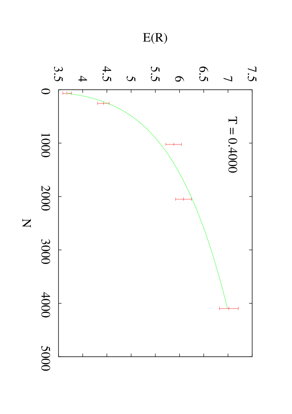
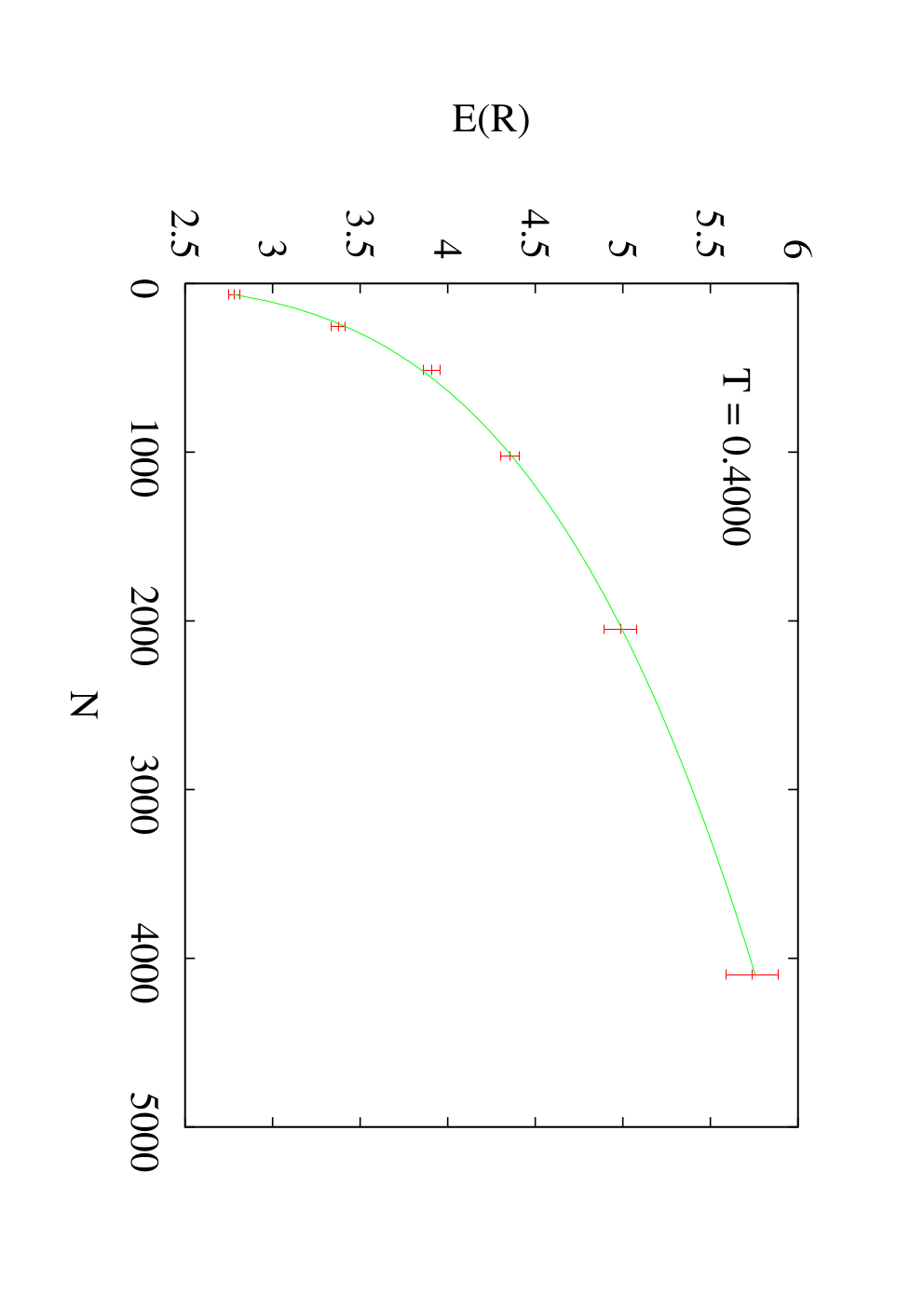
In Fig. 6 we show the internal energy per spin as a function of for our lowest temperature (that we believe is low enough to be free of effects from the critical point). The statistical errors are again estimated from the fluctuations between the disorder samples.

In the same figure we show a fit to the form , using the value from Ref. [16]. The best fit is obtained for , with a of for degrees of freedom. The presence of slow decaying sub-leading corrections (the dominant sub-leading contribution behaves like , barely faster than ) explains presumably why the is larger than the number of degrees of freedom. The importance of the corrections to the leading behavior (together with some statistical oddness) shows up in Fig. 7, where we plot as a function of : this is a way to focus on the deviations from the leading behaviour. We do believe that the three leftmost odd looking data points in Fig. 7 are due to a statistical fluctuation. The curve is a fit to , which is the form we would expect from a correction to the internal energy per spin. Based on Figs. 6, 7 and similar plots at different temperature values, we conclude that our numerical data are consistent with an exponent in the whole spin glass phase. We disagree with the conclusions of Ref. [17] that are based on data with , namely a region that is discarded altogether in our fits (see Ref. [18] for a detailed comparison).

6 The Edwards-Anderson order parameter
We have studied the finite size behaviour of the Edwards–Anderson order parameter , improving the analysis of Ref. [8]. We define on a finite system as the location of the maximum of the disorder averaged . The exact procedure is the following: we first symmetrize our data for , then we determine the maximum value reached by the function (we call it ) and finally we compute by means of a quadratic fit of the data in the range of positive values such that , using the same weights for all data points. This gives us an estimate of that is not forced to take discrete values: statistical errors are obtained through a jackknife analysis (obviously a jackknife approach would not make sense if was constrained to take discrete values).
We have compared the values we have obtained for to values obtained with shorter numerical simulations, and there is an excellent agreement: this strongly suggests that the procedure we have used to determine has no appreciable statistical bias. We show in Fig. 8 our data for as a function of for , together with our best fit (using data with ) that uses the infinite volume result from Ref. [16]. The value of is for degrees of freedom, suggesting that in this case sub-leading corrections are not very relevant. The small data exhibit larger corrections from the asymptotic behaviour than the ones for the internal energy. This is not unexpected since the definition of on a finite system is involved: for example the intrinsic resolution of the determination of in a finite system is (that is close to for ), a value that is exactly on the scale of the deviations that we observe.

7 The sample-to-sample fluctuations of the internal energy
We have also analyzed the fluctuations of the internal energy between different bond realizations using as a measure
| (14) |
The issue of the scaling behaviour of the free energy fluctuations in the SK model has been investigated intensively over the years. Let us define an exponent by the equation
| (15) |
Our theoretical approach suggests that should be . The first investigation we know of is the numerical work of Ref. [19] at which gave (on very small samples) the result , compatible with . The later theoretical analysis of Ref. [20] gives . However, there is a caveat to this conclusion. What is effectively calculated is the tail of the probability distribution of the free energy on the low-free energy side [21]; in order to get and one has to assume that the dependence of the fluctuations in the tail equals the one of the standard deviation of the free energy. Ultimately these analyses relate the value of to the order of the first non-linear term in the expansion of the replicated free energy in powers of (the number of replicas), which is the term [4]. More recently, several authors, using exact or heuristic ground states determination algorithms, have found zero temperature values compatible[22, 23, 24, 25, 26, 27] with , some excluding[22, 23, 25, 26] the value, some not[24, 27]. Analytical arguments in support of the value can be found in Refs. [28, 24]. Finally a recent numerical simulation[29] using an innovative method obtains in the low phase. Clearly, the situation is far from being settled. It should be clear that in the numerical approach it is extremely hard to distinguish with confidence exponents as close as and when the range of variations of is small (typically one decade), the more so as the functional form of the next correction is unknown. A further difficulty is that exact algorithms are limited to very small systems and heuristic algorithms are heuristic.
The above results are for the free energy. The problem for the internal energy at finite temperature has never, to our knowledge, been studied numerically; we will consider here finite, low temperature values, and this will allow us to analyze both the low phase and the limit.
Let be the energy measured at some temperature during the numerical simulation of a system with a given realization of the disorder (this is what we call a sample of our system). comes from the average of values, and we can use the quantity
| (16) |
where is the number of samples, to estimate
| (17) |
At leading order and are related through
| (18) |
where is the integrated autocorrelation time for the energy at temperature , is the specific heat and is the number of parallel tempering sweeps performed during the measurement phase of the simulation (we measure the energy after every Metropolis sweep of the system).
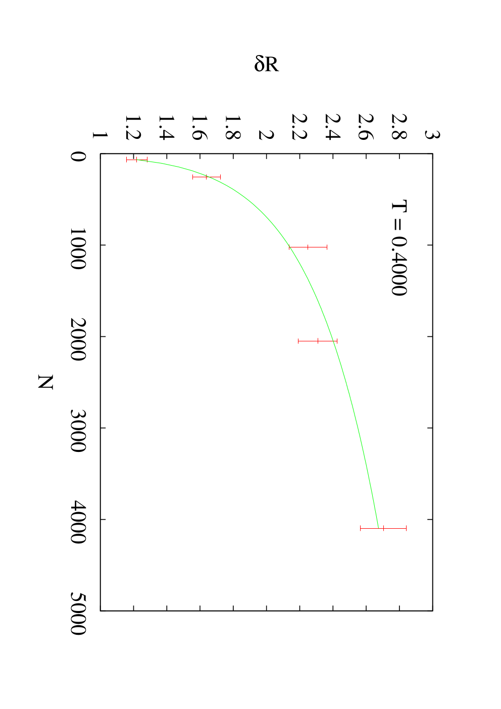
It turns out that in our numerical data the second term in Eq. 18 is negligible, as we have checked by comparing the estimates of in different numerical simulations for the same set of disorder couplings (with and ) using the first parallel tempering (PT) sweeps and the second PT sweeps after thermalization. To the best of our knowledge the autocorrelation time of the parallel tempering algorithm has never been measured for the SK model, and our results show that it is very small. Our results for as a function of can be found in Fig. 9.

Fig. 10 shows the scaling behaviour of for our lowest temperature. The leading exponent is compatible with the value but our statistical (and systematic) accuracy is not good enough to allow us to rule out the value : the main culprits are the data points for large systems (mostly and ), and we would need a much larger number of samples to have a precise determination of this exponent from Fig. 10 only.

In the critical region , where are the sample to sample fluctuations of the total free energy[20] and . The sample to sample internal energy fluctuations are related to the derivative of and they scale as , where goes like at large negative , see Fig. 11, and is a constant at , i.e. . The scaling is excellent in the paramagnetic phase (on the left) and in the spin glass phase where is small, namely before the -RSB effects start to be important, leading to a different behaviour. Fig. 11 shows clearly the two scaling regimes. The -RSB effects are only present for , in the regime where is large [30] so multiple pure states can exist. In the finite-size critical regime one has fixed with going to zero. This makes go to zero, so that in the critical regime RSB effects are absent.

In Fig. 12, we visualize the scaling behaviour of in a different way; we show the exponent obtained from a fit of to the form as a function of . This plot is consistent with the guess that the exponent at takes a value of : in order to get a value of we should have a very complex dependence of the effective exponent. The situation at and exactly at is more complicated: it is possible to see that finite size effects bring down the value of the exponent with increasing lattice size, and a scenario where the exponent is for all (but with large finite size corrections) is plausible and consistent with the data.

8 The number of pure states
It is useful to consider how the peaks in arise. Suppose we have just two states, state and its spin reverse . Then using the definition of in Eq. 1, if copy is in and copy is also in there will be a peak at at . If both copies are in , there will also be a peak at . However, if copy is in state and copy is in state , that will produce a peak at : the same will be true when copy is in state and copy is in state .
Suppose now we have states, , , , . Because (in the infinite volume limit) is the same for all states the overlaps , , , are all , and , , , are all . The overlaps ==, and =-=, giving 4 peaks in total. (If we have peaks only). However, the peak at will not in general have the same weight as that at .
Then, from the above, states give peaks and states give peaks (if all involved overlaps are large than zero).
With three states , and the effects of the ultrametric organization of states start to play a role. Besides the peak at , there could be overlaps , and making at most peaks (if all the overlaps are nonzero.). But ultrametricity says that either all three q’s are equal or are equal, making at most peaks ( peaks when one includes the time-reversed states).
With four states , , and , besides the peak at , there are the overlaps , , , , , , but here ultrametricity limits one to distinct possibilities, making peaks in total (and when one includes the time-reversed states).
There is clearly a pattern here; if states are organized ultrametrically their number is equal to the number of peaks of (plus one if there is a peak at ). We are thus predicting that the number of pure states grows with as . These pure states are those whose total free energy is of order from that of the lowest free energy state. It is only the overlaps of these low-lying states which can produce detectable features in .
Another way of determining the number of pure states at level is to observe that if one starts from the bottom (the leaves) of a genealogical tree, and moves towards the ancestors, points that are going up can only meet at the bifurcations of the tree. Hence the number of overlaps is equal to the number of levels in the tree.
9 Application to a finite number of dimensions
The exponent which determines the sample-to-sample fluctuations of the free energy of the SK model has a significance beyond this model as it appears in the theory of the interface free energy of finite dimensional spin glasses.
In Ref. [28] it was shown by going to one-loop order about the Parisi RSB mean-field solution that the variance of the interface free energy associated with the change in the free energy on going from periodic to antiperiodic boundary conditions, , is of the form
| (19) |
Here the system is of length in the direction, and it is periodic and of length in the transverse dimensions. The change from periodic to anti-periodic boundary conditions is done by flipping the sign of the bonds in a hyperplane perpendicular to the -axis. It follows that . is the bond-averaged variance of the free energy of the SK model containing spins. Eq. (19) is valid at least to one loop order, and its form is probably unchanged whenever the loop expansion is possible; the loop expansion is well-defined in the low-temperature spin glass state when , but its existence is problematic for (see Ref. [4]).
The first term in Eq. (19) is of the standard aspect-ratio scaling form [31, 32], where the zero-temperature scaling exponent is equal to . When is of order , is of order , i.e. of order if . This term is not of the standard aspect-ratio scaling form; it depends instead on the total number of spins in the system. This reflects the fact that in RSB situations domain walls have a fractal dimension equal to , i.e. they are space filling. For example in dimension , where we know that we do not have a broken symmetry phase, domain walls are fractal with . The variance of the interface free energy is dominated by the SK like term for all provided that . If , one would expect that numerical studies of the defect energy in six dimensions would suggest a value of close to unity; exactly in Boettcher[25] found that . It is possible that when the standard aspect-ratio scaling form will dominate. (Of course, when , the one-loop expression for the interface free energy will no longer be adequate). Thus the dominant term in the dependence of the interface free energy could have very different forms above and below six dimensions; note that plays a special role only if the exponent is exactly .
For the loop expansion about the Parisi RSB state becomes problematical but it is clearly possible that the essential features of RSB might survive even in , and that the appropriate analytic approach could allow to make that clear. Another possibility is that for the droplet picture of spin glasses [33, 34] would apply instead, as advocated in Ref. [5], so that the nature of the spin glass state would change from being RSB like for to being replica symmetric for . According to this picture should become just two delta functions at in the thermodynamic limit, corresponding to just a state and its time reverse. (In fact, for finite systems in three dimensions, appears strikingly similar to that of the finite SK model[35]. Unfortunately no systematic study has been made as to how the number of peaks, humps and shoulders evolves with system size; such an investigation could be very informative as regards the true nature of the three-dimensional spin glass state.)
We have argued here that for the finite SK model the replica symmetry breaking is stabilized at a finite value of by self-energy effects. The replica symmetric state of the droplet picture corresponds to having . Thus were the droplet picture to be the valid description of spin glasses below six dimensions (and some of the authors of this paper would argue that this is unlikely!), the same mechanism could stabilize the replica symmetric state. While perturbatively there seems to be no way that the replica symmetric state could be stable, it is possible that if the full self-energy corrections about that state could be included into the calculation, then replica symmetry might be maintained [5].
Acknowledgments
We thank Giorgio Parisi for interesting verbal and virtual conversations about many of the topics discussed in this note. We thank Marc Mézard for useful comments and advice, and Jean-Philippe Bouchaud for discussions. We also thank Andrea Crisanti and Tommaso Rizzo for allowing us to analyze their numerical data.
Appendix A The dependence of the self-energy
In this Appendix we shall estimate the dependence of the self-energy . This is needed for our argument that the number of features scale as . A direct calculation of would be impractical: it would involve summing diagrams to all orders. Because of that we will obtain the dependence of indirectly via a study of the TAP equations [36] of the model.
The TAP equations provide a non-replica way of finding single-valley correlations. For the magnetization at site within a single state they give
| (20) |
The spin glass susceptibility is defined as
| (21) |
When the right-hand side is bond-averaged over the exchange interactions we obtain . In the following we will only consider the case of zero magnetic field, .
It is convenient to express in terms of the eigenvalues of the Hessian matrix of the second derivatives of the TAP free energy[37]:
| (22) | |||||
In terms of the eigenvalues of ,
| (23) |
which in terms of the density of states becomes
| (24) |
The first term on the right hand side of Eq. (22) is of order and is smaller than the other terms which are either of order , or on the diagonal, of order 1. It will be dropped. (We are focusing in this work on the low-lying TAP states – the pure states – where the mechanism for splitting off an isolated eigenvalue as in Ref. [38] cannot operate.) A stable solution of the TAP equations which corresponds to a minimum requires all the eigenvalues of the matrix to be positive. For pure states, is non-zero right to the origin; at small (see Ref. [37]) one has that
| (25) |
With this form for , the integral in Eq. (24) would be divergent without its lower cutoff at . The dependence of itself can be estimated by setting
| (26) |
which means that . Using this result, we can estimate the dependence of as using Eq. (24). Notice that this result would also apply at .
In fact there is a very simple direct argument for the behaviour at . According to Refs. [11, 5] for ,
| (27) |
so that as goes to zero, that is, at , .
We would not expect that bond-averaging to get will modify this dependence since single-valley quantities are expected to be self-averaging.
Thus for , the single valley spin glass susceptibility diverges as . This implies that the typical value of , the order of replica symmetry breaking in a finite system of spins, will be via Eq. (6) of order . The data in Fig. 1 is clearly consistent with this expectation.


We have tested numerically the prediction using the iteration procedure described in Ref. [39]. This method allows us to find many TAP states even for large system sizes (see Ref. [39] for a discussion of the proximity of the iteration algorithm to a dynamical critical point and the influence of this on the free energy of the states found – here we chose the proximity for each system size in such a way that we get the same free energy range for all system sizes). Using systems with , , , , and at a temperature of , we have calculated the Hessian for every state found. The diagonalization of the Hessians was done using arbitrary precision arithmetic (with an accuracy of decimal digits) since these matrices are extremely ill-conditioned and so they are hard to diagonalize: standard packages, for instance the LAPACK routines, fail at the task. The eigenvalues were used to calculate as in Eq. (23). The results are shown in Fig. 13.
Surprisingly, appears to grow faster than . We believe, however, that this is a finite size effect. To back up this claim, we show in Fig. 14 a scaling plot of the averaged integrated eigenvalue density of the Hessians of sizes and .
The expectation is that in the thermodynamic limit this function goes as for small (corresponding to ). For finite there is a cutoff around . The natural expectation is that this cutoff is of the form with a scaling function . This is verified in Fig. 14. The arguments sketched above which lead to the prediction for large can only be expected to be valid when the interval in which prevails is large enough. This interval can be identified as the horizontal (or nearly horizontal) stretch in Fig. 14. Clearly, this interval is very small as it is not even one decade for the available system sizes. The conclusion is, therefore, that we cannot yet expect to see the asymptotic scaling behaviour. It is not possible to go to larger system sizes as the arbitrary precision diagonalization of the Hessians becomes computationally too expensive.
Appendix B Free energy fluctuations and
According to Ref. [10], the exact expression for the quantity for a finite number of replica symmetry breaking steps and for the truncated model with Hamiltonian
| (28) |
is
| (29) |
where
| (33) | |||||
| (34) |
and is the solution of
| (35) |
When the expressions for and are inserted, Eq. (29) can be rewritten as
| (36) | |||||
We are interested in the behaviour for small where diverges as approaches . It is easy to see that the first two terms of the former expression are well behaved in this limit. The divergence in must therefore come from the last term, which will be denoted by . Defining
| (37) |
and renumbering the sums to start from it can be cast in the form
| (38) | |||||
While was a finite-dimensional wave vector in Ref. [10], here we consider it as a proxy for the self-energy as we are dealing with the SK model. Substituting for and making the usual replacement (where the constant is large enough to guarantee stability) yields (to leading order in ) and . The function is defined by the remaining prefactors and the sums (with upper bounds set to infinity) in Eq. (38). This shows that the typical sample-to-sample fluctuations of the free energy are of order .
References
- [1] D. Sherrington, and S. Kirkpatrick, Phys. Rev. Lett 35 1792 (1975).
- [2] G. Parisi, J. Phys. A 13 L115 (1980).
- [3] M. Talagrand, Spin Glasses: a challenge for mathematicians. Mean field theory and cavity method (Springer Verlag, Berlin 2003).
- [4] C. De Dominicis, I. Kondor and T. Temesvári, in Spin glasses and random fields, edited by A. P. Young (World Scientific, London 1997). See also ArXiV:cond-mat/9705215v1.
- [5] M. A. Moore, J. Phys. A 38, L783 (2005).
- [6] V. Janis̆ and A. Klíc̆, Phys. Rev. B 74, 054410 (2006).
- [7] A. Billoire, Phys. Rev. B 73, 132201 (2006).
- [8] A. Billoire, S. Franz and E. Marinari, J. Phys. A 36, 15 (2003).
- [9] T. Aspelmeier and M. A. Moore, Phys. Rev. Lett. 90, 177201 (2003).
- [10] C. De Dominicis and P. Di Francesco, J. Phys. A 36, 10955 (2003).
- [11] J. Yeo, M. A. Moore and T. Aspelmeier, J. Phys. A 38, 4027 (2005).
- [12] A. Billoire and E. Marinari, J. Phys. A 33, L265 (2000).
- [13] A. Billoire and E. Marinari: Europhys. Lett. 60, 775 (2002).
- [14] B. A. Berg and W. Janke, Phys. Rev. Lett. 80, 4771 (1998).
- [15] B. A. Berg, A. Billoire and W. Janke, Phys. Rev. B 61, 12143 (2000).
- [16] A. Crisanti and T. Rizzo, Phys. Rev. E 65, 046137 (2002), and private communication.
- [17] H. G. Katzgraber, and I. A. Campbell, Phys. Rev. B 68, 180402(R) (2003).
- [18] A. Billoire, in Rugged Free Energy Landscape, Springer Lecture Notes in Physics, edited by W. Janke (Springer, Berlin-Heidelberg 2007).
- [19] S. Cabasino, E. Marinari, P. Paolucci and G.Parisi, J. Phys. A. Math Gen 21 (1988) 4201.
- [20] A. Crisanti, G. Paladin, H.-J. Sommers and A. Vulpiani, J. Phys. I France 2 (1992) 1325.
- [21] G. Parisi and T. Rizzo, cond-mat/0706.1180.
- [22] M. Palassini, PhD thesis, Scuola Normale Superiore di Pisa, 2000, unpublished.
- [23] M. Palassini, preprint ArXiV:cond-mat/0307713.
- [24] J.-P. Bouchaud, F. Krzakala, and O. Martin, Phys. Rev. B 68, 224404 (2003).
- [25] S. Böttcher, Eur. Phys. J. B 31, 29 (2003); ibid. 46, 501 (2005).
- [26] H. G. Katzgraber, M. Körner, F. Liers, M. Jünger and A. K. Hartmann, Phys. Rev. B 72, 094421 (2005).
- [27] K. Pál, Physica A 367, 261 (2006).
- [28] T. Aspelmeier, M. A. Moore and A. P. Young, Phys. Rev. Lett. 90, 127202 (2003).
- [29] M. Goethe and T. Aspelmeier, preprint ArXiV:cond-mat/0610228.
- [30] A. J. Bray and M. A. Moore, J. Phys. C 13, L469 (1980).
- [31] A. C. Carter, A. J. Bray, and M. A. Moore, Phys. Rev. Lett. 88, 0277201 (2002).
- [32] A. K. Hartmann, A. J. Bray, A. C. Carter, M. A.Moore, and A. P. Young, Phys. Rev. B 66, 224401 (2002).
- [33] A. J. Bray and M. A. Moore, Lecture Notes in Physics 275, 121 (1987).
- [34] D. S. Fisher and D. A. Huse, Phys. Rev. B 38, 386 (1988).
- [35] G. Parisi, preprint ArXiV:0706.0094v1.
- [36] D. J. Thouless, P. W. Anderson and R. G. Palmer, Phil. Mag. 35 593 (1977).
- [37] A. J. Bray and M. A. Moore, J. Phys. C 12, L441 (1979).
- [38] T. Aspelmeier, A. J. Bray and M. A. Moore, Phys. Rev. Lett. 92, 087203 (2004).
- [39] T. Aspelmeier, R. Blythe, A. J. Bray and M. A. Moore, Phys. Rev. B 74, 184411 (2006).