Replica-symmetry breaking: discrete and continuous schemes in the Sherrington-Kirkpatrick modelJournal: JPA

A hierarchical character of the phase space of the SK model is expressed in a hierarchy of order parameters standing for generations of the replicated spins. Each generation is characterised by a pair of numbers $m_{l}$ and $\chi_{l}$. The former ”geometric” parameter expresses a probability with which the original spins are affected by spins from the replicated systems and the latter represents the strength with which the original and the replicated spins from the $l$th hierarchy interact [7]. A phase space with $K$ hierarchies ($K$RSB) is characterised in addition to the SK order parameter $q$ also by $K$ pairs $\{m_{l},\chi_{l}\}$ with $l=1,\ldots,K$.¹¹ 1 We use here, in accordance with Ref. [7], a decreasing sequence of overlap susceptibilities $\chi_{l}$ instead of parameters $q_{l}$ in the Parisi notation. The two sequences are simply related $\chi_{l}=q_{K+1-l}-q_{0}$ for $l=1,\ldots,K+1$ . All these parameters are determined from stationarity equations for a hierarchical free energy with $K$ hierarchies.

It is not the set of pairs $\{m_{l},\chi_{l}\}$ that explicitly appears in the hierarchical free energy. In fact, we can construct a free energy functional for either $\chi_{l},\Delta m_{l}=m_{l-1}-m_{l}$ or $m_{l},\Delta\chi_{l}=\chi_{l}-\chi_{l+1}$ for $l=1,\ldots,K$ with boundary conditions $m_{0}=1$ and $\chi_{K+1}=0$. Both set of parameters $m_{l}$ and $\chi_{l}$ form a decreasing sequence. The general formula for the hierarchical free energy with the former pairs was introduced in Ref. [8] while the latter in Ref. [7] that we use also in this paper.

The free energy with $K$ hierarchies is characterised by $2K+1$ order parameters. It is the SK order parameter $q$ and $K$ pairs $\{m_{l},\Delta\chi_{l}\}$, $l=1,\ldots,K$. The averaged free-energy density with these order parameters reads

A hierarchical structure of this free energy is evident from the way its interacting part $\ln\mathcal{Z}_{K}$ is constructed. It is the final state in a sequence of partition functions defined inductively

with the initial condition $\mathcal{Z}_{0}=\cosh\left[\beta\left(h+\eta\sqrt{q}+\sum_{l=1}^{K}\lambda_{l}\sqrt{\Delta\chi_{l}}\right)\right]$. We abbreviated the Gaussian differential $\mathcal{D}\lambda\equiv d\lambda\exp\{-\lambda^{2}/2\}/\sqrt{2\pi}$.

Free energy (2.1) is a generalisation of 1RSB and 2RSB solutions obtained by Parisi. It is a generating functional for all physical quantities of a $K$-level hierarchical solution. The physical values of the order parameters $q,\Delta\chi_{1},m_{1},\ldots,\Delta\chi_{K},m_{K}$ are determined from stationarity equations maximising free energy $f^{K}$. To represent the corresponding stationarity equations we introduce a set of hierarchical density matrices in the space of fluctuating random fields $\lambda_{l}$. We define $\rho_{l}(\eta,\lambda_{K},\ldots,\lambda_{l})=\mathcal{Z}_{l}^{m_{l}}/\left\langle\mathcal{Z}_{l}^{m_{l}}\right\rangle_{\lambda_{l}}$ where $\langle X(\lambda_{l})\rangle_{\lambda_{l}}=\int_{-\infty}^{\infty}\mathcal{D}\lambda_{l}\ X(\lambda_{l})$. We further introduce short-hand notations $t\equiv\tanh\left[\beta\left(h+\eta\sqrt{q}+\sum_{l=1}^{K}\lambda_{l}\sqrt{\Delta\chi_{l}}\right)\right]$ and $\langle t\rangle_{l}(\eta;\lambda_{K},\ldots,\lambda_{l+1})=\langle\rho_{l}\ldots\langle\rho_{1}t\rangle_{\lambda_{1}}\ldots\rangle_{\lambda_{l}}$.

It is now a straightforward task to derive equations for the order parameters from the saddle-point equations of functional $f^{K}$. We obtain

where index $l=1,\ldots,K$.

The discrete RSB scheme does not determine a single solution of the original spin model, but rather a set of solutions labelled by the number of hierarchies explicitly taken into account. Parameter $K$ is hence a free index that is not determined from the free energy. Its physical value is fixed by thermodynamic stability. We take so many hierarchies of replicas into account till we reach a stable or marginally stable solution. Stable solutions with $K$ hierarchies obey $K+1$ stability conditions. They are a generalisation of the de Almeida-Thouless stability condition of the replica-symmetric ($K=0$) solution [9]. They reflect non-negativity of eigenvalues of the spin-glass susceptibility [10] and read

With the above equations we are equipped with all the necessary tools for finding a solution of the SK model. In particular, we can decide whether only a finite number of replica generations is sufficient to reach a stable or marginally stable solution or whether we must go to infinite-many replicas and the Parisi continuous limit. Parisi deduced from 1RSB and 2RSB solutions and confirmed by a truncated model that indeed we need infinite number of replica hierarchies. We have recently confirmed this conclusion by solving exactly stationarity equations (3)-(5) in the asymptotic region near the critical point in zero magnetic field [11]. We now extend this asymptotic solution by involving the non-zero external magnetic field.

Proximity of the instability line naturally introduces a small parameter that we use in an expansion of equations (3)-(5) for the order parameters. If we denote $t_{0}=\tanh[\beta(h+\eta\sqrt{q_{0}})]$, where $q_{0}=\langle t_{0}^{2}\rangle_{\eta}$ is the SK order parameter in the replica symmetric solution, we can define the small parameter to be

It measures the distance from the AT line as well as a deviation from the SK solution. Since the magnetic field is nonzero, only $\chi_{l}$ for $l=1,\ldots,K$ and $\Delta m_{l}$ for $l=2,\ldots,K$ are small. The parameters $q$ and $m_{l}$ are not small unlike the case of zero magnetic field [11]. We determine the dominant asymptotic behaviour of the corrections to the SK solution in the small parameter $\alpha$ for an arbitrary number of hierarchical levels $K$.

To derive the leading asymptotic behaviour we must expand Eqs. (3) - (5) to first two nontrivial orders of the small parameter $\alpha$. We first need to know the two leading asymptotic orders of the parameter $q_{EA}=q+\sum_{l=1}^{K}\Delta\chi_{l}=q+\chi_{1}$ to be able to determine the leading asymptotic behaviour of $\Delta\chi_{l}$ and $\Delta m_{l}$ for $l>1$. It means, if we want to go beyond the one-step RSB solution.

The asymptotic limit of the RSB solutions with finite numbers of hierarchies practically amounts to an expansion in powers of differences $\Delta\chi_{l}$. Each integral over the random field $\lambda_{l}$ must be expanded at least up to $\Delta\chi_{l}^{3}$ to determine the leading asymptotic behaviour of the order parameters. One can rather easily calculate the leading orders of $\chi_{1}$ and $m_{l}$. These two parameters do not depend in the leading asymptotic order on the number of hierarchies used and are determined from $1$RSB. To see the dependence of the order parameters on $K$ means to generate separate equations for single $\Delta\chi_{l}$ with $l>1$. We must, however, lift up a degeneracy in the stationarity equations and expand them up to $\Delta\chi_{l}^{4}$. It is a rather tedious task and we accomplished it with the aid of the programme MATHEMATICA. The expansion proceeds in the same manner we presented in Ref. [11]. We hence do not repeat the detailed steps of the expansion but rather summarise the principal findings.

We must first expand the SK parameter $q$ to the two lowest nontrivial orders in $\alpha$. The solution is then used to determine the lowest asymptotic order of $\chi_{1}$ and $m_{l}$. We obtain $m_{l}=m+O(\alpha)$ with

and

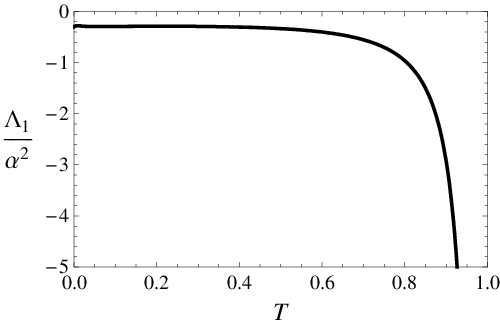
These two parameters do not depend on the number of hierarchical levels used. We remind that $\chi_{1}=q_{EA}-q$. The values of the temperature and the magnetic field are taken from the SK solution. Parameter $m$ is of order unity even at the boundary of the spin-glass phase (AT line) where the small parameter $\alpha$ vanishes. Its temperature dependence at the AT line is plotted in Figure 1.

The other parameter of the $1$RSB solution, $\chi_{1}$, is proportional to the small parameter $\alpha$ from Eq. (6g) and vanishes at the boundary of the spin-glass phase. Its ratio $\chi_{1}/\alpha$ at the AT line as a function of temperature is plotted in Figure 2.

The ratio diverges in zero magnetic field where $m=0$ and both $\chi_{1}$ and $m$ are linearly proportional to $\theta=(T_{c}-T)/T_{c}$, while $\alpha\sim 2\theta^{2}$ [11].

It is interesting to notice that the asymptotic solution near the AT line reduces to $1$RSB in non-zero magnetic fields. The SK solution can be asymptotically correct in the leading order only in zero field where the parameter $m_{1}=0$. In non-zero fields one has to go to $1$RSB even in the lowest asymptotic order below the instability line. The existence of the AT line hence indicates a replica-symmetry breaking. The instability in the magnetic field does not specify whether the discrete or the continuous RSB scheme applies in the low-temperature phase. Notice also that condition $\chi_{1}>0$ does not necessarily indicate a deviation from the SK solution. If $m_{1}=0$ then $q_{EA}=q+\chi_{1}=q_{SK}$. Only if both parameters $\chi_{1}$ and $m_{1}$ are simultaneously positive the physics of the SK solution is changed to $1$RSB.

To disclose the leading asymptotic behaviour of each separate parameter $\Delta\chi_{l}$ and $\Delta m_{l}$ for $l=1,\ldots,K$ we must go beyond $1$RSB and the leading orders in parameters $m$ and $\chi_{1}$. It is firstly the fourth order in $\alpha$ in Eq. (5) from which we find that $\Delta\chi_{l}\doteq\chi_{1}^{1}/K$ and

Both parameters $\chi_{1}$ and $\Delta m$ are linearly proportional to $\alpha$. The former, however, exists already in $1$RSB, while the latter first emerges in $2$RSB. Since they do not depend on the number of hierarchies used and determines a uniform distribution of parameters $m_{l}$ for $l=3,\ldots,K$, we demonstrated that all characteristic features of the asymptotic solution near the AT instability line are contained already in $2$RSB. What was, however, highly nontrivial was to unveil equidistant distributions of both parameters $\chi_{l}$ and $m_{l}$. Temperature dependence of the ratio $\Delta m/\alpha$ along the AT line is plotted in Fig. 3.

Finally we evaluated the instability conditions from Eqs. (6a) and (6b). They all coincide in the leading asymptotic order in $\alpha$. We find that all the discrete RSB solutions are unstable. Instability of the discrete scheme is measured by the small parameter $\alpha$. The SK ($K=0$) solution has the instability expressed via the AT condition

where $\Delta m$ was defined in Eq. (6jb). The difference in the order of magnitude in the instability of the SK and RSB solutions is caused by the existence of the non-zero parameter $m$ at the AT line where $\chi_{l}=0$. It is hence impossible for the SK solution without $m$ to reproduce the exact solution in the non-zero magnetic field even asymptotically with $\alpha\to 0$.

The stability conditions of the discrete RSB solutions manifest that only the continuous limit with $K\to\infty$ becomes marginally stable. The instability of $1$RSB is plotted in Figure 4. The leading-order term diverges at the critical temperature $T_{c}=1$, since the instabilities of the SK as well as of the discrete RSB solutions in zero magnetic field are proportional to $\alpha\propto(T_{c}-T)^{2}/T_{c}^{2}$ [11].

The basic assumption of the continuous limit of the discrete RSB scheme with the number of hierarchies $K\to\infty$ is a uniform distribution of the differences $\Delta\chi_{l}$. That is, they are independent of $l$ and are proportional to $K^{-1}$. We then can introduce a differential $dx=\lim_{K\to\infty}\chi_{1}/K$. It is not, however, necessary that all parameters $\Delta\chi_{l}$ are equal in the asymptotic limit $K\to\infty$ to end up in a continuous theory. The differences may vary by factors of order unity.

It is convenient to map the hierarchy indices $l$ on interval $[0,1]$ by introducing a continuous variable $x=\lim_{K\to\infty}(K-l)/K$. The continuous version of the hierarchical free energy results from a process in which we systematically neglect all higher than linear orders of the differential $dx$ [13]. It means that in the continuous limit we take into account only the second moments of the Gaussian integrations over the auxiliary fields $\lambda_{l}$. We first apply this procedure to the interacting free energy (2.1) and then to stationarity equations (3)-(5).

We denote $g_{l}\equiv\ln\mathcal{Z}_{l}$. Using the notation from the preceding section we obtain by cutting the expansion of Eq. (2) at the order $O(\Delta\chi_{l})$

We denoted $g_{l}^{\prime}\equiv\partial g_{l}/\partial h$. The derivatives with respect to the magnetic field stand for the action of the fluctuating field $\lambda_{l}$ when only the second moment contributes to the integral. In the continuous limit we obtain the Parisi differential equation by replacing the hierarchy index $l$ by the continuous variable $x$

We denoted $\dot{\chi}(x)\equiv d\chi(x)/dx$. The right-hand side of Eq. (6jkm) has opposite sign to the original Parisi equation, which is caused by a different assignment of the continuous variable $x$ to the hierarchy index. Parisi used $x^{P}=\lim_{K\to\infty}\ \ l/K$.

To derive the continuous limit of the stationarity equations we must first find a reduction of the density matrix $\rho_{l}$ in the limit of infinite hierarchical levels. Since only a linear term in $\Delta\chi_{l}$ contributes and the density matrix is normalised to unity we have

The operator of the derivative with respect to the magnetic field stands for the random variable $\lambda_{l}$. Integrals over this random variable of functions $f(\lambda_{l},h)$ weighted with the density matrix $\rho_{l}$ reduce in the continuous limit to

We need to evaluate multiple integrals over a number of random fields $\lambda_{l}$. We denote

The increment in the second index can again be represented in the continuous limit via a differential equation

The solution of the above equation can be represented in form of a ”time-ordered” exponential with differential operators [12]

The ordering operator $T_{y}$

orders products of $y$-dependent non-commuting operators from left to right in a $y$-decreasing succession. It is a standard tool used in many-body quantum theory to represent time-dependent perturbation expansion. It is easy to check that function $f_{x}(X,h)$ obeys Eq. (6jkpq).

With the aid of solution (6jkpr) we can represent any physical quantity in the continuous limit. First among them are the equations for the order parameters.

To derive an equation for the SK order parameter $q$ we simply put $f_{x}(0,h)=t(h)\equiv\tanh(\beta h)$. We obtain from Eq. (6jkpr)

Using this representation in Eq. (3) we reach at a generalisation of the SK relation

To evaluate the right-hand side of Eq. (4) we realise that

from which we find with the aid of integral representation (6jkpr)

We denoted $h_{\eta}=h+\eta\sqrt{q}$. Equation (6jkpv) is fulfilled for all $x\in[0,1]$. It essentially determines the functional dependence $\dot{\chi}(x)$. We know from the discrete scheme that $\dot{\chi}(x)>0$.

The last relation to be rewritten in the continuous limit is equation (5). It is not difficult to reach a representation

that now determines the functional dependence $m(x)$. Again from the discrete RSB scheme we know that $\dot{m}(x)<0$. The two functional equations (6jkpv) and (3.2) allow for a trivial solution reducing thereby the RSB quantities to the SK ones.

The derived equations for the continuous version of the order parameters from the discrete RSB scheme enable us to understand how we get rid of one functional order parameter. Namely, the function $\dot{\chi}(x)$ appears in all physical quantities only under integrals over the index variable $x$. We hence can redefine the differential $dx\to d\chi=dx\ \dot{\chi}(x)$, since $\dot{\chi}(x)>0$. We do not need to know the point-wise dependence $\dot{\chi}(x)$ to determine physical properties of the low-temperature spin-glass state. We hence can transform the defining interval $x\in[0,1]$ to a new one $\chi\in[0,X]$, where $X=\chi(1)\leq 1$. The largest value of $\chi(x)$ is the only parameter we need to know from this function. It must be determined from a stationarity equation and is related to the Edwards-Anderson parameter by an equation $q_{EA}=q+X$. When we resign on the explicit dependence $\dot{\chi}(x)$ we also have to disregard Eq. (6jkpv). Only stationarity equations for $q$ and $m(\chi)$, Eqs. (6jkpu) and (3.2), respectively, remain then relevant. They coincide with the equations derived from stationarity conditions imposed upon the Parisi free energy in Ref. [12].

Last but not least we have to find the continuous version of stability conditions (6a) and (6b). It is again straightforward to use the above results and integral representation (6jkpr) to arrive at

It was shown in Ref. [12] that equality in Eq. (6jkpx) can be derived from a total derivative of Eq. (3.2) with respect to variable $x$. It means that if equation (3.2) is fulfilled for all variables $x\in[0,1]$, both sides of Eq. (6jkpx) are equal as well. We thereby proved that the Parisi continuous RSB solution is marginally stable. The spin-glass susceptibility has zero eigenvalue but no negative ones.

We now explicitly asymptotically solve the equations for the order parameters of the continuous RSB scheme. We know from the discrete version that $\dot{\chi}(x)=1$ for $x\in[0,X]$ and vanishes elsewhere. We introduce a new dimensionless variable $\lambda=x/X$ that spans again interval $[0,1]$. The physical parameter $X$ serves as an expansion parameter in the asymptotic region near the AT instability line.

In the continuous limit we have two basic equations to solve. It is Eq. (6jkpu) for the SK order parameter $q$ and Eq. (3.2) from which we determine $X$ and $m(\lambda)$. It can be shown that for $x\leq X$ equation (6jkpv) is a total derivative of Eq. (3.2). There is thus no inconsistency if we disregard Eq. (6jkpv) as a stationarity equation for the free energy of the continuous RSB solution. We know from the preceding subsection that the total derivative of Eq. (3.2) with respect to $x$ expresses a marginal stability of the continuous RSB state.

The asymptotic solution near the AT line is a polynomial in variable $X$. We hence expand all quantities to a necessary order in this parameter. The $T$-exponential on the right-hand side of Eq. (3.2) must be expanded to $X^{3}$. Further on, the order-parameter function becomes also a polynomial in $X$. The relevant order parameters are then expanded as follows

We first use Eq. (6jkpu) to simplify Eq. (3.2) and then expand its right-hand side to $X^{3}$. Simultaneously we make use of the expansion of the order parameters from Eqs. (6jkpya) and (6jkpyb). We obtain a cubic polynomial in $\lambda$. Coefficients at each power of $\lambda$ must vanish and we have three equations for parameters $m_{0},m_{1}^{\prime}$ and $X$. Parameters $q_{1}^{\prime}$ and $q_{2}^{\prime}$ are determined from an expansion of Eq. (6jkpu). The explicit solution was calculated with the aid of the programme MATHEMATICA and reads

Here we denoted

The above solution is then used in the equations for $X,m_{0},m_{1}^{\prime}$. These three equations read

We determine $m_{1}^{\prime}$ from Eq. (6jkpyzaac), $m_{0}$ then from Eq. (6jkpyzaab). The two parameters we finally use in Eq. (6jkpyzaaa) from which we calculate $X$. To find the leading asymptotic behaviour of $X$ we have to expand it in powers of the initial small parameter $\alpha$ measuring the depth of penetration into the spin-glass phase. Parameter $\alpha$ was defined in Eq. (6g) and emerges in Eq. (6jkpyzaaa) as an absolute, $X$-independent term. The solutions for $X$ and $m_{0}$ from the continuous RSB scheme then coincide in the leading order in $\alpha$ with the result for $\chi_{1}$ and $m$ from the discrete $1$RSB solution, Eqs. (6i) and  (6h), respectively. The last parameter $m_{1}^{\prime}$ has an explicit representation

where again parameter $\Delta m$ was already determined within the discrete $2$RSB scheme in Eq. (6jb). The asymptotic limit of the full solution near the AT line is hence completely determined by the parameters from the two-step RSB solution.

References

- [1] Sherrington D and Kirkpatrick S 1975 Phys. Rev. Lett.35, 1972
- [2] Parisi G 1980 J. Phys. A: Math. Gen.13, L115, 1101, 1887
- [3] Parisi G 2007 Preprint arXiv:0706.0094v1 [cond-mat.dis-nn]
- [4] Guerra F 2003 Commun. Math. Phys. 233, 1
- [5] Talagrand M 2006 Ann. Math. 163, 221
- [6] Gross D J, Kanter I and Sompolinsky H 1985 Phys. Rev. Lett.55, 304
- [7] Janiš V 2005 Phys. Rev.B 71, 214403
- [8] Dotsenko V 2001 Introduction to the Replica Theory of Disordered Statistical Systems (Cambridge:Cambridge University Press).
- [9] de Almeida J R L and Thouless D J 1978 J. Phys. A: Math. Gen.11, 983
- [10] Janiš V 2006 Phys. Rev.B 74, 054207
- [11] Janiš V and Klíč A 2006 Phys. Rev.B 74, 054410
- [12] Janiš V 2007 Preprint arXiv:0711.1648v1 [cond-mat.dis-nn]
- [13] Duplantier B 1981 J. Phys. A: Math. Gen.14, 283