On the range of validity of the fluctuation theorem for stochastic Markovian dynamics
Abstract
We consider the fluctuations of generalized currents in stochastic Markovian dynamics. The large deviations of current fluctuations are shown to obey a Gallavotti-Cohen (GC) type symmetry in systems with a finite state space. However, this symmetry is not guaranteed to hold in systems with an infinite state space. A simple example of such a case is the Zero-Range Process (ZRP). Here we discuss in more detail the already reported [1] breakdown of the GC symmetry in the context of the ZRP with open boundaries and we give a physical interpretation of the phases that appear. Furthermore, the earlier analytical results for the single-site case are extended to cover multiple-site systems. We also use our exact results to test an efficient numerical algorithm of Giardinà, Kurchan and Peliti [2], which was developed to measure the current large deviation function directly. We find that this method breaks down in some phases which we associate with the gapless spectrum of an effective Hamiltonian.
,
1 Introduction
An important step in the understanding of non-equilibrium systems has been the development of so-called fluctuation theorems [3, 4] which quantify irreversibility by relating the probability of some “backward” process to that of a corresponding “forward” process. Formally, these fluctuation relationships all derive from a statement about the relative probabilities of a trajectory in phase space and the time-reversed trajectory. The various theorems found in the literature can be divided into two broad classes: transient relations (which are exact for finite times) and steady-state relations (which hold only asymptotically in the long-time limit)—see, e.g., [5, 6] for recent discussion of the various interconnections. In the present paper we will mainly be interested in asymptotic symmetries, specifically whether (or not) a given quantity satisfies a relation of the form
| (1) |
Here is the probability to observe, over time interval , a time-averaged value of some time-extensive quantity (e.g., entropy production). The symbol means logarithmic equality in the limit of large . In this paper, we refer to the relationship (1) as “the Gallavotti-Cohen fluctuation theorem” or simply “the fluctuation theorem”.
Historically, the concept of a fluctuation theorem emerged from computer simulations investigating the entropy production fluctuations in a sheared fluid [7]. A rigorous derivation of the form (1) was then given for the steady state of deterministic systems [8, 9] where the entropy-like functional can be identified with the rate of phase space contraction. Later proofs addressed stochastic dynamics [10, 11], leading to a general property of the large deviation function sometimes referred to as “Gallavotti-Cohen symmetry” (or GC symmetry for short). Here is associated with a current of some quantity through the system (e.g., the particle current in a lattice gas) and, for bounded state-space, the relation (1) holds for arbitrary initial condition. Recent work by Kurchan [12] has also explored how to recast the deterministic fluctuation theorem as the vanishing-noise limit of the stochastic one. In parallel to the theoretical development there has been much successful work on experimental verification of fluctuation theorems; for reviews see [4, 13, 14]. In particular, we note that recent experiments using an optical defect in diamond provide a simple realization of a two-state stochastic system [15, 16].
Very recently there has been considerable theoretical, experimental and numerical interest in cases where the symmetry (1) breaks down, see e.g., [17, 18, 19, 20, 1, 21, 22]. It is now understood that this effect can be attributed to certain boundary terms which become relevant in the case of infinite state space; see section 2 below for a detailed exposition in the context of stochastic Markovian dynamics. For deterministic systems, the effect of unbounded potentials was discussed by Bonetto et al. [20]. They argued for the restoration of the symmetry by removal of the “unphysical” singular terms. Earlier a similar phenomenon was found for a model of a trapped-Brownian particle treated via a Langevin equation [17, 23]. Within the Langevin framework, discussion of some related subtleties can also be found in [24, 25].
In [1] we provided a general discussion of this breakdown of Gallavotti-Cohen symmetry for many-particle stochastic dynamics within the context of a particular model—the zero-range process (ZRP). The ZRP plays a paradigmatic role in non-equilibrium statistical mechanics, hence such work offers a contribution to general understanding as well as providing concrete results for an important model. In the present paper, we give details of the analytical calculations leading to those results and compare them with direct evaluation of the current large deviation function using the recent algorithm of Giardinà, Kurchan and Peliti [2]. We also discuss some generalizations and present new results for the multi-site ZRP.
Interestingly, in the zero-range process, we do not find a constant value for the ratio of probabilities for large forward and backward current fluctuations. This is in stark contrast to analytical arguments [17, 20, 25] and numerical work [21] for other models. We argue below that the failure to observe this form of “extended fluctuation theorem” is due to strong correlations in our model between the boundary terms and the integrated current. These correlations persist even in the long-time limit; it would be interesting to see if effects of this type can be observed in any experimental situations.
The plan of the rest of the paper is as follows. First, in section 2, we give a general derivation of the Gallavotti-Cohen fluctuation theorem for stochastic systems and indicate also the relation to transient fluctuation theorems. Then, in section 3, we introduce our zero-range model and outline its treatment within this general framework. section 4 is devoted to a detailed calculation of the current large deviation function for the single-site version of this model, giving a concrete example of the breakdown of GC symmetry. In section 5 the analytical approach is complemented by use of the algorithm of [2] to obtain new numerical results for the large deviation function (and general insight into the applicability of the “cloning” method). Significantly, in section 6 we extend our discussion to larger systems, demonstrating how information about the current fluctuations in an -site ZRP can be obtained by mapping to an effective single-site model. Section 7 contains some conclusions and general perspectives.
2 The fluctuation theorem for Markovian dynamics
2.1 Central argument
Here we present a derivation of the fluctuation theorem for generalized currents of Markov processes defined on a finite configuration space. Our argument is based on that of [11].
Consider a continuous time Markov process which satisfies detailed balance in the stationary state. The system can be described by the transition rates from configuration to . In addition, consider a counter , the value of which increases by the amount at each transition . Here the matrix , which is required to be real and antisymmetric, can describe any type of real or abstract current in the system. As an example one can consider the particle current through a given bond: in this case is the number of particles hopping across the bond at a transition (which can be positive or negative depending on the direction of hopping). At the counter is set to zero; for any positive time it is a functional acting on the paths (sequences of configurations) from time to time and can be written as
| (2) |
Here is the number of configurations visited during time . In the following we refer to as the “time-integrated current” (or, where no confusion can arise, simply as the “current”). Note that, due to detailed balance, the mean of this current is always zero in equilibrium.
We define the driven system by the modified transition rates
| (3) |
from configuration to , where is a driving field conjugated to the specific current under consideration. In what follows we show that in this driven system the probability distribution function of the random variable satisfies the relation
| (4) |
asymptotically for large times, provided the state space (i.e., the number of possible configurations) is finite. Here the power can be interpreted as the work done on the system by the external field. This is the statement of the fluctuation theorem.
In cases where the sum gives zero for all periodic paths in the configuration space, becomes a simple function of the initial and final configuration, i.e., there is no real dependence on the history. In this special case not only the original but also the above-defined “driven” system would satisfy detailed balance in the stationary state. In the following we assume that this is not the case, i.e., there are periodic paths in the configuration space for which the sum is non-zero.
For a given non-equilibrium model with rates one can apply a reversed argument. In this case physically one can think of as a negative driving field, conjugated to the current under consideration, which is needed in order to “restore” detailed balance. If, for a specific value of , the rates (defined by (3)) lead to detailed balance then the fluctuation relation (4) holds for this current. This gives some freedom for the quantity which enters the fluctuation relation. The action functional of [11] ( in that paper) corresponds to the specific choice with , which leads to . These rates indeed lead to detailed balance, since for each pair of configurations the forward and backward transition rates are equal. This also implies that in the corresponding equilibrium distribution every configuration has the same weight.
Let us now define the rate for a full path as
| (5) |
where denotes the time when the transition from configuration to happened and corresponds to the overall exit rate from configuration . The conditional probability of such a path with transition times between and , provided at time 0 the system starts in configuration is . Using (3) one can readily show that
| (6) |
where is the time-reversed path of and is the equilibrium probability of configuration . In reference [26] the above relation is referred to as the “non-equilibrium detailed balance condition” with being the work done on the system. This also suggests the identification of as the work.
We note that in the case of discrete time dynamics the above scenario is very similar, the only difference is that here the quantities and denote transition probabilities rather than rates and the exponential factors in (5) are replaced by diagonal elements of the transition matrix .
2.2 Proof of the asymptotic fluctuation theorem for finite systems
In the calculation we use the so-called quantum Hamiltonian formalism where a basis vector is associated with each possible configuration and the state of the system (a probability measure on the configuration space) is denoted by a vector in this space with the normalization . Here is a row vector with components . In this formalism the master equation takes the form
| (7) |
which is similar to the Schrödinger equation in imaginary time. The transition rates are in the off-diagonal elements of and the conservation of probability requires
| (8) |
For more details on this formalism see [27].
As a first step of the proof we introduce the joint probability distribution function , which denotes the probability of being in configuration and having the value of the current at time . In what follows we calculate the generating function
| (9) |
where
| (10) |
The time derivative of is
| (11) | |||||
| (12) | |||||
| (13) | |||||
| (14) |
where is a modified Hamiltonian in which the transition rates corresponding to are multiplied by the factor . Note that is a non-stochastic matrix with for . Since is identical to the initial measure the generating function takes the form
| (15) |
The long-time behaviour of this quantity is characterized by the function
| (16) |
One finds from (15) that as long as the configuration space is finite, is given by the lowest eigenvalue of , since
| (17) |
Where are the eigenvalues and are the eigenvectors of . It is easy to show that is related to the large deviation function
| (18) |
of the time-averaged current through a Legendre transformation:
| (19) |
As a second step in the proof we show that has the symmetry property
| (20) |
where is a matrix with the equilibrium probabilities on the diagonal and zero elsewhere. For the rhs of (20) one finds
| (21) |
which leads to
| (22) |
for the non-diagonal elements of equality (20). Using (3) and the fact that the matrix is antisymmetric, the above condition takes the form
| (23) |
which is just the detailed balance condition for the equilibrium system and is trivially satisfied. This proves the relation (20) (The diagonal part of both the lhs and rhs is just the diagonal part of the original non-equilibrium Hamiltonian.)
2.3 Transient fluctuation theorem
The relation (4) is true only asymptotically, for large times. However, due to the symmetry (20), one can show that for specific initial conditions it can be made exact for any finite time. Namely, taking the equilibrium distribution as the initial condition then for the generating function one finds
| (26) | |||
| (27) |
This implies that the relation (4) holds exactly for any finite time (but only for this specific initial condition). This is the statement of the transient fluctuation theorem of Evans and Searles [28, 29, 3].
2.4 Boundary terms
As mentioned above, in a non-equilibrium system one has some freedom to choose the current to be considered. Here we investigate whether two different choices really give two independent relations for the fluctuations of the non-equilibrium system. In order to satisfy the conditions of the theorem, by applying field in the non-equilibrium model one should get back to detailed balance, which can be formulated as
| (28) |
Here is the energy of configuration in the equilibrium system. Taking the logarithm of (28) and summing up for a path results in
| (29) |
where is the action functional of [11] and is the potential in the initial (final) state. This shows that any two currents (that satisfy the conditions of the fluctuation theorem) differ only in boundary terms. In finite systems these terms are bounded, consequently their contribution to the net current is negligible in the limit, where . In these systems the fluctuation theorems for different currents give essentially the same information.
In order to demonstrate this, consider a driven exclusion process on a finite lattice. Here the number of possible configurations is clearly finite. There are many ways of defining the integrated particle current in the system: one can consider the current through a given bond, take a space-averaged current or measure the distance travelled by a tagged particle (in periodic systems). All these definitions give a different current for finite times but in the limit they are essentially the same, since the difference between them is bounded while they are proportional to .
However, for systems with infinite configuration space this argument does not hold and the boundary terms can be relevant even for large times, leading to several independent relations for the fluctuations.
The fact that the difference between two currents can be written as a boundary term suggests that the same holds for the difference between two initial states. Suppose that the transient fluctuation theorem holds for with the initial measure . Since for any two currents , the transient fluctuation theorem holds for any current with a boundary term as
| (30) |
where is the equilibrium potential corresponding to the current and with being the initial measure ( satisfies the theorem with ).
2.5 Breakdown of the fluctuation theorem in infinite systems
For infinite systems the above argument breaks down at (17), where one identifies defined in (16) with the lowest eigenvalue of . In cases where is infinite-dimensional, there is no guarantee that the scalar products appearing in (17) are finite. An explicit example of this breakdown is given in [1] and will be discussed in detail below. Note however, that the derivation of the transient fluctuation theorem still holds even for infinite systems. Consequently, a violation of the asymptotic fluctuation theorem requires the unbounded growth of the boundary term in (30).
To avoid possible confusion, we remark here that in the original dynamical systems formulation [8, 9] of the GC symmetry, a critical value already appears above which the relation (1) does not hold. This is a direct consequence of the fact that the large deviation function (equivalent to in our notation) diverges outside a finite interval. In contrast, in the stochastic framework of this paper, we consider situations where the large deviation function is always finite (i.e., formally ) but the symmetry may still have a restricted range of validity due to the relevance of boundary terms. Indeed, it has also recently been understood in the dynamical systems context, that adding singular boundary terms to a system with finite leads to a further reduction in the symmetry regime, see [20].
2.6 Extended fluctuation theorem
The argument we present in this section is largely based on that of van Zon and Cohen [17, 23], where they describe a generic scenario for the breakdown of the fluctuation theorem in the context of Langevin dynamics. This leads to an “extended fluctuation theorem”, where the quantity is linear for small (as suggested by the fluctuation theorem) but, after an intermediate crossover regime, saturates to a constant value for large . Similar arguments are also given in [25].
Our starting point is equation (30) which we now write for the time-intensive quantities:
| (31) |
Here is the corrected current for which the fluctuation theorem holds, and is a boundary term, which depends only on the initial/final configuration of the history.
First we assume that the probability distribution of has an exponential tail for very large/small values of :
| (32) |
Here we set to infinity if is bounded from above/below. Focusing on the case where the initial state is the steady state, one can assume that the probability distribution of is identical for the initial and final state, moreover, for large measurement times they become independent. This implies that the probability distribution of
| (33) |
is of the form
| (34) |
where .
As a next step we assume that and as random variables are independent. In this case the large deviation function of the fluctuations of are determined by
| (35) |
Here , which describes the large deviations of , satisfies the fluctuation theorem, i.e., . In figure 1, one can see how can be obtained from graphically by using (35). The points and are defined as those values of where the derivative of the convex function becomes and respectively. Outside the interval the function is linear with slope . Consequently, the quantity is linear from zero to , and after a crossover regime it saturates at to a constant value . We remark that in the case where is symmetric with respect to (e.g. in the case of Gaussian fluctuations) .
In a more general situation, where the initial state is not stationary, the fluctuations of are different in the initial and final state (we still require that the tails are exponential).
| (36) |
In this case the large deviations of take the following form:
| (37) |
where and . This leads to a variant of the extended fluctuation theorem, where the the quantity does not saturate but becomes linear with a non-zero slope for large .
We stress that the above argument relies strongly on the assumption that the boundary terms are independent of the bulk contribution. There are various examples in the literature where this holds, and the above extended form of the fluctuation theorem was found, e.g., [23, 17, 21]. In contrast, in the remainder of this paper, we discuss a simple stochastic Markovian system where there is a strong correlation between the boundary and bulk terms and hence this extended fluctuation theorem is not expected to hold.
3 Zero-range process
Here we demonstrate how the general formalism of the preceding section is applied to a specific model—the zero-range process (ZRP). First introduced by Spitzer in 1970 [30], the ZRP now plays a paradigmatic role in non-equilibrium statistical mechanics, see [31] for a recent review. In particular, for certain choices of parameters the model exhibits a condensation transition [32, 33] in which a macroscopic proportion of particles pile up on a single site. Condensation phenomena are well-known in colloidal and granular systems [34] and also occur in a variety of other physical and non-physical contexts [31].
3.1 Model
We study the one-dimensional partially asymmetric zero-range process with open boundaries [35]—see figure 2.

Each lattice site can be occupied by any integer number of particles, the uppermost of which hops randomly to a nearest neighbour site after an exponentially distributed waiting time. In the bulk particles move to the right (left) with rate () where is a function of the number of particles on the departure site ( by definition). Note that would correspond to free particles whereas all other forms represent an attractive or repulsive inter-particle interaction. The top particle on the leftmost lattice site (site 1) leaves the system with rate whereas new particles are injected with rate . Correspondingly, on the rightmost site (site ) particles are removed (injected) with rates (). For later convenience we label each bond by the site at its left-hand end, i.e., the th bond is between sites and .
In the quantum Hamiltonian formalism this dynamics is encoded in the Hamiltonian
| (38) | |||
| (39) |
where and are infinite-dimensional particle creation and annihilation matrices
| (40) |
and is a diagonal matrix with the th element given by .
3.2 Stationary state, current fluctuations
The steady state of the ZRP is given by a product measure (in other words, the stationary distributions for each site are uncorrelated):
| (41) |
where is the probability vector with components
| (42) |
Here the empty product is defined equal to 1 and is the local analogue of the grand-canonical partition function
| (43) |
The fugacities are uniquely determined by the hopping rates , , , , and . However, for bounded (i.e., with ), has a finite radius of convergence. For parameters leading to fugacities outside this radius of convergence, a growing boundary condensate occurs [35].
We are interested in the application of the fluctuation theorem to this model, for the case where the boundary parameters are chosen to give a well-defined steady state, i.e., without boundary condensation. As discussed in the preceding section, one can consider a variety of different “currents” through the system. However, since the state space is unbounded (each lattice site can contain an arbitrarily large number of particles) we anticipate the possibility of relevant boundary terms and different fluctuation relationships.
A natural choice is to look at the physical current of particles across a particular bond. For example, suppose we choose to focus on the particle current into the system (i.e., across the th bond), then the modified Hamiltonian is given by
| (44) |
In the next section we will examine closely the spectrum of this Hamiltonian for the single site case. Here we recap some known results for the general -site case as obtained in [36].
If is unbounded, (i.e., ) then has a gapped spectrum for all with lowest eigenvalue given by11 1 The leading order term in an expansion for the bulk-symmetric case, corresponding to the limit in (45), has also been obtained by an additivity principle [37] and by field-theoretic methods [38].
| (45) |
The right eigenvector corresponding to (45) has the same form as the stationary product measure (41) with fugacities
| (46) |
and the left-hand eigenvector is also a product state with one-site marginal “fugacities”
| (47) |
Note that this result is independent of the details of and one can also show that it is the same for currents across all bonds meaning that the current fluctuations are spatially homogeneous in the long-time limit. Furthermore the scalar products appearing in equation (17) are finite and the standard Gallavotti-Cohen fluctuation theorem is recovered. Physically, unbounded means that there is no chance for the temporary accumulation of a large numbers of particles on any site.
However, if is bounded, then there is a crossover to a gapless spectrum at some value of and also the scalar products in equation (17) can be infinite. In fact, and are related to the distribution of initial and final boundary terms and the condition for to diverge obviously depends on the initial state. Thus, although the symmetry of the eigenvalues remains, we expect the breakdown of the usual Gallavotti-Cohen fluctuation theorem in a spatially homogeneous and initial-condition-dependent way. To explore this issue in more detail we present, in the next section, explicit calculations for the single-site case.
4 Analytical results for single-site model
As a simple example of the ZRP with bounded , we now focus on the single-site model with —see figure 3.

Even this apparently simple model exhibits a rich phase behaviour, as shown in [1]. One must now distinguish between the particle currents across only two bonds viz. the 0th (“input”) and 1st (“output”). Since fluctuations across the two bonds are simply related by left-right reflection, we will consider only the former except where explicitly stated otherwise. Note that the occupation number of the site performs a random walk on a semi-infinite lattice but with two independent processes for movement in each direction. For a well-defined steady state this random walk should be biased towards the reflecting boundary at , i.e., we require . If this condition is not met then there is a growing condensate on the site.
Let us first consider an initial Boltzmann distribution given by
| (48) |
where denotes the configuration with site occupied by particles (i.e., a column vector with a ‘1’ in the th position and ‘0’s elsewhere) and the “fugacity” is less than 1 for normalization. For example, the choice is the steady-state initial condition. Note also that the limit corresponds to the empty-site case and that by ergodicity this gives the same result as any fixed particle configuration.
To obtain the large deviations of input current, we need to calculate the matrix element where the modified Hamiltonian is given by
| (49) |
In appendix A.1, we first present an explicit calculation of the spectrum of and thereby illustrate the crossover to a gapless regime. Then, in appendix A.2, we show how to obtain an integral representation of the matrix element and thus extract the large deviation behaviour. This enables us to construct and explain the “phase diagram” for current fluctuations as shown in section 1. Finally, in 4.3 we discuss some straightforward generalizations of these results.
4.1 Phase diagrams
In order to extract the large-time behaviour from the integral representation (110) we can use the method of steepest descents with saddle-point at . However, care must be taken due to the poles in the integrands (at , , and ). If the saddle-point contour has to be deformed through one of these poles then we must take into account the contribution of the residue at that pole. For a given , is then determined by the term which decays most slowly with . This yields changes in behaviour at the values of given in table 1, where we have defined for convenience the parameter combination
| (50) |
| Values of | Corresponding values of |
|---|---|
| , | |
| , |
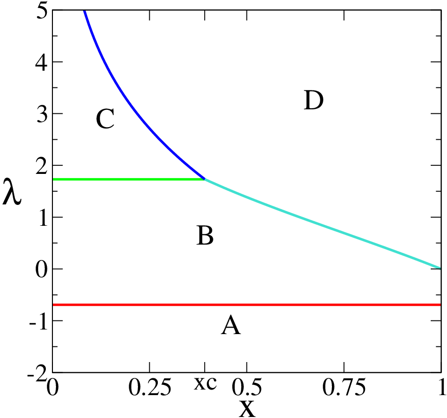
- Phase A:
- Phase B:
, where we defined as
(52) (see figure 4). In this region the spectrum of is gapped and coincides with the lowest eigenvalue:
(53) The quantities and are finite.
- Phase C:
(see figure 4). In this phase the spectrum of is gapless. The scalar products and are finite (here , which is the ground-state of , has to be understood as ), consequently is given by the lowest eigenvalue:
(54) - Phase D:
(see figure 4). In this phase the quantity diverges and differs from the lowest eigenvalue of :
(55) It is interesting that here the large deviation of current fluctuations retains a dependence on the initial state of the system.
For the physical interpretation of these phases it is better to consider , which can be obtained from by a Legendre transformation. has the following forms in the different regions of figure 5:
| (56) |
with
| (57) |
We remark that has a simple physical meaning. Consider a single particle performing a simple random walk on the infinite one-dimensional lattice with right (left) hopping rate (). Then the large deviation function of the distance travelled by this particle is given by .

In phase A only the rates for the first bond determine the large deviation function. For such large currents particles typically pile up on the site, which then acts as an infinite reservoir. In this case the behaviour of the two bonds decouples, so the current distribution across the input bond is entirely controlled by the two Poisson processes at rate and . This explains the first line in (56). The fact that in these (very unlikely) realizations the occupation number increases with time, is consistent with the divergence of . In stochastic systems such divergence is usually associated with the lack of a steady state. Here, the model does have a steady state so that realizations involving piling-up of particles (condensation) are never observed in the infinite time limit. However, as indicated, they characterize the fluctuations that can be observed over a large but finite measuring period . We therefore use the term “instantanous condensate”.
In phase B, which always contains the mean steady-state current (), the four rates enter symmetrically in the large deviation function. Note that the combinations and are the effective renormalized hopping rates of two exclusion particles with left (right) hopping rates () and (), in the case where they form a bound state [39]. In this regime the occupation of the site, which maps to the distance between the two exclusion particles, remains finite. The existence of this “two-particle bound state” is also manifested in the gapped spectrum of .
Although the naive approach (i.e. identifying with the lowest eigenvalue of ) still works in phase C, the large deviation function takes a different form here. For these large negative currents (and small initial occupation) it is needed that the current across the other bond also takes a large negative value (unlike in phase A). It can be seen in (56) that the contribution of the two bonds factorize suggesting that they act independently. This can be traced back to the change in the spectrum which becomes gapless in this regime, corresponding to a two-particle unbound state. The distance between the two particles (or equivalently the occupation of the site) grows as the square-root of time in such realizations—again we refer to this temporary piling-up as instantaneous condensation.
Phase D is in some sense the counterpart of phase A. Typical realizations contributing to these exponentially small probabilities start at a very high occupation (initial condensate) which then decreases during the observation time. For fixed , this is possible only for sufficiently large values of . This initial singularity is indicated by the divergence of .
One can see in the – phase diagram (see figure 5) that in between phases A–B and B–D transition regions appear. These regimes correspond to a single transition line in the – diagram along which the derivative of is discontinuous. This is entirely analogous to ordinary equilibrium phase transitions where different thermodynamical potentials are Legendre transforms of each other and in certain phase diagrams mixed regions (e.g. liquid–gas) appear at first order phase transitions lines. For the full analogy one can consider the following identifications: (specific) volume; pressure; Helmholtz free energy (density); Gibbs free energy (density). One can immediately see that the analogue quantity of the system size is the measurement time in our model which must diverge if a true phase transition is to exist. In the mixed regions of the phase diagram the system segregates in time, i.e., for some finite fraction of the whole measurement time the system behaves as being on one boundary of the mixed phase while for the rest of the time it switches to the other boundary.22 2 Mathematically speaking, knowledge of is only sufficient to determine where is differentiable. If is non-differentiable then is, in general, non-convex; Legendre transform of the non-differentiable points in then yields straight-line sections of the convex envelope of . However in our case, the physical argument based on phase separation in time, indicates that the linear sections obtained via Legendre transform do yield the correct form for in the transition regimes (i.e., the large deviation function is still convex). For a mathematical account of the subtleties of large deviation theory the reader is referred to [40]; the application to statistical mechanics is discussed in [41, 42].
One can formally consider as a space dimension. Then a path in the configuration space of the original model becomes a configuration of the new model, see e.g., [43]. If the original model has finite number of configurations then this leads to only one (diverging) dimension () in the new model hence no phase transition is possible in this case. Therefore for a real phase transition to take place one needs infinitely many possible configurations in the original model. In our single site model this is achieved in the simplest way.
The above analogy between ordinary equilibrium phase transitions and transitions in the large deviation function of current fluctuations suggests that the ordinary free energy can be considered as the large deviation function of density fluctuations, which is indeed the case. Vice versa, the large deviation of current fluctuations can be interpreted as some kind of “dynamical free energy”. The main difference between the two cases is that the pressure can easily be controlled and measured in an experiment, whereas that is not the case with . So far it seems that the only way to make measurements for or is the highly inefficient method of measuring the probabilities of large current fluctuations in a system where (zero pressure). However in the next section, we will see that with the help of a neat trick becomes adjustable in computer simulations. Still, the question of the (experimental) physical interpretation of this parameter remains open.
4.2 Range of validity of GC symmetry
Armed with the detailed knowledge of the phase diagram for our single-site model, we now return to the original question of the validity of the fluctuation theorem. For the GC symmetry to hold for currents of magnitude , we require that both and are in phases B or C (in which is given by the lowest eigenvalue of ). This immediately implies that the symmetry is seen only in the restricted interval where
| (58) |
This is shown as the shaded regime in figure 5. Note that depends on the initial distribution and that the GC symmetry is not seen at all above some critical value of .
Now let us investigate the ratio of probabilities for forward and backward currents outside the symmetry regime. For non-zero , then one sees a crossover to
| (59) | |||||
| (60) |
In other words, for large , the quantity is linear with slope . At first glance, this may appear to be the extended fluctuation theorem of section 2.6. However, the slope of the linear section is not as predicted there—in particular, it is not zero for an initial steady-state distribution (i.e., the ratio of forward and backward currents does not saturate to a constant value). We emphasize also that itself does not become linear for large as it does in the case of boundary terms which are independent of the bulk contribution. It would be interesting to develop a general argument to predict the behaviour in cases, such as this, where correlations are important.
4.3 Generalizations
Although the calculations of appendix A and section 1 were for a single-site model with the rates and a Boltzmann initial distribution (48) we argue here that they also have implications for more general single-site models.
Firstly, we note that results for the case where is any finite positive constant are trivially given by rescaling and . More generally, we argue that for the long-time behaviour only the large- asymptotics of are relevant and thus the results for any bounded function are obtained by the same rescaling of and . To see this note that the lowest eigenvalue in the gapped state (45) is independent of and the condition for occurrence of instantaneous condensates (divergence of the scalar products) depends only on the behaviour for as does the asymptotic current distribution out from such an instantaneous condensate. However the convergence to the long-time limiting behaviour is expected to depend on the form of making direct comparison of finite-time simulation results difficult.
By a similar argument, we expect any initial distribution with the same large- behaviour to lead to the same current large deviations. Since the elements of the lowest eigenvector fall off exponentially with , this means that any initial distribution with super-exponential decay should give the same result as the empty initial site (or any other fixed initial configuration), i.e., . Similarly, if the weight of configurations in the initial state decays slower than exponentially, then this corresponds to the case .
Finally, we remark that results for the current across the output bond can always be obtained by the replacements: , , , , , i.e., by left-right reflection. In section 6 we discuss extensions to larger systems.
5 Numerical results for
In [1], the analytical prediction for was checked via direct Monte Carlo simulation. However, it is difficult to get high quality data for long-times since one is looking for exponentially unlikely events. In this section we demonstrate instead the application of a recent algorithm by Giardinà, Kurchan and Peliti [2] to calculate directly.
5.1 Cloning algorithm
The method is based on an alternative interpretation of (15). Here acts as the generator of some kind of time evolution. However, it cannot be an ordinary stochastic evolution operator since it does not satisfy the normalization condition (8), therefore it does not conserve probability. The idea is to consider an ensemble of identical systems (clones), where the number of “individuals” being in the same configuration is denoted by . Here the size of the “population” can vary in time, which means that there is no conservation law for the vector as it is not a probability vector anymore (). The off-diagonal elements of give the currents from one configuration to another. The fact that is not normalized means that the sum of the currents from a specific configuration into any other is not necessarily equal to the loss in that configuration. This means that individuals can reproduce (i.e. introduce another copy of the system prepared in the same configuration as the ancestor by increasing by one) or die at given rates, where this rate depends on the configuration , and is given by .
The process described above can easily be simulated by Monte Carlo methods. The quantity to measure is the average rate of growth of the whole population for large times, which directly gives . In practice however, one chooses a sufficiently large which is kept constant by renormalizing the size of the population after each “birth” or “death” (while keeping a record of growth). The method was originally introduced for discrete-time update (for details see [2]) but is straightforwardly modified to the continuous time case (see also [44]).
Note that does not give the full probabilistic description of the above-defined stochastic cloning process. The deterministic time evolution (often called rate equation) given by refers only to the averages in a large population (). Therefore, in order to obtain reliable results one has to reduce the possible fluctuations of the (cloning) process by choosing large .
In a modified version of the algorithm the mean (integrated) current is measured instead of the growth rate. This gives the derivative of , which can be then numerically integrated (with the fixed condition ). We note that, in this algorithm, descendants of a given clone inherit not only the configuration of the parent but also the actual value of the parent’s integrated current. The advantage of this modified algorithm is that it gives less noise.
5.2 Results for the one-site ZRP with empty initial condition
We performed the above programme for the one-site ZRP. Since is known exactly, this should be considered as a test of the cloning method. Results are shown in figure 6(a) for the case of an empty initial site. It can be seen that the resulting data points for and lie very close to the exact () results in phases A and B. However, in phase C there is a significant deviation and the difference decreases with increasing . A systematic analysis of the -dependence of the cloning method is still lacking so it is not obvious how to set the value of in general to provide a good balance between accuracy and simulation speed.
Our numerical results suggest that in the gapless phase the simulation could be very sensitive to the value of and could deliver unreliable results for the accessible range. We believe that this limitation of the cloning method is related to the gapless spectrum and would not show up in cases where the state space is finite.
Figure 6(b) shows the results of a modified cloning algorithm, where the derivative of was measured directly and then numerically integrated. Despite the smoother results the same type of discrepancy shows up in this version of the simulation.
In the stationary state of the cloning process (if it exists), the distribution of the occupation number of clones is expected to follow the ground-state of . We measured this distribution in a representative point of phase B (, ) and C (, ). Results are shown in figure 7-8. The measured distribution in phase B follows the one suggested by the theory. In phase C (gapless phase) however, there is a significant difference between the theory and the measurement. This suggests that in the gapless phase the algorithm fails to find the true ground-state, hence is systematically overestimated in the measurement. This is consistent with the results shown in figure 6. We note that in phases A and D there is no steady state of the cloning process.
As discussed above, the cloning method strongly relies on the assumption that the number of clones is infinite. It is highly non-trivial to determine what type of correction appears if is finite (as in computer simulations). Our numerical results show that this correction is much higher in the gapless phase. This is possibly due to the fact that with a finite number of clones one cannot recover the exact distribution but some fluctuations are introduced. In the case of a gapped spectrum the system has a strong tendency to the ground state, therefore these fluctuations are suppressed and do not play a crutial role as long as they are sufficiently small ( is sufficiently large). In the gapless case however, the relaxation to the true ground-state becomes slow and therefore, due to the fluctuations, states other than the ground state are also represented in the sample with a non-negligible weight (see figures 7-8).
It is also possible to define for finite time, which we denote by .
| (61) |
Since measurements can be made only for finite times, the corrections to are of great interest. It is relatively easy to calculate the finite-time corrections in the single-site model based on (110). In phases A-B-D the leading contribution comes from a pole which leads to an correction in . In the gapless phase C the leading contribution is given by the saddle point integration. Since the first order term vanishes here the dominant contribution gives in (110), which leads to a correction, where is some constant. We performed exact numeric calculations of by evaluating the integrals in (110) and this is in good agreement with our analytical findings. For details see figure 9.
5.3 Non-empty initial condition
It is, in principle, possible to start the system from any initial condition in the cloning algorithm. Ideally, one would hope that the method reproduces the exact results in this regime. However, since the number of clones is finite, the initial distribution has always a finite (although arbitrarily large) cutoff. Although this is a minor change in the initial distribution, it becomes crucially important when measuring large deviations. A long time measurement for an initial distribution with a finite cutoff gives the same results as for an initially empty lattice. For an initial distribution with exponential tails (the case that we consider) one would need number of clones in a measurement of length . This is practically unreachable for reasonably large . For this reason it is not surprising that the algorithm breaks down in the initial-state-dependent phase.
6 Larger systems
In this section we extend our discussion to larger systems in order to demonstrate the generality of the fluctuation theorem breakdown for the current fluctuations. We consider the -site zero-range process with parameters as defined in section 3 and take again (but expect qualitatively the same results for any bounded ). For definiteness we assume that the boundary parameters have been chosen to give a well-defined steady state with mean (“forward”) current to the right. Once again, we focus on the behaviour of current fluctuations across the input (“0th”) bond but indicate also how to extend our approach to treat the fluctuations across bulk bonds. In section 6.1, we first outline our general method, in particular the use of a powerful mapping to effective one-site systems. This leads to a statement about the regime of validity of the GC symmetry (section 6.2) and some comments on generalizations (section 6.3). Finally, in section 6.4, we give explicit results for a two-site system and make comparisons with numerical data.
6.1 General approach
We remind the reader that, for a ZRP of arbitrary size, one can rigorously calculate the lowest eigenvalue in the gapped phase of the modified Hamiltonian measuring the input current together with the associated left and right eigenvectors and . Details of the calculations are given in [36], pertinent results are summarized in section 3 above. In order to determine the limit of the GC symmetry one has to ascertain the values of at which the scalar products and diverge whilst keeping in mind that the divergence of the normalization of the gapped eigenvalue indicates the cross-over to a gapless regime. To determine the behaviour of current fluctuations when these scalar products diverge we can appeal to the heuristic argument based on instantaneous condensates.
This process is considerably simplified by relating the current fluctuations in an -site system to those in a one-site system with effective parameters. We note that with the definitions
| (62) | |||||
| (63) | |||||
| (64) | |||||
| (65) |
the lowest eigenvalue (45) in the gapped phase of the modified Hamiltonian for an -site system (44) can be written in the form
| (66) |
and the corresponding left and right eigenvectors are defined by fugacities
| (67) | |||||
| (68) |
In other words, the one-site marginal for site and the eigenvalue have exactly the same form as in the one site problem with effective and ( and ) determined by all the rates to the left (right) of . This fact relies on the product-state character of the lowest eigenvector of the modified Hamiltonian corresponding to the current being measured. Notice that, by construction, , , and . We also remark that the parameter combinations and are independent of and are equal to the left/right hopping rates of an particle bound state in the corresponding exclusion process. Equivalently, in current space we have
| (69) |
This important observation allows us to utilize the exact results already obtained for the one-site case to build up the phase diagram for an -site system.33 3 Although our results can be applied to large systems by taking the thermodynamic limit , this limit does not necessarily commute with the long-time limit . Our analysis therefore does not address the form of current fluctuations in a genuinely infinite system (taking the limit first, followed by ).
Recall that corresponds to the mean current. The asymptotic probability of seeing a current fluctuation larger than the mean is given by the behaviour of for negative. To determine the part of the phase diagram we carry out the following procedure:
- 1.
Start with and given by of (66).
- 2.
Decrease until diverges on one of the sites, which we label . From the one-site picture we immediately see that this will happen at
(70) with defined as in Table 1. Physically, we argue (just as in the single-site case) that this divergence corresponds to the “piling-up” of particles on site . For the current fluctuations (across the input bond) only depend on the part of the system to the left of site and we thus expect a crossover to
(71) which corresponds to a current large deviation function.
(72) Just as in the single-site case, is continuous but not differentiable at so the two phases in current space are separated by a linear transition regime whose explicit form is simply obtained from the effective single-site picture.
- 3.
Now, with such an “instantaneous condensate” on site , the left-hand part of the system looks just like a system of size with right-hand boundary rates and . We can then write down the new ground state in terms of redefined effective parameters , , and .
- 4.
- 5.
At some value of , (with a function of the effective parameters) diverges on site 1 and the large deviation function takes the form
(73) (74) (again with a linear transition regime in -space). In other words, for very large forward currents, only the hopping parameters across the input bond are significant.
In a similar fashion one can investigate what happens for currents smaller than the mean by increasing from zero. For simplicity, let us first take a fixed initial configuration so that is always finite. At , diverges on site , corresponding to a transition to a gapless phase. The minimum value of occurs at some (which depends on the parameters of the model) so we first see a crossover to
| (75) | |||||
| (76) |
In other words, to sustain a large backwards current we have an instantaneous condensate on site and the product of current distributions across the two independent parts of the system. For increasing backwards currents, one can then repeat the procedure for the two subsystems (each with redefined effective parameters), increasing and looking for the next site where diverges. Eventually, for very large backward currents we expect instantaneous condensates on all sites and a current large deviation function given by
| (77) |
For a distribution over initial configurations, the situation is more complicated but again we can make progress based on the effective one-site picture. For an initial particle distribution which is a product measure of Boltzmann distributions with site dependent fugacity , then will diverge on the th site at leading to a crossover to an initial-state dependent regime. If is the (initial-condition-dependent) value of corresponding to the minimum of then, for large initial fugacities we expect to find first a transition to
| (78) | |||||
| (79) |
Once again, we see a factorization of the asymptotic current distribution across the two sub-systems to the left and right of . In principal, one can try to build up the complete phase diagram by next checking for the divergence of on other sites as is further increased. Another scenario, for small initial fugacities, involves first a transition to a gapless phase and then a transition to the initial condition dependent phase when as a function of the redefined effective rates.
6.2 Range of validity of GC symmetry
The effective one-site picture provides an elegant way to summarize the range of validity for the GC symmetry in ZRPs of arbitrary size. By comparison with (58) and with the shaded regime in figure 5, we see that, for given initial fugacities , the symmetry relation for input current will only be obeyed in the following current range:
| (80) |
where is the value of at which takes its minimum value as a function of the effective rates given in (62)–(65). In the case where is positive for some then the symmetry will not be observed at all.
6.3 Further generalizations
We remark that the same condition as (80) should also apply for ZRPs with quenched disorder (i.e., with and bond dependent)—one needs only to determine the appropriate form for the effective rates. Indeed, building on the recent determination of the stationary state for such systems [45], we can show that the relevant parameter combinations are
| (81) | |||||
| (82) | |||||
| (83) | |||||
| (84) |
where () is the right (left) hopping rate across bond and by definition , , and . One can state (81-84) alternatively as a simple recursion relation:
| (85) | |||||
| (86) | |||||
| (87) | |||||
| (88) |
Not surprisingly, these are again the renormalized two-particle hopping rates.
We conclude this subsection by indicating how to extend our approach to treat the current fluctuations across other bonds. In this case, the effective parameters are unchanged, but in all sites to the left of the bond in question the fugacities (67) and (68) must be replaced by
| (89) | |||||
| (90) |
corresponding to the expressions for the output bond of a single-site system.
6.4 Example: Two-site system
In principle, the general approach outlined above can be used to determine the behaviour of current fluctuations in ZRPs of arbitrary size. However the implementation rapidly becomes tedious and the phase diagram complicated. Here, as a simple test case, we present results for a two-site system with empty initial condition ( for all ).
It is obvious that for any choice of parameters obeying , the system has a well-defined steady state (i.e., no boundary condensation). One also gets a stationary state if the conditions
| (91) |
and
| (92) |
are obeyed. These inequalities can easily be understood in the exclusion picture where the first two particles form a bound state with hopping rates and . The condition for the bound state of this and the remaining single particle is just (92).
For definiteness, in the remainder of the discussion we assume that the rates obey (91) and (92). In this case, as is decreased from 0, diverges first on site 2 (i.e., ). Similarly, as is increased from 0, also diverges first on site 2 (i.e., ). Appealing to the heuristic “instantaneous condensates” picture we then obtain the following different regimes for the current large deviation function.
| (93) |
with
| (94) |
Here the currents , and are as defined in Table 1; we label the phases in analogy to A, B and C in the single-site case and note that there are intermediate transition regions at the A2–A1 and A1–B crossovers. From the argument in 6.2 it is clear that the Gallavotti-Cohen symmetry should hold for small currents .
Finally, we compare the Legendre transform of (93) with results for obtained via the cloning algorithm (see section 5). As shown in figure 10,
we find excellent agreement except for where is given by the lowest eigenvalue of a gapless spectrum. Just as in the single-site case we attribute this to limitations imposed by the finite number of clones.
7 Summary
This paper focuses on the Gallavotti-Cohen (GC) fluctuation symmetry in the context of continuous-time Markov processes. In particular, it offers a contribution towards understanding the potential breakdown of this symmetry in systems with infinite state space. To set the scene for this, we first discussed how the symmetry is manifested for the large deviation function of currents in systems with finite state space. Our proof was based on that of Lebowitz and Spohn [11] (or Derrida et al. [46]) but slightly extends their work by considering more general currents. In the notational framework of this paper, the action functional of Lebowitz and Spohn can be obtained by choosing and the GC symmetry then holds for with . In this case, as shown in [11], can be interpreted as an entropy current.
The above-mentionned proof of the fluctuation relation holds only for systems with finite state space---in systems with infinite state space the GC symmetry can be broken44 4 We remark that an infinite state space is not a sufficient condition for a breakdown of the Fluctuation Theorem. A counterexample is the ZRP with unbounded as explained in section 3.2. In the spirit of van Zon and Cohen’s earlier work for Langevin systems [23, 17], we next recapitulated the ideas leading to an “extended fluctuation theorem” in which (for stationary initial state) the ratio of probabilities of given forward () and backward () currents approaches a constant for large values of . We argued that this particular form of breakdown relies on the independence of bulk and boundary contributions to the current. The central aim of this paper was to study analytically a simple model where this condition is not met—the partially asymmetric Zero Range Process (ZRP) on an open lattice [35, 36].
Specifically, we expanded on earlier results in [1], and showed in detail how to calculate the large deviations of the average particle current in the one-site ZRP. The phase behaviour of the large deviation function can be physically understood by considering the possibility for an arbitrarily large number of particles to pile-up on the site (“instantaneous condensation”). Even in this single-site case, the phase diagram (parametrized by the time-averaged current and the initial state) shows a complex picture with first and second order phase transitions. These transitions are analogous to ordinary equilibrium phase transitions since formally the current large deviation function can be considered as a kind of dynamical free energy functional. In general, the GC symmetry holds only in a restricted interval , where depends on the initial state. The relevant parameter of the initial state, which is denoted by , can be considered as a kind of initial temperature. For large values of the regime of validity of the fluctuation relation shrinks ( decreases) and reaches zero at a finite . According to the above interpretation, this means that above a critical initial temperature the fluctuation theorem does not hold, even for small currents.
Although the one-site ZRP might be thought to be oversimplified, it is very instructive and already exhibits most features of the multiple-site version, which we have also studied in detail. In particular, we developed a heuristic argument based on mapping to an effective one-site system and considering the appearance of instantaneous condensates. The phase diagram can, in principle, be derived for any number of sites but it becomes increasingly complicated. As an example we showed how the current large deviation function can be obtained for a two-site ZRP. Again the phenomenon of instantaneous condensation is the physical mechanism leading to a breakdown of the GC fluctuation theorem.
Outside the symmetry regime, we found that the behaviour is somewhat different to that predicted by the extended fluctuation theorem of van Zon and Cohen, presumably due to the correlations (between bulk and boundary terms) in our model. There are evidently still open questions relating to the characterization of the fluctuation behaviour of different systems beyond the limits of Gallavotti-Cohen symmetry. For example, in another recent work [47] it was shown that the distribution of work fluctuations for a Brownian particle with Lévy noise (i.e., infinite variance) do not even have a large deviation form. It might be interesting to look for analogues of the resulting “anomalous fluctuation theorem” in the present framework of many-particle dynamics described by a master equation.
Our analytical results also made it possible to test the recently proposed cloning algorithm [2] that measures the Legendre transform of the large deviation function directly. The strength of this method is its efficiency and relative simplicity. The algorithm reproduces our analytical results in several phases. However, there are notable deviations in a phase where the spectrum of , the effective Hamiltonian governing the current fluctuations, becomes gapless. Another weakness of the algorithm is that it is unable to capture the initial-state-dependence of the fluctuations. It is only the case of a fixed initial configuration that this method can safely be used. These observations call for the development of a novel numerical algorithm which would not break down in cases where the cloning method does. One possibility here would be to develop a transition path sampling method.
Appendix
Appendix A Analytical calculations for single site model
A.1 Spectrum
Naively, one expects that the large deviation of current fluctuations is given by the lowest eigenvalue of according to (15). For this reason, we here study the spectrum of (49). First we transform into the symmetric form
| (95) |
using the diagonal operator
| (96) |
The diagonalization of is easily done by a Fourier transformation. We introduce which determines the character of the spectrum as follows:
-
Here the spectrum is entirely continuous. The eigenvector corresponding to wave number takes the form
(97) and the corresponding eigenvalue is
(98) -
In addition to the above continuous spectrum a discrete band appears with
(99) Here this is the lowest eigenvalue, correspondingly the spectrum becomes gapped. Notice that .
We note that it is easy to prove that the above set is complete, i.e.,
| (100) |
The right and left eigenvectors and of can be obtained by applying the operator :
| (101) |
for . In summary, for the lowest eigenvalue (infimum of the spectrum) of we obtain
| (102) |
It can easily be seen that this expression satisfies the symmetry relation (24), since with .
A.2 Calculation of the large deviation function
As a first step we write
| (103) |
where is a row vector with a ‘1’ at the th position and ‘0’s elsewhere. Inserting a complete set of eigenvectors we can write this in the form
| (104) | |||
| (105) |
Here denotes the Heaviside function. Using the symmetry of the eigenvectors and eigenvalues in the contribution of the continuous part, the above integral can be rewritten in the form
| (106) |
After the substitution and using (97) we obtain
| (107) | |||
| (108) |
where by we mean based on the above substitution. In order to be able to perform the infinite sums in (108), we have to choose the contour of the integral carefully. In the first term of the integral there is a pole only at . Here we chose the contour to be a circle of radius (denoted by ). In the second term we deform the contour to run along a circle around the origin with infinitesimal radius (denoted by ). Notice that doing so, for we pick up a pole contribution at , which just cancels with the last term in (108) (since ). Finally we obtain
| (109) | |||
| (110) |
To obtain the large deviation function we need to study the limit of this integral as . This enables us to build up the phase diagram as shown in section 4.1.
References
References
- [1] R. J. Harris, A. Rákos, and G. M. Schütz. Breakdown of Gallavotti-Cohen symmetry for stochastic dynamics. Europhys. Lett., 75(2):227–233, 2006.
- [2] C. Giardinà, J. Kurchan, and L. Peliti. Direct evaluation of large-deviation functions. Phys. Rev. Lett., 96(12):120603, 2006.
- [3] D. J. Evans and D. J. Searles. The fluctuation theorem. Adv. Phys., 51(7):1529–1585, 2002.
- [4] F. Ritort. Work fluctuations, transient violations of the second law and free-energy recovery methods: Perspectives in theory and experiments. Sém. Poincaré, 2:195–229, 2003.
- [5] J. Kurchan. Non-equilibrium work relations. J. Stat. Mech., P07005, 2007.
- [6] R. J. Harris and G. M. Schütz. Fluctuation theorems for stochastic dynamics. J. Stat. Mech., P07020, 2007.
- [7] D. J. Evans, E. G. D. Cohen, and G. P. Morriss. Probability of second law violations in shearing steady states. Phys. Rev. Lett., 71(15):2401–2404, 1993.
- [8] G. Gallavotti and E. G. D. Cohen. Dynamical ensembles in nonequilibrium statistical mechanics. Phys. Rev. Lett., 74(14):2694–2697, 1995.
- [9] G. Gallavotti and E. G. D. Cohen. Dynamical ensembles in stationary states. J. Stat. Phys., 80(5–6):931–970, 1995.
- [10] J. Kurchan. Fluctuation theorem for stochastic dynamics. J. Phys. A: Math. Gen., 31(16):3719–3729, 1998.
- [11] J. L. Lebowitz and H. Spohn. A Gallavotti-Cohen-type symmetry in the large deviation functional for stochastic dynamic. J. Stat. Phys., 95(1–2):333–365, 1999.
- [12] J. Kurchan. Gallavotti-Cohen theorem, chaotic hypothesis and the zero-noise limit. J. Stat. Phys., 128(6):1307–1320, 2007.
- [13] O. Narayan and A. Dhar. Reexamination of experimental tests of the fluctuation theorem. J. Phys. A: Math. Gen., 37(1):63–76, 2004.
- [14] F. Zamponi. Is it possible to experimentally verify the fluctuation relation? A review of theoretical motivations and numerical evidence. J. Stat. Mech., P02008, 2007.
- [15] S. Schuler, T. Speck, C. Tietz, J. Wrachtrup, and U. Seifert. Experimental test of the fluctuation theorem for a driven two-level system with time-dependent rates. Phys. Rev. Lett., 94(18):180602, 2005.
- [16] C. Tietz, S. Schuler, T. Speck, U. Seifert, and J. Wrachtrup. Measurement of stochastic entropy production. Phys. Rev. Lett., 97(5):050602, 2006.
- [17] R. van Zon and E. G. D. Cohen. Extension of the fluctuation theorem. Phys. Rev. Lett., 91(11):110601, 2003.
- [18] N. Garnier and S. Ciliberto. Nonequilibrium fluctuations in a resistor. Phys. Rev. E, 71(6):060101(R), 2005.
- [19] M. Dolowschiák and Z. Kovács. Fluctuation formula in the Nosé-Hoover thermostated lorentz gas. Phys. Rev. E, 71(2):025202(R), 2005.
- [20] F. Bonetto, G. Gallavotti, A. Giuliani, and F. Zamponi. Chaotic hypothesis, fluctuation theorem and singularities. J. Stat. Phys., 123(1):39–54, 2006.
- [21] A. Puglisi, L. Rondoni, and A. Vulpiani. Relevance of initial and final conditions for the fluctuation relation in Markov processes. J. Stat. Mech., P08010, 2006.
- [22] P. Visco. Work fluctuations for a Brownian particle between two thermostats. J. Stat. Mech., P06006, 2006.
- [23] R. van Zon and E. G. D. Cohen. Extended heat-fluctuation theorems for a system with deterministic and stochastic forces. Phys. Rev. E, 69(5):056121, 2004.
- [24] J. Farago. Injected power fluctuations in Langevin equation. J. Stat. Phys., 107(3–4):781–803, 2002.
- [25] M. Baiesi, T. Jacobs, C. Maes, and N. S. Skantzos. Fluctuation symmetries for work and heat. Phys. Rev. E, 69(2):021111, 2006.
- [26] T. Taniguchi and E. G. D. Cohen. Onsager-Machlup theory for nonequilibrium steady states and fluctuation theorems. J. Stat. Phys., 126(1):1–41, 2007.
- [27] G. M. Schütz. Exactly solvable models for many-body systems far from equilibrium. In C. Domb and J. Lebowitz, editors, Phase Transitions and Critical Phenomena, volume 19. London: Academic Press, 2001.
- [28] D. J. Evans and D. J. Searles. Equilibrium microstates which generate second law violating steady states. Phys. Rev. E, 50(2):1645–1648, 1994.
- [29] D. J. Searles and D. J. Evans. Fluctuation theorem for stochastic systems. Phys. Rev. E, 60(1):159–164, 1999.
- [30] F. Spitzer. Interaction of Markov processes. Adv. Math., 5(2):246–290, 1970.
- [31] M. R. Evans and T. Hanney. Nonequilibrium statistical mechanics of the zero-range process and related models. J. Phys. A: Math. Gen., 38(19):R195–R240, 2005.
- [32] M. R. Evans. Phase transitions in one-dimensional nonequilibrium systems. Braz. J. Phys., 30(1):42–57, 2000.
- [33] I. Jeon, P. March, and B. Pittel. Size of the largest cluster under zero-range invariant measures. Ann. Probab., 28(3):1162–1194, 2000.
- [34] G. M. Shim, B. Y. Park, J. D. Noh, and H. Lee. Analytic study of the three-urn model for separation of sand. Phys. Rev. E, 70(3):031305, 2004.
- [35] E. Levine, D. Mukamel, and G. M. Schütz. Zero-range process with open boundaries. J. Stat. Phys., 120(5–6):759–778, 2005.
- [36] R. J. Harris, A. Rákos, and G. M. Schütz. Current fluctuations in the zero-range process with open boundaries. J. Stat. Mech., P08003, 2005.
- [37] T. Bodineau and B. Derrida. Current fluctuations in non-equilibrium diffusive systems: an additivity principle. Phys. Rev. Lett., 92(18):180601, 2004.
- [38] F. van Wijland and Z. Rácz. Large deviations in weakly interacting boundary driven lattice gases. J. Stat. Phys., 118(1–2):27–54, 2005.
- [39] R. Juhász, L. Santen, and F. Iglói. Partially asymmetric zero-range process with quenched disorder. Phys. Rev. E, 72:046129, 2005.
- [40] A. Dembo and O. Zeitouni. Large Deviation Techniques and Applications. Springer, 1998.
- [41] Y. Oono. Large deviation and statistical physics. Prog. Theor. Phys., 99:165–205, 1989.
- [42] H. Touchette. The large deviation approach to statistical mechanics. arXiv:0804.0327, 2008.
- [43] V. Lecomte, C. Appert-Rolland, and F. van Wijland. Thermodynamic formalism for systems with markov dynamics. J. Stat. Phys., 127(1):51–106, 2007.
- [44] V. Lecomte and J. Tailleur. A numerical approach to large deviations in continuous time. J. Stat. Mech., P03004, 2007.
- [45] O. Pulkkinen. Boundary driven zero-range processes in random media. J. Stat. Phys., 128(6):1289–1305, 2007.
- [46] B. Derrida, B. Douçot, and P.-E. Roche. Current fluctuations in the one-dimensional symmetric exclusion process with open boundaries. J. Stat. Phys., 115(3-4):717–748, 2004.
- [47] H. Touchette and E. G. D. Cohen. Fluctuation relation for a Lévy particle. Phys. Rev. E, 76:020101(R), 2007.