Highly Frustrated Magnetic Clusters: The kagomé on a sphere
Abstract
We present a detailed study of the low-energy excitations of two existing finite-size realizations of the planar kagomé Heisenberg antiferromagnet on the sphere, the cuboctahedron and the icosidodecahedron. After highlighting a number of special spectral features (such as the presence of low-lying singlets below the first triplet and the existence of localized magnons) we focus on two major issues. The first concerns the nature of the excitations above the plateau phase at of the saturation magnetization . Our exact diagonalizations for the icosidodecahedron reveal that the low-lying plateau states are adiabatically connected to the degenerate collinear “up-up-down” ground states of the Ising point, at the same time being well isolated from higher excitations. A complementary physical picture emerges from the derivation of an effective quantum dimer model which reveals the central role of the topology and the intrinsic spin . We also give a prediction for the low energy excitations and thermodynamic properties of the spin icosidodecahedron Mo72Fe30. In the second part we focus on the low-energy spectra of the Heisenberg model in view of interpreting the broad inelastic neutron scattering response reported for Mo72Fe30. To this end we demonstrate the simultaneous presence of several broadened low-energy “towers of states” or “rotational bands” which arise from the large discrete spatial degeneracy of the classical ground states, a generic feature of highly frustrated clusters. This semiclassical interpretation is further corroborated by their striking symmetry pattern which is shown, by an independent group theoretical analysis, to be a characteristic fingerprint of the classical coplanar ground states.
pacs
75.50.Xx,75.10.Jm,75.40.MgI Introduction
The field of highly frustrated magnetism has received a growing theoretical and experimental interest in recent years Misquish_Review_2D_AFM; Richter_chapter. One of the central motifs in the planar kagomé and similarly frustrated Heisenberg antiferromagnets (AFM’s) which readily differentiates them from unfrustrated (e.g. collinear) ones, is the proliferation of an extensive family of low-energy singlets below the lowest triplet excitation Lecheminant_kagome; Waldtmann. One interpretation for the origin of these singlets has emerged from Resonating Valence Bond (RVB) type of arguments Mila for the kagomé AFM. For higher spins, purely classical considerations assert that the singlets stem from the splitting by quantum fluctuations of the extensively degenerate family of Néel ordered (3-sublattice) ground states Moessner_Review_Class_Deg. Both interpretations rest on the notion of a local degeneracy which stems from the frustrated corner-sharing topology of these lattices. In this regard, it appears that the proliferation of singlets is only one particular manifestation of this local degeneracy since similarly dense low-energy excitations are manifested in the whole magnetization range.
On the other hand, some understanding for the ground state itself has been established. Exact Diagonalization (ED) results suggest that the ground state of the kagomé AFM is a disordered spin liquid with a very small spin gap Lecheminant_kagome; Waldtmann (if any). For , semi-classical approaches predict that an extensive subset of coplanar states is first selected in while the ordered state is stabilized in higher orders through the order-by-disorder mechanism Chubukov; ChanHenley. In a magnetic field, the ground state may exhibit a number of interesting phases. These include the presence of an extensively degenerate family of localized magnons which result in macroscopic magnetization jumps at the saturation field, as well as the stabilization of spin gaps and the associated fractional magnetization plateaux. For a first understanding of the nature of these plateaux a perturbative expansion around the degenerate Ising point was first employed by Cabra et al. Cabra for the kagomé. This approach was recently extended by Bergman et al. Bergman1; Bergman2 to other frustrated systems, such as the pyrochlore AFM. Here, the anisotropy terms are treated perturbatively, and the emerging splitting of the degenerate Ising manifold is effectively cast into a Quantum Dimer Model (QDM) on the dual lattice.
At the same time, it is well known that some precursors of the excitation spectra of frustrated and unfrustrated AFM’s are already embodied in the spectra of small system sizes (see for instance Ref. Lhuillier_Towers). It has come therefore with no surprise that a number of phenomena that are manifest in kagomé-like AFM’s have also emerged in the research field of highly frustrated nanomagnets GSV; Schnack_Review; Christian_Meta; Fe30_Plateau; Schmidt_Singlets; Schnack_ind_magn_MMs; Schnack_caloric. These are realizations of zero-dimensional molecular-size magnets which consist of a finite number of strongly interacting transition metal ions, with the isotropic Heisenberg exchange being the dominant energy term. Thus, in addition to their great relevance in the context of nanomagnetism and the growing interest for potential applications in quantum computing Appl_QC, information storage Appl_MS and magnetic imaging Appl_MI, molecular nanomagnets can also provide a suitable platform for addressing theoretical questions and testing ideas from the more general context of frustrated magnetism.


In this work, we focus on two magnetic molecule realizations of the Heisenberg kagomé AFM on the sphere. The first consists of corner-sharing triangles and is realized in the Cu12La8 Cu12 cluster with Cu2+ ions occupying the vertices of a symmetric cuboctahedron (cf.Fig. 1). The spin topology of this cluster is identical to the -site kagomé wrapped on a torus (cf. Fig. 16). The second cluster is one of the largest frustrated molecules synthesized to date, namely the giant Keplerate Mo72Fe30 system Muller_Fe30. This features an array of thirty Fe3+ ions occupying the vertices of twenty corner-sharing triangles spanning an almost perfect icosidodecahedron (cf.Fig. 1). Interestingly, its quantum analogue, Mo72V30, consisting of V4+ ions has also been synthesized quite recently V30_1; V30_2. We may note here that the cuboctahedron and the icosidodecahedron can be thought of as two existing positive curvature (with 4 and 5 respectively) counterparts of Elser and Zeng’s ElserZeng generalization of the kagomé structure on the hyperbolic plane where each hexagon is replaced by a polygon of sides with .
Among the above highly frustrated clusters, Mo72Fe30 has been the most investigated so far, both theoretically and experimentally. The exchange interactions in Mo72Fe30 are quite small, K Muller_Fe30, and this has allowed for the experimental observation of a plateau at Tesla which has been explained classically by Schröder et al. Fe30_Plateau. In addition, this cluster manifests a very broad Inelastic Neutron Scattering (INS) response as shown by Garlea et al. Garlea_INS. On the other hand, Mo72V30 has a much stronger AFM exchange K V30_1; V30_2, and thus is not well suited for the observation of the field-induced plateau. However, its low-energy excitation spectrum can still be investigated by INS experiments (which, to our knowledge, have not been performed so far). As to the cuboctahedron Cu12La8 Cu12, we are not aware of any magnetic measurements reported so far on this cluster.
The main magnetic properties of the present clusters can be explained very well by the isotropic Heisenberg model with a single AFM exchange parameter , i.e.
| (1) |
where, as usual, denotes pairs of mutually interacting spins at sites and . Other terms such as single-ion anisotropy (for ) or Dzyaloshinsky-Moriya interactions must be present as well in the present clusters, but they are expected to be much smaller than the exchange interactions and thus they can be neglected. Here, as a simple theoretical tool to understand some of the properties of the Heisenberg model, it will be very expedient to introduce some fictitious exchange anisotropy, i.e. extend Eq. (1) to its more general XXZ variant
| (2) | |||||
| (3) | |||||
| (4) |
where , denote the transverse and longitudinal exchange parameters respectively. In what follows we denote .
The main results presented in this article are of direct relevance to the experimental findings in Mo72Fe30 mentioned above and thus span two major themes. The first deals with the nature of the low-lying excitations above the plateau phase. For the icosidodecahedron we show that all these excitations are adiabatically connected to collinear “up-up-down” (henceforth “uud”) Ising ground states (GS’s), at the same time being well isolated from higher levels by a relatively large energy gap. We argue that this feature must be special to the topology of the icosidodecahedron and that it must survive for as well. This prediction can be verified experimentally by a measurement of the low-temperature specific heat and the associated entropy content at the plateau phase of Mo72Fe30. A complementary physical picture will emerge by performing a high order perturbative expansion in , in the spirit of Refs. Cabra; Bergman1; Bergman2, and by deriving and solving to lowest order the corresponding effective QDM on the dual clusters. The dependence of the model parameters on and is also found and given explicitly.
Our second theme concerns the origin of the broad INS response reported for Mo72Fe30 Garlea_INS. Previous theories based on the excitations of the rotational band model Garlea_INS; SchnackLubanModler or on spin wave calculations Cepas_LSW; Waldmann_LSW predict a small number of discrete excitation lines at low temperatures and thus cannot explain the broad INS features. Our interpretation of this behavior is based on the notion of the simultaneous presence of several rotational bands or towers of states at low energies which originate from the large degree of classical degeneracy, a generic feature of highly frustrated systems. Indeed, our exact diagonalizations demonstrate the existence of an unusually high density of low-energy excitations manifesting in the full magnetization range. A detailed group theory analysis reveals that the low-energy spectra are of semiclassical origin up to a relatively large energy cutoff. We will also show that the symmetry of the corresponding excitations for does not conform with this semiclassical picture.
A quite appealing feature of these molecular clusters is their high point group symmetry, namely the full Octahedral group (with 48 elements) and the full Icosahedral group (with 120 elements) for the cuboctahedron and the icosidodecahedron respectively (here denotes the inversion). This allows for a drastic reduction of the dimensionality of the problem. In order to fully exploit all symmetry operations we have employed a generalization nikos of the standard ED technique ED so as to treat higher than one-dimensional Irreducible Representations (IR’s) also. With this approach, one is able to classify the energy levels according to both and the IR of the point group while resolving their full degeneracy.
The remainder of the article is organized as follows. In Sec. II we discuss some of the spectral features of the present kagomé-like nanomagnets (with particular emphasis on localized magnons) and contrast them to typical spectra of unfrustrated AFM’s. This is illustrated by comparing with a simple 12-site bipartite cluster. The investigation of the nature of the plateau is presented in Sec. III. This includes both analytical and numerical results from high order degenerate perturbation theory around the Ising limit, the construction of the associated effective QDM’s and their extrapolation to the Heisenberg limit. We also discuss the case of higher and the connection to the plateau phase of Mo72Fe30. In Sec. IV we demonstrate the presence of several low-energy rotational bands in Heisenberg spectra and reveal their semiclassical origin. The analysis is based on a careful comparison to the symmetry properties of the semiclassical states and follows the basic lines of the seminal works of Bernu et al. Bernu1; Bernu2 and Lecheminant et al. Lecheminant_J1J2; Lecheminant_kagome on this subject in the context of the triangular and kagomé AFM. Predictions for the corresponding tower of states are also given for the () icosidodecahedron. Our core idea of the presence of several rotational bands due to the large spatial degeneracy of the classical states is also exemplified in Sec. IV.2 by a discussion of the much simpler case of the XY model. We leave Sec. V for an overview of the major findings of this work. In order for the manuscript to be self-contained, we include two appendices. In Appendix A we summarize the main aspects of the degenerate perturbation expansion around the Ising limit, while in Appendix B we give the details of the derivation of the full symmetry properties of the semiclassical towers of states for the Heisenberg and the XY model.
A special remark is in order here regarding our choice of presentation of the spectra. Since we are interested in the low-energy excitations in the whole magnetization range (these are the most accessible and thus most relevant as one ramps up an external field at low temperatures) and in order to best illustrate the central features, we have chosen to (except for Fig. 3) shift the lowest energy (or ) of each () sector to zero. This guarantees a fine resolution of the low-energy spectra in the whole magnetization range.

II Unfrustrated vs. kagomé-like AFM’s : General spectral features (s=1/2)
Our main purpose in this section is to present the low-energy spectra of the Heisenberg cuboctahedron and icosidodecahedron and to highlight their main features which are common in all frustrated AFM’s. For comparison, it is expedient to also present the energy spectrum of a bipartite unfrustrated magnet. To this end, we have chosen the hypothetical 12-site cluster depicted in Fig. 2. The symmetry of this cluster is the dihedral group which consists of 24 elements. Figure 3 shows the low-energy Heisenberg spectrum as a function of , classified according to the 12 different IR’s of (cf. Ref. GroupTheory) shown in the legend. The spectrum is typical of unfrustrated AFM’s Lhuillier_Towers; Richter_chapter of finite size . For instance, we may associate the lowest energy band indicated by the dotted line in Fig. 3 with the so-called Anderson tower of states Lhuillier_Towers, which is the finite-size manifestation of the symmetry breaking process occurring in the thermodynamic limit. As can be seen in Fig. 3, this tower consists entirely of the two one-dimensional representations A1g and B2g of , which alternate between even and odd respectively. The physics behind this symmetry structure is intimately related to the symmetry properties of the semiclassical two-sublattice Néel state. For instance, the combinations A1g B2g transform into each other in exactly the same way as the two spatial counterparts of the Néel state. Above the lowest tower of states of Fig. 3 there exists a finite excitation gap followed by a quasi continuum of higher excitations. All these features are typical of unfrustrated AFM’s.


In contrast, frustrated AFM’s show very different low-energy features as exemplified by the spectra shown in the two lower panels of Fig. 4 for the two molecular magnets of the present study. For comparison, the upper panel shows the low-energy portion of Fig. 3 in terms of . The contrast between the two types of spectra is more than evident (note that both of the upper two panels correspond to 12-site clusters and are shown in the same energy scale). The most striking feature emerging in frustrated AFM’s is the absence of a clear energy scale separating a lowest band from higher lying excitations. Instead, a large “bulk” of low-energy excitations is manifested in the whole range of forming a quasi-continuum. This is a central feature that holds also for higher (cf. Sec. IV) and stems from the highly frustrated exchange interactions in these clusters. The nature of these excitations for is not completely understood Mila but, as we are going to show in Sec. IV, a qualitative understanding can be obtained for based on the large classical degeneracy of spin configurations which remains dominant in the semiclassical regime. In particular, the broad INS response reported in Ref. Garlea_INS for Mo72Fe30 is naturally accounted for by the results of this analysis.
(a) cuboctahedron deg. deg. 0 -5.44487521 1 4 0 3 1 -5.06220685 3 5 3 5 2 -4.36867379 1 6 6 1 3 -2.63135381 1
(b) icosidodecahedron deg. deg. 0 -13.23421620 1 8 -4.80706643 4 1 -13.01640033 1 9 -2.41759676 1 2 -12.61867043 5 10 0.31845649 1 3 -12.05650773 1 11 3.12078845 1 4 -11.22383327 1 12 6 2 5 -10.30278977 5 13 9 25 6 -8.95866550 1 14 12 10 7 -7.01225008 4 15 15 1


Let us now describe shortly some special spectral features and their origin. The ground state energies for the two nanomagnets for are given in Table 1. These energies determine the zero-temperature magnetization processes shown in Fig. 5. For the excitations above the ground state, three regimes of special interest can be highlighted (see shaded areas in Fig. 4): (i) the singlet excitations below the lowest triplet11 1 The presence of these singlets has been revealed previously by the work of R. Schmidt et al. in Ref. Schmidt_Singlets but the exact numbers and degeneracies could not be resolved by the reduced symmetry ED method used there. which are given in Table 2 and amount to 7 for the cuboctahedron and 80 for the icosidodecahedron22 2 Quite interestingly, this number equals approximately which is quite close to the reported Waldtmann scaling of for the number of low-lying singlets in the kagomé (with even ) despite the fact that the icosidodecahedron contains pentagons and not hexagons., (ii) the existence of degenerate localized magnons below saturation and (iii) the presence of a number of well isolated low-lying states right above the () plateau phase of the icosidodecahedron. The latter will be analyzed in detail in Sec. III.
(a) cuboctahedron Energy [J] IR (deg) Energy [J] IR (deg) -5.44487521 A1u(1) -5.29823654 Eg (2) -5.32839240 A1g(1) -5.16529346 T1g(3)
(b) icosidodecahedron Energy [J] IR (deg) Energy [J] IR (deg) -13.23421620 Ag (1) -13.09125447 Hg (5) -13.18689258 Au (1) -13.08659708 Fg (4) -13.18057238 T1u(3) -13.07844898 Au (1) -13.15013156 Hu (5) -13.07310588 Fu (4) -13.14089964 Ag (1) -13.07200565 T1u(3) -13.14024171 T1g(3) -13.05645698 T2u(3) -13.12997109 Hu (5) -13.05072896 Hu (5) -13.12560855 T2g(3) -13.04261651 Fg (4) -13.12514475 T2u(3) -13.03366847 T2g(3) -13.11552338 Hg (5) -13.02470946 Fg (4) -13.10136600 Fu (4) -13.02203094 Hg (5) -13.09264778 Hu (5)
The concept of localized magnons has been largely discussed in the context of highly frustrated bulk AFM’s Richter_chapter; Schulenburg_ind_magn; Schmidt_ind_magn; Derzhko_ind_magn; Schnack_ind_magn_bulk; Richter_JPhys; Mike_Caloric. For the present clusters it has been discussed by Schnack et al. Schnack_ind_magn_MMs; Schnack_caloric. We shortly revisit this issue here in the light of our symmetry resolved method. Quite generally, the eigenvalues of in the one magnon () subspace are equal (apart from an overall constant energy shift) to the eigenvalues of the adjacency matrix times the spin SchmidtLuban. Our decomposition of the respective subspaces for the cuboctahedron and the icosidodecahedron in terms of IR’s of the full and groups are (in order of increasing energy): (EgT2u)T2gT1uA1g, and (HgHu)T2uFgFuHgT1uAg respectively, and they are compatible to the ones given in Ref. SchmidtLuban in terms of IR’s of the and subgroups.

For the cuboctahedron, the lowest one-magnon level is 5-fold degenerate (EgT2u), see Fig. 4(middle). These correspond to localized, non-interacting magnon states. The smallest loops that can host such magnons are the square faces depicted in Fig. 6(a). The 5-fold degeneracy is due to the fact that there are 6 different square faces on this cluster, but not all magnons are independent: The sum of all 6 square magnons taken with opposite phases in neighboring squares vanishes. The lowest energy level of the two-magnon space is 3-fold degenerate (AgEg), and corresponds to the 3 different ways of placing two non-interacting magnon excitations (there are three different pairs of opposite squares). Placing one more magnon gives an interaction energy cost and a non-degenerate lowest level. We should remark here that magnon states “living” on the hexagonal equators of the cluster are also exact eigenstates, but each of these can be easily expressed as a linear combination of surrounding square magnons. The lowest level degeneracies for the one-magnon and the two-magnon space are in agreement with the values of and respectively with which are derived in Ref. Derzhko_ind_magn for the kagomé lattice (for which the hexagonal loops are the most local and natural ones for the description of the localized magnons).
For the icosidodecahedron, the lowest one-magnon level is 10-fold degenerate (HuHg). Here, the smallest loops that can host such localized states are the octagons surrounding a given vertex and depicted in Fig. 6(b). The 10-fold degeneracy can be attributed to a non-trivial linear dependence among the 30 different octagonal magnons on this cluster. The lowest energy level of the two-magnon manifold is 25-fold degenerate and decomposes into . Hence, there exist 25 ways of placing two mutually non-interacting magnons. Similarly, the lowest energy of the three-magnon space is two-fold degenerate (AgAu), whereas that of the sector is non-degenerate, signifying that it is not possible to have four magnons without an interaction energy cost.
The existence of localized, non-interacting magnon states results in a magnetization jump of , since the lowest energies at the corresponding sectors scale linearly with the number of magnons, and thus cross each other at the same (saturation) field. We remark here that all features related to the existence of localized magnons (symmetry decomposition, degeneracy, and the magnetization jump in absolute units) do not depend on the value of (see e.g. Fig. 14 below). Finally, the fact that the number of independent magnons is larger in the icosidodecahedron than the cuboctahedron case is clearly related to their size. In extended frustrated AFM’s, this number grows exponentially with system size but depends in a non-trivial way on the topology of the system and is connected to the question of linear independence Schmidt_ind_magn; Derzhko_ind_magn. The extensive degeneracy gives rise to a macroscopic magnetization jump at the saturation field and a large magnetocaloric effect (see e.g. Ref. Mike_Caloric). A study of the latter on the present clusters can be found in Ref. Schnack_caloric.
III Plateau phase
In this section, we focus on the nature of the excitations above the plateau. There are two major reasons for paying special attention to this particular plateau among the remaining ones which are present anyway in our finite-size clusters (cf.Fig. 5). The first is of practical interest and is related to the experimental manifestation Fe30_Plateau of this particular phase in the Mo72Fe30 cluster. Besides, as shown in the upper panel of Fig. 5, the plateau seems to be the most stable and survives at finite (the staircase magnetization process eventually turns into the expected (classical) linear behavior Fe30_Plateau for very large ). The second reason is that the plateau phase is a generic feature of frustration and is known to survive in the thermodynamic limit for some bulk AFM’s (cf. Ref. Richter_chapter).
In Sec. III.1 we present and analyze a striking feature of the excitations above the plateau phase of the icosidodecahedron and show how it can be observed experimentally in thermodynamic measurements. In Sec. III.2 we present our derivation of an effective Quantum Dimer Model for the plateau and reveal the major role of the topology and the spin .
| Energy [J] | IR(deg) | Energy [J] | IR(deg) |
|---|---|---|---|
| -10.30278978 | Hu (5) | -10.26904953 | Hu (5) |
| -10.29875816 | Ag (1) | -10.26657194 | Hg (5) |
| -10.29837409 | Hg (5) | -10.25765943 | Hg (5) |
| -10.29057364 | Fg (4) | -10.25604215 | Ag (1) |
| -10.28622445 | Fu (4) | -10.24060604 | Au (1) |

III.1 Thermodynamics
Our Exact Diagonalizations for the icosidodecahedron shown in the lowest panel of Fig. 4 reveal a striking feature at the sector: The low-lying excitation spectrum immediately above the plateau consists of a group of 36 states (their energies are given in Table 3) which are well isolated from higher excitations by a gap of order , an order of magnitude larger than the excitations () within this manifold. We argue below that this peculiar feature must be related to the special topology of the icosidodecahedron (it does not appear for the cuboctahedron). Given this behavior, it is expedient to consider the low-temperature dependence of the magnetic specific heat and entropy content of the lowest 36 plateau states. These quantities are shown in Fig. 7 for the case and for (where is the electronic spectroscopic factor and the Bohr magneton) which corresponds to the center of the plateau. At this field value, the lowest excitations of the adjacent and sectors lie approximately above the ground manifold (higher states lie above). Hence, the temperature behavior shown in Fig. 7 must be valid at . In this temperature regime, the entropy content of the lowest states is already saturated to its full value of (dashed line) which amount to a sizable fraction of about of the full magnetic entropy of the cluster. The fine details of Fig. 7 can be associated to the actual splitting between the 36 states. For instance, the double-peak form of the specific heat stems from the small separation of the first 19 from the remaining 17 states (cf.Table 3 and lowest panel of Fig. 4). Note also that the entropy starts off from the value corresponding to the lowest 5-fold degenerate Hu state (cf.Table 3).
Unfortunately the plateau regime of Mo72V30 cannot be reached experimentally due to the large exchange value of K. We shall argue below, based on the results of our effective QDM, that a similar structure must exist above the plateau of the Mo72Fe30 cluster. In particular, we shall argue that (i) the lowest 36 states are split into two almost degenerate levels of 30 and 6 states respectively with the former being lowest in energy, and (ii) that a sizable gap between these 36 states and higher excitations must probably survive as well. The corresponding specific heat peak can be verified by thermodynamic measurements on the Mo72Fe30 cluster at the plateau regime of Tesla. Despite the very small exchange value ( K) of Mo72Fe30 (one presumably needs to reach ultra low temperatures, mK) one may still confirm our picture by an assessment of the missing entropy Ramirez; Bramwell.

III.2 Effective QDM
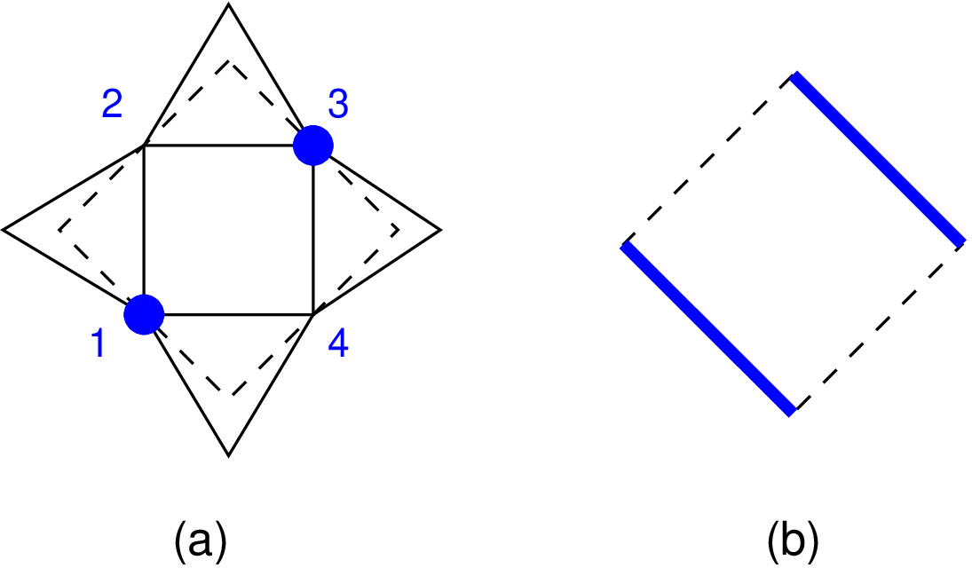
In what follows we present a complementary picture for the nature of the excitations above the plateau phase. This picture reveals the central role of the topology and the intrinsic spin and will emerge from the derivation of an effective quantum dimer model (QDM) in the spirit of Refs. Cabra; Bergman1; Bergman2 . The main idea is to start from the degenerate ground state configurations of the Ising limit and establish an adiabatic connection to the low-lying excitations of the Heisenberg point by employing a perturbative expansion in the anisotropy parameter . The resulting effective Hamiltonian can be cast into the form of a QDM on the dual clusters as exemplified in Figs. 8 and 9 for the cuboctahedron and the icosidodecahedron respectively. For a general spin , the ground state manifold of the Ising Hamiltonian spans all configurations with two spins having and one with in each triangle. Each one of these “uud” states on the cuboctahedron and the icosidodecahedron is in one-to-one correspondence to a closed-packed dimer covering on their dual clusters, the cube and the dodecahedron respectively.
III.2.1 Cuboctahedron
We start with the “uud” GS’s of the Ising cuboctahedron. There are nine such states since this is the number of different dimer coverings on the cube. This manifold, henceforth , decomposes into two invariant (under ) “uud” families and with 6 and 3 states respectively:
| (5) |
where
| (6) |
Each of the two families contains states with a fixed number (2 and 4 respectively) of square plaquettes of the type of Fig. 11(c) (this number remains invariant under the operations of the cluster).


The 9 “uud” states are highlighted in Fig. 10 which shows our symmetry-resolved ED results for , , and (at their sector) as a function of the anisotropy parameter . The energies are given in units of and for and respectively, which are the leading orders of the energy splitting due to (see below). Figure 10 shows that the Heisenberg states which are adiabatically connected to the lowest Ising manifold are not the lowest excitations for while this is clearly the case for higher spins and, as we show below, for the icosidodecahedron as well.
We shall try now to understand some of the features of Fig. 10 in more detail by considering the lowest order effect of in splitting the Ising nine-fold degenerate manifold, as a function of spin and . We follow the general guidelines and considerations of the Appendix A. We distinguish between diagonal and off-diagonal processes depending on whether the initial state is finally recovered or not. The former come from the smallest closed paths on the molecule (beyond triangles), which in the present case are the square loops (see left panel of Fig. 1) and the corresponding amplitudes scale with the fourth power of for all . Now, there are only three possible configurations on a square which respect the “uud” constraint and these are depicted in Fig. 11(a), (b) and (c). Each one carries a certain diagonal energy, say , and . We have calculated these energies as a function of using Eq. (23) and by enumerating all relevant processes. The results are
| (7) |
The Kronecker symbol appears in because some of the diagonal processes relevant for are not present for since they involve intermediate states which do not belong to the Ising manifold.33 3 This particular point for has been overlooked in Ref. Bergman2 in the context of the checkerboard lattice. Now, to any given Ising configuration there corresponds an associated potential energy equal to , where , , are the number of squares in the states , and , respectively in . On the other hand, we must satisfy two global conditions, one for the total number of squares , and another for the total number of down spins . This leaves us with one independent, non-global variable, say , in terms of which one can express . Omitting a global energy term , we find with
| (8) |
which is positive for and negative otherwise. The corresponding (lowest order) effective diagonal Hamiltonian reads
| (9) |
where the sum runs over all six square plaquettes (with both orientations) of the cluster. We may easily check that among all nine possible dimer coverings of the cube, three of them have and thus , while the remaining six have and thus . These correspond to the two families of “uud” states mentioned above, see Eq. (5). Hence, the eigenvalues of form a pair of a 6-fold and a 3-fold degenerate levels with an energy splitting of between them. In particular, this splitting amounts to for and for .

We now consider off-diagonal processes. To lowest order in , these are confined to the maximally flippable even-length loops of the cluster. These loops are the alternating spin up-down configurations already shown in Fig. 8. The corresponding flipping amplitude scales as . Their explicit values for several are provided in Table 7 (with ) of Appendix A. Thus the leading kinetic effect is described in the dimer representation by the term
| (10) |
where can be calculated explicitly using Eq. (23) and enumerating all different processes. Several representative values are provided in Table 7. The eigenvalues of in units of are: . These correspond to a complete splitting of the different IR’s of each of the two families of Eq. (5).
According to the above, our effective quantum dimer model should generally include both kinetic and potential terms. To leading order, this model reads
| (11) |
For we have , and the dynamics is mainly governed by kinetic processes which split completely (cf. Fig. 10(a)) the nine “uud” states. For we have , and thus both diagonal and off-diagonal processes are equally important. For the diagonal processes dominate and give rise to a splitting of between and of Eq. (5). In particular, since , the states of will be favored because they have a larger number (four) of the plaquettes of Fig. 8(c). All these features are nicely demonstrated in Fig. 10 where we compare our ED results for the XXZ model at small with the leading order eigenvalues of Eq. (11) which are shown as (red) filled squares.
III.2.2 Icosidodecahedron
We turn now to the corresponding plateau phase of the Heisenberg icosidodecahedron and follow a similar analysis as above. Here the lowest Ising manifold, henceforth , consists of 36 “uud” states which are in one-to-one correspondence with the 36 dimer coverings of the dodecahedron. We find that this manifold decomposes into two invariant (under ) families and of 30 and 6 states respectively as
| (12) |
where
| (13) |
Each of these families contains states with a fixed number (8 and 10 respectively) of pentagonal plaquettes of the type of Fig. 12(c) (this number remains invariant under the symmetry operations of the cluster). We should note in particular that each of the 6 states of contain two pentagons with all spins pointing up (i.e. have , cf.Fig. 12(a)).
A simple inspection of Fig. 13(a), which shows the lowest energy spectrum of the XXZ model, reveals that the lowest 36 Heisenberg states trace back to the ground state “uud” manifold of the Ising point. A striking difference to the cuboctahedron case studied above is that as these lowest Ising states “evolve” toward their low-lying Heisenberg counterparts, they remain always well separated from the higher energy states in the subspace. We now give a complementary picture, which is valid at least for small , by considering the lowest order processes driven by and by deriving the corresponding effective QDM on the dodecahedron. We begin with the lowest order off-diagonal processes. As above, these stem from maximally flippable loop configurations of the smallest possible even length . Such a loop configuration that respects the local “uud” constraint is the octagonal loop with alternating up-down spins depicted in Fig. 9(a) which in turn maps to the flippable plaquette of the dodecahedron shown in Fig. 9(b). For spin then, the lowest off-diagonal term in is of fourth order in . Each “up-down” loop of the type shown in Fig. 9(a) is amenable to a kinetic process of the form . From our calculations, shown in Table 7, we obtain . In fifth order, we find two types of kinetic processes. The first is similar to the above but now involves loops of length such as the equators of the molecule. The second type is less obvious, and invokes again the octagonal loops of Fig. 9(a) and any one of the neighboring spin sites. Since these loops map to exactly the same flippable dimer plaquette of Fig. 9(b) their effect is to merely renormalize the fourth-order amplitude . In fact, these terms result in an overall decrease of since they carry an extra negative sign.

On the other hand, the lowest order diagonal processes must be confined to the smallest closed path which in the present case are the pentagons of the molecule (see right panel of Fig. 1). The three possible types of configurations that respect the “uud” constraint around a pentagon are depicted in Fig. 12 and are designated by , and . Each one carries a certain diagonal energy, say , and . These are calculated by enumerating all relevant processes and using Eq. (23) of Appendix A. They are explicitly given by
| (14) |
To any given Ising configuration there corresponds an associated energy equal to , where , , are the number of pentagons in the states , and respectively in . On the other hand, we must again satisfy two global conditions, one for the total number of pentagons , and one for the total number of down spins . This leaves us with one independent, non-global variable, which we choose to be . Omitting a global energy , we find , with
| (15) |
which is positive for all . This means that favors configurations with the minimum number of the pentagonal states of Fig. 12(c). Since all 30 states of have while the 6 states of have , the former family will be lower in energy by a splitting of . Furthermore, it is clear that diagonal processes do not give rise to a splitting within the two families.


| Energy | deg. | Energy | deg. |
|---|---|---|---|
| -4 | 1 | -0.694593 | 5 |
| -3.06418 | 5 | 1 | 4 |
| -2.89898 | 1 | 2 | 5 |
| -2 | 5 | 3.75877 | 5 |
| -1 | 4 | 6.89898 | 1 |
case.— Given all the above, the effective QDM for the plateau phase of the Heisenberg icosidodecahedron is, at lowest order, dominated by kinetic, off-diagonal processes of the form
| (16) |
where the sum runs over all octagonal plaquettes and . The corresponding Hamiltonian matrix can be constructed and solved numerically for its eigenvalues. These are provided in Table 4 in units of . They are also shown as filled squares in Fig. 13(b). In the same figure, we show the lowest 36 eigenvalues (divided by ) of in units of . The clear convergence for small toward the eigenvalues of confirms the validity of our perturbative calculations. Moreover, the fact that the convergence is linear confirms that the next processes contributing to come in fifth order. In particular, the clear decrease of the bandwidth with is in agreement with our previous assertion that the fourth order amplitude of Eq. (16) gets renormalized from the fifth order octagonal kinetic processes mentioned above. The latter seem to dominate over the corresponding fifth order off-diagonal decagonal loop processes and the fifth order diagonal ones. Looking at Fig. 13(a) one notes that this may be even more general: To all orders in , there seems to be a mere renormalization of the bandwidth without drastically altering the relative amplitudes of the eigenvalues of . This suggests a dominance of the most local (octagonal) kinetic processes renormalized from all orders in .
and relevance to Mo72Fe30.— As mentioned above, diagonal processes first appear in fifth order irrespective of . On the other hand, the lowest off-diagonal process on a loop of (even) sites appears in order . For instance, the octagonal loops discussed above give processes at order (and higher), whereas decagonal (e.g. the equatorial) loops contribute in order (and higher). Hence for diagonal and off-diagonal processes are equally important, while for the physics will be completely dominated by diagonal processes of fifth order in :
| (17) |
where the sum runs over all pentagonal plaquettes (with all possible orientations) and is given by Eq. (15). As explained above these processes result in a diagonal splitting of between and with the former family being lowest in energy. For in particular, which is relevant for the plateau phase of Mo72Fe30 Fe30_Plateau, this splitting amount to the quite small value of . Since, at the same time, the excitations out of the Ising manifold are expected to remain gapped for the finite value of , we speculate that the plateau phase of Mo72Fe30 must show a characteristic low-temperature thermodynamic signal which is qualitatively similar to that of Fig. 7 (up to fine details related to the 30 to 6 diagonal splitting). Here, in particular, the entropy content of the renormalized “uud” manifold amounts to approximately of the full magnetic entropy. This calls for low-temperature specific heat measurements on Mo72Fe30 at the plateau phase as explained in Sec. III.1. More generally, it is exciting that the notion of a Quantum Dimer Model finds a realization in the low-energy plateau physics of finite-size magnetic clusters like Mo72Fe30 or Mo72V30.
IV Heisenberg spectra for
The major focus of this section is on Heisenberg spectra with . Our interest in this regard is mainly motivated by the INS experiments reported by Garlea et al. Garlea_INS on Mo72Fe30. The main finding of these experiments is a very broad response which manifests in a wide range of fields. Previous theories which are based either on the excitations of the rotational band model Garlea_INS; SchnackLubanModler or on spin wave calculations Cepas_LSW; Waldmann_LSW, could not account for the observed behavior since they predict only a small number of discrete excitation lines at low temperatures. Although the diagonalization of the icosidodecahedron is not feasible (at low magnetizations) with current computational power, an immediate interpretation of this behavior can be deduced from a study of the cuboctahedron. Exact diagonalization spectra of this cluster for and are shown in the two lower panels of Fig. 14. For comparison we have also included the spectrum (this was shown before in the middle panel of Fig. 4 in terms of instead of the total spin ). Here, in contrast to unfrustrated clusters (cf. upper panel of Fig. 4), there does not exist any well isolated and thus clearly identified low-energy tower of states or rotational band. Instead, a “bulk” of very dense excitations are present in the full magnetization range. This is a generic feature of highly frustrated systems which manifests irrespective of and thus must be also present in the Mo72Fe30 cluster (similarly to its analogue of Fig. 4).
The origin of these dense excitations for can be readily suggested by the following striking observation in Fig. 14: The spectra consist, up to a relatively large energy cut-off, entirely of the representations A1g, A2g, Eg, and T2u. The main message in the following is that this peculiar spatial symmetry pattern as well as the combined spatialspin pattern (i.e., the appearance of specific sets of spatial IR’s in each sector) are characteristic fingerprints of the 3-sublattice Heisenberg classical GS’s. For instance, as we explain below, these four representations are exactly the ones that appear in the symmetry decomposition of the coplanar classical GS’s (cf. Eq. (IV.1) below). The dense excitation features of the lower two panels of Fig. 14 can be thereby accounted for by the large spatial degeneracy of these configurations, a fact whose importance does not seem to have been recognized in the past. In principle, each of these states gives rise to a distinct “tower of states” or “rotational band” and they all appear together at low energies albeit split by quantum fluctuations. So the large discrete degeneracy has a direct impact on the low-energy spectrum, and we believe this large number of levels is at the very heart of the broad INS response reported in Ref. Garlea_INS. By contrast, the absence of a clear symmetry pattern in the spectra (cf. upper panel of Fig. 14) shows that the associated low-lying excitations are of different origin.


Before analyzing further our numerical results it is useful to recall (cf. Subsec. IV.1 below) what is known about the classical GS’s of the infinite kagomé lattice in zero and finite field and discuss what carries over in the present clusters. In particular, we give the explicit spatial degeneracy of the coplanar GS’s and a short summary of their symmetry properties. The latter have been derived independently by employing a group theoretical analysis, the details of which have been relegated to Appendix B. Our semiclassical interpretation for the origin of the dense excitations of the above spectra will be further corroborated by a closer comparison of the symmetry pattern of the spectra with the combined spatialspin symmetry of the coplanar GS’s also derived in Appendix B. In Subsec. IV.2 we discuss the simpler case of the XY model which exemplifies very evidently the main idea of this section, i.e., the simultaneous presence of several lowest towers of states due to the discrete classical degeneracy.

IV.1 Classical GS’s and large spatial degeneracy
Let us first consider the ground state configurations of the classical Heisenberg model in the infinite kagomé system and the present clusters. The corner-sharing triangles structure makes the discussion rather simple. The classical Hamiltonian can be rewritten in the suggestive form (in units of )
| (18) |
where denotes the total spin on a triangle . In this form it is straightforward to see that all configurations with on each triangle are GS’s. It is useful to examine the zero-field case first.
Zero-field case.— Here, the classical constraint amounts to a simple 120∘ configuration of the three spins, which is depicted in Fig. 15(a). An important point here and in the following is to determine how many such GS’s exist. For the kagomé lattice it is well known that the ground state manifold consists of both coplanar and non-coplanar configurations in zero field. The coplanar GS’s are extensively degenerate as can be shown by a mapping onto vertex three-colorings of the kagomé lattice or equivalently onto bond three-colorings of the Honeycomb lattice Potts; BaxterThreeColorings. On the other hand the non-coplanar GS’s can be generated from the coplanar ones by the following recipe: Identify a loop of alternating spin orientations (two out of three directions), which is either closed or extends to infinity. All sites neighboring the loop share the common third spin direction. It is then possible to collectively rotate the spins on the loop freely around the third direction at zero energy cost. Such a new state is clearly non-coplanar, but still a ground state.

Let us now discuss what carries over of this large classical degeneracy on the two present molecules. It is straightforward to enumerate all vertex-three colorings for both the cuboctahedron and the icosidodecahedron and the respective numbers are 24 and 60, or 4 and 10 if one discards global recolorings. Two such states of the cuboctahedron are illustrated in Fig. 16, while a typical one for the icosidodecahedron can be found in Fig. 2 of Ref. AxenovichLuban. We stress here that these 4 and 10 states are unrelated by the global symmetry, and therefore form genuinely different GS’s and give rise to distinct “tower of states” at low-energies. The spatial symmetry properties of these states have been derived in Appendix B and can be summarized as follows. The 24 vertex three-colorings of the cuboctahedron form two invariant (under the operations of ) families and which consist of 6 and 18 states respectively, and they decompose into IR’s of as
| (19) |
As mentioned above, these are exactly the IR’s that appear (with open symbols) in the spectra of the lower two panels of Fig. 14. On the other hand, the 60 vertex three-colorings of the icosidodecahedron form two invariant (under the operations of ) families which are equivalent to each other (cf. Appendix B). Here, we shall treat these families collectively as a single one called . This decomposes into IR’s of as 44 4 We should note here that larger clusters have a larger number of coplanar GS’s and thus decompose into an accordingly larger number of spatial IR’s (eventually containing all possible spatial IR’s for large enough sizes). This can be already seen for the icosidodecahedron whose classical GS’s decompose into 8 out the 10 different IR’s of . The cuboctahedron on the other hand, has a small number of coplanar GS’s and this allows to recognize their traces in the low-lying excitation spectra.
| (20) |
As to the non-coplanar GS’s (in zero-field), it turns out that the icosidodecahedron has none, since all the alternating loops described above have maximal length (20), and therefore the rotation of the spins on the loop just changes the global spin plane, thus preserving the coplanarity. The cuboctahedron however has non-coplanar GS’s, since the loops can have length shorter than eight, in agreement with previous studies AxenovichLuban; SchmidtLuban.
When switching on quantum fluctuations on the kagomé lattice it is known that the spin waves at harmonic order select the coplanar GS’s over the non-coplanar ones (order-by-disorder effect), due to the larger number of soft modes of the former HarrisKallinBerlinsky. A complete lifting of the remaining (spatial) degeneracy is taking place at the level of anharmonic spin waves, whereby the single magnetically ordered state is selected Chubukov; ChanHenley. On the other hand for the extreme quantum case of a number of numerical works clearly show the absence of any magnetic order Lecheminant_kagome; Waldtmann. So based on these conflicting results it is difficult to predict to which regime the intermediate values of spin will belong.
| Cuboc. | Cuboc. | Icosi. | ||||
| N | N | N | ||||
| 0 | A1g | 1 | A1g,Eg | 3 | Ag,Au,Fg,Fu | 10 |
| 1 | A2g,Eg | A1g,Eg, | Ag,Au,Fg,Fu, | |||
| 3 | 2T2u | 9 | 2(Hg,Hu) | 30 | ||
| 2 | A1g,2Eg | 3(A1g,Eg), | Ag,Au,Fg,Fu, | |||
| 5 | 2T2u | 15 | 4(Hg,Hu) | 50 | ||
| 3 | A1g,2A2g,2Eg | 3(A1g,Eg), | 3(Ag,Au,Fg,Fu), | |||
| 7 | 4T2u | 21 | 4(Hg,Hu) | 70 | ||
| 4 | 2A1g,A2g,3Eg | 5(A1g,Eg), | 3(Ag,Au,Fg,Fu), | |||
| 9 | 4T2u | 27 | 6(Hg,Hu) | 90 | ||
| 5 | A1g,2A2g,4Eg | 5(A1g,Eg), | 3(Ag,Au,Fg,Fu), | |||
| 11 | 6T2u | 33 | 8(Hg,Hu) | 110 | ||
| 6 | 3A1g,2A2g,4Eg | 7(A1g,Eg), | 5(Ag,Au,Fg,Fu), | |||
| 13 | 6T2u | 39 | 8(Hg,Hu) | 130 |
We now give a symmetry analysis for the cuboctahedron spectra at low magnetizations which suggests strongly that the low-lying excitations can be described in semiclassical terms at the harmonic spin-wave level. To this end, we should first emphasize that the non-coplanar GS’s do not carry the above spatial symmetry because not all triangles share the same spin plane in these configurations and thus spatial operations generally cannot relate different triangles. This means that the striking agreement between the spatial symmetry of the above low-energy spectra and Eq. (IV.1) is not just accidental. Of course there can be other states whose spatial decomposition can in principle contain some or all of the IR’s of Eq. (IV.1) (in fact such states will be examined below for finite magnetizations). More stringent evidence comes by comparing the full spatialspin symmetry pattern of the exact spectra to that of the 120∘ states. The latter has been derived in Appendix B and the results are provided in Table 5 up to . A closer inspection of the and spectra (cf. lower two panels of Fig. 14) shows a remarkable agreement: All lowest-energy levels (shown with open (black) symbols) which are below the levels shown with filled (red) symbols can be identified in Table 5 with the right combinations of spatial and spin representations and multiplicity. It is important to note here that, although these towers are severely split by quantum fluctuations —in fact some IR’s of Table 5 (e.g. one A1g level at the sector) can be found slightly higher than the lowest (red) filled symbols— almost the entire set of levels contained in Table 5 are found below the filled symbols with no extra level appearing. Thus we believe the combined spatialspin symmetry pattern of the spectra for small magnetizations is a characteristic fingerprint of the 120∘ semiclassical states.
Finite-field case.— Here the ground state manifold is generally larger since the classical constraint allows for non-coplanar configurations already at the level of a single triangle. It is known Shender; ZhitoPRL02; Hassan however that the coplanar states with the spins lying in the field-plane have the largest number of soft modes and thus must be selected by quantum or thermal fluctuations. A subsequent selection which depends on the field takes place within the field-plane for the orientation of the spin triad ZhitoPRL02. It turns out that the most relevant GS’s in a finite field are the ones depicted in Figs. 15(b) and (c). 55 5 Note that the remaining degeneracy is lifted already by harmonic spin waves Hassan with a selection of the state at small fields and a peculiar competition between the and the state at higher fields (cf. Fig. 8 of Ref. Hassan). For (cf. Fig. 15(b)) the relevant GS’s on a triangle form a one-parameter family with one spin anti-parallel to the field. It is important to note that, apart from their difference in the directions of the three spins, these configurations are spatially indistinguishable from the 120∘ states of Fig. 15(a): They are both 3-sublattice states and thus carry the same spatial multiplicity (i.e. 24 for the cuboctahedron and 60 for the icosidodecahedron) and the same spatial symmetry (i.e., Eqs. (IV.1) and (20)). Quite similarly, the “quasi-collinear” configurations of Fig. 15(c), which can be selected for , have an “uud” spatial structure. Hence they share the same spatial multiplicity and symmetry properties with the Ising GS’s. Namely, there exist and “quasi-collinear” states for the cuboctahedron and the icosidodecahedron respectively, and their spatial symmetry is given already in Eqs. (5) and (12). We should note here that the set of IR’s appearing in Eqs. (5) and (12) form a subset of the ones appearing in Eqs. (IV.1) and (20) respectively. 66 6 An explanation of this feature can be readily given for the cuboctahedron: Here the 9 “uud” colorings can arise from the 24 vertex three-colorings by identifying e.g. A with B and thus the symmetry IR’s of the former are contained in the latter. Things are slightly different for the icosidodecahedron: Here the 60 vertex three-colorings of provide (by identifying A with B) only the 30 “uud” colorings of . Each of the remaining 6 “uud” states of contain two pentagonal loops of the type of Fig. 12(a) (i.e. they have ) with five spins pointing up and thus cannot arise from a vertex three-coloring (since we cannot put alternating A, B spins on a pentagon).
According to the above, all types of semiclassical configurations of Fig. 15 have the same set of spatial representations, except the “quasi-collinear” states which do not contain the A2g representation: At large magnetizations this level is pushed higher in energy and this seems to confirm that it does not belong to the relevant towers of states of the “quasi-collinear” classical states. More generally, the fact that the same set of spatial IR’s appear in the low-energy spectra at all magnetizations signifies that our previous semiclassical interpretation for the zero-field case carries over for finite fields as well. Again, one may ask for more stringent evidence by a comparison of the combined spatialspin symmetry properties of these finite-magnetization states. We have derived these combined symmetries (not shown here) following the same lines as in Appendix B, but it turns out that the small size of the cuboctahedron together with the severe splitting of the low-lying states do not allow for a straightforward and thus definite identification of the relevant towers of states as above. As we show below, this will be possible for the much simpler case of the XY model.
IV.2 XY model
Here we study the XY model (i.e. the limit of Eqs. (2)-(4)) on the cuboctahedron. The reason of doing this is twofold. First because, in contrast to the Heisenberg point, the XY point exemplifies very evidently the core idea of the simultaneous appearance of several towers of states due to the spatial degeneracy of the classical GS’s. And second, to provide an additional interpretation of the Heisenberg spectra, since these can be thought of as being adiabatically connected to the XY spectra but split by the quantum fluctuations introduced by .


We first consider the classical case with a magnetic field perpendicular to the -plane. As above, the XY Hamiltonian can be rewritten in terms of the three spins of each triangle and its total spin as (in units of ):
| (21) |
where and similarly for . The leading term of Eq. (21) is minimized by taking on each triangle. The remaining terms require that we maximize both and with the constraint (the balance between the two components is controlled by the ratio ). In zero-field this gives the 3-sublattice states where all triangles share the same spin (xy) plane. The major difference with our previous analysis of the Heisenberg (classical) GS’s is that here a spin plane (i.e. the plane) is selected explicitly from the beginning (i.e., for zero field) and this gives a finite energy cost to non-coplanar configurations. A finite field gives rise to a tilt of the three spins out of the xy plane giving rise to the so-called “umbrella” states. It is clear that both in zero and in finite field, the classical XY GS’s have the same spatial multiplicity and spatial symmetry properties (but not spin symmetry properties, see below) with the set of coplanar 3-sublattice GS’s of the Heisenberg point.
| Cuboc. | Cuboc. | Icosi. | ||||
|---|---|---|---|---|---|---|
| N | N | N | ||||
| A1g | 1 | A1g,Eg | 3 | Ag,Au,Fg,Fu | 10 | |
| A2g | 1 | T2u | 3 | Ag,Au,Fg,Fu | 10 | |
| Eg | 2 | A1g,Eg,T2u | 6 | 2Hg,2Hu | 20 | |
| A1g,A2g | 2 | A1g,Eg,T2u | 6 | 2(Ag,Au,Fg,Fu) | 20 |
Let us now consider the quantum-mechanical XY model. For our demonstration purposes, it suffices to consider the case only (the case is very similar77 7 Interestingly the XY model spectrum (not shown here) resembles much more the Heisenberg spectra of Fig. 14, and does not show the well separated tower of states of the large XY model.). The low-energy spectrum is shown in the upper panel of Fig. 17. A number of spectral features are revealed. First, in contrast to the Heisenberg case studied above, the lowest-energy portion of the spectrum (indicated by the arrow) is well isolated from higher excitations and it comprises four distinct towers of states. This multiplicity is a fingerprint of the spatial degeneracy of the classical 3-sublattice states mentioned above. This can be further substantiated by examining more closely the symmetry structure of the excitations intervening in these towers. To this end we zoom in on these towers in the lower panel of Fig. 17. A simple inspection of the spatial IR’s that appear in this panel reveals that they are exactly the ones given by Eq. (IV.1). Much stronger evidence comes by examining the full spatialspin symmetry structure of the lowest towers. Indeed, a closer comparison to Table 6 (derived in Appendix B) demonstrates that there is a remarkable one-to-one correspondence of each of the lowest towers with the classical families which holds in almost the entire magnetization range. We should emphasize here that each semiclassical state shows a different and quite non-trivial symmetry pattern which is in some sense a very characteristic fingerprint of the state. For instance, the full content of 24 states of Eq. (IV.1) is recovered every three sectors in the lowest towers with the specific pattern of combined spatial and spin IR’s given in Table 6. This remarkable agreement between exact ED spectra and our symmetry derivation is indeed a strong evidence that the lowest towers of states can be thought of as renormalized semiclassical 3-sublattice states.
Some additional remarks are in order here regarding the energies of the two families of towers as revealed in the lower panel of Fig. 17. We should first note that all towers are expected to become degenerate in the classical limit. Based on spectra with (not shown here), we find that the energy splittings within a tower of each of the two families and diminishes quickly on increasing as expected, while at the same time, the energy splitting between them remains sizable. On the other hand, as a function of (or field), there is an interesting level crossing between the two families somewhat below the magnetization plateau, with the family being more favorable below this point. An understanding of the above level-crossing could arise by employing for instance a semiclassical expansion for the XY model in a field, in a similar fashion with what is done for the Heisenberg model Henley; Hassan, but such an analysis is clearly beyond the scope of this paper.
V Summary
We have presented an extended study of the low-energy physics of two existing magnetic molecule realizations of the kagomé AFM on the sphere, the cuboctahedron and the icosidodecahedron. Our ED results revealed a number of generic spectral features which stem from the corner-sharing topology of these clusters. Indeed, a simple comparison to a finite-size unfrustrated magnet demonstrated that frustrated clusters manifest a “bulk” of very dense low-energy excitations. We focused on two major aspects which are of general interest but were particularly oriented toward the Mo72Fe30 cluster: (i) the low-energy excitations above the plateau and (ii) the low-lying spectra of the Heisenberg model for .
For the plateau, we first demonstrated that the icosidodecahedron shows 36 low-lying excitations which are adiabatically connected to collinear “uud” Ising (GS’s), at the same time being well isolated from higher levels by a relatively large energy gap. We then argued, based on a complementary physical picture which emerged from the derivation of an effective quantum dimer model, that this feature must be special to the topology of the icosidodecahedron and that it must survive for as well. We also predicted that the corresponding 36 low-lying plateau states of the icosidodecahedron consist of two “uud” families (of 30 and 6 states respectively) which are separated by a small diagonal energy splitting. This result can be confirmed by low-temperature specific heat measurements at the regime ( Tesla) of Mo72Fe30 and/or by an assessment of the associated missing entropy.
In the second part, we showed exact diagonalization spectra for the Heisenberg cuboctahedron which demonstrated that the dense low-lying excitation features of the case are present for as well, albeit with a striking spatialspin symmetry pattern. These spectra provide a semiclassical interpretation of the broad inelastic neutron scattering response reported for Mo72Fe30. The main ingredient of this interpretation is the simultaneous presence of several low-energy towers of states or rotational bands at low energies which originate from the large spatial multiplicity of the classical Heisenberg ground states, and this is known to be a generic feature of highly frustrated clusters. This semiclassical interpretation was further corroborated by an independent group theoretical analysis which demonstrated that the striking symmetry pattern of the low-lying excitations is indeed a characteristic fingerprint of the classical coplanar ground states. The core idea of the simultaneous presence of several rotational bands at low energies due to the discrete classical degeneracy was finally exemplified very evidently by a study of the XY model.
VI Acknowledgments
We would like to acknowledge fruitful discussions with C. L. Henley, M. Luban, and K. P. Schmidt and earlier collaboration with J.-B. Fouet and S. Dommange on related subjects. The point group symmetry data used in our calculations have been obtained using the Bethe package Bethe. We would like to thank K. Rykhlinskaia for her assistance with this package. This work was supported by the Swiss National Fund and by MaNEP. The computations have been enabled by the allocation of computational resources on the machines of the CSCS in Manno.
Appendix A Degenerate Perturbation Theory around the Ising point
Here we describe some very general considerations which greatly facilitate the classification of processes appearing in degenerate perturbation theory around the Ising point. We consider corner sharing triangles structures with general spin , and focus on the plateau. The ground-state Ising manifold consists of configurations which maximize the number of extremum local moments Bergman1. At the plateau phase, this consists of all configurations with two spins having and one with in each triangle. All processes triggered by must preserve this constraint. Let us denote by the zero-th order energy and by the projections onto and out of the Ising manifold. We also designate by the resolvent operator
| (22) |
The -th order term of the effective Hamiltonian in the Rayleigh-Schrödinger formulationDPT reads
| (23) |
where each of the “remaining terms” can be thought of as a product combination of lower order terms (with ). This separation is useful when e.g. all processes below some order are constant since then, to order , it suffices to keep only the leading term of Eq. (23). The presence of ’s in Eq. (23) enforces all terms to flip spins in such a way as to respect the “uud” constraint in each triangular unit.
The derivation of at any given order is greatly facilitated by noting that only “linked” processes should be taken into account. These are interactions that are “connected” in the following sense. Substituting in Eq. (23) gives different types of terms, each one carrying a string of a given number of bond operators . We differentiate between “linked” and “unlinked” interaction terms depending on whether the set of all vertices appearing in the corresponding string forms a connected (open or closed) path in the lattice or not. The latter contain nonlocal interactions between disconnected parts of the lattice and therefore must be omitted DPT. Only connected paths should therefore be considered. Further simplifications arise from the “uud” constraint as described below for diagonal and off-diagonal processes.

Diagonal processes.— As explained in considerable detail in Ref. Bergman1 in the context of the pyrochlore lattice, all diagonal processes up to a given order give an overall constant energy shift, with the leading non constant terms arising from processes along closed loop configurations. As we explain below, similar results apply to the present case of corner sharing triangles as well. The proof can be demonstrated in a compact way by using the contraction method of Bergman et al. Bergman1
Consider first all-order diagonal processes confined to a given triangle. Clearly, the only physically distinct configuration on this triangle is the “uud” one, since the associated diagonal energy does not depend on which of the three vertices the down spin resides (cf. Fig. 18(a)). By sampling the energies of all triangles we end up with an energy that is global, i.e., the same for all Ising states. Hence all-order processes confined in a single triangle give an overall constant energy shift and can thus be neglected. We now consider all-order processes confined to two adjacent triangles. Here, there are two physically distinct classes of configurations (cf. Fig. 18(b)), depending on whether the shared spin points down (first state in Fig. 18(b)) or up (remaining four states). Since all four states with the shared spin pointing up are physically equivalent, the energy is only a function of the shared spin variable. By sampling again over the lattice we obtain a global energy shift. Remarkably, these arguments can be generalized to much broader cases by the contraction method exemplified in Fig. 18(c): Since permuting the spin variables 2 and 3 results in a topologically equivalent state, knowing the value of is enough, i.e.,
| (24) |
where designates all remaining spin variables. This “contraction” can be continued with the next available triangle inside the shaded area , and so on. If this process can be continued until we are left with a function of a single vertex, then sampling this function over all spins we obtain again a global energy shift.

A non-constant energy contribution may arise only when the contraction process cannot be continued until the last spin variable. This happens whenever the shaded area of Fig. 18(c) contains one or more closed loops, since none of the triangles making up a loop is “contractible”. This leaves us with the following quite general statement: All-order processes confined to a fragment of the lattice with no closed loops give an overall constant energy shift. The most general form of such fragments is depicted in Fig. 19 and is recognized to be a Bethe lattice made of triangles, known as Husimi cactus.
Hence, the lowest order diagonal processes come from closed loops in the lattice. One should also remark that, in contrast to off-diagonal processes (see below), the order at which diagonal processes first appear is independent of the spin .

| L | 2s | Order () | # of processes | |
|---|---|---|---|---|
| 4 | 1 | 2 | -1.0 | 4 |
| 2 | 4 | -1.0 | 36 | |
| 3 | 6 | -0.5625 | 400 | |
| 4 | 8 | -0.25 | 4 900 | |
| 5 | 10 | -0.09765625 | 63 504 | |
| 6 | 12 | -0.03515625 | 853 776 | |
| 6 | 1 | 3 | 1.5 | 12 |
| 2 | 6 | -0.88402469 | 900 | |
| 3 | 9 | 0.25093125 | 94 080 | |
| 4 | 12 | -0.05637473 | 11 988 900 | |
| 5 | 15 | 0.01106939 | 1 704 214 512 | |
| 6 | 18 | -0.00199964 | 260 453 217 024 | |
| 8 | 1 | 4 | -2.5 | 48 |
| 2 | 8 | -0.93709194 | 45 360 | |
| 3 | 12 | -0.12770306 | 60 614 400 | |
| 4 | 16 | -0.01464521 | 114 144 030 000 | |
| 10 | 1 | 5 | +4.375 | 240 |
| 2 | 10 | -1.0924858 | 3 855 600 |
Off-diagonal processes.— Figure 20 shows schematically a given lattice path (solid thick line) with two particular configuration choices. All spins have except the ones indicated by filled circles with . By definition, only spins residing on this path may be flipped. In off-diagonal processes at least one spin, say , is flipped from to . But, since the final state must preserve the “uud” constraint in each triangle, flipping must be accommodated by a similar flip of the adjacent spins lying on the path, namely and . Similarly, the spins at vertices 2 and 3 must also be flipped. If, as drawn in Fig. 20(a), the initial configuration has , then flipping already violates the “uud” constraint. It is also clear that if the path is open at one end (or at both ends) the ending spin (or spins) will be flipped at the final state, thus violating the “uud” constraint on the adjacent triangle(s). Thus only closed, connected paths with alternating up-down spins, such as in Fig. 20(b) are amenable to an off-diagonal process. The simplest possible paths are loops of even number of spins . Since flipping each spin requires operations, off-diagonal processes on a simple loop appear in order . An example was shown in Fig. 9 for the icosidodecahedron. In Table 7 we provide calculated numerical values for the amplitude of such virtual processes around loops with , , and sites and various values of . Starting from a given loop, one may also build processes (and paths) of higher order by invoking adjacent triangular units. An example for the icosidodecahedron was the fifth order processes mentioned in Sec. III.2.2.
Appendix B Symmetry properties of the 3-sublattice coplanar states
Here we give the details of the derivation of the symmetry properties of the semiclassical 3-sublattice coplanar states of Fig. 15(a). These are relevant for the Heisenberg model at as well as the XY model (discussed in Sec. IV.2) for both zero and finite fields. As explained above, the spatial symmetry properties of the states of Fig. 15(b) are the same as that of (a), and similarly the spatial symmetry of the “quasi-collinear” states of Fig. 15(c) is identical to that of the “uud” states given in Eqs. (5) and (12). The derivation of the combined spatialspin properties of Fig. 15(b) and (c) are not of our interest here but can be found easily following the same steps as below.
We are using the following notation and conventions. The groups of real space and spin space operations are denoted respectively by and . In particular, for the cuboctahedron and for the icosidodecahedron. The full group is designated by . A stabilizer of a classical state consists of elements which preserve (i.e. ) and this will be either a subgroup of or a subgroup of depending on whether we are examining only the spatial or the full symmetry properties. The elements of , and are labeled by , , respectively, while their IR’s are denoted as , , and . Similarly, their characters are denoted by , , and . Let us first discuss the spatial symmetry and then the combined spatialspin symmetry structure of the 3-sublattice states.
B.1 Spatial symmetry of 3-sublattice states
As we discussed previously, each vertex three-coloring is in one-to-one correspondence with the states of Fig. 15(a). Starting from a given and applying all elements of we generate an invariant vector space or orbit . The decomposition of into IR’s of is given by the well known formula GroupTheory
| (25) | |||||
| (26) |
The matrix element is equal to one if belongs to the stabilizer of and vanishes otherwise. Thus we may rewrite Eq. (26) as
| (27) |
where we made use of . This relation follows from the coset decomposition of with respect to (each coset is in one-to-one correspondence with the states of the orbit ). Employing (27) to all different orbits we obtain the symmetry properties of the coplanar states.
Let us see now what happens for the cuboctahedron and the icosidodecahedron separately. As discussed above, the cuboctahedron has a total number of 24 vertex three-colorings . Under they form four invariant orbits of six colorings each. The first orbit, called consists of the six global permutations of the translationally invariant coloring depicted in Fig. 16(a). The 18 colorings that belong to the remaining three orbits result from the first orbit by interchanging colors along loops with two alternating colors. One such configuration is shown in Fig. 16(b). Although these three orbits are equivalent it is useful for the following discussion of the full spatialspin properties to treat them collectively as a single one which we term . 88 8 Our notation for these two orbits is borrowed from the corresponding points of the Brillouin zone of the 12-site kagomé, i.e. the point and the three -momenta at the middle points of the boundary edges. Note however that the three orbits of the M family are not in one-to-one correspondence with the three -momenta but rather combine all of them. The decomposition of the above orbits into IR’s of was given in Eq. (IV.1).
On the other hand the icosidodecahedron has 60 coloring states. Under they form two orbits of 30 colorings each. The first orbit consists of the 3 cyclic permutations (ABC,CAB,BCA) of 10 ABC states, while the second orbit consists of the remaining 3 permutations (or reflections) (BAC,CBA,ACB) of the same 10 states. Although these two orbits are equivalent it is useful for the discussion of the full spatialspin properties (see below) to treat them as a single one which we denote by . Its decomposition into IR’s of was given in Eq. (20).
B.2 Spatialspin symmetry of 3-sublattice states
We shall now go one step further and derive the combined spatialspin properties of the above states. Namely, a decomposition similar to that of Eqs. (IV.1) and (20) but now in terms of IR’s of the full symmetry group of the Hamiltonian. The method has been employed previously in the seminal works of Bernu et al. Bernu1; Bernu2 and Lecheminant et al. Lecheminant_J1J2; Lecheminant_kagome.
The recipe is quite analogous to the one we employed above. Here however, by applying the elements of the full group on a given classical state we generate a continuous orbit . All states contained in this orbit are coplanar but their order parameter has all possible orientations in spin space ( is a continuous “order parameter space”). Otherwise, the equation giving the numbers (i.e. how many times is appearing in the decomposition of into IR’s of ) is fully analogous to Eq. (27) and reads
| (28) |
where now . For the identification of it is expedient to split the operations of the space group into the sets defined as follows. The first consists of elements which map to itself. On the other hand, the elements of map to its globally permuted (ABC) (CAB) version, and similarly for the remaining sets. We also define the following set of integer numbers
| (29) |
These numbers depend on the transformation properties of under the spatial group alone. The non-vanishing ones are given in Table 9.
| 1 | 1 | 1 | |
| 1 | 1 | -1 | |
| 2 | 2 | 0 |
We should note here that one can make a choice of depending on the amount of information we seek. For instance we may choose according to the symmetries we implement in our exact diagonalizations. We may even take as the idenity, i.e. . In the latter case we recover Eq. (27). The type and number of invariant vector spaces in each case will be different and the symmetry decomposition must be applied to each one separately, but the corresponding results will be consistent with each other.
Let us now apply the above to the zero-field Heisenberg model and the XY model.
| Cuboc. | Cuboc. | Icosi. | |
|---|---|---|---|
| (A1g,A2g,Eg) | (A1g,Eg,T2u) | (Ag,Au,Fg,Fu,Hg,Hu) | |
| 48 | 16 | 12 | |
| (8, 8,16) | (8, 8, 8) | (4, 4, 4, 4, 8, 8) | |
| (8, 8,-8) | (4, 4, 4, 4,-4,-4) | ||
| (8, 8,-8) | (4, 4, 4, 4,-4,-4) | ||
| (8,-8, 0) | (8, 8,-8) | ||
| (8,-8, 0) | |||
| (8,-8, 0) |
B.2.1 point
Here we take and is the total spin which is integer here. A single generates the full set of coplanar states for each family of the clusters. The elements of , , and can be combined with rotations of and bring back to itself. Thus again . Using Eq. (28) with then
| (30) | |||||
where GroupTheory . Replacing the values of Table 9 for each family separately we obtain the symmetry structures given in Table 5.
B.2.2 XY point
Here, we take which includes rotations and the continuous set of vertical (i.e. containing the -axis) mirror planes. The IR’s of can be generally labeled GroupTheory by a non-negative integer or , with an additional label for which stands for the parity under the mirror operation. Hence . All IR’s for are two-dimensional and consist of pairs of and basis vectors. The characters of are given in Table 8.
It suffices to select a single coloring state since this generates all coloring states for both clusters. The stabilizer can be found as follows. Each one of the sets , , etc. discussed above can be combined with one of the elements of to give again. For instance, an element of can be combined with a spin rotation of . On the other hand, an element of can be combined with a mirror plane containing the -axis (i.e. that of the spins “colored” as ). The set of all such combined operations span , i.e. . Using Eq. (28) with then
| (31) | |||||
Replacing the values of Table 9 and the characters from Table 8 for each family separately we obtain the symmetry structures given in Table 6. According to this table, the symmetry pattern repeats itself every three sectors. In particular, the full set of spatial IR’s of Eqs. (IV.1) and (20) is contained in any triad of subsequent sectors. As can be seen from the above relations, this periodic pattern stems from the 120∘ 3-sublattice symmetry structure of the coplanar states (the character (with ) has a period of ).
In connection to a remark above, it is clear that we could have chosen here instead of . The corresponding stabilizer would then obviously be different from the above since none of the combinations of , and with rotations can bring to itself. Nevertheless, the results from the two different choices of are consistent with each other.
We should finally emphasize a non-trivial feature which appears in both Tables 6 and 5 and holds for each family separately. Namely that the total number of states (counting the degeneracy of spatial IR’s) for a given IR of the spin group is equal to the dimensionality of this IR (i.e. for the Heisenberg case, see Table 8 for the XY case) times the ratio . This feature can be proven by group theory alone using , Eq. (28) and the so-called character orthogonality relation GroupTheory.
References
- (1) G. Misquish and C. Lhuillier, in Frustrated Spin Systems, edited by H. T. Diep (World Scientific, Singapore, 2004), pp. 229-306.
- (2) J. Richter, J. Schulenburg, and A. Honecker, Lect. Notes Phys. 645, 85 (2004).
- (3) P. Lecheminant, B. Bernu, C. Lhuillier, L. Pierre, and P. Sindzingre, Phys. Rev. B 56, 2521 (1997).
- (4) Ch. Waldtmann, H. -U. Everts, B. Bernu, C. Lhuillier, P. Sindzingre, P. Lecheminant, and L. Pierre, Eur. Phys. J. B 2, 501 (1998).
- (5) F. Mila, Phys. Rev. Lett. 81, 2356 (1998).
- (6) R. Moessner, Can. J. Phys. 79, 1283 (2001).
- (7) A. Chubukov, Phys. Rev. Lett. 69, 832 (1992).
- (8) C. L. Henley and E. P. Chan, J. Mag. Mag. Mater. 140-144, 1693-1694 (1995).
- (9) D. C. Cabra, M. D. Grynberg, P. C. W. Holdsworth, A. Honecker, P. Pujol, J. Richter, D. Schmalfuß, and J. Schulenburg, Phys. Rev. B 71, 144420 (2005).
- (10) D. L. Bergman, R. Shindou, G. A. Fiete, and L. Balents, Phys. Rev. B 75, 094403 (2007); Phys. Rev. Lett. 96, 097207 (2006); Phys. Rev. Lett. 97, 139906 (E) (2006).
- (11) D. L. Bergman, R. Shindou, G. A. Fiete, and L. Balents, J. Phys.: Condens. Matter 19, 145204 (2007).
- (12) C. Lhuillier, cond-mat/0502464.
- (13) D. Gatteschi, R. Sessoli, and J. Villain, Molecular Nanomagnets (Oxford University Press, Oxford, 2006).
- (14) J. Schnack, Lecture Notes in Physics 645, 155 (2004).
- (15) R. Schmidt, J. Richter, and J. Schnack, J. Magn. Magn. Mater. 295, 164 (2005).
- (16) C. Schröder, H.-J. Schmidt, J. Schnack, and M. Luban, Phys. Rev. Lett. 94, 207203 (2005).
- (17) C. Schröder, H. Nojiri, J. Schnack, P. Hage, M. Luban, and P. Kögerler, Phys. Rev. Lett. 94, 017205 (2005).
- (18) J. Schnack, H.-J. Schmidt, J. Richter, and J. Schulenburg, Eur. Phys. J. B 24, 475 (2001).
- (19) J. Schnack, R. Schmidt, and J. Richter, Phys. Rev. .B 76, 054413 (2007).
- (20) M. N. Leuenberger and D. Loss, Nature 410, 789 (2001); J. Tejada, E. M. Chudnovsky, E. del Barco, J. M. Hernandez, and T. P. Spiller, Nanotechnology 12, 181 (2001).
- (21) G. Christou, D. Gatteschi, and D. N. Hendrickson, MRS Bulletin 25, No. 11, 66 (2000).
- (22) B. Cage, S. E. Russek, R. Shoemaker, A. J. Barker, C. Stoldt, V. Ramachandaran, N. S. Dalal, Polyhedron 26, 2413 (2007).
- (23) A. J. Blake, R. O. Gould, C. M. Grant, P. E. Y. Milne, S. Parsons, R. E. P. Winpenny, J. Chem. Soc., Dalton Trans., 1997, 485-495; E. K. Brechin, A. Graham, P. E. Y. Milne, M. Murrie, S. Parsons, and R. E. P. Winpenny, Phil. Trans. R. Soc. Lond. A (1999) 357, 3119-3137.
- (24) A. Müller, M. Luban, C. Schröder, R. Modler, P. Kögerler, M. Axenovich, J. Schnack, P. C. Canfield, S. Bud’ko, and N. Harison, Chem. Phys. Chem. 2, 517 (2001).
- (25) B. Botar, P. Kögerler, and C. L. Hill, Chem. Commun. 2005, 3138.
- (26) A. Müller, A. M. Todea, J. van Slageren, M. Dressel, H. Bögge, M. Schmidtmann, M. Luban, L. Engelhardt, and M. Rusu, Angew. Chem. Int. Ed. 2005, 44, 3857-3861.
- (27) V. Elser and C. Zeng, Phys. Rev. B 48, 13647 (1993).
- (28) V. O. Garlea, S. E. Nagler, J. L. Zarestky, C. Stassis, D. Vaknin, P. Kögerler, D. F. McMorrow, C. Niedermayer, D. A. Tennant, B. Lake, Y. Qiu, M. Exler, J. Schnack, and M. Luban, Phys. Rev. B 73, 024414 (2006).
- (29) J. Schnack, M. Luban, and R. Modler, Europhys. Lett. 56, 863 (2001).
- (30) O. Cépas and T. Ziman, Prog. Theor. Phys. Suppl. 159, 280 (2005).
- (31) O. Waldmann, Phys. Rev. B 75, 012415 (2007).
- (32) A similar extension has been previously implemented for the icosahedron and the dodecahedron, cf. N. P. Konstantinidis, Phys. Rev. B 72, 064453 (2005).
- (33) H. Q. Lin, Phys. Rev. B 42, 6561 (1990); N. Laflorencie and D. Poiblanc, Lect. Notes Phys. 645, 227 (2004); R. M. Noack and S. R. Manmana, in Lectures on the Physics of Highly Correlated Electron Systems IX, AIP Conference Proceedings 789 (American Institute of Physics, New York, 2005), 93-163.
- (34) B. Bernu, C. Lhuillier, and L. Pierre, Phys. Rev. Lett. 69, 2590 (1992).
- (35) B. Bernu, P. Lecheminant, C. Lhuillier and L. Pierre, Phys. Rev. B 50, 10048 (1994).
- (36) P. Lecheminant, B. Bernu, C. Lhuillier, and L. Pierre, Phys. Rev. B 52, 6647 (1995).
- (37) M. Tinkham, Group Theory and Quantum Mechanics, (Dover Publications, Inc., New York, 2003); T. Inui, Y. Tanabe, and Y. Onodera, Group Theory and Its Applications in Physics (Springer-Verlag, Berlin, 1990); R. A. Evarestov and V. P. Smirnov, Site symmetry in Crystals(Springer-Verlag, Berlin, 1997, 2nd ed.).
- (38) J. Schulenburg, A. Honecker, J. Schnack, J. Richter, and H. -J. Schmidt, Phys. Rev. Lett. 88, 167207 (2002).
- (39) H. -J. Schmidt, J. Richter, and R. Moessner, J. Phys. A: Math. Gen. 39, 10673 (2006).
- (40) O. Derzhko, J. Richter, A. Honecker, and H. -J. Schmidt, Low Temperature Physics 33, 745 (2007); International Conference Statistical Physics 2006, Condensed Matter. Theory and Applications [Fiz. Nizk. Temp. 33, 982 (2007)].
- (41) M. E. Zhitomirsky and A. Honecker, J. Stat. Mech.: Theor. Exp. (2004), P07012.
- (42) J. Schnack, H. -J. Schmidt, A. Honecker, J. Schulenburg, and J. Richter, J. Phys. Confer. Ser. 51 (2006) 43; also in cond-mat/0606401 (2006).
- (43) J. Richter, J. Schulenburg, A. Honecker, J. Schnack, H.-J. Schmidt, J. Phys.: Condens. Matter 16, S779 (2004).
- (44) H.-J. Schmidt and M. Luban, J. Phys. A: Math. Gen. 36 6351-6378 (2003).
- (45) A. P. Ramirez, A. Hayashi, R. J. Cava, R. Siddharthan, and B. J. Shastry, Nature 399, 333 (1999).
- (46) S. T. Bramwell and M. J. P. Gingras, Science 294, 1495 (2001)
- (47) D. A. Huse and A. D. Rutenberg, Phys. Rev. B 45, 7536 (R) (1992).
- (48) R. J. Baxter, J. Math. Phys. 11, 784 (1970).
- (49) M. Axenovich and M. Luban, Phys. Rev. B 63, 100407 (R) (2001).
- (50) A. B. Harris, C. Kallin, and A. J. Berlinsky, Phys. Rev. B 45, 2899 (1992).
- (51) S. R. Hassan and R. Moessner, Phys. Rev. B 73, 094443 (2006).
- (52) M. E. Zhitomirsky, Phys. Rev. Lett. 88, 057204 (2002).
- (53) E. F. Shender and P. C. W. Holdsworth, in Fluctuations and Order, edited by M. Millonas (Springer, Berlin, 1995).
- (54) J. von Delft and C. L. Henley, Phys. Rev. Lett. 69, 3236 (1992).
- (55) K. Rykhlinskaya and S. Fritzsche, Comp. Phys. Comm. 171, 119-132 (2005).
- (56) P. Fulde, Electron Correlations in Molecules and Solids (Springer, Berlin, 1995); A. Messiah, Quantum Mechanics (Dover Publications, 1999).