Gravitational Softening and Adaptive Mass Resolution
Abstract
Pairwise forces between particles in cosmological N-body simulations are generally softened to avoid hard collisions. Physically, this softening corresponds to treating the particles as diffuse clouds rather than point masses. For particles of unequal mass (and hence unequal softening length), computing the softened force involves a nontrivial double integral over the volumes of the two particles. We show that Plummer force softening is consistent with this interpretation of softening while spline softening is not. We provide closed-form expressions and numerical implementation for pairwise gravitational force laws for pairs of particles of general softening scales and assuming the commonly used cloud profiles: NGP, CIC, TSC, and PQS. Similarly, we generalize Plummer force law into pairs of particles of general softenings. We relate our expressions to the gaussian, Plummer and spline force softenings known from literature. Our expressions allow possible inclusions of pointlike particles such as stars or supermassive black holes.
Keywords:
1 Introduction
Gravitational softening is a building block in the foundation of any modern cosmological N-body simulation; at the same time it has traditionally been given relatively little coverage in literature. In this paper we give this problem a share of our dedicated attention.
Any practical numerical simulation will have finite dynamic range, limiting the resolution with which the system of interest may be studied. Oftentimes, the resolution requirements for simulations are not completely uniform across the simulation volume: there may be special regions of interest, which we would like to study at high resolution, whereas the remainder of the simulation volume need not be simulated in great detail. For example, we might be interested in simulating individual dark matter halos embedded within realistic, time-varying cosmological environments (e.g. [1], [2]).
Given finite computational resources, an efficient strategy is to employ adaptive resolution, i.e. to use high resolution in the regions of interest and low resolution elsewhere [3]. Two types of resolution that arise in N-body simulations are mass resolution and force resolution. The mass resolution is simply limited by the finite number of particles; increasing the particle number within some region increases its mass resolution. Force resolution is limited by softening of pairwise forces between particles. For simulations of collisionless systems, pairwise forces must be softened at short distances to avoid artificial collisionality due to finite particle number (e.g. [4], [5], [6] and references therein). For example, Plummer softening corresponds to calculating the force between two particles separated by as
| (1) |
where here is the Plummer softening length. Other softening laws are commonly used in the literature, with their own corresponding softening lengths. Increasing the force resolution therefore means decreasing the force softening length. This is allowed within regions of high mass resolution where the particle number is enhanced; elsewhere, the force softening length must remain large to avoid collisionality. One common choice is to scale the softening length as the cube root of the mass, , which holds fixed the maximal density of all particles.
In Eqn. (1), one subtlety that arises when computing the pairwise force between particles of different mass is that the appropriate choice of softening length becomes uncertain: should the force be softened by the larger , the smaller, or some average of the two? The chief requirements are that the pairwise forces be symmetric in order to conserve momentum (i.e. the same is used for as for ); and that the softening length is not too small, in order to avoid hard collisions. For example, taking satisfies both of these conditions. This choice is clearly not optimal, however, since the effective force resolution is degraded.
In addition to basic conservation laws, the consistency of computed forces with gravity is also important. Consider a set of point masses connected by massless springs for example: such system clearly satisfies both energy and momentum conservation laws but its evolution is inconsistent with gravity. This illustrates that in setting up the effective softening one should also ensure the consistency of computed forces with gravity.
The uncertainty in the appropriate softening method may be resolved by resorting to a well-known physical interpretation of force softening. The appropriate physical model is that simulation particles represent not point masses, but rather spatially extended clouds of finite density. This picture naturally leads to finite maximal pairwise forces : if towards the center of a cloud, then the force exerted on a test particle will reach a maximum and eventually vanish as the test particle approaches the interior and then the center of the cloud. Of course, to be self-consistent within this physical picture, we should not compute pairwise forces between particles treating one particle as an extended cloud and the other as a point particle, but rather treating both particles as extended. The pairwise interaction potential then becomes
| (2) |
and the force is obtained by differentiation of the potential with respect to separation between the centroids of clouds 1 and 2.
Equation (2), while clearly the correct choice of force softening, may appear daunting to evaluate. Pairwise force calculation is often the limiting step in N-body simulations, and so an expression for the pairwise force that requires few floating point operations in its evaluation is an absolute requirement. The 6-dimensional integral in Eqn. (2) would hardly appear promising in this regard, and so a simpler choice of softening, although less physically self-consistent, may seem more appealing. However, we show in this paper that (perhaps surprisingly), the potential in Eqn. (2) is in fact analytic for commonly used softening kernels. For the popular “spline” density kernel [7], the potential in Eqn. (2) may be expressed with rational functions, while for Plummer force kernel the integral can be done numerically. This allows the efficient calculation of self-consistent forces between particles of unequal mass using our proposed W-shape and the extended Plummer force laws. Our force profiles can also be effectively used for particle splitting methods [8] applied to pure gravity, or simulation of dark matter including pointlike objects such as super-massive black holes or stars.
Section 2 gives general expressions for pairwise gravitational potential and force given the specified density shape for particles in the pair. A numeric integration is necessary for Plummer softening discussed in section 3. Closed form analytic solution for standard shapes for is presented in section 4. As , this solution asymptotically approaches gaussian softening discussed in section 5. In section 6 we compare all the discussed softening methods and relate them to each other. We conclude in section 8.
2 Review of Pairwise Forces
Consider a simulation particle at position , of mass and density profile , where the cloud shape has unit normalization:
| (3) |
We will consider only spherically symmetric shapes, to avoid generation of spin angular momenta from tidal torques. Then the Fourier transform of the shape similarly depends only on the magnitude of the wavevector ,
| (4) |
and is a real function.
Given the particle’s density profile, its gravitational potential is implicitly defined by
| (5) |
where we set Newton’s gravitational constant for simplicity. We can write an explicit expression for the potential using the Greens function for the Laplacian operator:
| (6) |
where the Greens function satisfies
| (7) |
Then, consistently with Eqn. (2), we can write down the pairwise interaction energy between particles and as
where we have used , , and , .
Differentiating with respect to the separation vector and flipping the sign gives pairwise force
| (8) |
applied on particle by particle .
As an example, we can consider point particles, with , or equivalently . Then Eqn. (2) gives or force . More interesting applications will arise when we consider some other commonly used cloud profiles, discussed in the following sections.
3 Plummer Softening

Plummer softening Eqn. (1) leads to fourier component , where is the modified Bessel function (using Eqns. 3.771.2 and 3.771.5 of [9]). Comparing this with Eqn. (8) we find .
This implies that Plummer force can be viewed as force between a cloud shape whose fourier component is and a point mass . Alternatively, Plummer force can be viewed as force between two identical Plummer cloud shapes
| (9) |
Figure 1 illustrates these alternatives in physical space perspective.
Plummer force law can be consistently extended into pairs of particles on unequal softening by using and in Eqn. (2) for computing potentials and forces for all pairs of particles. The integral leads to the Plummer force Eqn.(1) for pair of identical particles . Numerical evaluation is required however for pairs of unequal softenings. Our implementation in Appendix 7 includes potentials and forces for these Plummer shapes.
As an alternative method of extending Plummer law into pairs of unequal softening, one would consider plugging a symmetric combination of and into Eqn.(1). However, as we show in sections 5 and 6 such an approach leads to inconsistency of the resulting forces with gravity for pairs of unequal softenings.
4 Softening with Clouds
The assignment of particle mass to a regular grid is an important step in particle-mesh codes [10], and is achieved using one of several possible shapes: Nearest Grid Point (NGP), Cloud in Cell (CIC), Triangular-Shaped Cloud (TSC). In this section we discuss how these shapes are used to define our proposed W-shape softening and spline force softening previously used in literature.
4.1 Hockney-Eastwood Cloud Shapes
We can write the Hockney-Eastwood shapes in one dimension as
| (10) |
The clouds are characterized by two quantities: the scale length , and the index which controls the smoothness of the function. The function has continuous derivatives and disappears at .
These Hockney-Eastwood cloud shapes are defined in one dimension (see Table 1), however we can generalize them by replacing their argument , a linear coordinate, with spherical radius . Let us define
| (11) |
where the prefactor is inserted to ensure that is properly normalized. Because these cloud shapes have compact support, the force law they generate on a point test particle is exactly Newtonian for .
Note that corresponds to the so-called ‘spline’ softening used, for example, in smoothed particle hydrodynamics [7] and pure gravity. Using as an exercise identically yields the density kernel in Eqn.(4) of [11]; using yields Eqn.(11) of [12].
To compute the interaction potential, we require an expression for the Fourier transform of to insert into Eqn. (2). Using Eqns. (4), (11) and (10), we find
| (12) |
where
| (13) |
and is the spherical Bessel function. As an exercise, using and one identically recovers Eqn.(A.16) of [13].
We have only verified this expression Eqn. (13) for , however it may serve as our definition of the cloud shape11 1 Alternatively, one could define which is consistent with taking a 3-dimensional convolution. for an arbitrary . Given this expression for the smoothing kernel, the interaction potential for particles with smoothing scales and becomes
| (14) |
These integrals may be evaluated in closed form; the resulting expressions are lengthy and given in the appendix. For finite , the force profile is Newtonian () outside , and vanishes linearly () at the limit of zero separation.
Interaction potential has a simpler form in the case of a pair consisting of two identical particles of smoothing scales
| (15) |
or a pair including one point mass
| (16) |
Note that as at fixed , . Therefore, even at fixed scale length , the force profile approaches that of a point mass given this choice of normalization.
4.2 W-shape Softening
As noted above, the scale length is not quite the softening length: the effective softening also depends upon the smoothing index when we define the cloud profile to vanish exactly at . For convenience, we therefore choose to redefine the softening length to absorb this dependence. We may do so by rescaling the softening length, writing
| (17) |
where the values of the coefficients for typical values are given in the table in Appendix A.2. The constant is chosen to make the interaction potential between two clouds of equal smoothing scale at zero separation depend only on and not on , i.e.
| (18) |
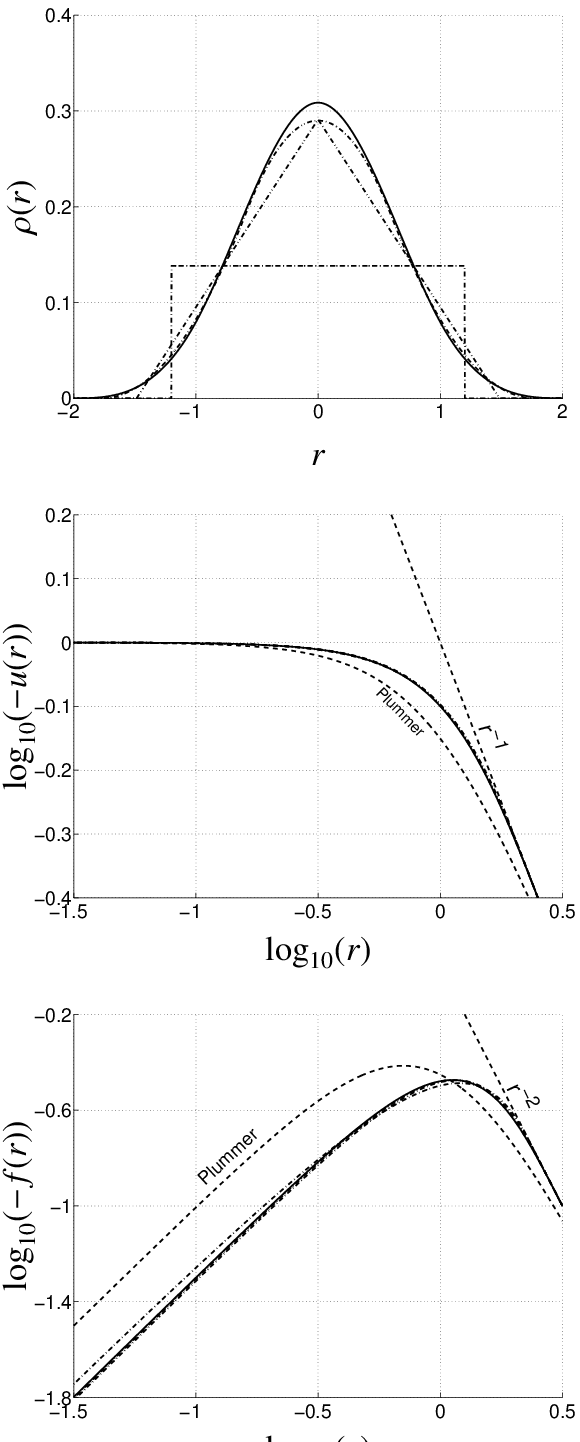
Figure 2 illustrates the density, potential, and force profiles for various at fixed , for pairs of identical particles.
As may be apparent from the figure, as we take the limit at fixed , the density profile converges to a gaussian discussed in section 5. Indeed, as suggested by table in Appendix A.2 the coefficient in Eqn. (17) scales roughly as . Assuming this scaling for , using Eqns.(17), (12), (13), and taking the limit we arrive to the gaussian clouds Eqn. (21).
Next we consider the pairwise force between shaped particles of unequal softening length. Figure 3 shows examples of the force laws between particles of smoothing scales and ; the different panels show different smoothing indices . As the ratio , this approaches the interaction between a cloud and a point particle. As is apparent from the figure, the force profiles quickly converge to the asymptotic () behaviors for both and .

4.3 Spline Softening
As noted above, our density shape corresponds to the spline kernels used in, e.g., SPH [7, 11, 12] smoothing. However the spline force law does not exactly match ours. This is because the spline force used commonly in the literature does not correspond to the force law between two clouds, but rather to the force law between a cloud and a point particle.
In spline softening, interparticle potential and force laws follow from Appendix A.1.2. Zero separation interaction potential becomes
| (19) |
where we have used equation (31) and scaling
| (20) |
It may first appear given the discussion in section 3 that spline softening can be viewed as force between the spherically symmetric clouds of shapes . We can show however that spline softening is inconsistent with such model. Indeed, equations (12) and (13) show is negative for some , hence is imaginary. On the other hand, equation (4) shows that the fourier component of any spherically symmetric cloud is real. By contradiction this proves that there is no possible solution for the density shape that for a pair of identical particles of this shape would under gravitational interaction give us the force law used in the spline force softening.
Whether or not this conclusion brings important consequences for simulations that use spline softening is debatable and is open for future tests. Using the extended Plummer, W-shape or gaussian softenings however allows one to immediately resolve this uncertainty.
5 Gaussian Softening
Gaussian smoothing
| (21) | |||||
| (22) |
allows the simplest expression for softening between clouds of different smoothing scale and, as shown in section 4.2, is the limit of softening with our shapes. For the interaction potential between two gaussian clouds of softenings and whose centers are separated by distance this gives
| (23) |
where
| (24) |
We have found that interaction potential in pair of gaussian clouds of softening scales and equals interaction potential between identical gaussian clouds each having softening scale .
This simple prescription in Eqn. (24) however does not generalize to most other commonly used shapes. For a general cloud shape and general symmetric combination the prescription is valid only if
| (25) |
for all , as can be seen from Eqn. (2). The condition is exact for gaussian clouds and given by Eqn. (24), but is not satisfied for other commonly used shapes: Plummer, spline or W-shapes.
6 Relations between Softenings
In this section, we turn to the relation between our proposed W-shape (we assume ), extended Plummer laws and the more familiar spline, Plummer and gaussian force softenings.
How different, in practice, are our proposed profiles from previously used laws? To answer this, we first must normalize the various profiles to match each other as closely as possible. We do so by matching zero separation interaction potentials in pairs of identical particles. Normalized in this way
| (26) |
which allows us to drop the subscripts. We see from figure 4 that our -shape profiles are quite close to spline and gaussian softening for the same but diverge from Plummer profile.
The close coincidence of W-shape and spline curves is consistent with the idea that our W-shapes reach gaussian in the limit . It may therefore appear first that the prescription of Eqn. (24) is the consistent way to generalize the interparticle laws to pairs of unequal softenings. As a measure of consistency, in figure 5 we plot the force laws found using this prescription against the “correct” force laws found in the result of double integration over particle shapes. The coincidence is identical for gaussian softening (not shown in figure), as we know from section 5.
For Plummer force law the solid lines are found by numerical integration using Eqns. (2) and (9) and the dashed lines are found by plugging into Eqn. (1). From the plot we find this prescription leads to up to relative systematic inconsistency force.
For W-shape softening this prescription results in at most systematic increase over the self-consistent Poisson gravity force law. The latter is however easily computable using the expressions we provided, hence there is no advantage in using the simplification in the first place.


7 Numerical Implementation
The documented WSHAPE package (this paper uses version ) is available at http://www.gracos.org/wshape. We provide numerical C-implementation of the potential and force laws for W-shape and extended Plummer. Also provided within the package is the procedure used to arrive to expressions in Appendix B and values of coefficients in Table 2.
8 Conclusions
An N-body simulation is a simulation of massive particles under the influence of gravity. In cosmological simulation interparticle force is softened to avoid hard collisions. Simulation particles have often been viewed as particles of fixed density shapes in previous literature (e.g. expression for in Eqn. (5) of [11]). To ensure that the nature of interaction between particles in simulations remains gravitational we adpot this interpretation in which force softening corresponds to interaction between cloudlike particles of a fixed density shape.
We prove that the Plummer interparticle force softening is consistent with this force softening model and generalize the Plummer force law into the case of unequal softening scales and .
Interestingly, we mathematically prove that the previosuly used in literature (e.g. [11]) method of spline softening is inconsistent with gravitational interaction in the sense that there is no possible solution for the density shape that for a pair of identical particles of this shape would under gravitational interaction give us the force law used for interparticle force law in spline softening.
We provide the closed form solution for potential and force laws between widely known -cloud shapes of general softenings and .
Our generalized interparticle force laws should be useful for N-body simulations with adaptive mass refinement, in which particles of different mass interact gravitationally. Examples include simulations of the first collapsed objects in the universe [1], the “Via Lactea” simulation [2], pure gravity extension of particle splitting [8], and simulations of dark matter that includes pointlike objects, e.g. stars or supermassive black holes.
As an easy way to extend the force law into pairs of particles of unequal softenings and one would plug their symmetric combination of and as the softening scale . We found that using the simple gaussian motivated recipe for simulations with adaptive mass resolution generally leads to significant systematic uncertainties for the pairs of particles of unequal softenings. The overall effect of these errors can be established by numerical convergence tests similar to [14]. However the problem is immediately resolved by using our proposed profiles.
For convenience, we also made a numeric implementation of our analytic expressions. The most efficient way to use these laws in an N-body simulation would be to pre-compute the interaction law once before running the simulation, and then to interpolate by look-up from the precomputed table. The GRACOS package [15] will implement these profiles for adaptive softening.
Acknowledgments
I thank Neal Dalal for suggesting this topic, and for helpful discussions, in particular for the derivation of the Gaussian limit of the shapes. I thank Pascal Vaudrevange, Pat McDonald, John Dubinski, Norm Murray, Ue-Li Pen, Latham Boyle, Sergei Shandarin and Lev Kofman for helpful discussions. I thank E. Bertschinger for his teaching and guidance on N-body codes. This work was supported by the Canadian Institute for Theoretical Astrophysics (CITA) and the Natural Sciences and Engineering Research Council of Canada (NSERC).
References
- [1] J. Diemand, B. Moore, J. Stadel, Earth-mass dark-matter haloes as the first structures in the early Universe, Nature433 (2005) 389–391.
- [2] J. Diemand, M. Kuhlen, P. Madau, Dark Matter Substructure and Gamma-Ray Annihilation in the Milky Way Halo, ApJ657 (2007) 262–270.
- [3] E. Bertschinger, Multiscale Gaussian Random Fields and Their Application to Cosmological Simulations, ApJS137 (2001) 1–20.
- [4] S. D. M. White, Simulations of merging galaxies, MNRAS184 (1978) 185–203.
- [5] C. Power, J. F. Navarro, A. Jenkins, C. S. Frenk, S. D. M. White, V. Springel, J. Stadel, T. Quinn, The inner structure of CDM haloes - I. A numerical convergence study, MNRAS338 (2003) 14–34.
- [6] Z. Lukic, K. Heitmann, S. Habib, S. Bashinsky, P. M. Ricker, The Halo Mass Function: High Redshift Evolution and Universality, ArXiv Astrophysics e-prints.
- [7] J. J. Monaghan, J. C. Lattanzio, A refined particle method for astrophysical problems, A&A149 (1985) 135–143.
- [8] H. Martel, N. J. Evans, II, P. R. Shapiro, Fragmentation and Evolution of Molecular Clouds. I. Algorithm and First Results, ApJS163 (2006) 122–144.
- [9] I. S. Gradshteyn, I. M. Ryzhik, Table of integrals, series and products, New York: Academic Press, —c1994, 5th ed. completely reset, edited by Jeffrey, Alan, 1994.
- [10] R. W. Hockney, J. W. Eastwood, Computer simulation using particles, Bristol: Hilger, 1988, 1988.
- [11] V. Springel, The cosmological simulation code GADGET-2, MNRAS364 (2005) 1105–1134.
- [12] D. J. Price, J. J. Monaghan, An energy-conserving formalism for adaptive gravitational force softening in smoothed particle hydrodynamics and N-body codes, MNRAS374 (2007) 1347–1358.
- [13] R. Ferrell, E. Bertschinger, Particle-Mesh Methods on the Connection Machine, Contributions to Mineralogy and Petrology (1993) 10002–+.
- [14] K. Heitmann, P. M. Ricker, M. S. Warren, S. Habib, Robustness of Cosmological Simulations. I. Large-Scale Structure, ApJS160 (2005) 28–58.
- [15] A. Shirokov, E. Bertschinger, GRACOS: Scalable and Load Balanced P3M Cosmological N-body Code, ArXiv Astrophysics e-prints.
Appendix A Force and Potential Law in a Pair of Cloud Shapes
This section provides closed form expressions (for ) for interaction potential laws in a pair of two cloud shapes of scales and , a pair of two identical -shape particles of scale , and a pair consisting of an -shape particles and a point-like particle. Interparticle force laws follow immediately by differentiation with respect to separation and flipping the sign.
A.1 Analytic Expression
A.1.1 Two Parametric Form
Potential law for interaction in a pair of two -shape particles of scales and and a fixed is given by Eqn. (14). Its closed form solution is given as a finite sum over all integers and , with
| (27) |
where for , and the values of positive integers and are given for each in Appendix B.
Coefficients depend on through the Heaviside function via summation over all integers and
| (28) |
where for integers and , and are constant non-zero integer coefficients, whose complete set for each is presented in Appendix B. The total number of terms in these expressions is finite. The potential is symmetric with respect to and , as should be.
A.1.2 One Parametric Forms
Potential laws for interaction in a pair of two identical -shape particles of scale (case ), or one -shape particle of scale and a point-like particle (case ) are found in Eqn. (16) and (15). Their closed form solutions are given by
| (29) |
where . The values of positive integers and are given for each and in Appendix B. Coefficients depend on through the Heaviside function via
| (30) |
where for an integer , and are constant non-zero integer coefficients, whose complete set for each is also presented in Appendix B.
A.2 Asymptotic Expressions
Potential laws in section A.1 are pure Newtonian beyond separation distance when particle last overlap. Indeed at , and at . On the other hand, for small separations we have analytically for
| (31) |
where numerical values of coefficients are given in Tables 2.
Figure 6 shows the density, potential and force laws for for pair of identical particles of smoothing scale . Note the different amplitudes for the potential and linear force law at small for different , which is consistent with growing values of and for .

Appendix B Tables of Coefficients
This subsection provides tables of coefficients for analytic expressions for potentials in Section A.1 for . The procedure used to find these table values is given in Appendix 7.
B.1 Spherical Top-hat – Shaped Particles (-Shape)
Values , are applicable for the entire subsection B.1.
B.1.1 Point-like Test Particle
The following table lists values of coefficients ; the numbers, labeling the rows and columns denote and .
B.1.2 Identical Particles
The following table lists values of coefficients ; the numbers, labeling the rows and columns denote and .
B.1.3 General Case
The following two tables list values of coefficients and ; the numbers, labeling the rows and columns denote and .
The rest of the non zero coefficients in Eqn. (28) are given by the following relations
B.2 Cone – Shaped Particles (-Shape)
Values , are applicable for the entire subsection B.2.
B.2.1 Point-like Test Particle
The following table lists values of coefficients ; the numbers labeling the rows and columns denote and .
B.2.2 Identical Particles
The following table lists values of coefficients ; the numbers, labeling the rows and columns in the following table, denote and respectively.
B.2.3 General Case
The following three tables list values of coefficients , , and ; the numbers, labeling the rows and columns denote and respectively.
The rest of the non zero coefficients are given by the following relations.
B.3 TSC-Shape Particles (-Shape)
Values , are applicable for the entire subsection B.3.
B.3.1 Point-like Test Particle
The following table lists values of coefficients ; the numbers, labeling the rows and columns denote and respectively.
B.3.2 Identical Particles
Table 4 lists values of coefficients .
B.3.3 General Case
Table 4 lists values of coefficients . The rest of the non zero coefficients are given by the following relations
B.4 Cubic Spline - Shaped Particles ( -Shape)
Values , are applicable for the entire subsection B.4.
B.4.1 Point-like Test Particle
The following table lists values of coefficients ; the numbers, labeling the rows and columns denote and .
B.4.2 Identical Particles
Table 6 lists values of coefficients .
B.4.3 General Case
Table 6 lists values of coefficients , and . The rest of the coefficients are given by the following relations: