WUB/07-10
New Higgs mechanism from the lattice

Gauge theories in dimensions $d>4$ are (part of) models, which aim at explaining the origin of the Higgs field and electroweak symmetry breaking, one of Gauguin’s questions in particle physics [1] that has been reviewed at this conference [2]. In such extensions of the Standard Model based on gauge-Higgs unification the Higgs is identified with extra-dimensional components of a gauge field. The Higgs potential is zero at tree level and is generated through quantum effects [3]. The Higgs mass and quartic coupling, which are inputs of the Standard Model, become dynamical properties. In case of non-simply connected extra-dimensional spaces, like a circle $S^{1}$ or a torus $T^{2}$, the physical degrees of freedom of the Higgs actually reside in the non-contractible Polyakov loops. It is argued that the Higgs potential is finite [4] despite the non-renormalizability of the models, the intuitive reason being that non-local counterterms are not allowed. The potential can further break spontaneously the gauge symmetry. This extra-dimensional version of the Higgs mechanism is referred as the Hosotani mechanism [5, 6].

A particularly simple and attractive extra-dimensional space is the orbifold $S^{1}/\mathbb{Z}_{2}$. The $\mathbb{Z}_{2}$ projection identifies degrees of freedom under the reflection of the fifth dimensional coordinate. The circle $S^{1}$ is thus projected onto an interval $I_{1}$. Gauge fields are identified under this reflection up to a global gauge transformation. The ends of the interval are the fixed points of the reflection and naturally define boundaries. It turns out that there is a tower of boundary conditions for the gauge field and its derivatives, which can be derived as a limit of a gauge invariant construction [7]. In this limit the gauge invariance is broken on the boundaries. For the purpose of recovering the Standard Model Higgs this explicit breaking of the gauge symmetry allows to get a Higgs field which is not in the adjoint representation of the gauge group: some of the extra-dimensional components of the gauge field are set to zero at the boundaries and therefore do not have a zero-mode. If we think of dimensional reduction as in finite temperature field theory, the low-energy effective theory is described by zero-modes and we end up with a Higgs field in the fundamental representation of a subgroup of the original gauge group.

Five-dimensional gauge theories formulated on $S^{1}/\mathbb{Z}_{2}$ can be studied using perturbation theory. One starts with a Fourier or Kaluza–Klein (KK) expansion of the gauge field, each gauge field component is associated with a tower of four-dimensional fields but only some (even) components have a zero-mode. The 1-loop expression for the Higgs mass $m_{H}$ for general gauge group $SU(N)$ is [8, 9]

$\displaystyle(m_{H}R)^{2}$

$\displaystyle=$

$\displaystyle\frac{9N\zeta(3)}{32\pi^{4}}g_{4}^{2}\,,\quad g_{4}^{2}\,=\,\frac{g_{5}^{2}}{2\pi R}\,,$

(1)

where $R$ is the radius of the extra dimension and $g_{5}$, $g_{4}$ are the five-dimensional and effective four-dimensional gauge couplings respectively. This expression agrees with the one obtained from the computation of the effective potential at 1-loop [10]. This fact we find remarkable, since the 1-loop potential is an effective potential for free fields and the gauge coupling there only enters indirectly through the shifted masses of the Kaluza–Klein modes. The minimization of the potential also shows that there is no spontaneous symmetry breaking (at 1-loop). This observation led to consider models where (a large number of) bulk fermion fields are added to trigger spontaneous symmetry breaking. We found it appropriate to pause for a moment and look in detail at how the perturbative computations have been done.

Perturbative computations of the effective scalar potential in five-dimensional gauge theories consist of two steps: diagonalization of the mass matrix for the KK modes and (re)summation of their 1-loop contributions to the effective action.

The first step is done by expanding the five-dimensional fields in a Fourier basis on $S^{1}/\mathbb{Z}_{2}$. The orbifold boundary conditions determine which gauge field component is even and which is odd,

	$\displaystyle E(x,x_{5})$	$\displaystyle=$	$\displaystyle\frac{1}{\sqrt{2\pi R}}E^{(0)}(x)+\frac{1}{\sqrt{\pi R}}\sum_{n=1}^{\infty}E^{(n)}(x)\cos(nx_{5}/R)\quad\mbox{even fields}\,,$		(2)
	$\displaystyle O(x,x_{5})$	$\displaystyle=$	$\displaystyle\frac{1}{\sqrt{\pi R}}\sum_{n=1}^{\infty}O^{(n)}(x)\sin(nx_{5}/R)\quad\mbox{odd fields}\,.$		(3)

Dimensional reduction is expected to occur for energies $E\ll 1/R$, where physics is described by a low-energy effective theory of zero-modes $E^{(0)}$. This expectation has to be verified by computations of low-energy physical quantities. The mode expansion of the fields is inserted in the lagrangean

$\displaystyle-\cal L$

$\displaystyle=$

$\displaystyle\frac{1}{2g_{5}^{2}}{\rm tr}\{F_{MN}F_{MN}\}+\frac{1}{g_{5}^{2}\xi}{\rm tr}\{(\bar{D}_{M}A_{M})^{2}$

(4)

with $\bar{D}_{M}F=\partial_{M}F+[\langle A_{M}\rangle,F]$ and we set $\xi=1$ (unexplained notation is as in [11]). From a four-dimensional point of view, the five-dimensional components of the gauge field $A_{5}$ are scalars and can assume a vacuum expectation value (vev) $\langle A_{5}\rangle\neq 0$. The masses of the KK modes are found by diagonalization of the operator $\bar{D}_{5}\bar{D}_{5}$. In order to give a concrete example we consider the gauge group $SU(2)$ with the orbifold breaking

$\displaystyle SU(2)$

$\displaystyle\stackrel{{\scriptstyle\mathbb{Z}_{2}}}{{\longrightarrow}}$

$\displaystyle U(1)$

(5)

The KK masses are

	$\displaystyle A_{\mu}^{3,(0)}\ (\mbox{gauge boson}):$	$\displaystyle(m_{Z}R)^{2}=\alpha^{2}$			(6)
	$\displaystyle A_{5}^{1,2(0)}\ (\mbox{Higgs}):$	$\displaystyle(m_{A_{5}}R)^{2}=\alpha^{2}\,,\;0$			(7)
	$\displaystyle\mbox{higher KK modes}:$	$\displaystyle(m_{n}R)^{2}=n^{2}\,,\;(n\pm\alpha)^{2}$			(8)

where

$\displaystyle\alpha\,=\,g_{5}\langle A_{5}^{1}\rangle R\,=\,g_{5}vR/\sqrt{2\pi R}$

(9)

is a dimensionless modulus parametrizing the four-dimensional Higgs vev $v$.

The second step is to sum the four-dimensional 1-loop effective action for the KK modes. This step involves a Poisson resummation which eliminates a constant (i.e. independent of $\alpha$) divergent contribution. The result is the periodic potential

$\displaystyle V$

$\displaystyle=$

$\displaystyle-\frac{9}{64\pi^{6}R^{4}}\sum_{m=1}^{\infty}\frac{\cos(2\pi m\alpha)}{m^{5}}\,,$

(10)

which has degenerate minima at $\alpha=\alpha_{\rm min}=0\;{\rm mod}\,\mathbb{Z}$. For these values of $\alpha$ the spectrum as a whole is the same as for $\alpha=0$. There is no spontaneous symmetry breaking of the remnant $U(1)$ gauge symmetry in Eq. (5), which would manifest itself in a massive lowest mode for $A_{\mu}^{3}$.

The orbifold theory with the explicit symmetry breaking Eq. (5) can be defined on a Euclidean space-time lattice [7]. The geometry is the strip $\{z=a(n_{\mu},n_{5})|\;0\leq n_{5}\leq N_{5}\}$, where $a$ is the lattice spacing, the integer coordinates $n_{\mu}$ label points in a four-dimensional hypercube $\frac{T}{a}\times(\frac{L}{a})^{3}$ and $n_{5}=0,\;N_{5}$ define the boundaries. The parameter space on the lattice is given by

$\displaystyle N_{5}\;=\;\pi R\Lambda\quad\mbox{and}\quad\beta=2N/(g_{5}^{2}\Lambda)\,,$

(11)

where $\Lambda=1/a$ is the ultraviolet cut-off. Details on the lattice action and operators can be found in [12]. It turns out that there is a first order phase transition at $\beta_{c}\simeq 1.6$. This transition is the same as the one observed in infinite volume (or with periodic boundary conditions) [13, 14, 15, 16] and can be detected by a jump in the expectation value of the plaquettes. We did a mean-field calculation [17] that also shows the presence of the phase transition and reproduces the qualitative behavior of the plaquettes, see figure 2. The spectrum of the scalar (Higgs/glueball) and vector (gauge boson) states can only be measured in simulations for $\beta>\beta_{c}$ and is shown in figure 2 for $N_{5}=6$ as a function of $\beta$. The Higgs mass is larger then the 1-loop continuum value Eq. (1). The gauge boson is a massive $Z$ boson, contrary to the perturbative result that we discussed in the previous section. This is the first lattice evidence for spontaneous symmetry breaking in pure extra-dimensional gauge theories [18]. The appearance of a Higgs phase is not completely unexpected from dimensional reduction [19].

Five-dimensional gauge theories are trivial: if a ultraviolet cut-off $\Lambda$ is removed from the theory, the four-dimensional effective coupling $g_{4}$ goes to zero [20], see also [21, 22]. In this limit the Higgs mass Eq. (1) tends to zero. In order to move away from the trivial limit we regularize the theory on a Euclidean lattice, which naturally provides a gauge invariant cut-off $\Lambda=1/a$. We make the hypothesis that in a vicinity of the trivial point the lattice theory can be described by a continuum Symanzik effective lagrangean

$\displaystyle-{\cal L}$

$\displaystyle=$

$\displaystyle\frac{1}{2g_{5}^{2}}{\rm tr}\{F_{MN}F_{MN}\}+\sum_{p_{i}}{c^{(p_{i})}(N_{5},\beta)}\;{a^{p_{i}-4}}\;{\cal O}^{(p_{i})}+\ldots\,,$

(12)

where ${\cal O}^{(p_{i})}$ is an operator of dimension $p_{i}>4$. This expansion has been shown to describe cut-off effects for renormalizable theories [23, 24, 25, 26]. Our working hypothesis is that the five-dimensional gauge theory, despite its non-renormalizability, possesses a scaling regime where it is described by Eq. (12).

For the orbifold the operators of lowest dimension are

	$\displaystyle c_{0}\,{\cal O}^{(5)}$	$\displaystyle=$	$\displaystyle\frac{\pi a{c}_{0}}{4}F_{5\mu}^{\hat{a}}F_{5\mu}^{\hat{a}}\left[\delta(x_{5})+\delta(x_{5}-\pi R)\right]\,,$		(13)
	$\displaystyle c\,{\cal O}^{(6)}$	$\displaystyle=$	$\displaystyle\sum_{M,N}\frac{c}{2}{\rm tr}\{F_{MN}(D_{M}^{2}+D_{N}^{2})F_{MN}\}\,,$		(14)

where the coefficients $c_{0}\equiv c^{(5)}(N_{5},\beta)$ and $c\equiv c^{(6)}(N_{5},\beta)$ depend on the lattice gauge action and can be computed in perturbation theory. For example $c=1/12$ at tree level for the Wilson plaquette action. Higher derivative operators like Eq. (14) appear in models for new Higgs physics considered in [27, 28], where they are interpreted as new particles (ghosts) which cancel quadratic divergences in the Higgs mass.

The operators Eq. (13) and Eq. (14) induce corrections to the KK masses of the gauge field $A_{\mu}$. For example Eq. (6) and Eq. (8) in the $SU(2)$ model are changed to

	$\displaystyle(m_{n}R)^{2}=$		$\displaystyle n^{2}\,,\qquad\mbox{for}\;n>0\,,$		(15)
			$\displaystyle(n\pm\alpha)^{2}+\frac{c_{0}\alpha^{2}}{2}\frac{\pi}{N_{5}}+c\,(n\pm\alpha)^{4}\frac{\pi^{2}}{N_{5}^{2}}\qquad\mbox{for}\;n\geq 0\,,$		(16)

where we keep only the leading $n$-independent correction from the boundary term. The gauge field $A_{5}$ and the ghost field do not receive cut-off corrections, since the masses of their KK modes originate from the gauge fixing term.

When inserted into the formula for the Higgs potential, the corrected KK masses Eq. (16) lead to an expansion in $c_{0}$ and $c$ of the $A_{\mu}$ (gauge) contribution [11]. The latter is defined as

$\displaystyle V^{\rm gauge}$

$\displaystyle=$

$\displaystyle-\frac{1}{2}\sum_{n\in\mathbb{Z}}\int\limits_{0}^{\infty}\frac{{\rm d}l}{l}{\rm e}^{-\frac{1}{l}(m_{n}^{2}a^{2}+8)}\frac{1}{a^{4}}{\rm I}_{0}^{4}\left(\frac{2}{l}\right)\,.$

(17)

A tricky point here is that we extend the summation over a finite number of KK modes on the lattice to $n\to\infty$, but this is justified since the contribution of higher modes is exponentially suppressed in Eq. (17). The expansion then reads

$\displaystyle V^{\rm gauge}$

$\displaystyle=$

$\displaystyle f_{0}+\underbrace{c_{0}f_{1}}_{{\rm O}(a)}+\underbrace{c_{0}^{2}\tilde{f}_{2}+cf_{2}}_{{\rm O}(a^{2})}$

(18)

and the total potential is given by

$\displaystyle V$

$\displaystyle=$

$\displaystyle\underbrace{4V^{\rm gauge}}_{A_{\mu}}\underbrace{+V^{\rm scalar}}_{A_{5}}\underbrace{-2V^{\rm scalar}}_{\mbox{ghosts}}\,.$

(19)

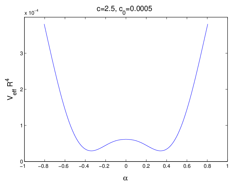
Here $V^{\rm scalar}$ is obtained by setting $c=c_{0}=0$ in Eq. (17). The cut-off corrected effective potential for $N_{5}=6$, $c=2.5$ and $c_{0}=0.0005$ is shown in figure 3. For each value of $N_{5}$ and $c_{0}=0$, there is a minimal positive value of $c$ such that there is spontaneous symmetry breaking [29]: the minimum of the potential is attained at $\alpha_{\rm min}=1/2$. When in addition $c_{0}>0$, the potential is not any more periodic in $\alpha$. The requirement that the vev is below the cut-off scale: $v<1/a$ implies the constraint $|\alpha|<\sqrt{NN_{5}/(\pi^{2}\beta)}$. The Higgs potential has the characteristic shape like in the Standard Model as shown figure 3 and the minimum is shifted continuously in the range $0<\alpha_{\rm min}<1$ depending on the value of $c_{0}$.

We are now in the position to compare the results from cut-off corrected perturbation theory with the lattice simulations of the orbifold with bulk gauge group $SU(2)$. This should provide the justification for our working hypothesis of using the Symanzik expansion. In figure 5 we compare for $N_{5}=6$ the masses of the $Z$ and $Z^{*}$ bosons as a function of the modulus $\alpha_{\rm min}$. The lines represent the formulae Eq. (16) for $n=0,1$ for fixed values $c=13.0$ and $c_{0}=0.0121$ varying $\alpha=\alpha_{\rm min}$. Actually for these values of $c$ and $c_{0}$ the potential has a minimum at the position indicated by the vertical dotted line. The symbols are the simulation results of the orbifold with $T/a=96$, $L/a=12$, $N_{5}=6$, plotted using a lattice determination of $\alpha_{\rm min}$ [11]. There is good qualitative agreement.

In figure 5 we compare always for $N_{5}=6$ the ratio of the Higgs to the Z-boson mass $\rho_{HZ^{0}}=m_{H}/m_{Z^{0}}$. Here $c$ and $c_{0}$ in the potential calculation are tuned to give the minimum at the value $\alpha_{\rm min}$ as it is determined in the lattice simulation. The perturbative results for $\rho_{HZ^{0}}$ are represented by the square symbols. The lattice results (circles and triangles, orbifold with $T/a=96$, $L/a=12$ and $L/a=14$, $N_{5}=6$) indicate that contrary to perturbation theory on the lattice it is possible to get $\rho_{HZ^{0}}\geq 1$.

We are investigating five-dimensional gauge theories as models to derive electroweak symmetry breaking, by a combination of lattice simulations and analytic computations. We gave the first evidence for spontaneous symmetry breaking and could reproduce this effect by the inclusion of cut-off effects in perturbation theory. Our results encourage to pursue the study in order to establish whether these theories possesses a scaling regime, where the values of physical observables do not strongly depend on the cut-off.

References

- [1] Ellis J 2007 (Preprint arXiv:0710.5590 [hep-ph])
- [2] Giudice G F 2007 (Preprint arXiv:0710.3294 [hep-ph])
- [3] Coleman S R and Weinberg E 1973 Phys. Rev. D7 1888–1910
- [4] Antoniadis I, Benakli K and Quiros M 2001 New J. Phys. 3 20 (Preprint hep-th/0108005)
- [5] Hosotani Y 1983 Phys. Lett. B126 309
- [6] Hosotani Y 1989 Ann. Phys. 190 233
- [7] Irges N and Knechtli F 2005 Nucl. Phys. B719 121–139 (Preprint hep-lat/0411018)
- [8] von Gersdorff G, Irges N and Quiros M 2002 Nucl. Phys. B635 127–157 (Preprint hep-th/0204223)
- [9] Cheng H C, Matchev K T and Schmaltz M 2002 Phys. Rev. D66 036005 (Preprint hep-ph/0204342)
- [10] Kubo M, Lim C S and Yamashita H 2002 Mod. Phys. Lett. A17 2249–2264 (Preprint hep-ph/0111327)
- [11] Irges N, Knechtli F and Luz M 2007 JHEP 08 028 (Preprint arXiv:0706.3806 [hep-ph])
- [12] Irges N and Knechtli F 2007 Nucl. Phys. B775 283–311 (Preprint hep-lat/0609045)
- [13] Creutz M 1979 Phys. Rev. Lett. 43 553–556
- [14] Beard B B et al. 1998 Nucl. Phys. Proc. Suppl. 63 775–789 (Preprint hep-lat/9709120)
- [15] Ejiri S, Kubo J and Murata M 2000 Phys. Rev. D62 105025 (Preprint hep-ph/0006217)
- [16] Farakos K, de Forcrand P, Korthals Altes C P, Laine M and Vettorazzo M 2003 Nucl. Phys. B655 170–184 (Preprint hep-ph/0207343)
- [17] Knechtli F, Bunk B and Irges N 2006 PoS LAT2005 280 (Preprint hep-lat/0509071)
- [18] Irges N and Knechtli F 2006 (Preprint hep-lat/0604006)
- [19] Fradkin E H and Shenker S H 1979 Phys. Rev. D19 3682
- [20] Dienes K R, Dudas E and Gherghetta T 1999 Nucl. Phys. B537 47–108 (Preprint hep-ph/9806292)
- [21] Gies H 2003 Phys. Rev. D68 085015 (Preprint hep-th/0305208)
- [22] Morris T R 2005 JHEP 01 002 (Preprint hep-ph/0410142)
- [23] Symanzik K 1982 Mathematical Problems in Theoretical Physics, eds. R. Schrader et al., Lecture Notes in Physics 153 47–58 presented at 6th Int. Conf. on Mathematical Physics, Berlin, West Germany, Aug 11-21, 1981
- [24] Symanzik K 1983 Nucl. Phys. B226 187
- [25] Symanzik K 1983 Nucl. Phys. B226 205
- [26] Lüscher M 1998 (Preprint hep-lat/9802029)
- [27] Grinstein B, O’Connell D and Wise M B 2007 (Preprint arXiv:0704.1845 [hep-ph])
- [28] Fodor Z, Holland K, Kuti J, Nogradi D and Schroeder C 2007 (Preprint arXiv:0710.3151 [hep-lat])
- [29] Luz M, Knechtli F and Irges N 2007 (Preprint arXiv:0709.4549 [hep-lat])