Uniformizing Tropical Curves I: Genus Zero and One
Abstract.
In tropical geometry, given a curve in a toric variety, one defines a corresponding graph embedded in Euclidean space. We study the problem of reversing this process for curves of genus zero and one. Our methods focus on describing curves by parameterizations, not by their defining equations; we give parameterizations by rational functions in the genus zero case and by non-archimedean elliptic functions in the genus one case. For genus zero curves, those graphs which can be lifted can be characterized in a completely combinatorial manner. For genus one curves, show that certain conditions identified by Mikhalkin are sufficient and we also identify a new necessary condition.
In the past five years, a group of mathematicians, lead by Grigory Mikhalkin, have pioneered a new method for studying curves in toric varieties. According to this perspective, one considers curves defined over a field with a non-archimedean valuation. Using this valuation and an embedding of a curve into an (algebraic) torus, one constructs a graph embedded in a real vector space. This graph is known as the tropicalization of the curve. From the tropicialization of , one tries to read off information about the degree and genus of the original curve , and its intersections with other subvarieties of the torus. In this introduction, we will write for a curve embedded in a torus and we will write for the tropicalization of .
In order to use these tropical methods, we need to know which graphs are tropicalizations of curves. We will refer to a graph which actually is the tropicalization of a curve as a tropical curve. There are certain basic combinatorial conditions which hold for any tropical curve. The first, the zero tension condition, is a description of the possible local structures of a tropical curve around a given vertex. (See the beginning of Section 3.) We can assign to a multiset of lattice vectors, which we will call the degree of , from which we can determine the homology class represented by the closure of when this closure is taken in a suitable toric compactification of . The second combinatorial condition is that the directions of the unbounded rays of are given by the degree of . (See Section 1.) Thirdly, we can show that, modulo some technical conditions, the genus of is greater than or equal to the first Betti number of . (See Theorem 10.8.) We will define a zero-tension curve of genus and degree to be a graph which has first Betti number and obeys the obvious conditions to be the tropicalization of a degree curve.
We attack the reverse problem: Given a zero-tension curve of genus and degree , when does it come from an actual curve of genus and degree ? The main contribution of this paper is to show that methods of non-archimedean analysis can be used to construct algebraic curves with a given tropicalization. In this paper, we will consider this question for genus zero and genus one curves. In the sequel, we will describe the corresponding results for higher genus curves, where we will need to use Mumford’s uniformization results. A second achievement of this paper is to describe an obstruction to lifting zero-tension curves of genus one – the condition of being well spaced – which is more subtle that than those mentioned above but is still combinatorial and easy to test.
I want to state clearly that there is a major difficulty in directly using these results for enumerative purposes involving curves of positive genus. If is a curve of genus , than the tropicalization of is a zero-tension curve with first Betti number less than or equal to . Therefore, if we want to count genus curves with obeying some conditions, we should look at all zero-tension curves of genus less than or equal to , and determine which of them lift to actual genus curves obeying the condition (and in how many ways the lifting can be done). However, we have almost no results restricting the capability to lift a tropical curve whose first Betti number is strictly less than to an actual curve of genus . When studying curves in toric surfaces, one can use basic dimension counting arguments to show that there are no such contributions, but this cannot be done for curves in higher dimensional toric varieties. We expect, therefore, that the primary use of these results will not be to prove exact combinatorial formulas, but rather to provide existence results or lower bounds.
The idea of studying curves via tropical varieties was proposed by Kontsevich and pioneered by Mikhalkin [14], [15]. In Mikhalkin’s view, tropical varieteis should be seen as spectra of semirings, built from the semiring of the real numbers under the operations and . He also points out, however, that they can be described using valuations over a nonarchimedean field. (As we do here.) Mikhalkin has proven our main theorems, in any genus, in the case of curves in toric surfaces. A purely algebraic proof was given by Shustin and Tyomkin [21]. Since Mikhlkain’s work, there has been a great deal of research extending his results to more sophisticated enumerative problems concerning curves in toric surfaces. There has been far less work on curves in higher dimensional toric varieties. The most important exception is the work of Nishinou and Siebert [18], who use log geometry to analyze the case of genus zero curves and recover essentially all of our results in that case. Finally, we should note that H. Markwig and her collaborators, especially Gathmann, have done major work building the tropical analogue of the moduli spaces of curves and of stable maps and studying it from a combinatorial persepective, see [7] and the works cited therein. Among their results is reestablishing the validity of the tropical enumeration of curves in by showing it matches the Caporaso-Harris formula. The moduli space of tropical genus zero curves was previously described by Mikhalkin in [16].
This paper, which has been several years in preparation, stems from portions of my Ph.D. dissertation. I am extremely grateful to my advisor Bernd Sturmfels, for his guidance in the writing of the dissertation and afterwards. In addition, I am grateful to Paul Hacking, Thomas Markwig, Grigory Mikhalkin, Sam Payne and Jenia Tevelev for many discussions of my work and theirs, including informing me of many results which were unpublished at the time. During the writing of this paper, I have been supported by a research fellowship from the Clay Mathematics Institute.
1. Curves in Toric Varieties
In this section, we will describe how to assign a degree to a curve given with a map to an (algebraic) torus. Throughout this paper, we will write for the lattice of one parameter subgroups of the torus. We will call the dimension of the torus . We write for the torus, or when we want to specify the ground field and the lattice .
Let be a complete rational fan in and let be the associated toric variety over an algebraically closed field . (See [5] for background on toric varieties.) The open torus in is canonically . For each ray (one dimensional cone) of , there is a unique minimal element of on this ray; if we identify with then the element in question is the unique point of the ray whose coordinates are integers with no common factor. Let , …, be the set of minimal vectors of the rays of . The following is a special case of Theorem 3.1 of [6].
Proposition 1.1.
With the notation above, the Chow group is given by
This is a subgroup of , and equals if is smooth.
Let be a smooth, complete algebraic curve and let be a map from into . Let denote , the part of which is mapped to the big torus. Let us say that is torically transverse if is nonempty and is disjoint from the toric strata of codimension and higher. (This is a specialization of the definition of torically transverse in [18].)
For each ray of , let be the codimension stratum of associated to . Let be the length of , in other words, the number of points in counted with multiplicity. Then satisfies11 1 In two paragraphs, we will see an alternate description of the which makes this clear. and hence corresponds to a class in . Capping with the fundamental class gives the class in , and hence in , corresponding to . Thus, if we want to study torically transverse curves representing a particular class in , we may begin by finding the possible preimages of this class in and studying curves of that degree.
Continue to assume that is torically transverse. Let . We now describe how to determine which ray of corresponds to , and with what multiplicity, solely by examining the map . Namely, for , let be the function on corresponding to . Then is a function on and it extends to a meromorphic function on . Let be the order of vanishing of this function at . Then is a linear map and thus an element of . If then extends to , contradicting our choice that lies in . Instead, is a nonzero element of . Write as where is a positive integer and is minimal. Then is the ray of corresponding to and is the multiplicity.
We now make a definition: let be a smooth algebraic curve and let be an algebraic map. (Whenever is nonconstant, the curve is not complete.) Let be the smooth complete curve compactifying ; we impose the condition that can not be extended to any point of . Let be any point of . Define , and as before. Let , …, be the set of distinct values of as ranges over . For , let and set . We define the set to be the degree of . Note that this is defined without any choice of toric compactification of . Note also that we have , because any rational function has equally many zeroes and poles on .
We then have:
Proposition 1.2.
Let be a complete fan with rays generated by , …, and let be any class in . Then there is a bijection between torically transverse curves which represent the given class and maps which are incapable of being extended to any larger compactficiation of and have degree ; this bijection is given by restriction to the preimage of in .
For this reason, we can reformulate questions about constructing torically transverse curves in toric varieties into questions about constructing curves of given degree in torii. Ordinarily, of course, one wishes to consider all curves in some toric variety, not only the torically transverse ones. In many applications, it can be shown by dimensional considerations that all of the curves of interest are torically transverse. Even when this is not true, it is true that, if we specify the cohomology class of a curve in , then there are only finitely many possible degrees for curves realizing that cohomology class and not lying in the toric boundary – and those curves which do lie in the toric boundary are in the interiors of smaller toric varieties. For this reason, in this paper we will study problems where we specify the degree of a curve in the torus rather than specifying degrees in a toric compactification.
2. Basic Tropical Background
Before introducing any algebraic technology, we discuss an issue concerning polyhedral terminology. In this paper, we will study a great number of polyhedra. All of these will be rational polyhedra, meaning that they are defined by finitely many inequalities of the form where is an integer vector and is a rational number. It will be most convenient to consider these as subsets of . (For example, in Theorem 2.2.) However, we want to be able to use topological language to talk about polyhedral complexes. We therefore adopt the following conventions: a polyhedron is a subset of , defined by finitely many inequalities as above. When we refer to a point of a polyhedron, we mean a point of . Nonetheless, when we describe a polyhedral complex using topological terms, such as “connected”, “simply connected” and so forth, we will mean the properties of the closure of that complex in . Similar issues will arise concerning metrized graphs. We adopt the conventions that the edges of a metrized graph always have rational lengths and that, the points of this graph, considered as a metric space, are the points which have rational distances from all of the vertices. Nevertheless, we will freely speak of graphs as connected, as mapping continuously from one to another, and so forth.
Let be a complete discrete valuation ring with valuation . We write for the fraction field of and for the residue field. We always assume that is algebraically closed. Let be the algebraic closure of , let be the extension of to , let be the ring and and be the maximal ideals of and respectively. Note that, since is algebraically closed, the residue field is also equal to . As our notation suggests, we will primarily consider the objects , and and only occasionally need to deal with , and .22 2 Several earlier tropical works, including some of my own work, attempted to ignore , and entirely. The reader should still view these objects as being only technicial crutches. However, I have become convinced that it is not worth trying to avoid them completely. The first problem is that, is not noetherian. This has never caused any irreperable difficulties, but it slows down work by making standard results inapplicable. Second, one of my motivations for avoiding the boldfaced objects was to be able to work with other fields with valuation, such as the field of those Puiseaux series over that have some positive radius of convergence. In the current paper, however, we will need to have a field complete with respect to . I don’t know of any useful examples where is complete that are not some sort of completion of the algebraic closure of some . We fix a group homorphism from giving a section of ; this is always possible because is surjective and is divisible.33 3 It is quite possible to do without this choice, and Sam Payne has advocated doing so. This is doubtless the most morally correct way of proceeding, but it introduces a great deal of notational baggage. In particular, we would be forced to replace torii with principal homogeneous spaces over torii in several places, and would thus no longer have explicit coordinates.
Let and let . We can write , where is a finite subset of and each is a nonzero element of . Let be the subset of on which the function achieves its minimum. (Here is the pairing .) We define where is the projection . (We set .)
Suppose that we have an injection of rings with for . Suppose also that each coefficient of lies in . Then we can describe more simply as ; note that we sum over , not over . This is the definition that is used in Gröbner theory, where the field is left hidden in the background. Using this alternate definition, we can define for and , even without choosing a field to use. We will say that is a power-series field if we are given such a section . If is a power series field, we will say that a polynomial has constant coefficients if its coefficients lie in the image of and that a variety has constant coefficients if it is defined by polynomials with constant coefficients.
If is an ideal in , let denote the ideal of generated by for . If is the closed subscheme of corresponding to then we write for the closed subscheme of corresponding to . The geometric meaning of is the following: let denote the element of described by for . Consider the subvariety of where denotes the standard action of on itself. Let be the (Zariski) closure of in . Then is the fiber of over . Moreover, suppose that and that is defined over , meaning that there is a subscheme of such that . (Note that we can always achieve these hypotheses by replacing with a finite extension.) Then we may instead describe by taking the Zariski closure of in .
If is an ideal of , rather than of , and any point of then we can define to be the ideal in generated by for all , where is defined by the alternate definition two paragraphs above. While this is a slight abuse of notation, it should cause no confusion: one meaning of is defined for and the other for and the meanings are extremely closely related. Specifically, let be an ideal of , let and let be any power seres field with associated notation . Suppose that and that . Then .
The following lemma will be of frequent use:
Lemma 2.1.
Let be an ideal of . Let and be elements of . Then, for any sufficiently small rational number , we have .
Proof.
This is proved in a slightly less general context as Proposition 1.13 in [25]; the proof can be adapted to our setting. ∎
We now define tropicalization.
Proposition 2.2.
Let be a closed subscheme of and let be the corresponding ideal. Let . Then the following are equivalent:
- (1)
There is a point with .
- (2)
There is a valuation extending with the property that for every in .
- (3)
For every , the polynomial is not a monomial.
- (4)
The ideal does not contain any monomial.
- (5)
The scheme is nonempty.
Note that, in conditions (3) and (4), zero is not considered a monomial.
Proof.
The equivalence of (1), (3) and (4) is Theorem 2.1 of [24]. A very careful and detailed version of this result, by reduction to the hypersurface case, is in [19]. The equivalence of (4) and (5) is simply the Nullstellansatz – since monomials are units in , the ideal contains a monomial if and only if it is all of . The equivalence of (2) and (5) is Theorem 2.2.5 of [3]. ∎
Define the subset of where any of the equivalent conditions above holds to be . Note that condition (3) of the above proposition clearly singles out a closed set. If is a power series field and has constant coefficients, then we can define using the definition of which is defined for . There is little risk of confusion in defining both for and . The precise relation is as follows: Let be any power series field, with associated notation such that and let be a closed subscheme of . Then . The next proposition summarizes basic results on the structure of .
Proposition 2.3.
Let . Then can be given the structure of a polyhedral complex (with finitely many faces). Furthermore, we may do this in such a way that, for any face of this polyhedral complex and and two points in the relative interior of , we have . If is -dimensional then has dimension . If is pure of dimension then so is . If is connected then is connected. If is connected in codimension and has characteristic zero then is connected in codimension .
If is a power series field and has constant coefficients, then can be given the structure of a polyhedral fan.
We will call a polyhedral subdivision of which is as described above a good subdivision.
Proof.
The existence of the polyhedral structure is proved by Bieri and Groves [1] using description (2) of . The claim about initial ideals is proved by Sturmfels in a slightly more specialized context in the course of proving [26, Theorem 9.6]. We will reprove this porperty below in our context in Corollary 10.14. The dimensionality claim is also proven in Bieri and Groves [1] and is proven by a different method (under more restrictive hypotheses than we adopt here) by Sturmfels [26]. Sturmfels proves the pureness claim as well. The connectivity result result is proven in [3]. The connectivity in codimension one is proven in [2]. That proof is given in a somewhat more restrictive setting then we have adopted here, but there is no difficulty in extending the arguments. ∎
3. Statement of Results
We now have enough tropical background to state our main results. We need one combinatorial definition:
Let be a finite graph. We write for the set of degree vertices of . Let be a continuous map such that an edge of is taken to
- (1)
either a finite line segment or a point if neither endpoint of is in ,
- (2)
an unbounded ray if one endpoint of is in and
- (3)
a line if both ends of are in .
We consider such pairs up to reparameterization of the edges of . We require that has slope in for every edge of . If is a vertex of , and is an edge of with an endpoint at , then we write for the minimal lattice vector parallel to which points in the direction away from . If is mapped to a point, define to be . Suppose that is a function assigning a positive integer to each edge of . We say that is a zero tension curve if, for every vertex in , we have . We introduce the notation for . If is any zero tension curve, we place a metric44 4 This might be only a pseudo-metric; if collapses an edge of then we have for some and which are not equal. This will not be a difficulty. on by setting the edge of to have length , where the endpoints of differ by .
We define a partial zero tension curve to be a triple which obeys the above conditions except that, if one endpoint of an edge is in , we permit that edge to be taken to a finite line segment rather than a ray. Partial zero tension curves are analogous to analytic maps from a Riemann surface with holes of positive area; zero tension curves, which will be our main concern, are analogous to algebraic maps from punctured Riemmann surfaces.
We define the genus of a zero tension curve to be the first Betti number of . We define the degree of a zero tension curve as follows: Let be the (finite) set of values assumed by as ranges through . For each , let where the sum is over with an endpoint in and . Then the degree of is the set . We now state that, given a curve , the polyhedral complex reflects the degree and genus of the curve.
Theorem 3.1.
Let be a connected (punctured) curve of genus over equipped with a map . Let be the degree of . Then there is a connected zero tension curve of degree and genus at most with .
Extend to a flat family over whose fiber over consists of smooth reduced curves glued along nodes.55 5 For example, extend to a family of stable curves. If any of the components of the -fiber are not rational, then we can take the genus of to be strictly less than .
Theorem 3.1 is implicit in the work of many authors, beginning with Grigory Mikhalkin. A complete proof is given in [18]; we explain how to find this theorem in that work: Proposition 6.3 of [18] states that, given and , there is degeneration of (over ) to a union of toric varieties and a degeneration of (over ) to a nodal curve so that extends on the fiber to a torically transverse stable map. Write for the nodal curve and for the map from . In the course of proving Theorem 8.3, Nishinou and Siebert verify that is an object they call a pre-log curve. In Construction 4.4, they explain how to build a zero tension curve from a pre-log curve.
In the appendix, we give a proof of Theorem 3.1 on the assumption that is reduced for every vertex of . This gives us an opportunity to demonstrate a number of general tropical tools that should be recorded for general use. Removing the reducedness hypothesis would probably require working with stable maps rather than subvarieties throughout and introduces a number of technicalities – most likely, there is no better way to handle this problem than to mimic Siebert and Nishinou’s argument.
We now state the main results of the paper.
Theorem 3.2.
Let be a zero tension curve of genus zero. Then there is a (punctured) genus zero curve over , and a map so that has degree and .
Theorem 3.3.
Let be a zero tension curve of genus one and degree . Let , …, be the edges of the unique circuit of . Assume that the slopes of , …, span . Then there is a (punctured) genus one curve over , and a map so that has degree and .
The importance of the criterion that the slopes of the edges , …, span was first pointed out by Mikhalkin. Following Mikhalkin, we say that is ordinary when this condition holds, and superabundant when it does not. When dealing with superabundant curves, we need to impose a further criterion, which is original to this paper. Let be a zero tension curve of genus one and degree . Let , …, be the edges of the unique circuit of . Let be an affine hyperplane in containing all of the line segments . Let be the connected component of which contains the circuit of and let , …, be the vertices of which are also in the (topological) closure of ; we call these the boundary vertices of . Let , …, be the distances from , … to the nearest point on the circuit of . Then we say that is well spaced with respect to if the minimum of the numbers occurs more than once. We say that is well spaced if it is well spaced with respect to every containing the circuit of .
In [15], Mikhalkin states without proof a result (Theorem 1) which includes both Theorems 3.2 and 3.3. It is my understanding that this proof will appear shortly.
Theorem 3.4.
Assume that has characteristic zero. Let be a zero tension curve of genus one and degree and assume that is well spaced. Then there is a (punctured) genus one curve over , and a map so that .
There is a partial converse to this theorem, see Theorem 9.2.
It is possible to prove enumerative versions of all of these results, where we count curves with that meet subvarieties of . We do not do so here. Partially, this is because it would add greatly to the length of the exposition. A more important reason is that, as described in the introduction, we have no results regarding the lifting of zero tension curves of genus zero to actual curves of genus one and therefore we do not know how to productively apply such enumerative results.
I intend to write a sequel to this paper, proving analogous results for curves of genus greater than .
4. The Bruhat-Tits Tree
We will spend the rest of this paper proving Theorems 3.3 and 3.4. One of our main technical tools is the Bruhat-Tits tree. A good reference our discussion of the Bruhat-Tits tree is Chapter 2 of [17].
We denote by the set of -submodules of which are isomorphic to , modulo -scaling. We write for the equivalence class of a module . We equip with the metric where is the minimum of the set of such that there exists an with ; this minimum exists and is independent of the choice of representatives and . Clearly, is always in . The metric space is called the Bruhat-Tits tree of .
If we made the analogous construction working over we could equip with the structure of the vertices of a tree so that distance was the graph theoretic distance. Instead, is what is called an -tree (see [17]). We remind our reader of the convention that all metric trees have edges whose lengths are in , and the points of such a tree are the points whose distances from the vertices are rational. Being a -tree is a more general concept than this; the following proposition lists the “tree-like” properties of .
Proposition 4.1.
If and with then there is a unique distance preserving map with and . Explicilty, if then We will call the image of the path from to and denote it by . If , …, then is a metric tree.
Suppose now that and are distinct members of . Then we can similarly define a map by . We will call the image of this the path from to and denote it . Similarly, if and , we can define a semi-infinite path from to denoted .
If is a subset of , we denote by the subspace of . For simplicity, assume that . If is finite, then is a metric tree with a semi-infinite ray for each member of . We will say that this ray has its end at the corresponding member of . We will abbreviate as .
The particular case where is a four element subset of is of particular importance for us. Let . We define the cross ratio by
Note that and .
Proposition 4.2.
The metric space is a metric tree with semi-infinite rays and either or internal vertices.
If has internal vertices, let be the length of the internal edge and suppose that the rays ending at and lie on one side of that edge and the rays through and on the other. Then , and . The first statement can be strengthened to say that . (The valuations of all other permutations of can be deduced from these by the symmetries of the crossratio.)
If has only internal vertex then and the same holds for all permutations of .
This proposition can be remembered as saying “ is the signed length of ” where the sign tells us whether the two paths run in the same direction or the opposite direction along their intersection.
Proof.
The group acts on through the action on . This action is compatible with the standard action of on . It is well known that is invariant. So the whole theorem is invariant under and we may use this action to take , and to , and . Our hypothesis in the second paragraph is that is a tree with and on one side of a finite edge of length and and on the other. It is easy to check that this is equivalent to requiring that . Then which does indeed have valuation and does indeed have valuation . Similarly, which has valuation and which has valuation . In the second paragraph of the proposition, the assumption that the tree has no finite edge implies that and the argument then continues as before. ∎
5. Lemmas on Zero Tension Curves
We pause to prove two combinatorial lemmas about zero tension curves.
Lemma 5.1.
Let be a connected partial 66 6 Recall that the adjective partial means we permit edges which end at a degree one vertex of to be taken to a finite line segment rather than to an infinite ray. zero tension curve in . Suppose that is not contained in any hyperplane. Then the set of vectors , where runs over the degree one vertices of , spans .
Proof.
Suppose, for the sake of contradiction that there is some nonzero with for every degree one vertex of . Let be the function on . As is constant on every ray of ending at a degree one vertex, and in particular on all of the unbounded rays of , the function is bounded on . Let be the (nonempty) subset of on which achieves its maximum. Clearly, is closed.
We now show that is also open. Clearly, if contains a point in the interior of an edge of , then it contains that entire edge and, in particular, contains an open neighborhood of . So we just need to show that, if is a vertex of contained in then contains an open neighborhood of . If is a degree one vertex of then is constant in a neighborhood of by our hypothesis. If is not a degree one vertex then, by the zero tension condition, we have . Since we have assumed that is maximized at , we have for every edge containing and we conclude that is constant in a neighborhood of , as desired.
So is open, closed and nonempty. As is connected, and we have that is constant on . This contradicts our assumption that is not contained in any hyperplane. ∎
One difficulty with Theorem 3.1 is that it states that a zero tension curve with exists, but it doesn’t help us choose from among several possible candidates for . We now introduce a concept that will let us guarantee that essentially only such exists. We define to be trivalent if, for every edge of (some, equivalently any, good subdivision of) we have and, for any vertex of (some, equivalently any, good subdivision of) the degree of is at most .
Lemma 5.2.
Let be a trivalent curve. Let be a zero tension curve with such that, if is any edge of (a good subdivision of) , then we have .
Than there is a subgraph of which maps isomorphically onto . Specifically, we take to be the union of all edges of which are not contracted to a point under .
Proof.
First, we note that if is an edge of then the interior of can have only one preimage in , by the equation . Next, let be a vertex of with edges , and possibly coming out of . Let be a preimage vertex of . Then there must be edges leaving which map down to each of the , as otherwise the zero tension condition would be violated. (If all of the edges leaving map down to a point then is not in .) Then there can be no other vertex of which maps to , as there are no edges of left for the edges coming from to map to.
So every vertex of and the interior of every edge of has only one preimage in ; i.e. the restriction of to is bijective onto its image. Moreover, is closed in , so the map , like the map , is a closed map. But we know is bijective, so this is also an open map. A continuous open bijective map is a homeomorphism. ∎
6. Tropical Curves of Genus Zero
The aim of this section is to prove Theorem 3.2. This result will appear in a future publication of Mikhalkin; it also appears with many results on incidence conditions in [18]. Our method of proof is not only more explicitly constructive than these, but will also preview many of the methods which we will use to deal with higher genus curves. Let be a zero tension curve with a tree. Put a metric on in the following manner: Give the unbounded edges of length infinity. If is a finite edge running from to , and , then give length Fix an identification of with .
Proposition 6.1.
Let be a metric tree with finitely many vertices. Then there is a subset of such that is isometric to . If every leaf of is at the end of an unbounded edge, then we can take .
Proof.
Our proof is by induction on the number of finite length edges of . If has leaves and no finite edges then is isometric to for any elements of with valuation and distinct images in . (Such elements exist because is algebraically closed and hence infinite.) If is an unbounded edge which is infinite in both directions then ; if is an unbounded ray which is infinite in one direction then ; if is a point then . These are all of the cases with no finite edges, so our base case is complete.
Now, let be a finite edge of of length joining vertices and . Remove from , separating into two trees and . Define trees , where , , by adding an unbounded edge to at . By induction, we can find subsets and with isometric to . Let be the element of at the end of the new ray added to . Without loss of generality, we may assume that and . Then the point of corresponding to lies somewhere on . By multiplying and by elements of , we may assume that these points lie distance apart with closer to than is. Then is isometric to .
If all of the leaves of were at the end of unbounded edges, then this would also be true of and , and tracing through the proof we see that . ∎
Recal that we have been given a zero tension curve of genus zero and we want to construct an actual genus zero curve with as its tropicalization. Let be such that is isometric to . We define multisets , …, , , …, as follows: All of the elements of lie in . Let correspond to the end of an infinite ray of . Suppose that . Then if and only if . In this case, the number of times that occurs in is . Let be a rational function on with zeroes at the points of and poles at the points of . Assuming that is not in or , we may take . Define a rational map by the formula . Here is a coordinate on , thought of as .
We now show that we have indeed built a genus zero curve with tropicalization . Thus, when we prove the following theorem, we will complete the proof of Theorem 3.2.
Theorem 6.2.
The curve is a genus zero curve of degree the degree of . is a translation of . Furthermore, is a translation of . Thus, by rescaling the by elements of , we can arrange that is
From now until the end of the proof, we identify with so that we can write .
Proof.
The curve has genus zero because it is defined as the image of a genus zero curve. It has the same degree as because, from Proposition 1.2, the degree can be computed simply by looking at the orders of vanishing of the coordinate functions on at the points of where is not defined. We built to have exactly the required zeroes and poles. We now move to the interesting point, the claim that is a translation of .
Let . Then is a tree and is a tree with one additional end. Let be the point of at which that end is attached. (See Figure 1. Here is shown in solid lines, the points of are represented by ’s, the path from to is dashed and is the solid dot.) We claim that, up to a translation, is . In other words, if and are distinct members of , we must show that for each between and we have

It is enough to show this in the case where and lie in the same edge of . Let . We will fix one coordinate to pay attention to, so will not appear in our notation. Let and . We may find constants and order the such that is on the side of for and on the side of for . Let be the distance from to .
By the zero tension condition, . So is also . ∎
We pause for three examples.
Example 6.3.
Consider the tree in with a finite edge running from to , infinite edges leaving in directions and and edges departing in directions and . Then is isometric to , with , , and respectively corresponding to the endpoints of the above infinite rays. We have
Thus, the map is given by
The image of this map is a genus curve with equal to the given tree.
Example 6.4.
This time we choose a tree with no internal edges but complicated slopes. Consider the tree in with no internal edges and four unbounded rays of slope , , , . Assuming that has characteristic , the tree is isometric to . Our multisets are
For example, there are occurences of the number in because ray number of our tree has slope in the direction.
Our map is given by
Once again, the image of is a genus zero curve whose tropicalization is the given tree.
Example 6.5.
For our third example, we will engineer a genus zero zero tension curve such that is not injective. This curve is depicted in Figure 3 and will cause us several techinical difficulties in the Appendix. (In Figure 3, we have indicated the slopes of the unbounded rays next to those rays. The plane is shown as the dashed parallelogram; the rays with slope are below this plane while the rays with slope and lie above it.) Let be the tree shown in Figure 2, where the unbounded rays are drawn with arrowheads and the internal edge has length . We note that is isometric to . So we take to be the curve . We now need to choose the map . Writing in coordinates as , we want to have a simple pole at and and a simple zero at and . This way, the unbounded rays ending at and will stretch downward with a slope whose third component is , the rays ending at and will stretch upward with a slope whose third component is and the rays ending at and will be contained in a plane where the third coordinate is constant. Similarly, we want to have a double zero at and simple poles at and and we want to have a double zero at and simple pole and and . So we take to be given by
For future reference, we note that where


7. Tropical Curves of Genus One
Let be a zero tension curve where is connected with first Betti number . This means that has a unique cycle; let , …, be the edges of this cycle and let be .
Our aim in this section is to prove
Theorem 3.3.
Let be a zero tension curve of genus one and degree . Assume that the slopes of , …, span . Then there is a (punctured) genus one curve over , and a map so that .
We use Tate’s nonarchimedean uniformizations of elliptic curves. A good reference for this subject is sections 2 and 3 of [20]. Let with . Tate constructs an elliptic curve over with a bijection from to . For and , define
For any , and in , there is a finite extension of containing , and and this product is convergent in the nonarchimedean topology on as long as none of the individual terms are zero. (We can not directly argue that the product is convergent in because is not complete.) Thus, the product above is well defined for all and it satisfies . (Remember that because .) Thus, if and are finite multisubsets of with the same cardinality and then
is a well defined function on . Consider this product as a function on with the appropriate points removed. Tate proves that this is a meromorphic function with zeroes at the points and poles at . Every nonzero meromorphic function on , up to scalar multiples, occurs in this way. (See [20, Section 2, Proposition 1] for the statement that all the nonzero functions in the field which Roquette calls are of this form. See [20, Section 2, Statement IV] for the fact that this field is the meromorphic functions on an elliptic curve over .)
Our goal, given the input data , is to construct a genus curve over and a rational map such that . The way our construction will proceed is to use to construct an element , with , and finite multisubsets , …, , , …, , of . We will have , which will actually be the hardest part of the construction to achieve. Thus, we will have a rational map from the Tate curve to by , for . We will have arranged our choices so that .
We begin by discussing the situation for an arbitrary choice of and , …, . Later, we will specialize our discussion to the particular choices that will derive from the graph . We will use to denote the graph we will construct from and , …, eventually will be isomorphic to . 77 7 The symbol is the Hebrew letter “gimmel” which makes the same sound as the Greek letter . We will drop the arguments of when they should be free from context.
So, let with and let , , …, , be finite nonempty multisubsets of with for , , …. We introduce the notation for . Let . The metric space is invariant under multiplication by , we define .
Lemma 7.1.
The metric space is an infinite tree. The quotient is a finite graph, with first Betti number , and is isometric to a dense subset of .
Note that we call a graph “finite” when it has a finite number of vertices and of edges. When the graph is equipped with a metric, as is, we do not take “finite” to imply that all of the edges have finite length.
Proof.
First note that, for any and , and any we either have for sufficiently large or we have for sufficiently large. The same holds if we take or . So , which by definition is , is also . Also, note that for any and , we have . (Just check the three possible topologies for the tree .) So .
For , set , so . If then . So is just a central path with the side stalk stuck on for each . But, for every , there are only finitely many with valuation , so is just a finite tree. And is a union of finitely many copies of , so in particular is a discrete subset of . So we see that really is just an infinite tree, consisting of an infinite path with a periodic pattern of finite trees branching off from it.
When we take the quotient of this infinite tree by the periodic shift by along this path, we get a finite graph. ∎
In Figure 4, we show on the left and (on the right) for a sample choice of and . The action of is shown by the boldfaced arrow.

We now define a function assigning a vector in to each edge of ; this function will eventually describe the slopes of edges of our tropical curve. Fix an index between and and an oriented edge of . Removing from divides into two components. This gives rise to partitions of , where consists of those elements of which are on the “head” side of and consists of elements of which are on the “tail” side of . Define
Note that each of these multisets is finite, so is well defined. Also, note that is zero for all but finitely many . We now define
Note that all but finitely many terms of this sum are zero. We then define to be the vector . Note that , so we may think of a function on directed edges of , and note that reversing an edge negates .
Lemma 7.2.
The vectors obey the zero tension condition.
Proof.
We will show that the function on the edges of obeys the zero tension condition, so the translates of will as well and hence their sum will. Let be an internal vertex of and let , , …, be the edges incident to , which we will direct away from . Fix an index between and , we need to show that . Let be the component of which contains (the interior of) . Let be the difference between the cardinalities of and . Since , we know that . We have , so . ∎
We will now consider the effect of adding the following additional condition:
| (1) |
Note that condition (1) is an immediate consequence of the stronger condition
| (2) |
Proposition 7.3.
Suppose that condition (1) holds. Let , , …, be the edges of the unique cycle of , ordered and oriented cyclically. Let be the length of the edge of . Then
Proof.
Pick an index between and , we will show that . Recall that we have . Set and fix orderings of and . For an oriented edge of and an index between and , define to be if is on the head side of and is on the tail side of e; define to be if is on the tail side of and is on the head side of e; define to be if and are on the same side of . Then .
Now, we have
Using the expression in the previous paragraph for , we see that this is equal to
where we may interchange summation because all but finitely many terms are zero. Now, the inner sum is the (signed) sum of the lengths of all edges in which separate from . In other words, the inner sum is the signed length of . But, by Proposition 4.2, this is simply . Plugging this into our sum, we see that the quantity we wish to show is zero is . But, by condition (1), we have so . ∎
Define a continuous map such that, if is any finite edge of , directed from vertex to vertex then and is the line segment connecting and . If is an infinite ray of then is an unbounded ray of slope . This map is unqiquely determined by the up to translation by an element of . Using proposition 7.3, we see that factors through the quotient graph , we will write the map as . We now come to the fundamental computation that unites our combinatorial constructions with actual geometry:
Proposition 7.4.
This proof is very similar to the proof of Theorem 6.2. We will make the inconsequential abuse of notation of considering both as a map from (an open subset of) and from . (Here , as above, is .)
Proof.
Let . Then is a tree, which is the union of and a path ending at . Let be the other end of this path. We claim that, up to a translation, is . In other words, if and are distinct members of , we must show that for each between and we have
It is enough to show this in the case where and lie in the same edge of . Let . We will fix one coordinate to pay attention to, so will not appear in our notation. Let and . Let be the distance from to .
We have
Now, by definition,
Here we may rearrange our product freely because in non-archimedean analysis all convergent sums and products converge absolutely.
So, by proposition 4.2, is the sum on (from to ) of the signed length of . Now, the sum on (from to ) of the signed length of is . So, interchanging summation, we obtain
as desired. ∎
We now know how to built a genus one curve over with a rational map such that has a given form. In order to prove Theorem 3.3, we need to use to find and to find multisubsets , …, of such that
- (i)
for , …, , we have
- (ii)
for , …, , we have
- (iii)
the graph is isometric to
- (iv)
the map corresponds to under the isometry .
We spend the rest of this section describing the necessary construction. We will first build sets , …, which obey all of these conditions except that, instead of condition (ii) (which is the same as condition (2)), they satisfy the weaker (1). We will then perturb the to give sets satisfying this last condition.
Let be the length of the circuit of . First, we choose so that . Let be the universal cover of . The graph is an infinite tree which has one doubly infinite path with finite trees periodically branching off this path. Choose a point in the interior of an edge of the circuit of and cut at this point to produce a tree , so is a union of a doubly infinite sequence of copies of . The tree has two finite rays and a number of infinite rays. By Proposition 6.1, we can find a subset of such that . There are two elements of in , which we will call and ; the rest of is contained in . The distance from to is , so we may (and do) use a transformation in to assume that and . Since and are leaves of , all the other elements of must be contained in . We set . Then .
We now describe how to choose the (finite) multisets , …, as subsets of the (infinite) set . Fix an index between and . We first define multisubsets and of . Let be a leaf of , at the end of the edge , and let be the element of at the end of the corresponding ray of . Then will occur times in , where is the opposite of the sign of , and will not occur at all in . Note that the assumption that is zero tension forces and to have the same cardinality. We now modify slightly to produce . Let be the slope of the edge which we cut to make . For each between and we take one element of and multiply it by , leaving the other elements of unchanged. We call the resulting multiset . We take . Then so we have and
We now need to check that, if is an oriented edge of then is equal to , where in the second expression we have thought of as an edge of . The obey the zero tension condition, by Lemma 7.2, so it is enough to check that for (1) an unbounded ray and (2) ; the zero tension condition will then determine both and for the remaining edges. If is an unbounded ray, with the leaf at its end, then we forced there to be elements of lying at the end of the preimages of in . For each unbounded ray of (directed towards its leaf), is times the number of elements of at the end of . So is the sum of over all preimages of – in other words precisely as desired.
Now, let us consider the case . If we computed using and , we would get zero as, for every preimage of in , all of lies to one side of . When we use and instead, only one element moves and that element moves past preimages of , and we have .
Lemma 7.5.
For each between and , we have .
This proof is essentially reversing the proof of proposition 7.3.
Proof.
Fix an index between and . We choose orderings and of and ; we want to establish that . Now, is the crossratio so, by Proposition 4.2, is the signed length of the intersection of with . We can break up this intersection as a sum over the various edges in the doubly infinite path , so , where is the length of and the sign describes whether the orientation of the path matches the orientation of from to .
We know that, for any edge in the circuit of , the signed number of intersections of the paths , …, with the preimages of is . So . But the summand on the right is the displacement in the coordinate between the two endpoints of . Since the edges , , …, form a closed loop, the sum telescopes to zero. ∎
Now that we have proven Lemma 7.5, we know that the map is well defined.
We have now shown that , and that, under this identification, . It follows that is a translation of , and we will no longer distinguish from . So, if we had , so that the map existed in the first place, then , which we know would be a translation of , would also be a translation of . So we will have established Theorem 3.3 if we can simply show that . More precisely, what we show is that we can perturb each to so that this product relation holds without altering as an abstract tree.
We now describe our perturbative method. We remember that the edges of the circuit of are called , …, and we introduce the notation for the endpoints of , where the indices are cyclic modulo . Delete the interiors of the edges , …, from . Let be the component of the remaining forest containing the vertex of . We will choose constants , …, in with , which we think of as associated to the . We modify the as follows – let be an element of . Consider the component to which is attached. Then we multiply by to obtain a new element . The multiset of thus modified elements will form the set .
Now, multiplication by an element of with is an automorphism of which fixes (pointwise) the path . This transformation modifies each component of by such an automorphism, so is left unchanged as an abstract tree. So we must understand how multiplication by effects the ratio . All of the elements of which are in are multiplied by . Let . So our modification of the multiplies by .
We want to know that we can choose , …, in such that for , …. We have shown (Lemma 7.5) that the right hand side of this equation is in . So we want to know that the map of abelian groups given by the matrix is surjective. Since is algebraically closed, is a divisible group and hence it is enough to know that has rank over . We now turn to verifying this.
Let be the graph obtained by taking the circuit of and adding an unbounded ray at each vertex . Let be the map from into where restricted to the circuit of is and the slope of is . Then and give a zero tension curve. By our assumption that is ordinary, we know that is not contained in any hyperplane. So, by Lemma 5.1, the slopes of the span . Since the slopes of the are the columns of , this is the same as saying that has rank .
So, we deduce that has full rank over and therefore we can choose , …, such that for , …. This, in turn allows us to construct the desired curve and desired map .
We conclude with an example of this construction.
Example 7.6.
Consider the zero tension curve of genus one shown in Figure 5, where the map is simply an injection. We take all of the edges of the square to have length . Then the universal cover, , is as shown in Figure 6. We need to pick with ; we make the simple choice . We now cut the circuit of at the edge labeled to produce the tree . Set and . We take . The reader is invited to check that, indeed, is isometric to and is isometric to . The points , , and of correspond to the rays of with slopes , , and respectively.
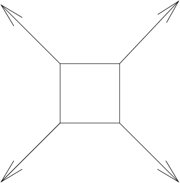

We now need to choose the multisets , , and . First we pick subsets of :
We then modify the ’s to produce the ’s. Specifically, we must multiply one of the members of by . We obtain
This is the stage in the process where we would perturb the ’s to produce the ’s. However, we got lucky this time – we already have for , , so no perturbation is necessary and we just take . So we take the curve to be and we take the map to be given by or, to be completely explicit,
At this point, the reader may reasonably wonder how to extract an actual equation for the curve . This is basically a problem of implicitization, the recovery of the equation of an algebraic variety from a parametric representation, but it is worse than the usual implicitization problem because the parameterization is analytic, not algebraic. This problem deserves a great deal of study, which has been begun in [28] and [29]. We will describe here a straightforward, but unwieldly method. Let denote the complete fan whose rays point in directions , , and . Then, by Proposition 1.2, the closure of in is torically transverse and has cohomology class corresponding to the linear relation between the rays of . Thus, obeys an equation of the form , for some , , , and in . Here we have written the coordinates on as and . In order to find , , , and , expand the infinite products for and as Laurent series around , and compare the coefficients of for , , , , . Note that this will express , , , and in terms of infinite sums. There is no reason to expect a better result; our algorithm will usually produce curves defined by equations whose coefficients are not algebraic functions of .
8. Superabundant Curves
In this section, we prove Theorem 3.4, which we restate for the reader’s convenience.
Theorem 3.4.
Suppose that has characteristic zero.
Let be a zero tension curve of genus one and degree . Suppose also that is well spaced. Then there is a (punctured) genus one curve over , and a map so that .
See the end of Section 3 for the definition of “well spaced”.
For each nonnegative rational number , let be the subgraph of consisting of those points with distance less than or equal to from the circuit of . Let be the affine linear space spanned by . Then is an increasing chain of affine spaces which increases at a finite number of discrete indices. Let , , …, be the dimensions of the various ’s. Let be the value of at which the jump from to occurs and let , …, be the corresponding subgraphs of . We will also occasionally need to refer to the open subset of where we do not include those points at distance precisely from the circuit of ; we denote this by . Set . We can make a change of basis in such that is . By the arguments in the previous section, we can find , …, , multisubsets of , and with equal to the length of the loop of such that . We can use the perturbation arguments of the preceding section to arrange that for , …, . However, for , all we can conclude is that . The strategy of our proof will be to show, by induction on , that we can arrange for the equality to hold for .
So, suppose that we have , …, and such that and such that holds for . We introduce the notation for the group of units of such that .
Lemma 8.1.
For each between and , the ratio is in .
Proof.
For , we have , which is in . So fix . Let , …, be the components of . We note that, for each , we have . This is because, by the zero tension condition, is the component of the edge of pointing inward from . Since this is an edge of , that component is zero. So we can pair of the elements of with those of . In each pair , we have which is by Proposition 4.2. Then is a product of ratios which are in and hence is itself in as we claimed. ∎
We introduce the notation for , which we have just shown to be in . When , then is simply .
Lemma 8.2.
The abelian group is divisible.
Proof.
This is where we will use that has characteristic zero, and hence that for every nonzero integer . Let and let be a nonzero integer. Then, since is algebraically closed, has an root in , and even has a root which lies in and reduces to in . (Proof – let , …, be the roots of in . Since , we know that all of the are in . Let be the reduction of in . Then we have in so, by unique factorization in , one of the reduces to in .) So, let , with . Then where . As , we have so and we deduce that so is in as desired. ∎
Let , …, be the edges of which are not in , but which have endpoints that are in . Let , …, be the slopes of these edges, directed away from .
Lemma 8.3.
There exist scalars , …, such that and such that, if and are distinct edges with the same endpoint, then .
Proof.
Let be the image of in . We first show that we can find , …, obeying the required inequalities with . Let be the space of -tuples of rational numbers such that . We want to show that has a point not contained in any of the hyperplanes , where ranges over pairs of indices such that and share an endpoint. Since is a linear space, we just need to show that is not contained in any of these hyperplanes.
Let and share the endpoint , which is necessarily a boundary vertex of . Suppose, for the sake of contradiction that is contained in the hyperplane . Then in particular, does not contain any point with and . This means that is not in the span of
Equivalently, is not in . Let be a hyperplane in which contains and does not contain . Then is at distance from the loop of , while every other boundary vertex of is farther away, contradicting our hypothesis that is well spaced.
So, now we have obeying the required inequalities with in . Let , …, be the boundary vertices of and let be the slope of the edge of pointing inward from . Then, by Lemma 5.1, the span . Let . Now, by the zero tension condition, . So we have . We regroup this expression and take the coefficient of to be our . If and share the endpoint then the coefficients of and in this expression are and . Since , we also have and we have achieved the goal.
∎
Our strategy will be to choose , … and, for each , multiply those elements of which lie in the component of containing by . This will have the effect of multiplying by where . We need to achieve two things – we must make the new values of be for and we must not change the fact that .
Now, by lemma 5.1 applied to for some small , we know that the span . Since is a divisible group, this means that we can arrange to make assume any value that we want for and in particular, we can make . The trouble is that we might no longer have . Now, multiplication by an element of will fix all of the points of and will move each component of by an isomorphism. Our only fear is that two of these components which are connected to at the same vertex, say , will swing so that the edges at which they attach to , say and , overlap for some length.
Let be the vector found in Lemma 8.3. Assume that we have arranged for to be for , , …, . Now consider choosing some and, for each , further multiplying those elements of which lie in the component of containing by . This will multiply by , so this will not break our achievement of making the (for , …, .) Also, if and share an end point , then the components of containing and will be multiplied by and respectively, two different scalars, and so, for generic , they will not overlap.
We have now completed the inductive step, showing how to make equal to for . Continuing in this manner, we will eventually have all the equal to , and thus the map will be well defined. At that point, we will have a curve and a map with as desired.
9. The necessity of well-spacedness and the -invariant
We have been studying genus curves over by identifying them with Tate curves. It is therefore natural to ask to what extent we may assume that a genus one curve over is a Tate curve.
Theorem 9.1.
Let be a genus one curve over and its projective completion. Let be the -invariant of . Let be the extension of to a (flat, projective) family of stable curves with marked points over . (There is no need to take a branched cover of because is algebraically closed.)88 8 More precisely, after taking a finite base extension of , we may assume that is defined over . Since is noetherian, after another finite base extension, we may complete to a family of stable curves over . Then go back to , which was all we ever actually cared about. Then the following are equivalent:
- (1)
can be expressed as a Tate curve for some with .
- (2)
.
- (3)
The fiber of over is a union of genus zero curves.
Moreover, if these equivalent conditions hold, we have .
Proof.
The equivalence of (1) and (2) is [20, Section 3, Statement VIIIa]. (Observe that Roquette’s conditions (i) and (iii) are automatic when is algebraically closed, the latter because the Hasse invariant lives in the group which is trivial for algebraically closed.) If is the number of points in , then gives a map from to the moduli space of stable genus 1 curves with marked points. Forgetting all but one of the points, we get a map to the moduli space of stable genus 1 curves with one marked point. This moduli space is a copy of the projective line, commonly known as the -line. Condition (3) is equivalent to saying that this map sends to the point at infinity on the -line, which is exactly what condition (2) says. We have because where each is an integer and hence has nonnegative valuation. ∎
Combining the above with Corollary 10.18, we see that if is trivalent and has first Betti number one then is a Tate curve. In this case, we can show that the condition that be well spaced is necessary, and that the length of the loop of is necessarily . Recall that every nonzero meromorphic function on a Tate curve is of the form for some and with .
Proposition 9.2.
Let be a trivalent tropical curve of genus and a zero tension curve parameterizing , with and injective on . Then the length of the loop of is , where is the -invariant of . Now suppose that has characteristic zero. Then is well spaced.
The idea that the length of the circuit of is the tropical analogue of the -invariant was suggested in [15] and pursued in [12]. E. Katz and H. and T. Markwig, have proven that the length of the circuit of is the -invariant of a trivalent curve for tropicalizations of cubic curves in .
Proof.
Our hypotheses are enough to ensure that is a Tate curve for some and that the map is given by for some , …, .
By our combinatorial construction of , the length of the loop of is . Lemma 5.2 ensures that is injective and thus the loop of and the loop of have the same length.
Now, assume that has characteristic zero and (for the sake of contradiction) that is not well-spaced. After a change of coordinates, we may assume that is the coordinate hyperplane. Assume for the sake of contradiction that is the boundary vertex of which is closest to the loop of and let denote the distance from to the loop of . Then is trivalent by hypothesis. One of the edges of is between and the loop of , this edge is contained in so its component is . Let the components of the other two edges be and for some positive integer . Let and be the elements of and respectively which are beyond these edges. Then, we have for any indices and from to and similarly . On the other hand, . So,
for some with and thus . We have used that has characteristic zero to deduce that, if then .
Pair off the elements of with elements of that lie in the same component of , this is possible by the same argument as in the proof of Lemma 8.1. We write the pairs as for . Then in each pair , we have . But we are supposed to have , so . Then the left hand side differs from by an element of valuation while the right hand side differs from by an element of valuation greater than , a contradiction. ∎
10. Appendix: Tropical Generalities and Theorem 3.1
In this appendix, we describe some general tropical constructions. Our eventual aim is to explain and prove Theorem 3.1 in the case where is a curve such that is reduced for every vertex of . In this section we will prove many theorems for tropical varieties in general and then apply them to the case of curves. For clarity, we use for a variety which may have any dimension and for a curve. We restate our goal for the reader’s convenience.
Theorem 3.1 – Reduced Case.
Let be a connected (punctured) curve of genus over equipped with a map . Let be the degree of . Suppose that is reduced for every vertex of . Then there is a connected zero tension curve of degree and genus at most with .
If there is some vertex of for which is not rational, then we can take .
We begin by discussing the local geometry of .
Proposition 10.1.
Let and let . Then the star of at is .
Proof.
The next result roughly states that, when is a pretty general point of then is very symmetric. For any polytope in , let denote the linear space spanned by vectors of the form for , . If is defined by inequalities of the form for various , then there is a subtorus which has dimension . The torus is cut out by the equations where ranges over those elements of such that is constant on .
Proposition 10.2.
Let be a face of a good subdivision of . Then, for in the relative interior of , the variety is invariant under the action on of the torus .
Proof.
By proposition 2.1, for , we have . But is clearly invariant under , as, for any , the polynomial is homogenous with respect to the grading by . ∎
Note that this has an immediate corollary:
Corollary 10.3.
The dimension of is less than or equal to that of .
Proof.
Let and suppose for the sake of contradiction that . Then there must exist a face of with dimension . Let lie in the relative interior of . By description (5) of in proposition 2.2, is not empty. Thus, since acts freely on , we have . But is a flat degeneration of , so its dimension can be no more than , a contradiction. ∎
Let be a face of a good subdivision of and let lie in the relative interior of . Set . Then splits (noncanonically) as and we have and . We have . When is pure of dimension , this allows us to improve Corollary 10.3.
Proposition 10.4.
If is integral and -dimensional then, for any , is pure of dimension . As a corollary, if is any face of a good subdivision of then .
Note that “pure of dimension ” means that every irreducible component of a scheme has dimension , but it permits that there may be associated primes of smaller dimension.
Proof.
After taking a finite extension of , we may assume that and for some . Recall our description of as the fiber over of . Now, is integral because it is the Zariski closure of an integral variety. (A subring of a domain is a domain.) Taking the closure increases the dimension by one. Taking the quotient by brings the dimension back down to again, as in a domain any single non-zero element is a regular sequence. So the fiber of over is -dimensional again. ∎
In particular, suppose that is pure of dimension and is a -dimensional face of a good subdivision of . Then is -dimensional and thus has finite length. Let be the length of . Note that we now know, if is a curve in , that is pure of dimension . In other words, is a graph in this case.
We now prove a result which shows, in particular, that if is a curve then is a zero tension curve.
Let be a finite rational polyhedral complex, pure of dimension , with a positive integer assigned to each maximal face of . Let be a -dimensional face of and let , …, be the collection of -dimensional faces of which contain . Then is a lattice of dimension and the image of is a ray in this lattice. Let be the minimal lattice vector along this ray. We say that the zero tension condition holds at if . We say that is a zero tension complex if the zero tension condition holds at every -dimensional face of . Note that, if is a subdivision of and we define to be where is a -dimensional face of and is the face of containing , then is a zero tension complex if and only if is. We will now show that tropical varieties are zero tension complexes. We first tackle the case of a curve with constant coefficients.
Proposition 10.5.
Let be an algebraic curve. Let be the degree of ; write as where is a positive integer and a primitive lattice vector of . Then the rays of are precisely in the directions , …, and the sum of the multiplicities of the rays in direction is . As a corollary, .
Proof.
Let be the projective completion of the normalization of and the rational map with image . Let be a primitive lattice vector. We will show that, first, if and only if there there is a multiple of in the degree of and, second, that has the same multiplicity in both cases.
Without loss of generality, we can choose coordinates such that and . Then we can embed into . Let be the subset of on which can be extended to a map to and write for the extended map. The closure of in is . We claim that we have the equality
| (3) |
of subschemes of . To see this, let be a polynomial in . We must show that vanishes on the left hand scheme if and only if it vanishes on the right hand scheme. Note that both sides are clearly homogenous in the coordinate, so we may assume that is homogenous in . Since is a unit in , we may furthermore assume that does not occur in at all.
Let be the ideal defining . Now, since is homogenous in the -grading, the condition that vanishes on the left hand scheme is that there be a with . If such a exists, it is of the form . In particular, is in the coordinate ring of and hence vanishes on the closure of in , which is . But then, as , we have that vanishes on . This chain of reasoning can easily be reversed. So the same polynomials vanish on the schemes on each side of (3) and so (3) is established.
Now, by definition, is in if and only if the left side of (3) is nonempty. So is in if and only if there is a point of on which is defined and such that is in . Now, is defined at a point of if and only if the rational functions on have no zeroes or poles at for , …, and has no pole at . Moreover, lands in if and only if is at . So we see that is in , if and only if the left hand side of (3) is nonempty, if and only if the right hand side of (3) is nonempty, if and only if there is a point in such that has neither a zero nor pole at for …, and has a zero there. But this last is precisely the definition of a multiple of being in the degree of . Moreover, if is as above, then the length of the scheme at is the order of vanishing of at ; this yields the equality of multiplicities.
It follows that , as we have now shown that the are the degree of a curve. ∎
We have just shown that, for a curve with constant coefficients the unbounded rays of correspond to the degree of . In fact this is true for curves that do not have constant coefficients; we leave the details to the reader.
Proposition 10.6.
Let be an algebraic curve. Let be the degree of ; write as where is a positive integer and a primitive lattice vector of . Then the unbounded rays of are precisely in the directions , …, and the sum of the multiplicities of the rays in direction is .
So, if is a curve, then is a graph of the correct degree. We now finish proving that, if is a curve, then is a zero tension curve.
Proposition 10.7.
Let be pure of dimension . Fix any good subdivision of and define weights by the length of as described above. Then is a zero tension complex.
Proof.
Let be a face of of dimension . Let denote the star of at , then is invariant under translation by and . One can easily check that the multiplicities of rays of are the same as the multiplicities of the corresponding faces of . Thus, we are reduced to checking the claim for , which is purely one-dimensional and has constant coefficients.
We may thus switch notations, calling what used to be called by the name , and assume that is purely one-dimensional and has constant coefficients. If is reduced and irreducible, then we have already proven the result in the previous proposition. Unfortunately, the possibility that is not reduced leads to significant difficulties, to which we now turn.
Let , … be the irreducible components of and let be the multiplicity of . Let be the reduction of . Clearly, , since description (1) of in Theorem 2.2 only sees the structure of as a point set. We claim that, for spanning a ray of , the multiplicity of in is the sum, over the components of , of times the multiplicity of in .
As in the proof of Proposition 10.5, we may assume that . Set . Let be the closure of in and let be the closure of . Then the multiplicity of in is the length of the scheme theoretic intersection and the multiplicity of in is the length of . So we want to show that
We project onto the coordinate, giving a map . Since and are defined as the closures of varieties in , they do not have any associated primes over the point of . So and are flat over the point of and thus, for a generic , we have and the same applies to each . So we are reduced to proving
for a generic .
For a generic , will not contain any of the intersections of the , nor any embedded points of the , nor any components for which . For such an , is the disjoint union of the schemes and the length of is times the length of .
So, we have now shown that the rays of are precisely the rays that occur in and the multiplicity of a ray in is the sum (on ) of times that ray’s multiplicity in . Since each is a reduced curve, we know from Proposition 10.5 that the rays of each , counted with multiplicity, sum to zero. So the same holds for . ∎
We now know that, if is a curve, then is a zero tension curve of the correct degree. What remains is to show that the first betti number of is bounded by the genus of . Unfortunately, if we take the most obvious zero tension curve with , this may not be true. Consider the following example, which we discussed earlier as Example 6.5: take to be a power series field over . For simplicity, we take not to have characteristic or . We map to by the rational map
Let be the open subset of on which is defined. As we computed in Example 6.5, is as shown in Figure 3. Let us check directly that the point is in . Suppose that , where and the ellipsis represents an element of valuation higher than the displayed leading term. Then . Similarly, if with , then . So the points of that are of the form or have valuation . All points of with valuation are of one of these forms, as can be verified using the techniques of Section 6. This shows that, as a point set, . In fact, this is an equality of schemes.
Note, in particular, that is disconnected. Intuitively, it seems that passes through itself at and should really be thought of as a tree which just happens to pass by itself at that point. It turns out that the two components of correspond to the two branches of passing through . We can modify this example by making the third coordinate , giving the map also discussed in Example 6.5. Then is the same as before, but is now two crossed lines with an embedded point at the crossing. (In other words, the ideal of is .) So we see that, while the disconnected nature of is related to our problems, it is possible to have this difficulty in a case where the initial scheme is connected.
Despite examples such as the above, it is true that we can always find a zero tension curve with and . We give a slightly more precise statement.
Theorem 10.8.
Continue the above notations and , in particular continue the assumption that is reduced for every vertex of . Then there is a zero tension curve with connected and the genus of less than or equal to the genus of , such that . Moreover, if is any edge of (a good subdivision of) , we have .
In order to prove Theorem 10.8, we will need two constructions. The first is a construction which, given a polyhedral complex, builds a family over whose generic fiber is a toric variety and whose special fiber is a union of toric varieties. The second is a construction which allows us to build a single family over whose general fiber is and whose special fiber contains every , as ranges over . This is a generalization of a construction of Tevelev in [30].
Let be a finite subset of , with cardinality . Then there is a map given by . Let be the convex hull of . Define the semigroup by , then we write where the grading on is by the last coordinate. At times we will need to record the dependence of on the field , at which point we will write . We can also describe as the toric variety associated to the normal fan of . The following result is well known.
Proposition 10.9.
The map extends to a map from to . The image of this map is the Zariski closure of .
We will need to have a generalization of this result that works in families over . Let be a finite subset of and let , …, . Then there is a map by . We will now define a variety over which allows us to extend in a manner similar to that in which allows us to extend .
Let denote the convex hull of . Let be the function defined as follows: , where the supremum is taken over all affine linear functions such that for , …, . The function is piecewise linear and its domains of linearity are polytopes which are convex hulls of subsets of . Let , …, be the domains of linearity of , then is called the regular subdivision of induced by . We denote this subdivision by . By taking a branched cover of , we may assume that, on each , the slope of is in . When this occurs, we will say that is integral.
Let be the semigroup ring associated to the semigroup . We write elements of as where is in and and are in and respectively. Here is a formal symbol where . Let be the subring of consisting of those sums where and . Clearly, is an -algebra, and inherits a grading by . Let .
Proposition 10.10.
Suppose that is integral. We have the following consequences: The variety is flat and projective over . The fiber of over is . The fiber of over is a union of the toric varieties , glued according to the overlaps between the . There is a map which extends .
Here is .
Proof.
Clearly, is a torsion free -module, and hence flat over . Also, is finitely generated as an -algebra, with generators of positive degree, so the map is projective. The fiber of over is and consists of those sums where and is any element of . This is precisely .
Now, let us consider . As an additive group, we see that is a vector space with basis , where ranges over pairs with .99 9 This is where we need the slopes of to be in , otherwise might not be an integer. The multiplicative structure of is that if and otherwise. In other words, if the convex function is linear on the line segment connecting to . So is isomorphic to the subring of where, if is in both and then we require that have the same coefficient in and in . Now, is and imposing the stated conditions on the coefficients of the precisely glues these toric varieties together.
Finally, we want to describe the map . We know that . We map to by sending to . Let be the ideal of generated by as runs from to ; this is the preimage of the irrelevant ideal of . In order to show that this gives a map we just have to check that the radical of is the irrelevant ideal of . Clearly, is homogenous for the grading of by , so it is enough to check that, for any monomial which is in the irrelevant ideal of , some power of is in . The condition that be in the irrelevant ideal of is simply that is positive.
So, consider some monomial of with . Then and . Let be the domain of linearity for in which falls. Let , …, be the vertices of . Then for , …, . Since is in the convex hull of the , we can write as where are nonnegative rational numbers with . Since is linear on , we have . Clearing out denominators, we can find nonnegative integers with , and . We may also assume that divides . Then
So we see that is in the radical of . But so is in the -module generated by the radical of and is, hence, in the radical of itself.
We now have shown that there is a well defined map . The torus is canonically an open subvariety of and hence an open subvariety of . Explicitly, corresponds to the localization of . The map is given by , which precisely corresponds to . ∎
Remark: There are two variants of this construction which have been previously published. Firstly, one may consider the limit inside of the image of . As a point set, this limit is a union of toric varieties, but it can have a quite sophisticated nonreduced structure, see [27]. By contrast, after a base extension to ensure that is integral, the fiber of over is always reduced, but the map from this fiber to may fail to be a closed immersion. Secondly, just as toric varieties can be described by fans rather than by polytopes, there is a description of this construction in terms of fans in [18]. Our approach may be thought of as an intermediate ground between these approaches, which keeps the map to projective space available but retains the reduced varieties of the more abstract version.
Proposition 10.11.
Let . Extend if necessary so that is a point of and is integral. Let be the face of the regular decomposition of on which is minimized. Then the limit in of is in the interior of the stratum of .
Proof.
Let be the minimum value of as ranges through . The embedding of the point into corresponds to the map of graded rings by . If we rescale the -th graded component of by for some , we get the same map . We rescale by , so that our map is now . Since implies that , this map extends to a map . We claim this gives us a map . Once we know this, the image of will be the limit of .
Our fear is that the preimage of under might be the irrelevant ideal. Now, is spanned by the images of . We write for the image in of . We see that maps to in if and only if , in other words, if and only if . So we see that the preimage of is not the irrelevant ideal, as it does not contain for .
Moreover, we see that the map factors through the subvariety but not through for any proper face of , so we get that lands in the interior of . ∎
Now, let be a subvariety of . Choose an isomorphism of with , and hence an embedding of into . We will therefore feel free to write in place of . Let be the closure of in . Then we have an embedding of into the Hilbert scheme by . Let be the closure of in under that map.1010 10 Here is the scheme over equipped with a universal closed subscheme of so that, for every scheme with a map , every closed subscheme of which is flat over is pulled back in a unique manner from along a map .
Proposition 10.12.
There is a projective embedding of , for some , and a set and some scalars , …, such that the restriction to of is .
Proof.
This proof amounts to unraveling the proof that is projective. Let denote the Hilbert polynomial of . By a result of Gotzmann [9], there is a positive integer such that, if is any subscheme of which is flat over with hilbert polynomial , then is determined by the degree terms of its defining ideal and has codimension for every such . Then we get a projective embedding of the component of containing by first mapping to the point of the Grassmannian and then embedding this Grassmannian into projective space by the Plücker embedding. We need to be a bit more specific: we take coordinates on to be the obvious coordinates , with and use the obvious Plücker coordinates on the Grassmannian. Let be the set of indices for which . Every Plücker coordinate not indexed by is on , so is embedded into by the Plücker coordinates , . We call this map .
Now, it is easy to check that the action of on rescales the Plücker coordinates by a character of . So the map , restricted to is of the form for some characters of and some elements . Rescaling our target by an element of , we can assume that is of the form for some . This is the required claim. ∎
We continue to let be a subvariety of , which we view as embedded in . Let be as in the preceding proposition, let be the convex hull of , let be as before and let be the regular subdivision of obtained from . Extend if necessary so that is integral. Let be the closure of in . We’ll write for the fiber of over and for the fiber of over . Clearly, is a compactification of over and is a flat degeneration of .
Proposition 10.13.
Let be a face of . Let be such that the function is minimized precisely on ; extend if necessary so that . Let be the linear space spanned by , for and . Let be the orthogonal space to and let be the connected subtorus of associated to .
Then is invariant under and the intersection of with the interior of is .
This proof is closely modeled on an argument of Tevelev, see [30].
Proof.
By our construction of , there is a map . Let be the pull back to of the universal family over and let be the intersection of with the open torus in . We will write for the torus bundle over in which lives. Let be the section of given by the point in each fiber. (Note that this fiber is sometimes and sometimes .) As in [30], we see that the closure of in is the projection to of .
Consider as a point in . Let be the limit of over the zero fiber of . (I.e. take the Zariski closure of the point in and intersect it with the zero fiber.) The fiber of over is . By Proposition 10.11, is in the interior of .
Now, let us consider what , and look like over the interior of . All statements in this paragraph are implicitly limited to the parts of our families that live over the interior of . The interior of is the torus . The torus bundle is isomorphic to . The torus acts on this product by multiplication by , and is taken to itself under this action. Thus, in particular, each fiber of is preserved by . We have seen in the preceding paragraph that the fiber of over is , so we see that is preserved by . Moreover, since this torus action takes to itself, we see that, identifying with , the part of over the interior of is where is the class of in . So is and the projection of onto the interior of is as desired. ∎
Corollary 10.14.
Let be the polyhedral subdivision of for which and are in the relative interior of the same face if and are minimized on the same face of . Then is supported on a subcomplex of and the induced subdivision of is a good subdivision.
We will write for the subcomplex of containing .
Proof.
We showed that depends only on the face of in whose relative interior lies. Now, if and only if is empty. So is supported on a subcomplex of . The fact that is constant on the relative interiors of the faces of is the definition of a good subdivision. ∎
We may hence use our notation , where is a face of . We summarize our accomplishments:
Proposition 10.15.
Let be a subvariety of . Then, after possibly taking a branched cover of , there is a compactification of (over ), a flat projective degeneration (over ) of to a variety (over ) and a good subdivision of such that , with the disjoint inside and in the closure of only if .
We are now closing in on the proof of Theorem 10.8, in the case where is reduced for every vertex of . Let be the degeneration of described above. The idea is that, since is a degeneration of a genus curve, its components can’t form a graph of first betti number more than . We have built so that the structure of more or less captures the structure of the components of . There are two main things that can go wrong. First, if is a vertex of , it is possible that is disconnected and should thus correspond to multiple vertices of . We will deal with this by defining our graph appropriately. Secondly, if is an edge of , we might worry that the local structure of near looks like two crossing lines with some extra non-reduced structure at the crossing point, in which case it shouldn’t correspond to an edge of . To deal with the latter obstacle, we need the following lemma. The proof was suggested to me by Paul Hacking.
Lemma 10.16.
Let , , and continue to have the above meanings. For a face of , let be the scheme theoretic closure of . Then the complex of sheaves
is exact. Here the maps are the obvious restriction maps from to whenever is a facet of , sign twisted in the usual fashion.
Proof.
Recall our notation for the toric degeneration in which sits. Let be the fiber of over and let be the closed face of associated to the face of . Then the complex of sheaves
is easily exact. Recall the notations , and from the proof of Proposition 10.13., and write for the projection . Let denote the portion of lying over . Then is flat over (it is pulled back from the universal family over the Hilbert scheme) so the complex
is exact. But is transverse to inside , so the corresponding complex with replaced by is exact. As shown in the proof of Proposition 10.13, projects down isomorphically to . We claim that, similarly, projects down isomorphically to , so the complexes and are the same. Since and is closed, we know that . We want to show that if, on some open set , a function vanishes on then it vanishes on .
Write for the part of over the interior of . Since is flat over , we know that, as schemes, is the closure of . By the transversality result, is the closure of . With and as in the previous paragraph, since is an isomorphism, we know that vanishes on . Then also vanishes on and hence, using that is an isomorphism once more, vanishes on . ∎
We also need the following lemma:
Proposition 10.17.
In the above notation, assume that is reduced. Then is also reduced.
Proof.
In general, if is an open subscheme of some variety , and is a closed subscheme of , then is reduced. This is a local fact, so we can check the corresponding affine property: Let be a ring, a multiplicative subset of , and a domain with a surjection. Then we are to show that the pullback of to is a prime ideal or, in other words, the image of under is a domain. A subring of a domain is always a domain. ∎
Now, finally, we can prove Theorem 10.8.
Proof of Theorem 10.8.
Let be a curve in and let, , and be as above. Then is one dimensional. inherits the structure of a one dimensional polyhedral complex, that is to say, a graph, from . Define a graph as follows: for each vertex of , let , …, be the connected components of the closure of . There will be a vertex of for each , as ranges over all the vertices of .
Now, consider any edge of . Let , …, be the connected components of . If for some then we must have , i.e., must be one of the two end points of . Moreover, if is one of the endpoints of , then there is clearly at most one such that because we defined to be the connected components of . In fact, we claim that there is such a . Let be the direction of the edge pointing away from , then . So every point of is the limit of some path in . There is an edge of for each connected component of a , as ranges over the edges of . This edge is denoted . The endpoints of the edge are and where and are the endpoints of and is the connected component of containing .
We now define the weighting on the edges of . The edge is given weight , the length of the zero dimensional scheme . Next, we describe the map from to . We map to and we map to .
It is transparent that is the image of . The condition on weights holds because . The zero tension condition holds at vertices of because, for every vertex , is simply given by the rays in the direction of for those edges such that is in , so the zero tension condition for holds by the zero tension condition applied to the .
Finally, (using Proposition 10.17), each is a reduced, connected, projective curve. So the holomorphic Euler characteristic of each is at most . On the other hand, each is zero dimensional. So the holomorphic Euler characteristic of each is at least . Now, by Proposition 10.16, . So is at most the difference between the number of vertices of and the number of edges, i.e., the Euler characteristic of . But is a flat degeneration of , which is a curve of genus , so . We deduce that and hence is at most . If any of the components is not rational, then is strictly less then . ∎
We see that, if any of the components of are not rational, or if any of them meet along singularities other than nodes, we can take to have first Betti number less than . A similar situation occurs for the zero tension curve constructed in the proof of Siebert and Nishinou, where is replaced by the stable limit of . We would like to use this observation to prove that the stable limit of consists only of rational components in certain cases. Unfortunately, it is possible that does not have this form but that there is some other for which . However, when is trivalent, we can rule this possibility out.
Corollary 10.18.
Suppose that is trivalent and that is a zero tension curve with , with injective and such that the genus of is equal to . Let be the projective curve (over ) containing and let .
Consider as a stable curve over with marked points and (taking a branched cover if necessary) extend to a flat, proper family over , of stable curves with marked points. The zero fiber of this family is a union of genus zero curves.
Proof.
If not, then there is some other zero tension curve for with , as discussed above. But then, by Lemma 5.2, we may make injective by restricting to a subgraph of ; this can only lower . So we may assume that , like is injective, and thus . But , a contradiction. ∎
References
- [1] R. Bieri and J.R.J. Groves: “The geometry of the set of characters induced by valuations” J. reine und angewandte Mathematik 347 (1984) 168–195.
- [2] T. Bogart, A. Jensen, D. Speyer, B. Sturmfels and R. Thomas: “Computing Tropical Varieties” Journal of Symbolic Computation 42, no. 1-2 (2007) 54–73.
- [3] M. Einsiedler, M. Kapranov and D. Lind: “Non-Archimedean amoebas and tropical varieties”, J. reine und angewandte Mathematik 601 (2006) 139–157.
- [4] D. Eisenbud: Commutative Algebra with a View Toward Algebraic Geometry Springer-Verlag 1995
- [5] W. Fulton, Introduction to Toric Varieties Princeton University Press (1993)
- [6] W. Fulton and B. Sturmfels: “Intersection theory on toric varieties” Topology 36 (1997), no. 2, 335–353
- [7] A. Gathmann, M. Kerber and H. Markwig, “Tropical fans and the moduli spaces of tropical curves” arXiv:arXiv:0708.2268
- [8] A. Gathmann and H. Markwig, “The Caporaso-Harris formula and plane relative Gromov-Witten invariants in tropical geometry” Math. Ann. 338 (2007), 845–868
- [9] G. Gotzmann: “Eine Bedingung für die Flachheit und das Hilbertpolynom eines graduierten Ringes” Mathematische Zeitschrift 158 (1978) 61–70
- [10] M. Kalkbrener and B. Sturmfels: “Initial Complexes of Prime Ideals” Advances in Mathematics 116 (1995) no.2 365–376
- [11] E. Katz, M. Kerber and H. Markwig: “The -invariant of a plane tropical cubic” Preprint arXiv:math/0709.3785
- [12] M. Kerber and H. Markwig: “Counting tropical elliptic plane curves with fixed -invariant” Preprint arXiv:math/0608472
- [13] D. Maclagan, “Antichains of Monomial Ideals are Finite” Proceedings of the American Mathematical Society 129 (2001) 1609–1615
- [14] G. Mikhalkin, “Enumerative Tropical Geometry in ” JAMS, to appear arXiv:math.AG/0312530
- [15] G. Mikhalkin, “Tropical Geometry and its Applications”, Proceedings of the ICM 2006 Madrid, Spain, 827-852
- [16] G. Mikhalkin, “moduli spaces of rational tropical curves”, to appear in the proceedings of the 2006 Gökova Geometry-Topology Conference. http://arxiv.org/abs/0704.0839
- [17] J. Morgan and P. Shalen: “Valuations, trees, and degenerations of hyperbolic structures I” Ann. of Math. (2) 120 (1984) no. 3 401–476
- [18] T. Nishinou and B. Siebert: “Toric degenerations of toric varieties and tropical curves” arXiv:math.AG/0409060
- [19] S. Payne, “Fibers of Tropicalization”, arXiv:0705.1732
- [20] P. Roquette Analytic theory of elliptic functions over local fields Vandenhoeck and Ruprecht 1970
- [21] Shustin, E. and Tyomkin, I. “Patchworking singular algebraic curves. I.” Israel J. Math. 151 (2006), 125–144.
- [22] J. Silverman: Advanced topics in the theory of elliptic curves Grad. Texts in Math. vol. 151, Springer-Verlag 1994
- [23] D. Speyer “Tropical Geometry”, PhD thesis, UC Berkeley, 2005
- [24] D. Speyer and B. Sturmrfels, “The Tropical Grassmannian”, Adv. Geom. 4 (2004), no. 3, 389–411.
- [25] B. Sturmfels: Gröbner Bases and Convex Polytopes, University Lecture Series 8, American Mathematical Society, 1996
- [26] B. Sturmfels: Solving Systems of Polynomial Equations Amer.Math.Soc., CBMS Regional Conferences Series, No 97 (2002)
- [27] B. Sturmfels: “Gröbner bases of toric varieties” Tohoku Math. J. (2) 43 (1991), no. 2, 249–261.
- [28] B. Sturmfels and J. Yu: “Tropical Implicitization and Mixed Fiber Polytopes” preprint arxiv:0706.0564
- [29] B. Sturmfels, J. Tevelev and J. Yu: “The Newton Polytope of the Implicit Equation” preprint arXiv:math/0607368
- [30] J. Tevelev: “Compactifications of Subvarieties of Tori”, Amer. J. Math 129 no. 4 (2007)
- [31] G. Ziegler: Lectures on Polytopes Graduate Texts in Mathematics vol. 152, Springer-Verlag: New York 1995