Observability of the virialization phase of spheroidal galaxies with radio arrays–2007
Abstract
In the standard galaxy formation scenario plasma clouds with a high thermal energy content must exist at high redshifts since the proto-galactic gas is shock heated to the virial temperature, and extensive cooling, leading to efficient star formation, must await the collapse of massive halos (as indicated by the massive body of evidence, referred to as downsizing). Massive plasma clouds are potentially observable through the thermal and kinetic Sunyaev-Zel’dovich effects and their free-free emission. We find that the detection of substantial numbers of galaxy-scale thermal SZ signals is achievable by blind surveys with next generation radio telescope arrays such as EVLA, ALMA and SKA. This population is even detectable with the 10% SKA, and wide field of view options at high frequency on any of these arrays would greatly increase survey speed. An analysis of confusion effects and of the contamination by radio and dust emissions shows that the optimal frequencies are those in the range 10–35 GHz. Predictions for the redshift distributions of detected sources are also worked out.
Keywords:
galaxies: formation – galaxies: high-redshift – instrumentation: interferometers1 Introduction
A satisfactory theory of galaxy formation requires a good understanding of the complex physical processes governing the collapse of primordial density perturbations and the early galaxy evolution. Measurements of the galaxy luminosity and stellar-mass functions up to substantial redshifts have highlighted that these functions show conspicuous differences with respect to the halo mass functions predicted by the cold dark matter (CDM) theory with the ”concordance” cosmological parameters. At the low-mass end, the halo mass functions is much steeper than the galaxy luminosity function. As discussed by many authors (Larson 1974: Dekel & Silk 1986; Cole 1991; White & Frenk 1991; Lacey & Silk 1991; Kauffmann et al. 1993; Cole et al. 1994; Somerville & Primack 1999; Granato et al. 2001; Benson et al. 2003), the relative paucity of low-luminosity galaxies may be attributed to the quenching of star formation in low-mass halos by energy injections from supernovae and stellar winds, and by photoionization of the pre-galactic gas. This leads to the conclusion that efficient star formation must await the collapse of massive halos. On the other hand, the above processes have little effect on very massive halos, which, in the absence of additional relieving mechanisms, would convert too large fractions of gas into stars, yielding too many bright galaxies, with wrong metallicities (Thomas et al. 2002; see Benson et al. 2003 and Cirasuolo et al. 2005 for discussions of the effect of quenching mechanisms). An effective cure for that is the feedback from active nuclei (AGNs), growing at the galaxy centers (Granato et al. 2001, 2004; Bower et al. 2006; Croton et al. 2006)11 1 Note that the AGN feedback invoked by Granato et al. is radically different from that advocated by Bower et al. and Croton et al.. The former is a property of all AGNs and is attributed to a combination of radiation pressure (especially line acceleration) and gas pressure. The latter is associated to the radio active phase of quasars (‘radio mode’ feedback)..
During their very early evolutionary phases, massive proto-galaxies are expected to contain large amounts of hot gas, but the gas thermal history is obscure. According to the standard scenario (Rees & Ostriker 1977; White & Rees 1978), the proto-galactic gas is shock heated to the virial temperature, but this view has been questioned (Katz et al. 2002; Binney 2004; Birnboim & Dekel 2003; Kereš et al. 2005), on the basis of independent approaches: analytic methods, a high-resolution one-dimensional code, smoothed particle hydrodynamics simulations. The general conclusion is that only a fraction, increasing with halo mass, of the gas heats to the virial temperature. The hot gas is further heated by supernova explosions and by the AGN feedback, and may eventually be pushed out of the halo. Kereš et al. (2005) and Dekel & Birnboim (2006) find that there is a critical shock heating halo mass of , above which most of the gas is heated to the virial temperature, while most of the gas accreted by less massive halos is cooler.
The large thermal energy content of the hot proto-galactic gas in massive halos makes this crucial evolutionary phase potentially observable by the next generation of astronomical instruments through its free-free emission and the thermal and kinetic Sunyaev-Zel’dovich effects (Oh 1999; Majumdar, Nath, & Chiba 2001; Platania et al. 2002; Oh, Cooray, & Kamionkowski 2003; Rosa-González et al. 2004; De Zotti et al. 2004). In this paper we investigate the detectability of this proto-galactic gas exploiting an up to date model. For the purposes of the present analysis, the adopted model can be taken as representative of the most popular semi-analytic models (White & Frenk 1991; Kauffmann et al. 1993; Cole et al. 1994; Somerville & Primack 1999; Benson et al. 2003), that all adopt a similar mass function of dark matter halos, a cosmological gas to dark matter ratio at virialization, and assume that all the gas is heated to the virial temperature.
Even if some single dish telescopes have the required theoretical sensitivity, especially at mm and sub-mm wavelengths (e.g. LMT/GTM, GBT at 3 mm, Rosa-González et al. 2004) these continuum observations will be hampered by fluctuations in tropospheric emission. Interferometric array observations offer a better trade off between angular resolution, sensitivity and control of systematics (Birkinshaw & Lancaster 2005) together with larger fields of view, and allow us to work at lower frequencies where the sources of contaminations from backgrounds and foregrounds are lower and may be better estimated. For this reason we focus mainly on the capabilities of next generation interferometers: the Square Kilometer Array (SKA)22 2 http://www.skatelescope.org/, the Atacama Large Millimiter Array (ALMA)33 3 http://www.alma.info/, the Expanded Very Large Array (EVLA)44 4 http://www.aoc.nrao.edu/evla/, the new 7 mm capability of the Australia Telescope Compact Array (ATCA). We note that the situation for galaxy scale SZ detection is quite different from that for cluster SZ detection. Cluster SZ signals are stronger and have much larger angular scales than optimum for the interferometer arrays and are best observed with single dishes at high quality sites (Carlstrom, Holder & Reese 2002).
The outline of the paper is the following: in 2 we briefly describe our reference model; in 3, we present our predictions for the counts of proto-galaxies seen through their free-free emission and their thermal and kinetic Sunyaev-Zel’dovich effects; in 4 we analyze the potential of the next generation interferometers for detecting such signals, describe possible survey strategies, and discuss possible contaminating emissions and confusion effects; in 5, we summarize our main conclusions.
We adopt a -CDM cosmology with , , , , , consistent with the results from the Wilkinson Microwave Anisotropy Probe (WMAP) (Spergel et al. 2006).
2 Outline of the model
We adopt the semi-analytic model laid out in Granato et al. (2004), with the values of the parameters revised by Lapi et al. (2006) to satisfy the constraints set by the AGN luminosity functions. For the reader’s convenience, we summarize here its main features.
The model is built in the framework of the standard hierarchical clustering scenario, taking also into account the results by Wechsler et al. (2002), and Zhao et al. (2003a; 2003b), whose simulations have shown that the growth of a halo occurs in two different phases: a first regime of fast accretion in which the potential well is built up by the sudden mergers of many clumps with comparable masses; and a second regime of slow accretion in which mass is added in the outskirts of the halo, without affecting the central region where the galactic structure resides. This means that the halos harboring a massive galaxy, once created even at high redshift, are rarely destroyed. At low redshifts they are incorporated within groups and clusters of galaxies. Support to this view comes from studies of the mass structure of elliptical galaxies, which are found not to show strong signs of evolution since redshift (Koopmans et al. 2006). The halo formation rate at , when most massive early-type galaxies formed (Renzini 2006), is well approximated by the positive term in the cosmic time derivative of the cosmological mass function (e.g., Haehnelt & Rees 1993; Sasaki 1994).
We confine our analysis to galaxy halo masses between , close to the mass scale at the boundary between the blue (low mass, late type) and the red (massive, early type) galaxy sequences (Dekel & Birnboim 2006) and , the observational upper limit to halo masses associated to individual galaxies (Cirasuolo et al. 2005).
The complex physics of baryons is described by a set of equations summarized in the Appendix of Lapi et al. (2006). Briefly, the model assumes that during or soon after the formation of the host dark matter (DM) halo, the baryons falling into the newly created potential well are shock-heated to the virial temperature. The hot gas is (moderately) clumpy and cools quickly in the denser central regions, triggering a strong burst of star formation. The radiation drag due to starlight acts on the gas clouds, reducing their angular momentum. As a consequence, a fraction of the cool gas falls into a reservoir around the central supermassive black hole (BH), and eventually accretes onto it by viscous dissipation, powering the nuclear activity. The energy fed back to the gas by supernova (SN) explosions and AGN activity regulates the ongoing star formation and the BH growth. Eventually, the SN and the AGN feedbacks unbind most of the gas from the DM potential well. The evolution turns out to be faster in the more massive galaxies, where both the star formation and the BH activity come to an end on a shorter timescale, due to the QSO feedback whose kinetic power is proportional, according to the model, to .
Mao et al. (2007) found that, for the masses and redshifts of interest here, the evolution of the hot (virial temperature) gas mass, taking into account both heating and cooling processes, is well approximated by a simple exponential law
| (1) |
where is the gas mass at virialization, being the halo mass and the mean cosmological baryon to dark matter mass density ratio. The evolution timescale can be approximated as
| (2) |
The model proved to be remarkably successful in accounting for a broad variety of data, including epoch dependent luminosity functions and number counts in different bands of spheroidal galaxies and of AGNs, the local black hole mass function, metal abundances, fundamental plane relations and relationships between the black hole mass and properties of the host galaxies (Granato et al. 2004; Cirasuolo et al. 2005; Silva et al. 2004, 2005; Lapi et al. 2006).
2.1 The virial collapse
The virial temperature of a uniform spherically symmetric proto-galactic cloud with virial mass (dark matter plus baryons) and mean molecular weight , X and Y being the baryon mass fractions in the form of hydrogen and helium (we adopt X=0.75 and Y=0.25, no metals) is
| (3) |
where is the proton mass, G the gravitational constant, and the Boltzmann constant. The virial radius is given by
| (4) |
where is the mean matter density within
| (5) |
being the critical density. For a flat cosmology (), the virial overdensity can be approximated by (Bryan & Norman 1998; Bullock et al. 2001)
| (6) |
with , and
| (7) |
In the redshift range considered here (), we have
| (8) |
so that for the massive objects () we are dealing with, the only relevant cooling mechanism is free-free emission.
We assume that, after virialization, the protogalaxy has a NFW density profile (Navarro, Frenk & White 1997):
| (9) |
where ,
| (10) |
with
and (Zhao et al. 2003b; Cirasuolo et al. 2005).
2.2 The free-free emission
The free-free luminosity of the protogalaxy is computed integrating over its volume the emissivity given by (Rybicki & Lightman 1979):
| (11) | |||||
where the sum in the brackets is on all the chemical species in the gas (only H and He in our case) being the atomic number and and the number densities of electrons and of ions respectively, is the clumping factor, for which we adopt the value () given by Lapi et al. (2006), is the Planck constant and is the velocity averaged Gaunt factor. For the latter we adopted the analytical approximation formulae by Itoh et al. (2000) in their range of validity. Outside such range we used the formula given by Rybicki & Lightman (1979):
| (12) |
The gas density is assumed to be proportional to the mass density (). The electron number density is
| (13) |
being the proton mass. The adopted value of the clumping factor is assumed to be constant with radius, as in the model. This rather crude approximation stems from our ignorance of the complex structure of the gas distribution.
Finally, the flux scales with mass, redshift and frequency as
| (14) | |||||
where is the luminosity distance (Hogg 1999):
| (15) |
2.3 The thermal Sunyaev-Zel’dovich effects
The inverse Compton scattering of the Comic Microwave Background (CMB) photons by hot electrons produces a distortion of the CMB spectrum, known as Sunyaev-Zel’dovich (SZ) effect (Sunyaev & Zel’dovich 1972). The distortion consists in an increase of photon energies which implies a decrease of the CMB brightness temperature at low frequencies (GHz for K) and an increase at high frequencies:
| (16) |
where and is the comptonization parameter
| (17) |
being the Thomson cross–section and the electron mass. In the Rayleigh-Jeans region () eq. (16) simplifies to
| (18) |
The SZ signal corresponds to an unresolved flux
| (19) |
where
| (20) |
and is the surface integral of the comptonization parameter. scales with mass, redshift and frequency as
| (21) | |||||
and may be positive or negative depending on the sign of . Here we will quote only positive fluxes, taking the absolute value of .
For a virialized cloud with at , which has a virial temperature K, a mean electron density and a virial radius of kpc, the comptonization parameter is , yielding a negative flux of at 20 GHz, on an angular scale of .
2.4 The kinetic Sunyaev-Zel’dovich effects
The kinetic Sunyaev-Zel’dovich effect is due to scattering of CMB photons by an ionized cloud moving with peculiar velocity . The associated flux density is (Carlstrom, Holder & Reese 2002):
| (22) |
where
| (23) |
is the optical depth, is the line-of-sight component of the velocity, and the surface integral of is carried out over the solid angle of the moving cloud. The resulting CMB spectrum is still Planckian, but shifted towards higher (lower) temperatures for negative (positive) velocities (where negative means towards the observer). The function has a maximum at GHz where the thermal effect vanishes. scales as
| (24) | |||||
Following Sheth & Diaferio (2001) we model the distribution function of galaxy peculiar velocities, , as a Gaussian core with , extending up to , followed by exponential wings cut off at . Normalizing the integral of to unity, we have:
where . The adopted scaling with redshift is that appropriate in the linear regime, when the effect of the cosmological constant can be neglected, as is the case in the range of interest here.


3 Source counts
The mean differential number counts per steradian are given by:
| (28) |
where is the comoving epoch-dependent luminosity function per unit , the comoving volume per unit solid angle:
| (29) |
According to our model, for any given the free-free luminosity of a proto-spheroid and its thermal SZ signal depend only on its virial mass. The luminosity function can then be straightforwardly computed integrating the formation rate of virialized objects, , over the duration of the ionized phase and multiplying the result by . To avoid unnecessary complications we keep the free-free luminosity constant at its initial value over a time, , equal to the minimum between [eq. (2)], the expulsion time of the interstellar gas, , determining the end of the star formation burst, and the expansion timescale, and zero afterwards. This simplifying assumption implies that the evolution of the hot gas mass [eq. (1)], density, clumping factor, and temperature are neglected. It is motivated by our expectation that the effect on the free-free luminosity, hence on the counts, of the moderate decrease of the hot gas mass over the time is counterbalanced by an increase of the mean gas density and of the clumping factor, as a consequence of the shocks associated to supernova explosions and to the AGN feedback. Also, having neglected the contribution to the counts from the free-free emission at , partly compensates the possible overestimate due to having neglected the decrease of the gas mass. In any case, a more sophisticated calculation does not appear to be warranted since, as discussed in § 4.3 and 4.4, the free-free signal turns out to be too weak to be detectable, being overwhelmed by emissions associated to star formation.
Mao et al. (2007) found that (yr) can be approximated as
The mass function of ionized protospheroids at the redshift is then:
| (33) |
The formation rate of protospheroids is well approximated by the positive term of the derivative of the Sheth & Tormen (1999) mass function, , (Lapi et al. 2006):
| (34) | |||||
where , , is the critical overdensity for the spherical collapse, is the rms amplitude of initial density fluctuations smoothed on a scale containing a mass . In turn, the Sheth & Tormen (1999) mass function writes
| (35) |
where is the average comoving density of the universe, , and
| (36) |
with .
The calculations leading to the counts of the thermal SZ “fluxes” are strictly analogous. In the case of the kinetic SZ effect we need also to take into account the redshift dependent distribution of peculiar velocities, and we have
| (37) | |||||
where is the velocity yielding a kinetic SZ “flux” from a galaxy with the maximum considered mass () at redshift , is the differential mass function of proto-spheroidal galaxies with peculiar velocity and redshift , producing a kinetic SZ flux . As before, is computed integrating the formation rate of virialized objects over the duration of the ionized phase. Equation (28) gives the number of either positive or negative kinetic SZ signals. The comparison of the differential source counts at 20 GHz in Fig. 1 shows that the thermal Sunyaev-Zel’dovich effect is dominant above Jy. The decline of the SZ counts at faint flux levels is due to the adopted lower limits to halo masses and redshifts ( and ). The very steep slope at the bright end comes from the high halo mass cutoff. The free-free counts are very low, indicating that this emission is very hard to detect in the radio.
As illustrated by Fig. 2, the SZ fluxes increase with increasing frequency in the Rayleigh-Jeans region of the Cosmic Microwave Background.
4 Perspectives for searches of ionized proto-spheroidal clouds
4.1 Next generation mm-wave interferometers
In Table 1 we have collected some of the main properties of next generation radio interferometers working at few cm to mm wavelengths.
| FULL-SKA | ALMA | ATCA | EVLA | |
| Frequency (GHz) | 10-20 | 100 | 35-50 | 35 |
| Bandwidth(GHz) | 4 | 4x2 | 2x2 | 8 |
| Antenna diam. (m) | 12 m | 12 | 22 | 25 |
| Efficiency | 0.8 | 0.8 | 0.8 | 0.8 |
| (K) | 50 | 50 | 60-80 | 75 |
| No. of polariz. | 2 | 2 | 2 | 2 |
| Min. baseline (m) | 15 | 15 | 30.6 | 30 |
| Max. baseline (km) | 1.4-0.7 | 0.2 | 0.4-0.3 | 0.4 |
| No. of baselines | 700 | 10 | 350 |
The Australia Telescope Compact Array (ATCA) is a 6 22m-dish array. The technical parameters we use here refer to the recently completed upgrade to the 7 mm receivers and the increase of the bandwidth from the present up to 4 GHz (CABBS). The band ranges between 30 to 50 GHz, with increasing from 60 K up to 80 K at the top end of the band. The system will be fully operational by 2008.
The Atacama Large Millimiter Array (ALMA) is a 50 12 m antenna array. The lower frequency band with higher priority ranges between 84 and 116 GHz, close to the maximum amplitude in flux of the negative signal of thermal Sunyaev-Zel’dovich effect. The array will be operational by 2012.
The Expanded Very Large Array (EVLA) is an improvement of the sensitivity, frequency coverage, and resolution of the existing VLA. When completed, after 2013, it will use the 27 25m dishes of VLA working in the frequency range 1-50 GHz with 8 GHz bandwidth per polarisation available in the frequency bands 18-26.5, 26.5-40, and 40-50 GHz.
The Square Kilometer Array (SKA) is a titanic project for an interferometer whose main technical specification is to have at least one square kilometer of detecting area in the core region. The highest frequency band should span the range 16–25 GHz. Several designs are under consideration. The parameters we use refer to the small parabolic dishes version, which is the only high frequency design being considered. The telescope is expected to be fully operational after 2020, but a “10% SKA” is expected to be operating as early as 2015. Phased array feeds in the focal plane are being considered for the lower frequency receivers. If such systems were implemented at the higher frequencies they would increase the field of view and hence the survey speed by factors of up to 50.
The angular resolution of an array of antennas is given by
| (38) |
where is the maximum distance between two antennas. The field of view normally corresponds to the Half Power Beam Width (HPBW) of an antenna
| (39) |
where is the diameter of the antenna dish. For a Gaussian beam the field of view (FOV) is
| (40) |
Phased array feedhorns add a multiplying factor to this relation, increasing by the same factor the sky area covered in a single pointing. The noise level in an image is given by
| (41) |
where is the system temperature, is the antenna surface area, is the system (dish and receiver) efficiency, is the integration time, is the number of baselines short enough to have full sensitivity to observe objects with size between 5” and 35”, is the bandwidth and is the number of polarizations. Considering the NFW profile for densities enlarges the range of full sensitivity baselines in the visibility space improving the resolution without losing too much in sensitivity. We made our calculations using a reasonably conservative configuration.
Reference values of the quantities used in the calculations for the instruments mentioned above are given in Table 1.
Assuming as detection level of an object emitting flux the ratio , for a given telescope the integration time required for each pointing can be obtained by inverting eq. (41). The number of pointings necessary to cover a sky area is
| (42) |
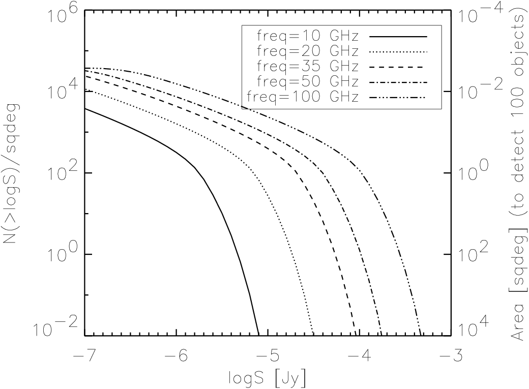
If the integral counts of sources scale as , the number of sources detected in a given area scales as . For a given flux, the number of detections is proportional to the surveyed area, i.e. to . Thus, to maximize the number of detections in a given observing time we need to go deeper if and to survey a larger area if . The number of sources detected above a given flux limit, , within a telescope FOV, , is straightforwardly derived from the source counts. The number of such pointings necessary to detect sources is and the corresponding surveyed area is . The predicted integral counts of thermal and kinetic SZ effect for several frequencies, covered by the radio interferometers mentioned above, are shown in Figs. 3 and 4, respectively. The scale on the right-hand side of these figures gives the corresponding area containing 100 protospheroids.


The time necessary to reach the wanted with in a single pointing, , is obtained from eq. (41), and the total observing time for detecting sources (excluding the slew time) is obviously . In Figs. 5 and 6 we show the on-source time for as a function of the absolute value of the thermal and kinetic SZ limiting flux for the 4 instruments in Table 1 at the frequencies specified in the inset. The curves have minima at the values of corresponding to the fastest survey capable of detecting the wanted number of sources. Clearly, it will be very time-consuming to detect 100 protospheroids with the EVLA, and unrealistic with the ATCA. On the other hand, since the 7 mm upgrade of ATCA will be operational already in 2008, it will be possible to exploit it to get the first test of the present predictions, and possibly to achieve the first detection of an SZ signal from a proto-spheroidal galaxy.
The SKA large effective collecting area allows the detection of thermal SZ signals of 100 protospheroidal galaxies at 20(10) GHz in 1(11) minutes with 7(7) pointings reaching Jy in a area. The 10% SKA requires 100 times more time than the full SKA but is still faster than EVLA or ALMA. If phased array feeds were available at the higher frequencies they would improve these surveying times by a factor of up to 50.
4.2 Redshift distributions


The redshift distributions of thermal and kinetic SZ effects are illustrated, for 3 values of , in Figs. 7 and 8. They are both relatively flat, as the fast decrease with increasing of the density of massive (i.e. SZ bright) halos is partially compensated by the brightening of SZ signals [eqs. (21) and (24)]. Such brightening is stronger for the thermal than for the kinetic SZ. A consequence of such brightening is that the range of halo masses yielding signals above a given limit shrinks with decreasing redshift, as the minimum detectable halo mass increases. The upper limit on masses of galactic halos then translates in a lower limit to the redshift distribution for bright .
4.3 Contaminant emissions
The adopted model envisages that the plasma halo has the same size as the dark matter halo, i.e. of order of hundreds kpc. In the central region (with size of order of 10 kpc), the gas cools rapidly and forms stars. Bressan, Silva, & Granato (2002) obtained a relationship between the star formation rate (SFR) and the radio luminosity at 8.4 GHz, :
| (43) |
This relationship is in good agreement with the estimate by Carilli (2001) while the equations in Condon (1992) imply a radio luminosity about a factor of 2 lower, at fixed SFR. The Granato et al. (2004) model gives the SFR as a function of galactic age, , for any value of the the halo mass and of the virialization redshift (see, e.g., Fig. 1 of Mao et al. 2007). We must, however, take into account that eq. (43) has been derived using a Salpeter (1955) Initial Mass Function (IMF). For the IMF used by Granato et al. (2004), the radio luminosity associated to a given SFR is higher by a factor of 1.6 (Bressan, personal communication). The coefficient in eq. (43) was therefore increased by this factor.
The mean rest frame luminosity at given and was then obtained using the corresponding SFR averaged over in the renormalized eq. (43). Extrapolations in frequency have been obtained using, as a template, the fit to the Arp 220 continuum spectrum obtained by Bressan et al. (2002; solid line in their Fig. 2). Using the continuum spectrum of M 82 (solid line in Fig. 1 of Bressan et al.), the other standard starburst template, we get essentially identical results.
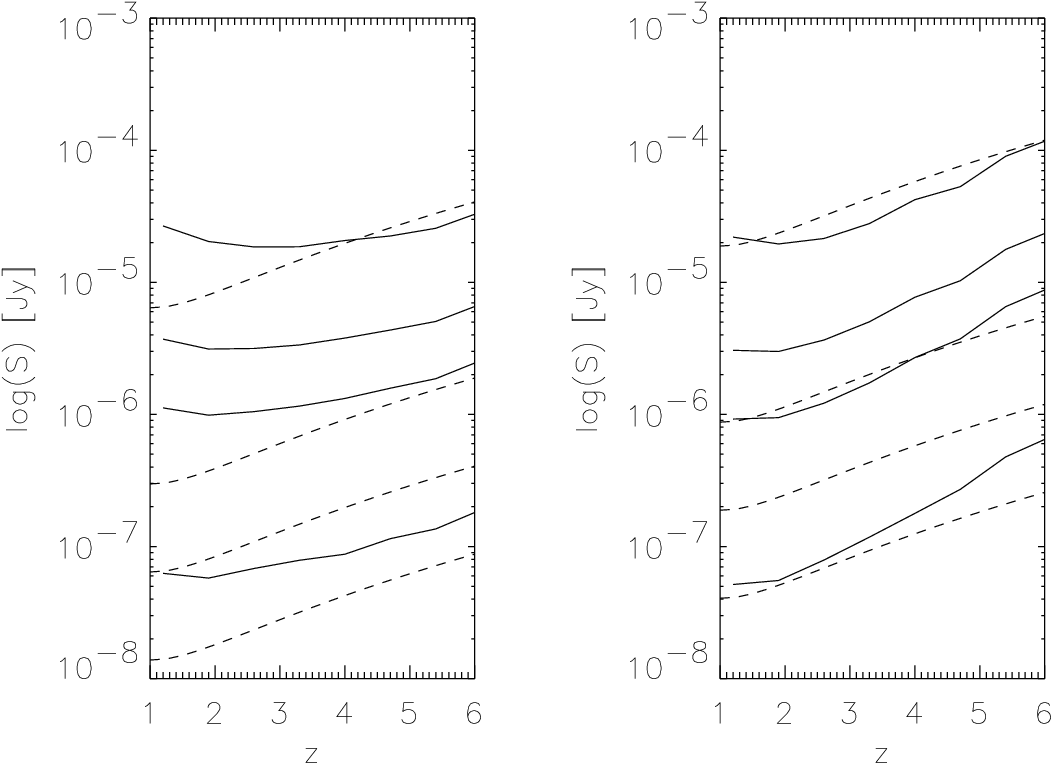
In Fig. 9 we compare the flux associated with star formation with the thermal SZ “flux” [eq. (21)], as a function of the virialization redshift, for several values of . For a given halo mass, the ratio of the thermal SZ to the contaminating signal increases with frequency (and with redshift) as far as the contamination is due to radio emission associated to star formation (we do not consider here nuclear radio emission, which occurs in per cent of galaxies). However, already at 20 GHz the thermal dust emission becomes important for the highest redshift sources. Such emission is more steeply increasing with frequency than the SZ signal, even in the Rayleigh-Jeans region of the CMB, and rapidly overwhelms it at GHz. The SZ/contamination ratio increases with increasing halo mass; therefore the SZ detection is easier for the more massive halos. Thus in the range 10–35 GHz the thermal SZ is expected to dominate over the contaminating signal at least for the most massive objects.
It must be noted that the star forming regions are concentrated in the core of the spheroids, on angular scales of the order or less than , for the redshifts considered here. Long ( at for full sensitivity) baselines observation with high sensitivity may be able to resolve the star forming region positive signal and subtract it from the image. To achieve this purpose a good sampling of the shortest spacings on the uv plane is necessary together with a good sampling of the largest ones: with the latter it might be possible to reconstruct the contaminated profile, subtract it from the former and produce an uncontaminated SZ profile. Again, the SKA at high frequencies seems to be the optimal instrument.
4.4 Confusion effects
Further constraints to the detection of SZ effects are set by confusion fluctuations. Fomalont et al. (2002) have determined the 8.4 GHz source counts down to Jy. For mJy they are well described by:
| (44) |
with in Jy. The spectral index distribution peaks at ().
For all but one (SKA 10 GHz) of the considered surveys the “optimal” depth for detecting 100 sources corresponds to 8.4 GHz flux densities within the range covered by Fomalont et al. (2002), so that the confusion fluctuations are dominated by sources obeying eq. (44). We then have:
| (45) |
where , in Jy, is the detection limit and is the solid angle subtended by the SZ signal. Equation (45) can be rewritten as
| (46) |
yielding a detection limit of Jy at 10 GHz and of Jy at 20 GHz. For the “optimal” survey depths at higher frequencies , implying that they are not affected by confusion noise due to radio sources.
On the other hand, as noted above, at high frequencies the redshifted dust emission from distant star-forming galaxies becomes increasingly important (De Zotti et al. 2005). To estimate their contribution to the confusion noise, we have used once again the model by Granato et al. (2004), with the dust emission spectra revised to yield counts consistent with the results by Coppin et al. (2006), and complemented by the phenomenological estimates by Silva et al. (2004, 2005) of the counts of sources other than high- proto-spheroids (see Negrello et al. (2007) for further details). We find, for a typical solid angle , flux limits due to these sources of 3, 55, and Jy at 20, 35, and 50 GHz, respectively. Thus at 20 GHz we have significant contributions to the confusion noise both from the radio and from the dust emission; the overall detection limit is Jy. At 10 GHz the contribution of dusty galaxies to the confusion noise is negligible, while at 100 GHz the confusion limit is as high as 2 mJy, implying that the detection of the galactic-scale SZ effect is hopeless at mm wavelengths.
Although high- luminous star-forming galaxies may be highly clustered (Blain et al. 2005; Farrah et al. 2006; Magliocchetti et al. 2007), the clustering contribution to fluctuations is negligible on the small scales of interest here (De Zotti et al. 1996), and can safely be neglected.
5 Conclusions
In the standard scenario for galaxy formation, the proto-galactic gas is shock heated to the virial temperature. The observational evidences that massive star formation activity must await the collapse of large halos, a phenomenon referred to as downsizing, suggest that proto-galaxies with a high thermal energy content existed at high redshifts. Such objects are potentially observable through the thermal and kinetic Sunyaev-Zel’dovich effects and their free-free emission. The detection of this phase of galaxy evolution would shed light on the physical processes that govern the collapse of primordial density perturbations on galactic scales and on the history of the baryon content of galaxies.
As for the latter issue, the standard scenario, adopted here, envisages that the baryon to dark matter mass ratio at virialization has the cosmic value, i.e. is about an order of magnitude higher than in present day galaxies. Measurements of the SZ effect will provide a direct test of this as yet unproven assumption, and will constrain the epoch when most of the initial baryons are swept out of the galaxies.
As mentioned in § 1, almost all semi-analytic models for galaxy formation adopt halo mass functions directly derived or broadly consistent with the results of N-body simulations, and it is commonly assumed that the gas is shock heated to the virial temperature of the halo. They therefore entail predictions on counts of SZ effects similar to those presented here. On the other hand, the thermal history of the gas is governed by a complex interplay of many astrophysical processes, including gas cooling, star formation, feedback from supernovae and active nuclei, shocks. As mentioned in § 1, recent investigations have highlighted that a substantial fraction of the gas in galaxies may not be heated to the virial temperature. Also, it is plausible that the AGN feedback transiently heats the gas to temperatures substantially above the virial value, thus yielding SZ signals exceeding those considered here. The gas thermal history may therefore be substantially different from that envisaged by semi-analytic models, and the SZ observations may provide unique information on it.
We have presented a quantitative investigation of the counts of SZ and free-free signals in the framework of the Granato et al. (2004) model, that successfully accounts for the wealth of data on the cosmological evolution of spheroidal galaxies and of AGNs (Granato et al. 2004; Cirasuolo et al. 2005; Silva et al. 2005; Lapi et al. 2006).
We find that the detection of substantial numbers of galaxy-scale thermal SZ signals is achievable by blind surveys with next generation radio interferometers. Since the protogalaxy thermal energy content increases, for given halo mass, with the virialization redshift, the SZ “fluxes” increase rather strongly with , especially for the thermal SZ effect, partially compensating for the rapid decrease of the density of massive halos with increasing redshift. The redshift distributions of thermal SZ sources are thus expected to have substantial tails up to high .
There are however important observational constraints that need to be taken into account. The contamination by radio and dust emissions associated to the star formation activity depends on mass and redshift of the objects, but is expected to be stronger than the SZ signal at very low and very high frequencies. We conclude that the optimal frequency range for detecting the SZ signal is from 10 to 35 GHz, where such signal dominates over the contamination at least for the most massive objects. It must be noted however that contaminating emissions have typical scales of the order of those of the stellar distributions, i.e. at the redshifts of interest here (see Fomalont et al. 2006), while the SZ effects show up on the scale of the dark matter halo, which is typically ten times larger. Therefore arcsec resolution images, such as those that will be provided by the SKA, will allow to reconstruct the uncontaminated SZ signal.
The coexistence of the hot plasma halo, responsible for the SZ signal, with dust emission implies that the scenario presented in this paper may be tested by means of pointed observations of high- luminous star-forming galaxies detected by (sub)-mm surveys.
Confusion noise is a very serious limiting factor at mm wavelengths. Contributions to confusion come on one side from radio sources and on the other side from dusty galaxies. At 10 GHz only radio sources matter; a modest extrapolation of the 8.4 GHz Jy counts by Fomalont et al. (2002) gives a detection limit Jy, for a SZ signal subtending a typical solid angle of . Fluctuations due to dust emission from high- luminous star-forming galaxies may start becoming important already at 20 GHz; at this frequency, quadratically summing them with those due to radio sources we find again Jy, for the same solid angle. On the other hand, the high resolution of the SKA and of the EVLA will allow us to effectively detect and subtract out confusing sources, thus substantially decreasing the confusion effects. Beating confusion will be particularly important for searches of the weaker kinetic SZ signal.
ACKNOWLEDGMENTS
We are indebted to G. L. Granato for having provided the software
to compute the cooling function and the halo mass function, to A.
Diaferio for explanations on the halo velocity function and its
cosmological evolution, and to A. Bressan for clarifications on
the dependence of the radio-luminosity/SFR relation on the IMF.
We thank M. Rupen for updated information about the EVLA capabilities.
We also warmly thank the anonymous referee for an unusually
accurate reading of the manuscript and for many constructive
comments.
Work supported in part by the Ministero dell’Università e della
Ricerca and by ASI (contract Planck LFI Activity of Phase E2).
References
- Benson et al. (2003) Benson A. J., Bower R. G., Frenk C. S., Lacey C. G., Baugh C. M., Cole S., 2003, ApJ, 599, 38
- Binney (2004) Binney J., 2004, MNRAS, 347, 1093
- Birkinshaw & Lancaster (2005) Birkinshaw M., Lancaster K., 2005, Proc. of the International School of Physics ”Enrico Fermi”, ”Background Microwave Radiation and Intracluster Cosmology”, p. 127
- Birnboim & Dekel (2003) Birnboim Y., Dekel A., 2003, MNRAS, 345, 349
- Blain et al. (2005) Blain A. W., Chapman S. C., Smail I., Ivison R., 2005, proc. ESO workshop on ”Multiwavelength Mapping of Galaxy Formation and Evolution”, p. 94
- Bower et al. (2006) Bower R. G., Benson A. J., Malbon R., Helly J. C., Frenk C. S., Baugh C. M., Cole S., Lacey C. G., 2006, MNRAS, 370, 645
- Bressan, Silva, & Granato (2002) Bressan A., Silva L., Granato G. L., 2002, A&A, 392, 377
- Bryan & Norman (1998) Bryan G. L., Norman M. L., 1998, ApJ, 495, 80
- Bullock et al. (2001) Bullock J. S., Kolatt T. S., Sigad Y., Somerville R. S., Kravtsov A. V., Klypin A. A., Primack J. R., Dekel A., 2001, MNRAS, 321, 559
- Carilli (2001) Carilli C. L., 2001, in “Starburst Galaxies: Near and Far”, L. Tacconi & D. Lutz, eds., Heidelberg: Springer-Verlag, p. 309
- Carlstrom, Holder, & Reese (2002) Carlstrom J. E., Holder G. P., Reese E. D., 2002, ARA&A, 40, 643
- Cirasuolo et al. (2005) Cirasuolo M., Shankar F., Granato G. L., De Zotti G., Danese L., 2005, ApJ, 629, 816
- Cole (1991) Cole S., 1991, ApJ, 367, 45
- Cole et al. (1994) Cole S., Aragon-Salamanca A., Frenk C.S., Navarro J.F., Zepf S.E., 1994, MNRAS, 271, 781
- Condon (1992) Condon J. J., 1992, ARA&A, 30, 575
- Croton et al. (2006) Croton D. J., et al., 2006, MNRAS, 365, 11
- Dekel & Birnboim (2006) Dekel A., Birnboim Y., 2006, MNRAS, 368, 2
- Dekel & Silk (1986) Dekel A., Silk J., 1986, ApJ, 303, 39
- de Zotti et al. (1996) de Zotti G., Franceschini A., Toffolatti L., Mazzei P., Danese L., 1996, ApL&C, 35, 289
- de Zotti et al. (2004) de Zotti G., Burigana C., Cavaliere A., Danese L., Granato G. L., Lapi A., Platania P., Silva L., 2004, AIPC, 703, 375
- de Zotti et al. (2005) de Zotti G., Ricci R., Mesa D., Silva L., Mazzotta P., Toffolatti L., González-Nuevo J., 2005, A&A, 431, 893
- Farrah et al. (2006a) Farrah D., et al., 2006, ApJ, 641, L17 (erratum: 2006, ApJ, 643, L139)
- Fomalont et al. (2002) Fomalont E. B., Kellermann K. I., Partridge R. B., Windhorst R. A., Richards E. A., 2002, AJ, 123, 2402
- Fomalont et al. (2006) Fomalont E. B., Kellermann K. I., Cowie L. L., Capak P., Barger A. J., Partridge R. B., Windhorst R. A., Richards E. A., 2006, ApJS, 167, 103
- Granato et al. (2001) Granato G. L., Silva L., Monaco P., Panuzzo P., Salucci P., De Zotti G., Danese L., 2001, MNRAS, 324, 757
- Granato et al. (2004) Granato G. L., De Zotti G., Silva L., Bressan A., Danese L., 2004, ApJ, 600, 580
- Haehnelt & Rees (1993) Haehnelt M. G., Rees M. J., 1993, MNRAS, 263, 168
- Hogg (1999) Hogg D. W., 1999, astro, arXiv:astro-ph/9905116
- Itoh et al. (2000) Itoh N., Sakamoto T., Kusano S., Nozawa S., Kohyama Y., 2000, ApJS, 128, 125
- (30) Katz N., Kereš D., Davé R., Weinberg D.H., 2003, in Rosenberg J.L., Putman M.E., eds, The IGM/Galaxy Connection: the Distribution of Baryons at z = 0. Kluwer, Dordrecht, p. 185
- Kauffmann, White, & Guiderdoni (1993) Kauffmann G., White S. D. M., Guiderdoni B., 1993, MNRAS, 264, 201
- Kereš et al. (2005) Kereš D., Katz N., Weinberg D. H., Davé R., 2005, MNRAS, 363, 2
- Koopmans et al. (2006) Koopmans L. V. E., Treu T., Bolton A. S., Burles S., Moustakas L. A., 2006, ApJ, 649, 599
- Lacey & Silk (1991) Lacey C., Silk J., 1991, ApJ, 381, 14
- Lapi, Cavaliere, & De Zotti (2003) Lapi A., Cavaliere A., De Zotti G., 2003, ApJ, 597, L93
- Lapi et al. (2006) Lapi A., Shankar F., Mao J., Granato G. L., Silva L., De Zotti G., Danese L., 2006, ApJ, 650, 42
- Larson (1974) Larson R.B., 1974, MNRAS, 169, 229
- Magliocchetti et al. (2007) Magliocchetti M., Silva L., Lapi A., De Zotti G., Granato G.L., Fadda D., Danese L., 2007, MNRAS, 375, 1121
- Majumdar, Nath, & Chiba (2001) Majumdar S., Nath B. B., Chiba M., 2001, MNRAS, 324, 537 (erratum: 2001, MNRAS, 326, 1216)
- Mao et al. (2007) Mao J., Lapi A., Granato G. L., de Zotti G., Danese L., 2007, ApJ, submitted, astro-ph/0611799
- Navarro, Frenk & White (1997) Navarro J. F., Frenk C. S., White S. D. M., 1997, ApJ, 490, 493
- Negrello et al. (2007) Negrello M., Perrotta F., González J. G.-N., Silva L., de Zotti G., Granato G. L., Baccigalupi C., Danese L., 2007, MNRAS, 323
- Oh (1999) Oh, S. P., 1999, ApJ, 527, 16-30.
- Oh, Cooray, & Kamionkowski (2003) Oh S. P., Cooray A., Kamionkowski M., 2003, MNRAS, 342, L20
- Platania et al. (2002) Platania P., Burigana C., De Zotti G., Lazzaro E., Bersanelli M., 2002, MNRAS, 337, 242
- Rees & Ostriker (1977) Rees M. J., Ostriker J. P., 1977, MNRAS, 179, 541
- Renzini (2006) Renzini A., 2006, ARA&A, 44, 141
- Ribicky & Lightman (1979) Rybicki G. B., Lightman A. P., 1979, ”Radiative processes in astrophysics”, New York Wiley
- Rosa-González et al. (2004) Rosa-González D., Terlevich R., Terlevich E., Friaça A., Gaztañaga E., 2004, MNRAS, 348, 669
- Salpeter (1955) Salpeter E. E., 1955, ApJ, 121, 161
- Sasaki (1994) Sasaki S., 1994, PASJ, 46, 427
- Sheth & Tormen (1999) Sheth R. K., Tormen G., 1999, MNRAS, 308, 119
- Sheth & Diaferio (2001) Sheth R. K., Diaferio A., 2001, MNRAS, 322, 901
- Silva et al. (2004) Silva L., De Zotti G., Granato G. L., Maiolino R., Danese L., 2004, astro, arXiv:astro-ph/0403166
- Silva et al. (2005) Silva L., De Zotti G., Granato G. L., Maiolino R., Danese L., 2005, MNRAS, 357, 1295
- Silva et al. (1998) Silva L., Granato G. L., Bressan A., Danese L., 1998, ApJ, 509, 103
- Somerville & Primack (1999) Somerville R.S., Primack J.R., 1999, MNRAS, 310, 1087
- Spergel et al. (2006) Spergel D. N., et al., 2006, astro, arXiv:astro-ph/0603449
- Sunyaev & Zel’dovich (1972) Sunyaev R. A., Zel’dovich Y. B., 1972, CoASP, 4, 173
- Thomas, Maraston, & Bender (2002) Thomas D., Maraston C., Bender R., 2002, RvMA, 15, 219
- Wechsler et al. (2002) Wechsler R.H., Bullock J.S., Primack J.R., Kravtsov A.V., Dekel A., 2002, ApJ, 568, 52
- White & Frenk (1991) White S. D. M., Frenk C. S., 1991, ApJ, 379, 52
- White & Rees (1978) White S. D. M., Rees M. J., 1978, MNRAS, 183, 341
- Zhao et al. (2003a) Zhao D.H., Jing Y.P., Mo H.J., Börner G., 2003b, ApJ, 597, L9
- Zhao et al. (2003b) Zhao D.H., Mo H.J., Jing Y.P., Börner G., 2003a, MNRAS, 339, 12