CERN-PH-TH/2007-206
SACLAY-T07/142
Gravitational wave generation from bubble collisions in first-order phase transitions: an analytic approach
Chiara Caprinia,b, Ruth Durrera and Géraldine Servant b,c
a Département de Physique Théorique, Université de Genève,
24 Quai E. Ansermet, CH-1211 Genève, Switzerland
bService de Physique Théorique, CEA Saclay, F91191 Gif–sur–Yvette, France
cCERN Physics Department, Theory Division, CH-1211 Geneva 23, Switzerland
chiara.caprini@cea.fr, Ruth.Durrer@physics.unige.ch, geraldine.servant@cern.ch
Abstract
Gravitational wave production from bubble collisions was calculated in the early nineties using numerical simulations. In this paper, we present an alternative analytic estimate, relying on a different treatment of stochasticity. In our approach, we provide a model for the bubble velocity power spectrum, suitable for both detonations and deflagrations. From this, we derive the anisotropic stress and analytically solve the gravitational wave equation. We provide analytical formulae for the peak frequency and the shape of the spectrum which we compare with numerical estimates. In contrast to the previous analysis, we do not work in the envelope approximation. This paper focuses on a particular source of gravitational waves from phase transitions. In a companion article, we will add together the different sources of gravitational wave signals from phase transitions: bubble collisions, turbulence and magnetic fields and discuss the prospects for probing the electroweak phase transition at LISA.
1 Introduction
In the next decades, a new science will emerge from direct detection of gravitational radiation, that will open a qualitatively new way of probing the distant universe. Ground-based (LIGO [1] and VIRGO [2]) and space-based (LISA [3]) interferometers will reach the required sensitivity to detect many kinds of distant sources over a range of more than a million in frequency. Because gravitational waves (GW) penetrate all regions of time and space, with almost no attenuation, GW detectors can explore scales, epochs and new physical effects not accessible in any other way.
Although the first GW detections will come from astrophysical processes, such as merging of black holes, another mission of GW astronomy will be to search for a stochastic background of GWs of primordial origin. An important mechanism for generating such a stochastic GW background is a relativistic first-order phase transition [4, 5]. In a first-order phase transition, bubbles are nucleated, rapidly expand and collide. The free energy contained in the original vacuum is released and converted into thermal energy and kinetic energy of the bubble walls and the surrounding fluid. Most of the gravitational radiation comes from the final phase of the transition, from many-bubble collisions and the subsequent MHD turbulent cascades. The associated GW spectrum encodes information on the temperature of the universe at which the waves were emitted as well as on the strength of the transition. The characteristic frequency of the waves corresponds to the physics that produces them. For cosmological processes, this is close to the Hubble frequency, . Once redshifted to today, this corresponds to
| (1) |
Remarkably, for transitions occuring near the electroweak epoch, is in the frequency range covered by LISA ( Hz). It is therefore very exciting that LISA could help probing the nature of the electroweak phase transition, and therefore provide information that is complementary to the Large Hadron Collider and the future International Linear Collider.
Many types of new physics predict first-order phase transitions. Electroweak symmetry breaking in extensions of the Standard Model may be associated with a first-order phase transition (see for example Ref. [6]). Besides, the last decade has seen the emergence of the “landscape picture”, following developments in String Theory. Strongly warped regions (throats) in higher-dimensional space-time are generic features in the string-theory landscape [7] and the phenomenological consequences are only starting to be explored (for instance through the prototype of Randall and Sundrum [8]). One interesting aspect is the cosmological evolution in these backgrounds. Thanks to holography and the AdS-CFT correspondence, a change in the 5-dimensional metric as the temperature decreases can be understood as a confining phase transition in the dual 4-dimensional gauge theory, and in models like [8], we typically expect first-order phase transitions at the TeV scale [9, 10, 11, 12, 13]. Finally, phenomena such as preheating at the end of inflation could share some common features, as far as gravity wave emission is concerned, with the physics of first-order phase transitions [14, 15, 16].
The GW spectrum resulting from bubble collisions in first order phase transitions was computed in the early nineties [18, 17, 19, 20]. It was realized ten years after the original calculation of [18, 17, 19, 20] that turbulence in the plasma could be a significant source of GW in addition to bubble collisions [21, 22]. Subsequently, the authors of [23] studied the GW signal due to a first order electroweak phase transition in the Minimal Supersymmetric Standard Model (MSSM) and its NMSSM extension. More recently, model-independent analysis for the detectability of GW with LISA [24, 25], LIGO and BBO [25] were presented, relying on the formulae derived in [18, 17, 19, 20, 21, 22]. The spectrum derived in Ref. [18, 17, 19, 20] was estimated using numerical simulations, and no alternative calculation was performed afterwards. As argued above, we believe this is of high interest and it is time to revisit this question. In this paper, we present an analytical calculation of the stochastic GW background resulting from bubble collisions only11 1 Turbulent fluid motions triggered by bubble collisions together with magnetic fields are actually additional relevant sources for gravity waves from phase transitions. These effects have been reexamined recently [26, 27, 28] and since the subject is not closed, we will present revisited results from these contributions elsewhere [29].. Since bubble collisions take place in a thermal bath, and since we want to extend our treatment to deflagrations, we use the energy-momentum tensor of the relativistic fluid in the vicinity of the bubble wall as the GW source, rather than the energy-momentum of the scalar field. The result we find is comparable to that obtained by numerical simulations although the peak frequency is parametrically larger.
A deterministic spherically symmetric expanding bubble does not produce gravitational radiation by itself. The reason is, that the transverse and traceless part of the energy momentum tensor for a radial deterministic distribution of the velocity field is identically zero (as we demonstrate in Appendix A). To produce a non-zero background of GW, one has to account for the fact that, towards the end of the phase transition, the collision of bubbles breaks spherical symmetry and leads to a non-zero tensor anisotropic stress. In the numerical simulations of Refs. [17, 19, 20], this is accounted for by evaluating the transverse traceless component of an “incomplete” energy momentum tensor coming from the portion of bubble wall that remains uncollided at a given time. This energy momentum tensor is not spherically symmetric and has a non-zero tensor anisotropic stress component. The total tensor anisotropic stress is obtained by summing all the contributions from single uncollided bubble walls. Each simulation provides a given configuration of uncollided bubble walls; bubble nucleation and collision being random processes, the GW power spectrum is obtained by averaging the results of several simulations. This procedure is valid under the thin-wall “envelope” approximation, i.e. when the transition is strong and the bubble front evolves as a detonation.
In the analytical evaluation which we present here, the situation is quite different. The GW production comes not only from the bubble wall, but from the entire fluid velocity profile in the vicinity of the phase discontinuity. If the non-zero fluid velocity shell contracts to a surface with vanishing thickness, no gravitational waves are produced. Therefore, we are not working in the thin wall approximation, and this is why we are able to apply our results also to the case of deflagrations.
The paper is organized as follows. In Section 2 we review the general procedure for calculating the relic energy density stored in a stochastic background of gravitational waves. Section 3 describes our model of the GW source, the calculation of the bubble velocity power spectrum and the anisotropic stress power spectrum. In Section 4 we define the time dependence of the phase transition parameters. In Section 5 the calculation of the GW spectrum, applicable both for detonations and deflagrations is presented. In Section 6, we make some comments on our analytical approach. In the last section we collect our final results and compare them with the existing formulae used in in the literature. Some technical aspects related to the calculation of the velocity power spectrum are collected in Appendix B. Appendix C is a discussion on the behaviour of the small and large scale tails of the GW power spectrum. While the existing literature provides approximate expressions for the peak amplitude and peak frequency of the signal, there is no justification for the shape of the spectrum. Our analytical approach provides a rationale for it based on simple dimensional arguments.
2 Gravitational wave power spectrum: general remarks
Our goal is to estimate the gravitational wave energy density generated by bubbles during a first-order phase transition. This kind of cosmological source leads to a stochastic background of GW, which is isotropic, stationary, unpolarized and therefore characterized entirely by its frequency spectrum [30]. We consider a Friedmann universe with flat spatial sections. The tensor metric perturbations are defined by
| (2) |
The gravitational wave energy density is then given by
| (3) |
The over-dot denotes derivative with respect to conformal time and denotes both time averaging over several periods of oscillation and ensemble average for a stochastic background. The variables and later also denote comoving distances, and later , denote comoving time. The density parameter is always scaled to today, , where the index 0 indicates the present time. For relativistic species we have therefore ; we normalize and sometimes denote the present value of a density parameter simply by ; likewise, . denotes the conformal Hubble parameter. The radiation energy density today is taken to be [31].
We define the statistically homogeneous and isotropic gravitational wave energy density spectrum by
| (4) |
where is the comoving wave vector. The gravitational wave energy density, normalized to the critical energy density is:
| (5) |
where the factor comes from the Fourier transform convention. We want to estimate the present day gravitational wave energy spectrum, in other words the gravitational wave energy density per logarithmic frequency interval,
| (6) |
In an expanding radiation-dominated universe, is the solution of the wave equation
| (7) |
is the tensor part of the anisotropic stress, the transverse-traceless component of the energy momentum tensor that generates tensor perturbations of the metric:
| (8) |
where is the transverse projector and are the spatial components of the energy momentum tensor. As will be discussed in the next section, the anisotropic stress is a stochastic variable for the generation process under consideration. It accounts for the intrinsic randomness of bubble nucleation and collision.
Our source of gravitational radiation is active for an interval of time corresponding to the duration of the phase transition, which is much shorter than one Hubble time [32, 33]. We can therefore neglect the expansion of the universe while the source is still active, and rewrite Eq. (7) as
| (9) |
where , ′ denotes derivative with respect to and is the scale factor at the time of the phase transition. The dependence of on directions of the wave-vector enters only in the polarization of the wave and is irrelevant for our discussion. As will become clear at the end of this section, in Eq. (16), this is due to statistical homogeneity and isotropy of the source. We assume that the source turns on at time and turns off at time . The solution of (9) is
| (10) |
where ( denotes conformal time) and is the Green function satisfying and . Once the source is no longer active, we have to match the above solution with the solution of the free wave equation during radiation domination
| (11) | |||
| (12) |
The matching procedure gives the coefficients
| (13) |
In order to simplify the equations, we neglect the first term in which gives a subdominant contribution to the GW spectrum in the range of frequencies we are interested in. In fact, this term contributes in a sizable way only for modes larger than the horizon,
| (14) |
where denotes the conformal Hubble factor at the time of the phase transition, and is assumed to be constant from to since the phase transition lasts for a time much shorter than one Hubble time. We will see that the GW spectrum grows very steeply at large scales (as ) and peaks at a scale corresponding to the maximal size of the bubbles, which is typically much smaller than the horizon. Therefore, we are mainly interested in the sub-horizon part of the spectrum and in order to evaluate it we can safely neglect the term . Using definition (4) and solution (12) we finally find ()
| (15) | |||||
In the double integral above, we have combined the products of two Green’s functions into the simpler term . Moreover, we have introduced the unequal time correlator of the tensor anisotropic stress in Fourier space,
| (16) |
The delta function is due to the statistical homogeneity of the source, and because of statistical isotropy the power spectrum of the anisotropic stress only depends on the wave number. Note that for the matching we have used the free wave propagation equation (11), which is valid in an expanding, radiation dominated universe with . Hence, solution (15) for implicitly assumes that the number of relativistic degrees of freedom is constant. We come back to this issue in section 5.
To summarize, in order to determine the spectrum of the gravitational radiation Eq. (6), we have to calculate the power spectrum of the anisotropic stress evaluated at different times. This requires computing the correlator of the energy momentum tensor. The next section is devoted to a calculation of (Eq. 16). For this we need a model of the energy momentum tensor that sources the gravitational waves.
3 Model of the GW source
We now develop a model for the stochastic source of gravitational radiation. We are dealing with a cosmological first order phase transition taking place in a thermal bath [34, 20]. The cosmic fluid of the initial metastable phase supercools until the nucleation of bubbles of the final phase can start. The initial high-temperature phase or false vacuum is typically but not necessarily the symmetric phase. However, in the remaining of the paper, we will use the term “symmetric” for the initial phase and “broken” for the final phase. The phase transition ends when the entire universe has been converted to the broken phase by bubble percolation. We are only interested in the last stages of bubble growth. Towards the end of the phase transition, the bubbles can be considered simply as spherical combustion fronts moving at constant velocity [35]. Any memory of the initial shape of the bubbles, driven by the scalar field dynamics, is lost and the problem can be reduced to a purely hydrodynamical description. The bubbles are modeled as spherically symmetric configurations of fluid velocity. The velocity field is a stochastic variable, following the intrinsic stochasticity of the nucleation process.
3.1 Anisotropic stress power spectrum: general remarks
Since we are interested only in the anisotropic stress, we start with the spatial, off-diagonal part of the energy momentum tensor of the cosmic fluid, quantifying the spatial components of the kinetic stress-energy tensor of a bubble configuration [20]:
| (17) |
is the velocity of the fluid in the frame of the bubble center, and . We want to calculate the anisotropic stress power spectrum given in Eq. (16). In order to simplify the calculation, we neglect the spatial dependence of the fluid enthalpy density and of the gamma factor . This assumption is necessary in order to be able to proceed analytically. It supposes that the only stochastic variables in the problem are the fluid velocity components , and that the spatially dependent factor can be approximated by . The consequences of this assumption cannot be quantified exactly. However, we know that varies smoothly from to (see Eq. 29) where and are defined in Eq. 3.2. A conservative choice is to always set to its smallest value, and this is what we will do in Eqs. (64) and (65). Under these assumptions, we can write the Fourier transform,
| (18) |
With this expression, the power spectrum of the energy momentum tensor involves the four-point function of the velocity distribution:
| (19) | |||||
There is in principle no reason why our stochastic velocity field should have a Gaussian distribution. However, we have to make some assumptions in order to calculate analytically the four-point function in the above expression. As one often does, we assume that Wick’s theorem, which is strictly valid only for Gaussian random variables, gives a good enough approximation to the four-point function. It certainly gives a better estimate than, for example, the simple product of expectation values. Applying it we find
| (20) | |||||
where
| (21) |
The correlation between point and point is a function of only because of statistical homogeneity.
In our approach, the ensemble average in Eq. (3) is now traced back into a correlator for the bubble velocities. This is where the stochasticity of the process is encoded. Since the velocity field is statistically homogeneous and isotropic, its power spectrum has the general form (see the next subsection 3.2.1)
| (22) |
The power spectrum of the tensor part of the anisotropic stress is calculated using the definition (16) by applying the transverse traceless projector as in Eq. (8):
| (23) |
A somewhat lengthy calculation yields
| (24) | |||||
where and and we have suppressed the time variables and in and .
3.2 Velocity profile of bubbles
Since we are only interested in the last stage of the phase transition, we consider the hydrodynamics of bubble growth at late times, when a steady state solution is reached. The bubble wall, in other words the combustion front where the phase transition is happening, is moving at constant velocity. In the hydrodynamical description of the combustion, the front is treated as a surface of discontinuity. Energy and momentum must be conserved across the front and all the entropy production is confined to it [34, 35]. Elsewhere, the fluid is in a state of thermal equilibrium. The energy momentum tensor of the burnt (broken) and unburnt (symmetric) phases is simply that of two perfect fluids (see Eq. 17). There are two kinds of solutions to this hydrodynamical problem, detonations and deflagrations. These are classified following the characteristics of the fluid flow in the rest frame of the combustion front [36, 37].
In detonations, the incoming velocity of the symmetric phase fluid into the front is supersonic in the rest frame of the front. The outgoing velocity of the broken phase fluid out of the front can be supersonic for weak detonations, or equal to the speed of sound for Jouguet detonations . The case of strong detonations is forbidden [36]. Although weak detonations are possible [38], in the following we concentrate for simplicity on the case of Jouguet detonations. This is the case analyzed in [20], for which the dynamics of the bubble growth is completely determined in terms of the phase transition strength. Since both fluid phases are relativistic, they have the sound speed . In the rest frame of the bubble center, the velocity of the bubble front is supersonic, corresponding to : the symmetric phase fluid is therefore at rest, and the front is followed by a rarefaction wave in the broken phase fluid. The rarefaction wave brings the fluid motion to rest towards the center of the bubble. Near the detonation front, the broken phase fluid velocity in the rest frame of the center of the bubble is simply given by the Lorentz transformation
| (25) |
The velocity profile of the broken phase fluid for a Jouguet detonation has been studied in detail in Refs. [36, 34, 20] and is shown schematically in the first panel of Fig. 1. As customary, we show the velocity profile as a function of the parameter . Here is the time of bubble nucleation and denotes the distance form the bubble center22 2 Throughout this section, for simplicity we use a generic time variable ; we switch back to comoving time in paragraph 3.2.2.. We remind that this situation corresponds to the steady state solution at late times, long after the nucleation time. The velocity of the broken phase fluid goes to zero in the interior of the bubble at a distance from the center corresponding to [36].

For deflagrations, on the other hand, the incoming velocity of the symmetric phase fluid into the front is subsonic . The outgoing velocity of the broken phase fluid out of the front can be subsonic for weak deflagrations, or equal to the speed of sound for Jouguet deflagrations . Strong deflagrations are again impossible [36]. In the rest frame of the bubble center, the velocity of the bubble front corresponds in this case to . The front moves at subsonic velocity and is therefore preceded in the symmetric phase by a shock wave. Inside the combustion bubble (broken phase) and outside the shock wave (symmetric phase) the fluid is at rest; in between, the fluid moves outwards. In the case of planar deflagrations, it does so at constant velocity given by (Eq. 25) [36, 35]. The qualitative features of the velocity profile for a planar deflagration are shown in the second panel of Fig. 1 33 3 In Appendix A of Ref. [20] it is shown that, in the case of spherical deflagrations, the velocity profile actually decreases between and . We do not account for this behaviour here, since in any case we are forced to introduce an approximate form for the velocity profile..
For our analytic calculation, we want to simplify the real velocity profile both for detonations and deflagrations. We assume a velocity profile which grows linearly within a shell near the bubble wall, as shown in the last panel of Fig. 1. We have normalized the velocity profile at the outer boundary (bubble wall or shock front) to the correct value for detonations and deflagrations. This is because the biggest contribution to the GW energy density comes from the highest velocity region. Therefore, our approximated profile does reproduce the most relevant feature as far as GW generation is concerned. The boundaries of the shell, defined as and in Fig. 1 are left as free parameters, in order to allow for an approximated description of both detonations and deflagrations.
The simplified profile is
Here is the position of the bubble center. The radii of the shell’s inner and outer boundaries are respectively and , where is much later than the nucleation time . In the case of Jouguet detonations, the inner boundary is in the broken phase and corresponds to . For deflagrations, it corresponds to the bubble wall, . The radius of the outer boundary is and for detonations it is associated to the bubble wall velocity , while for deflagrations to the shock front . To summarize:
| Detonations | Deflagrations | |
The numerical values of , and will be crucial in determining the amplitude of the GW signal and will be discussed in Sections 5.2 and 5.3. A schematic drawing of the bubble (or shock front) is given in Fig. 2.

3.2.1 Velocity power spectrum
Given the velocity profile, we can proceed to calculate the velocity power spectrum. We start by evaluating the two-point correlation function at equal time for fixed positions and defined in Eq. (21). The position of the bubble center defined in Eq. (3.2) is the stochastic variable. Therefore, in the region of non-zero velocity we have:
| (29) |
where we remind that is the maximal value of the fluid velocity in the rest frame of the bubble center. For the velocity correlation function not to be zero, and must be separated by a distance and they have to be in the same bubble (or shock wave, in the case of deflagrations). Moreover, they have to be in the shell where the fluid velocity (3.2) is not zero. These conditions are satisfied provided that the center of the bubble they belong to is in a volume given by the intersection of two shells centered in and , which have inner radius and outer radius (see Fig. 3). Therefore, the correlation function is given by the mean over all the possible center positions within this intersection volume, multiplied by the probability that there actually is a bubble center in this region:
| (30) |
As customary in cosmology, here we use the ergodic assumption: ensemble averages are equivalent to space averages. The probability of having a bubble center in the intersection region is simply given by
| (31) |
where is the fraction of volume occupied by bubbles at time , and is the volume of the region where can be, in order for or to be in the same bubble: the total volume of the two overlapping spheres in Fig. 3. Setting we find
| (32) |
The tensorial structure of the two-point correlation function of a statistically homogeneous and isotropic field is known: the correlation function can only depend on the distance between and . We choose an orthonormal basis with . The off-diagonal components of the integral in Eq. (30) are zero by symmetry, and therefore we find
| (33) | |||||
| (34) | |||||
| (35) |
(since ). The functions and have to be calculated by performing the necessary integration in the four volume regions shown in Fig. 3. The details of the calculations are given in Appendix B.


The velocity power spectrum is then obtained by Fourier transforming the two point correlation function (34) with respect to the variable . Remembering the definitions (21,22) one finds the general expressions ( denotes the Fourier transform)
| (36) | |||||
| (37) | |||||
| (38) |
where we remind that is defined below Eq. (31).
We define the new dimensionless variable and the fraction
| (39) |
Note that is the relative thickness of the shell, and will contribute to the amplitude of the GW signal. In our approach, the GW signal will vanish in the limit of vanishing thickness. We perform the Fourier transform and obtain the following expression for the velocity power spectrum:
| (40) |
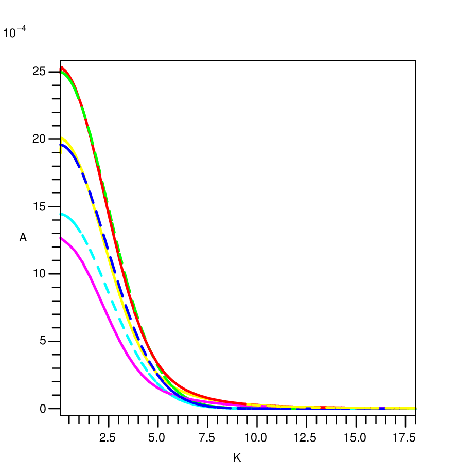
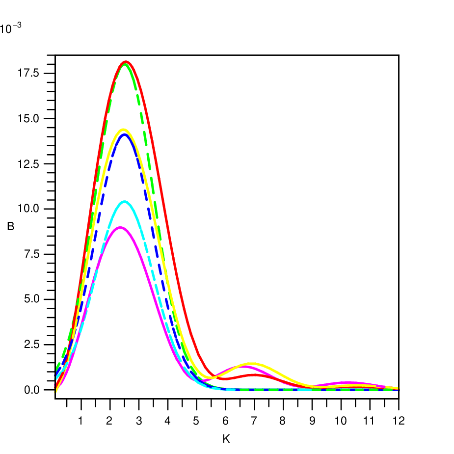
The last two equations are good fits to the real functions which are shown in Fig. 4. behaves as white noise for while . On small scales (large values of ) both and decay like . In the region where and are maximal, our approximations overestimate the real functions for values of (we will comment on this in Section 5.2). In the following analysis we will consider the maximal value of : for this value the approximations overestimate by about 16%.
The behaviour of and can be predicted from general considerations. First of all, the correlation function (30) vanishes for : the characteristic scale of the correlation function is the diameter of the bubbles. We therefore expect this scale to show up in the power spectrum at wave-number . This is indeed what happens, since the functions and change their behaviour at approximately . Moreover, since the correlation function is a function with compact support, its Fourier transform, the power spectrum, must be analytic in . We remind that an analytic function can be developed in power series around any point of its domain. The term of Eq. (3.2.1) is analytic for , if and only if and is an even integer . This justifies the white noise behaviour observed at large scales for . On the other hand, analyticity of the term for is satisfied if and only if with an even integer and . This justifies why increases as at large scales.

3.2.2 Unequal time correlation function
Up to now we have evaluated the velocity correlation function at equal times. We note however, from Eq. (21), that we actually need the correlation function evaluated at different (comoving) times , . The velocity in point at time can be correlated with the velocity in point at time . Consider, for example, . In this case, the unequal time correlation function is not zero if the velocity shell in the bubble includes at time , and grows to include at time . According to the approach outlined above, evaluating the correlation function at different times means performing the volume integral of Eq. (30) within regions given by the intersection of spheres of different radii (cf. Fig. 3). This integral is too complicated to be done analytically: therefore, within our analytical approach, we first try to simply approximate the unequal time correlation function with the one at equal time calculated in the previous subsection. This is a reasonable approximation, provided that the region of non-zero velocity at overlaps with the region of non-zero velocity at . If this is not the case, we simply set the unequal time correlation function to zero.
Reintroducing as the time of nucleation we find that, in the limiting case, the inner boundary of the non-zero velocity shell in the bubble at time equals the outer boundary at time if , where we remind that . Symmetrizing among the two times, we have then
| (48) | |||||
where is the Heaviside function. We choose arbitrarily to set the time appearing in the equal time correlator corresponding to the smaller of the two times.
In Section 5, we derive the gravitational wave spectra obtained using this approximate form of the unequal time correlation function and discuss its shortcomings. We will eventually propose another method, which consists in giving an approximate form directly for the unequal time anisotropic stress power spectrum, rather than for the velocity correlation function. As we will see, proceeding in this way we can have better control over the positivity of the power spectrum, and obtain more reliable results.
3.3 Anisotropic stress power spectrum: calculation
We now have everything we need to evaluate the anisotropic stress power spectrum of our source, using Eq. (24).
The unequal time correlation function Eq. (48), together with the equal time velocity power spectrum given in Eq. (40), lead to
| (49) |
with , , , and . Using the functions and given in Eqs. (3.2.1, 3.2.1), we can perform the above integral. A good approximation to the integral, after factorizing out the -dependence as , is given by
| (50) |
This fit, together with the exact integral, is shown in Fig. 5. The function is flat on large scales and changes slope at . A white noise behavior at large scales is expected, since the anisotropic stress power spectrum is the convolution of the velocity power spectrum: this simply means that the anisotropic stress is not correlated at distances larger than the source correlation scale . In Appendix C, we derive this in details. As one sees in Fig. 5, Eq. (50) is a very good approximation to the numerical integral. On small scales the convolution decays like and , hence like . This can be understood as follows: when , where denotes the wave number at which and peak, the main contribution to the convolution integral comes from the region . The value of a typical term in this region is about , and the phase space volume is : hence we expect for and analogous for the contributions containing .
Before we are ready to insert the expression (49) for in Eq. (15) to evaluate the gravitational radiation power spectrum, we need to determine the time dependence of and .


4 Time dependence of the phase transition parameters
We now investigate the actual time dependence of some parameters introduced previously, such as the fraction of volume occupied by bubbles at time , , which we need in Eq. (31), or the bubble radius44 4 In this section we specify what we actually take for the bubble radius, and we will denote it by . We remind that, in the case of deflagrations, this does not coincide with , which is the position of the shock front, but with .. In this section we closely follow Ref. [33] in the modeling of the first order phase transition.
The rate of bubble nucleation of the broken phase bubbles is defined as , where is the energy scale of the phase transition and the tunneling action. We Taylor expand the action at first order around a fixed time : the time at which the transition ends. Defining , one can rewrite the nucleation rate as . Note that we define in terms of comoving time, differently from the usual convention. The probability that a given point remains in the false vacuum at time is given by
| (51) |
where is the fraction of volume occupied by broken phase bubbles at time without considering bubble overlap [33, 39, 40]. Assuming that the universe remains static for the entire duration of the phase transition, and assuming a constant velocity for the bubble expansion , is simply given by
| (52) |
The quantity in Eq. (31) is given by . The times and are defined such that and . Following [33, 19], we choose a number and define as , so that . In the same way, we choose a number such that and . This gives the duration of the phase transition
| (53) |
In order to evaluate the mean bubble radius, we consider the number of bubbles which have a given radius at time . Calling the nucleation time of a bubble with radius at time , one has:
| (54) |
The shape of this distribution is shown in Fig. 5 of Ref. [33]. For each , it has a maximum at the value : this value defines the mean radius of the bubbles at time . Calling the time at which , so that , we set
The condition defines .
As already explained in Sec. 3.2, bubbles can be treated as combustion fronts moving at constant velocity only at times much later than nucleation time. Therefore, we identify in the evaluation of the emitted gravitational radiation. This leads to . We further decide to neglect the logarithms and simply set
| (57) | |||||
| (58) |
If we do not neglect the logarithms, we have to replace the final bubble size by . Neglecting the logs, we identify the duration of the phase transition with , and the radius of the bubbles at time with its mean value . We do not account for the possibility of having bubbles of different sizes at a given time.
5 Evaluation of the gravitational wave spectrum
We now want to evaluate the gravitational wave energy density per logarithmic frequency interval (6), which is given in terms of the GW power spectrum (15). According to Eq. (15), the latter evolves as ; however, this behavior is strictly valid only in a radiation dominated universe with a constant number of relativistic degrees of freedom (c.f. Sec. 2) and thus lacks generality. To estimate the GW power spectrum at , we therefore evaluate it at the end of the phase transition: , for which no assumptions have been made concerning the number of relativistic degrees of freedom. Then, we simply use its radiation-like evolution:
| (59) |
From Eqs. (6) and (15), reminding that we have
| (60) | |||||
| (61) |
where in the last equality we have set . In the above equation, we further have to substitute expression (49) for the anisotropic stress source. As already discussed in Sec. 2, since the source is active for an amount of time much shorter than one Hubble time, we neglect the expansion of the universe while gravitational waves are produced. Therefore, in Eq. (49) we set the enthalpy density to a constant, denoted by . Moreover, we eliminate the time dependence of the factors by substituting with the constant fluid velocity , corresponding to the fluid velocity of the inner boundary of the shell (cf. Eq. (3.2) and Fig. 2), remembering that . We explain the reasons for this choice below. We remind that the double integration in Eq. (61) is in time, with the notation , . With given in Eq. (50), we finally obtain using Eq. (59)
| (62) |
Let us first investigate the pre-factor in the above expression. The enthalpy density is
| (63) |
where denotes the radiation energy density in the universe, and denote the effective number of relativistic degrees of freedom today and at the time of the phase transition respectively. We also define a dimensionless parameter estimating the amount of kinetic energy present in the source, with respect to the radiation energy density. From the definition (17) of the energy-momentum tensor:
| (64) | |||||
| (65) |
We have chosen to define the above parameter in terms of the fluid velocity at the inner boundary of the velocity shell , which always satisfies both for detonations and deflagrations. This ensures that to remain consistent with an isotropic FRW universe.
Summarizing, we can rearrange the pre-factor in Eq. (62) in terms of the above defined parameters, of the conformal Hubble factor and of , as:
| (66) |
The gravitational wave energy density is therefore proportional to the square of the kinetic energy density of the source, as one would expect.
In the double integral of Eq. (62), we define the new integration variable , and the new dimensionless parameter
| (67) |
Following the discussion in Sec. 4, the function becomes
| (68) |
We finally obtain for the gravitational wave energy density spectrum today
| (69) | |||||
We recover the known result, that the amplitude of the gravitational wave spectrum is proportional to the square of the ratio between the duration of the phase transition and the Hubble time, [4, 41]. If the parameter , this means that the fluid motions vanish everywhere, and therefore no gravitational radiation is produced. The divergence in is only apparent, due to our definition of the kinetic energy density parameter in Eq. (65).
Expression (69) gives in all generality the power spectrum of gravitational radiation produced by spherically symmetric, stochastic configurations of fluid motions (such as broken phase bubbles in a phase transition), characterized by a velocity distribution which increases linearly in a shell of inner radius and outer radius . The integral determines the shape of the spectrum, and depends on the values of and of the velocity . These parameters should be chosen according to the physical situation under consideration.
We expect the large scale part of the GW spectrum to increase as . As explained in details in Appendix C, this is a simple consequence of the fact that the source has a finite correlation scale (corresponding in our case to the length-scale ). It is therefore a generic behaviour for causal sources. Conversely, the small scale part of the spectrum depends on the details of the source correlation function. This part of the spectrum is in principle affected by our choice of a linear growth for the velocity profile in the non-zero velocity shell (cf. Sec. 3.2). If we could account for the correct velocity profile, the power law dependence of the GW power spectrum at large might be different from what we find. On the other hand, the frequency at which the GW power spectrum peaks can again be predicted by general considerations. In fact, the velocity power spectrum given in Eq. (40) has a characteristic wave-number corresponding to the bubble diameter, . Also the anisotropic stress power spectrum changes slope at about . For the gravitational radiation power spectrum we therefore expect a peak at approximatively the same wave-number given by the mean bubble size at the end of the phase transition.
5.1 Unequal time approximations
The expression (69) has been derived using the approximation Eq. (48) for the unequal time correlation function of the velocity field. Under this approximation, the anisotropic stress power spectrum at different times takes the form given in Eq. (49), which has been substituted in Eq. (61) in order to evaluate the GW power spectrum. According to the definition of the GW spectrum , the time integral appearing in Eq. (61) should give a positive result. Therefore, the unequal time anisotropic stress power spectrum should be, by definition, a positive kernel, such that
| (70) |
where generically denotes the Green function of the wave equation (9). Even though the approximated form for the unequal time correlation function for the velocity field Eq. (48) seems reasonable from a physical point of view, it does not lead to a positive kernel for as it should. Expression (69) is not always positive and therefore it is unacceptable. To avoid this problem, we now define approximations directly for the unequal time correlator which are positive by construction. We first discuss two cases which are physically less motivated, but are very useful for comparison: the completely incoherent and completely coherent approximations. Finally, we discuss a third and better motivated approximation for that still gives a positive result. We believe that this last approximation is the one that best recovers the true result. Apart from being strictly positive, it has the advantage to be very close to the physically motivated approximation for the unequal time correlators of the velocity field. As we shall see, the peak position of the GW spectra is very similar in all cases, while the peak amplitude varies by up to one order of magnitude.
We consider first a totally incoherent source, that is uncorrelated for unequal times . We take the Ansatz (cf. Eq. 49)
| (71) | |||
| (72) |
We multiply the - function by the characteristic time in order to maintain the correct dimensions. Under this assumption, the oscillating term in Eq. (61), , integrated with the delta function, becomes simply 1 and we recover a positive result. Using the same notations as in Eq. (69), the GW spectrum from totally incoherent bubbles is (see Fig. 6)
| (73) | |||||
The opposite situation is given by a totally coherent source, that is correlated for every time and . In this case, the Ansatz for the anisotropic stress power spectrum is
| (74) |
We rewrite the oscillating term using the duplication formula. This allows us to split the double integral into a sum of two positive terms. The GW spectrum is in this case (see Fig. 6)
| (75) | |||||
The positive part of the result based on the approximated unequal time correlation function for the velocity field, is in between these two extreme cases: the Heaviside functions introduce correlation only among times and which are sufficiently close to each other. We therefore expect also the correct result for the GW spectrum to be in between the limiting cases described above. Moreover, for sufficiently large scales the details of the time correlation do not matter, and we expect that the GW spectra derived using these different approximations become comparable at these scales. As we will see below, this is indeed the case (c.f. Fig. 6).
Finally we introduce top-hat unequal time correlations directly in the anisotropic stress power spectrum, rather than in the velocity correlation function. This approximation is also an intermediate case between the completely coherent and incoherent ones, and it is constructed to always give a positive result for the GW power spectrum as we will discuss. We make the following symmetric Ansatz:
| (76) | |||||
| (77) |
Under this assumption, we set the correlation to zero for modes with a time separation larger than , where is a positive, dimensionless parameter of order unity (to be specified later). Therefore, the anisotropic stresses at different times are correlated if the time separation is less than about one wavelength. Physically, this just means that longer wavelengths are correlated over a longer time. This corrects the lack of correlation that resulted from our very first approximation. The GW power spectrum becomes:
| (78) | |||
which is apparently positive for . Resolving the Heaviside functions, we have to consider two separate cases. For we find the spectrum (see Fig. 6)
| (79) |
and for we find
| (80) |
The GW spectrum remains positive for since in the range , , and in the range , both and are positive. In the limit the result tends to zero. A reasonable value is . In Fig. 7 we show how the power spectrum depends on the value of . We now present the results obtained for the different approximations discussed above, in the cases of detonations and deflagrations.
5.2 GW from detonations
As explained in Sec. 3.2, in the case of detonations is the outer radius of the bubbles. Therefore, . We restrict ourselves to the case of Jouguet detonations, so that . The value of the bubble wall velocity in Jouguet detonations is given in Refs. [34, 20] in terms of the ratio
| (81) |
where denotes the radiation energy density in the universe:
| (82) |
The outer maximal fluid velocity is given by the Lorentz transformation (see Eq. 25)
| (83) |
where for the last equality we have substituted (82) and . Moreover, the parameter takes the form
| (84) |
For detonations55 5 To be in the detonation regime means that there is essentially no friction. In other words, interactions between the bubble wall (the Higgs field) and the particles in the thermal bath can be neglected. This is a strong assumption which can work if the released latent heat is indeed very large. Model-independent studies (such as Ref. [25]) have used Eq. (82) for the bubble wall velocity. However, when considering a particular model, one should compute friction effects and therefore derive a more realistic value for the bubble wall velocity, following for instance the procedure of Ref. [42]. This requires to compute the bubble wall profile. , it is therefore sufficient to specify , and all the quantities necessary to evaluate the integrals in Eqs. (69,73,75,79,80) are determined. Knowing in addition the duration of the phase transition fully determines the gravitational wave signal. We choose a broad range of values for : . corresponds to . As discussed in section 3.2.1, for our approximations for the velocity power spectrum overestimate the true result by about 16%.

Let us first discuss the shape of the spectrum. We have four different approximations for the unequal time correlator: the top-hat unequal time correlator for the velocity field in real space, Eq. (69), the incoherent case Eq. (73), the coherent case Eq. (75), and the top-hat unequal time correlator for the anisotropic stress in Fourier space, Eqs. (79,80). They give rise to comparable spectra. In Fig. 6 we show the result of the integrals as a function of . We have fixed the values and . The spectra increase like at large scales, and have comparable amplitudes. This is expected, since the details of the time correlations should not matter at sufficiently large scales and the source is uncorrelated in real space (cf. Appendix C). Also, the positions of the peak approximatively coincide in the four cases, and correspond to , so . This is comparable to the peak of the anisotropic stress power spectrum , due to the fact that GW production accounts for the full evolution of the bubbles, and for all times . The peak of the GW spectrum is independent of time and corresponds to the mean bubble radius at the final stages of the phase transition, close to . The amplitude at the peak is roughly the same for the two top-hat approximations and for the coherent case, with the value of the integral at the peak of the order of . Within the precision of our analytical evaluation this difference is negligible. On the other hand, the incoherent case overestimates the amplitude by a factor 5. The small scale part of the spectrum is also different in the incoherent case with respect to the others: it decays slower, as as opposed to with . The reason for this behaviour is apparent by looking at the integral in Eq. (73): once has overcome the value at which the integrand peaks, the contribution from the integral becomes small and the function decays nearly like . Conversely, in the cases of Eqs. (75,79,80), at sufficiently large scales the spectrum scales nearly like . We explain the small scale decay on the basis of dimensional arguments in Appendix C. The two top-hat approximations are in very good agreement up to . For larger , the spectrum obtained for the top-hat in the velocity correlation becomes negative. This is due to the contribution from the first integral in Eq. (69), which is negative after . Its absolute value is between the totally coherent approximation and the top-hat in wave-number approximation. We consider the top-hat in wave-number ansatz which is given in Eqs. (79,80) to be the best approximation for the unequal time correlators.


In the top left panel of Fig. 7 we show that the integral of Eqs. (79,80) is only weakly dependent on . The parameter plays a greater role in determining the overall amplitude of the GW signal (which will be discussed later on). On the other hand, the shape of the spectrum depends significantly on the choice of once approaches . We remind that defines the time interval beyond which the correlator of the anistropic stress tensor vanishes. In the top right panel of Fig. 7 we fix and vary . Values of around the peak correspond to the region , where the result is dominated, for a wide range of values of , by the first integral in Eq. (80). The pre-factor of this integral decays like at high enough values of . This is roughly the decay we see in Fig. 7 for low . When becomes very close to , the factor multiplying the first integral in Eq. (80) becomes so small that the contribution from the second integral in (80) takes over. For high values of , the second integral decays much faster than . However, because of the integration limits, it is more and more suppressed as increases: therefore, at some given value, the first integral takes over again and the spectrum decays roughly like . More precisely we find a decay at large . This behavior is reached for higher and higher values of as approaches , as is shown in Fig. 7. For our final results, we choose the value . This may underestimate the signal somewhat at high frequencies compared to values , but this is a reasonable conservative choice. Values still closer to , would be unjustifiably fine-tuned.
The following approximate gravitational wave power spectrum is fairly general. We chose but as shown in Fig. 7, the shape of the spectrum is almost insensitive to the value of ; the dependence is essentially only in the prefactor and implicitly in :
(85)
This approximation for int is shown in the lower panel of Fig. 7, and we remind that is defined as a function of and in Eq. (65).


Let us now investigate the overall amplitude of the signal at the peak frequency.
| (86) |
where the factor accounts for the contribution of the integral at the peak frequency (cf. low panel of Fig. 7). In order for the bubbles to percolate and convert the entire universe to the broken phase, the phase transition must occur much faster than one Hubble time. We study the values of . Since the velocity of the bubbles is fully determined by the parameter , so is the fluid velocity and, in turn, the factor and the mean kinetic energy parameter , see Eqs. (82,83,84). We plot and as a function of in Fig. 8. Specifying and fully determines the amplitude. Substituting in (86), and setting , we find:
| (87) |
which we plot in Fig. 9.
The peak amplitude depends quadratically on the duration of the phase transition, and grows steeply (also roughly quadratically) with as long as . At the dependence on becomes rather weak, since the bubble velocity approaches its maximum, . The maximum gravity wave density parameter which can be achieved by bubble collisions in a strongly first order phase transition , and is of the order of . Note that our approximations break down for smaller values of , since we have neglected the factor so that becomes the duration of the phase transition which must be significantly smaller than a Hubble time.
5.3 GW from deflagrations
In the case of deflagrations, coincides with the shock front of the shock wave taking place in the symmetric phase. Therefore, we set . The inner radius is the bubble wall, so that . The fluid velocity is given by
| (88) |
where is the incoming velocity of the symmetric phase fluid into the front, in the rest frame of the discontinuity.
In order to estimate the gravitational wave production, we follow the analysis of deflagrations presented in Appendix A of Ref. [20]. There, the authors numerically integrate the energy-momentum conservation equations at the deflagration front with different initial conditions. The velocity profile they find is in principle different both from the constant one occurring in planar deflagrations, and from the linear one that we took in our simplified analysis. However, we choose two different cases which they have analyzed, for which the deflagration is quite strong and the velocity profile is actually almost constant. In the first case, they set and , and find (and consequently ). In the second case, close to Jouguet deflagrations, they set and , and find (and consequently ). The velocity profiles for these values are shown in Fig. 9 of [20]. Since in the case of deflagrations there is no simple relation among the velocity of the shock front and the parameter denoting the strength of the phase transition, we simply leave as a free parameter in our analysis, for which we take the two values given above.
The analysis of the shape of the spectrum is on the same footing as for detonations. The results of the unequal time correlator for the anisotropic stress are shown in Fig. 10 for fixed values of and . The results for the incoherent and top-hat in the anisotropic stress cases are similar to the case of detonation. We recover the expected behaviour at large scales, and the amplitudes are comparable at low wave number. The peak is located at , corresponding to . On the other hand, the coherent and top-hat in the velocity correlation cases are slightly different in the high frequency range, because the frequency of the oscillations is increased, due both to the smaller value of , and to the smaller value of . These parameters in fact appear in the arguments of the Green functions in Eq. (69) and (75). In the region where the power spectrum becomes negative, in the top hat in velocity case, the solution is no longer reliable. We therefore discard it and take as best approximation the unequal time correlator of the anisotropic stress power spectrum, as we did for detonations.


The result of Eqs. (79,80) is very weakly dependent on the value of the velocity . This is analogous to the weak dependence on found for detonations. We do not display this dependence as it is very similar to the top left panel of Fig. 7 where the role of is played by which is varied between 0.59 and 0.73. Correspondingly, when varying , we obtain a dependence similar to the one shown in Fig. 7. For fixed and we can approximate the result as follows:
(89)
This is essentially identical to Eq. (85) except for the values of and in : In the case of deflagrations we cannot reduce the dependence exclusively to the two parameters and , since no direct relation between the velocities of the shock front, the velocity of the bubble wall and the strength of the phase transition is known in general. In this case, the velocity of the shock front is expected to depend also on the properties of the ambient plasma, like friction, and not only on the strength of the phase transition determined by . The amplitude at the peak frequency is the same as the detonation formula (86) except that 0.084 is replaced by 0.050. This factor accounts for the contribution of the integral at the peak frequency (cf. Fig. 10):
| (90) |
The first plot of Fig. 11 shows as a function of the fluid velocity for two values of , corresponding to the cases analyzed in [20]. Obviously, the value of is in principle fixed once , and are given; however, the relation among these parameters is not known explicitly. Therefore, we have decided to keep as a free parameter. The fluid velocity induces the biggest variation in the amplitude of the signal, and is therefore the most relevant parameter determining . This appears clearly in the second plot of Fig. 11, where we show the amplitude of the GW signal Eq. (90) as a function of , for the same two values of and varying . The dependence on is negligible compared to the dependence on .
6 Some comments on our approach
In numerical simulations, the stochastic background of GWs arises from averaging over several deterministic realizations of bubble collisions. In our approach instead, to account for the intrinsic randomness of the nucleation process, we define the bubble velocity as a random variable. The source of the stochastic background of GWs is the tensor part of the anisotropic stress of the stochastic, homogeneous and isotropic velocity field.
The calculation of the velocity correlation function in Sec. 3.2.1 implicitly assumes that the bubbles, and consequently the velocity configuration, are all independent from each other: the velocity correlation function is different from zero only if the points and are in the same bubble. Therefore, one may wonder in which sense this procedure is a model of bubble collisions. Indeed, in our model the only non-vanishing correlation coming from a (possibly) collided region is given by the sum of correlations from two independent bubbles: for every and we can find a bubble center position such that a bubble encompasses the two points, giving a non-zero result, provided that the probability to find a center in that position is not zero. This is accounted for by multiplying the correlation with the probability that a given point is in the broken phase at a given time, cf. Eq. (30).
Therefore, even though we do not model in a deterministic way the resulting velocity field from the collision of bubbles, we do account for their overlap; it is the overlap from several bubbles which gives us a non-zero correlation function for the tensor part of the anisotropic stress, as opposed to the spherically symmetric situation described in Appendix A. The anisotropic stress correlation function, in fact, involves the four-point correlation function of the velocity field, cf. Eq. (19). This quantity, in contrast with the two-point correlation function, is non-zero also for points and belonging to different bubbles66 6 .. In other words, when we calculate the two-point correlation function of the velocity field Eq. (30), we break spherical symmetry since every point in space becomes equivalent to another and there is no longer a center of symmetry. The center of symmetry has become a random variable, and we average over all its possible positions. Using the ergodic theorem, this is equivalent to an average over several realizations for the center positions, i.e. several realizations of the nucleation process, i.e. several realizations of the velocity field distribution. In this way, we account for the overlap of several bubbles, which breaks spherical symmetry and leads to a non-zero power spectrum of the tensor anisotropic stress, generating gravitational radiation.
7 Summary
Since the GW signal from bubble collisions was already evaluated in Refs. [18, 17, 19, 20], in this section we gather our final formulas and compare them with the ones given so far in the literature. We conform to the notation used previously, for the comparison to be straightforward. The relevant formulas are compiled for instance in Ref. [24]: there, Eq. (4) gives the frequency at which the GW spectrum peaks and Eq. (5) shows the dependence of the amplitude of the GW signal at the peak frequency on the relevant parameters of the bubbles evolution. These formulas are valid in the case of Jouguet detonations, and do not show how the GW spectrum depends on other than the peak frequency. Before proceeding with the comparison, we recap the main assumptions in our calculation: 1) we assume radiation domination; 2) the fluid velocity profile inside the bubble is linear; 3) is our stochastic variable via the bubble center as we average over all possible positions of the bubble center. Therefore, we do not model collisions in a deterministic way. We rather account for all possible configurations of the velocity field which include the case where bubbles overlap, even though we use the velocity profiles of uncollided bubbles; 4) we use the Wick theorem to express the 4-point correlation function in terms of the 2-point correlation function, even if the velocity is presumably not a gaussian random variable; 5) all bubbles have the same size ; 6) we use the top hat approximation for the correlator of the anisotropic stress tensor at different times; 7) the enthalpy and the Lorentz factor do not depend on .
Using the notation
| (91) |
from the results given in Section 5.2, Eqs. (85, 86) and Section 5.3, Eqs. (89, 90), we find that increases at small as (compared to in Kosowsky et al. [17]), and at large it scales as (as in Kosowsky et al). The full spectrum is given by
(92) (93)
Let us first discuss the peak frequency. It is given by
| (94) |
| (95) |
We remind that in our notations expresses the duration of the phase transition: bubbles are generated at the beginning of the phase transition and collide after a time given approximately by . We have in fact set to 1 the logarithm relating and , c.f. Eq. (53) of section 4 (this logarithm can be easily inserted in all the following equations: it will introduce a multiplying factor in the ratio and will also change the value of the integral (69)). Moreover, corresponds to either the characteristic bubble velocity (in detonations) or the shock wave velocity (in deflagrations). The characteristic frequency at the time of emission is . As expected, it is associated with the maximal size of the spherical fluid velocity configuration which generates the GW signal. This can be either the bubble itself, in the case of detonations, or the spherical shock front preceding the bubble, in the case of deflagrations. Since , the peak frequency for detonations is smaller than that for deflagrations (the size of the velocity configuration is bigger). Using and , we can rewrite the peak frequency as
| (96) |
| (97) |
where of course .
The above peak frequency is bigger than the one in Refs. [20, 24] by a factor . The factor , that shifts the peak to higher frequencies for low velocities, is absent in [20, 24], and is related to the fact that the characteristic frequency we find is determined by the size of the bubbles instead of the duration of the phase transition [4]. The property of causality of the source directly determines this characteristic frequency. Since the source is causal, the velocity correlation function goes to zero at the length-scale corresponding to the size of the bubbles. The same length-scale determines the peak in the velocity power spectrum, and from there it is transferred to the GW power spectrum (c.f. also the discussion in Ref. [43], where it is explained that gravity waves emitted during short cosmological events such as phase transitions typically inherit the wave number and not the frequency of the source) 77 7 Note that, being in a cosmological context, we do not perform a time Fourier transform of the energy momentum tensor in contrast to Eq. (23) of Ref. [20]. In [20] the authors assume that “the frequency dependence of the spectrum is set by the timescale ” (as written before eq. (28) of [20]). Our finding, on the other hand, is that the frequency dependence of the spectrum is set by the bubble size . Since in the detonation regime approaches 1, in the simulations of Ref. [20] one does not really see this difference..
The factor , instead, comes from the details of our modeling of the source. It follows from the factor 4.5 in Eq. (94) (see Fig. 6 and Fig. 9 and discussion thereafter). We found that the velocity power spectrum has a characteristic wave number , corresponding quite well to that coming from the bubble diameter . The time-dependent anisotropic stress power spectrum instead changes slope around (see Fig. 5). The characteristic wave number of the GW spectrum is associated to , the typical radius of bubbles at the end of the phase transition when bubbles collide, and is found to be . This differs from the value obtained in Kamionkowski et al. (see Fig. 7 of Ref. [20] and the associated uncertainty). For , GeV and , corresponding to a typical (first order) electroweak phase transition, we find to be compared with LISA’s peak sensitivity which is estimated to be 2 mHz. The increase in the peak frequency that we obtain relative to Ref. [20] is actually welcome for probing the electroweak phase transition with LISA88 8 This result should be taken with caution, see the “Note added” at the end of this Section..
Let us now discuss the peak amplitude. A simple order of magnitude estimate shows how the result depends on the duration and the energy density of the source. From the perturbed Einstein’s equations , one gets the following order of magnitude estimate for the amplitude of the tensor perturbation (we drop indices for simplicity):
| (98) |
where we inserted as the characteristic time on which the perturbation is evolving, and denotes the energy momentum tensor of the source. From Eq. (17) and definition (65), we can write
| (99) |
We want to estimate the energy density in gravitational waves, defined in Eq. (3). The above equation (98) suggests that , and so we obtain
| (100) |
Substituting Friedmann equation in the radiation dominated era , and considering that the GW energy density evolves like radiation, we obtain for the GW energy density today the simple expression
| (101) |
This shows that the GW energy density scales like the square of the ratio between the time duration of the source and the Hubble time, and the square of the energy density in the source.
More precisely, from Eqs. (86,90) we get the following result:
| (102) |
where 0.084 is replaced by 0.050 for deflagrations, and
| (103) |
with :
| for Jouguet detonations, | (104) | ||||
| for deflagrations. | (105) |
There is no simple analytic relation between , and in the case of deflagrations. For detonations, is given above, taken from Refs. [34, 20]. Using and we find the peak amplitude:
| (106) |
| (107) |
where 9.8 is replaced by 5.8 for deflagrations. The signal vanishes if the fluid velocity is zero. It also vanishes when the shell’s thickness is zero (), this happens if (corresponding to ) for detonations and for for deflagrations. Our result is to be compared with the expression reported in Eq. (5) of Ref. [24], which is only valid for Jouguet detonations:
| (108) |
Here
is the parameter defined in Eq. (22) of
Ref. [20], denoting the fraction of vacuum
energy which goes into kinetic energy of the fluid (rather than
thermal energy). Therefore, the combination is
equivalent in our notation to the parameter . The
above expression for is a fitting formula that the
authors of [20] determined by integrating
numerically the energy momentum tensor of the velocity profile
corresponding to a Jouguet detonation, for different values of
. On the other hand, we have defined in terms of the fluid velocity at the
inner boundary of the velocity shell, starting from the approximated
velocity profile given Eq. (3.2). As it should be, the
dependence on of the two parameters is comparable, see
Fig. 12 where we used , and
. In
Fig. 13, we show the comparison between our peak
amplitude (107) and the result used in
[24] (Eq. 108).


In summary, our amplitude for the signal is comparable (but can differ by one order of magnitude for some values of the parameters) to the one obtained with an inherently different method, that of numerical simulations in the envelope approximation [18, 17, 19, 20]. This confirms that the details of the collision’s modeling are not so crucial and what really matters at the end is the size of the velocities involved in the process. Note also that we computed the GW energy density spectrum without using the Weinberg formula i.e. without making the wave zone approximation. The latter assumes that the observer is at a distance much larger than the dimension of the source, while our source is spread over the entire universe.
Kamionkowski et al. obtain a non-vanishing signal in the limit of vanishing thickness. This can be understood as follows. In Ref. [17, 18, 19], they first study bubble collisions taking place in vacuum, so that the source of GW was the energy momentum tensor of the scalar field: being given by the spatial gradient of the scalar field, this is non-zero only at the bubble wall. In their later work Ref. [20], they consider bubble collisions in a thermal bath and in this case they use as the GW source the energy-momentum tensor of the relativistic fluid rather than that of the scalar field. Nevertheless, they keep using the envelope approximation. This is why they obtain a large signal even if the shell of fluid velocity has vanishing thickness. In contrast, by construction, there is no signal in this limit in our model, meaning that the kinetic energy of the fluid (which is our only source as we did not include the gradient energy of the scalar field) is different from zero only over a finite volume. On the other hand, we can extrapolate our results to the deflagration regime. Typically, for the detonation case, in the limit Ref. [20] finds a non-zero GW signal, since in the envelope approximation this is just the lower bound of the bubble wall velocity. Within our model, in this limit, the thickness of the non-zero velocity shell goes to zero and the GW signal as well; however, this only shows the break down of the detonation regime, and the necessity of treating the problem in the deflagration approach.
In Figure 14, we plot the peak amplitude as a function of the maximal fluid velocity . In contrast with the case of Jouguet detonations, for deflagrations, we cannot express the signal as a function of only. Indeed, for small velocities, the relation between and the bubble velocity will depend on the interactions between the bubble wall (the Higgs field) and the particles in the thermal bath. In any given model of a first-order phase transition, one can in principle compute the bubble wall velocity and the consequent fluid velocity profile, see e.g. Ref. [42] for the case of a weakly first-order EW phase transition, and Ref. [44] for the strongly first-order phase transition presented in Ref. [6]. Provided that the released latent heat is large, one can obtain a large bubble wall velocity. In addition, one would have to look carefully at the physics of deflagrations to derive the relation between the fluid velocity and that of the bubble wall, see for instance Ref. [35].
To conclude, our main new results can be summarized as follows:
- •
Our description applies to both detonation and deflagration (the fluid velocity is non-zero over a finite volume rather than on an infinitely thin wall and ).
- •
Our peak frequency is parametrically larger ().
- •
We provide an analytic expression for the shape of the spectrum.
The possibility that the signals discussed here, if they are produced at the electroweak phase transition, could be detected with LISA will be discussed in an upcoming publication [29]. We confirm that the GW signal coming just from bubble collisions is observable only for very large fluid velocities. Indeed, LISA’s best sensitivity is not much below . Such a value can be reached if and . More realistic values would require in order to lead to an observable signal. As mentioned in the introduction and as will be presented in [29], there are other sources (magnetic field and turbulence) of GW during phase transitions and the signal from bubble collisions is just one contribution.
Note added
Our results for the position of the peak and the slope of the spectrum at large frequencies strongly depend on the time structure of the anisotropic stress. In our modelization, it grows with time and is suddenly switched off at the end of the transition. This discontinuity is somehow unphysical. Indeed, our Eq. 31 does not take into account the fact that towards the end of the transition, there is no more intersecting region but only one single bubble. As discussed in details in [45], if the source is switched off smoothly and we consider the coherent case as indicated by numerical simulations [46] and if the relevant correlation length is taken to be the size of the uncollided region rather than the bubble size, then the peak position does not depend on the velocity and is given by . Besides, numerical simulations [46] which are carried out under the thin-wall approximation also indicate that the slope of the spectrum at high frequencies typically scales as .
Acknowledgments
We thank Riccardo Sturani for reading the manuscript. CC and RD acknowledge support by the Swiss National Science Foundation.
Appendix A One single bubble
If there was only one bubble, there would not be any gravitational radiation since a single bubble corresponds to a spherically symmetric distribution of energy and momentum which cannot emit gravitational waves. In this Appendix we show that the anisotropic stress from a single bubble is purely scalar: this means that there exists a function such that
| (109) |
where denotes the energy momentum tensor of a bubble. Such a scalar component is projected out by the tensor projection operator which is given in Fourier space in Eq. (8), and does therefore not contribute. In this case, from the above equation the function must satisfy the condition
| (110) |
We now demonstrate that this condition is always satisfied for a single, spherically symmetric bubble. For one spherically symmetric bubble we have, up to the constant enthalpy ,
| (111) | |||||
| (112) | |||||
| (113) | |||||
| (114) |
For the third equal sign we have used spherical symmetry, we work with the Ansatz , and the prime denotes the derivative w.r.t. . On the other hand, for a spherically symmetric function we have
Therefore, if we find a function which satisfies
or, equivalently
| (115) |
the anisotropic stress (111) is equal to the expression given in Eq. (109), therefore, it is a pure scalar. This is indeed the case, since Eq. (115) is an ordinary linear differential equation which always has a solution for a given radial velocity .
Hence a single spherically symmetric bubble only generates scalar perturbations and does not contribute to the tensorial part of the energy momentum tensor , which is the source of gravity waves. This is of course not surprising given that spherically symmetric configurations only have scalar degrees of freedom. Nevertheless, we have added this brief calculation here since one might draw wrong conclusions from the fact that the anisotropic stress of a single, spherically symmetric bubble does not vanish.
Another way to arrive at the same result is to show that the tensor projection operator given in Eq. (8),
| (116) | |||||
| (117) |
vanishes when applied to a spherically symmetric stress tensor. For a single bubble one has then
Appendix B Calculation of the velocity field power spectrum
In this appendix we explain how to evaluate the velocity correlation function Eq. (30) and Fourier transform it to obtain the velocity power spectrum Eq. (40). The quantity we need to calculate is the tensor
| (118) |
The intersection volume varies with the distance between and , as shown in Fig. 3, with . We choose an orthonormal basis with . One identifies four different regions: setting , they are given by the limiting values
| (119) |
The intersection volume is symmetric under rotations around , so in order to perform the integral in (118) we choose cylindrical coordinates with and . We have
| (120) |
Substituting the above formulas in (118) and performing the integration in , one sees that, because of cylindrical symmetry, the tensor is diagonal. Evaluating (118) reduces simply to calculate the two integrals
| (121) |
The limits of integration, here generically denoted with , depend in fact on the variable . As an example, in the region , the first integral becomes:
Analogous expressions can be found for the remaining three regions, and similarly for . The final result of the integrations are the two continuous functions and , as a function of the variable , which are too long expressions to be written explicitly here.
Knowing and , we impose the condition of statistical homogeneity and isotropy for the velocity field, meaning that we impose the tensorial structure
| (122) |
where the second equality is a straightforward consequence of our choice . The two-point correlation function for the velocity field takes the final form (cf. Eq. 34)
| (123) |
where the pre-factor is independent of and the volume is given in Eq. (32).
In order to know the power spectrum, we have to Fourier transform the above equation with respect to the variable . Because of homogeneity and isotropy, we get a delta function in momentum. We rewrite the Fourier transform of the second term in the sum, which is direction dependent, in terms of derivatives with respect to the wave vector, and we obtain:
| (124) |
The Fourier transform of a function only of gives a function only of wave number . Knowing this, we can re-express the partial derivatives, to obtain expression (36) and followings. The Fourier integrals, as for example
| (125) |
need to be further divided in the sum over the four integrals corresponding to the regions described above, depending on the value of , since in each of these regions the integrand takes a different form. Again, we do not write the complicated full expression of the result, for which we found the fitting formulas (3.2.1) and (3.2.1) shown in Fig. 4.
Appendix C Large and small scale part of the GW power spectrum
We have seen that the gravitational wave power spectrum, independently of the different time approximations, always grows like at scales larger than the peak scale . The reason for this general behaviour is that the source is uncorrelated at these scales: therefore, the power spectrum of the anisotropic stress source is simply the incoherent sum of uncorrelated regions, and is white noise. The white noise behaviour for the anisotropic stress in turn determines the increase for the GW power spectrum.
On the other hand, we also saw that for the small scale part of the spectrum we always recover roughly a decrease, with the only exception of the completely incoherent case (cf. Eqs. (71,73)). The small scale decrease can be understood from dimensional arguments. In this Appendix we present general arguments for the origin of the above mentioned power laws for the large and small scale part of the GW power spectrum.
Let us first concentrate on the large scale limit. We start with a generic velocity power spectrum showing a peak at a characteristic scale . The scale , corresponding in our case to the bubble diameter , may depend on time. We assume that the large and small scale behaviors are given by two power laws,
satisfying the conditions , so that the energy density is dominated by the contribution at the peak. The pre-factor denotes the average energy per unit enthalpy of the source. For bubbles, we have for the function and for , cf. Eqs. (3.2.1,3.2.1) and the discussion thereafter (we will treat the small scale decrease of these functions later on). The anisotropic stress power spectrum is given by the convolution of the velocity power spectrum (cf. Eq. 24). Setting and , and neglecting angular dependencies, we have
| (129) |
In the large scale limit , in the second integral we can safely neglect with respect to and simply set . In the first integral we have to be a little more careful. If , the main contribution to the integral comes from the divergence at and the integral picks a behaviour . In our physical bubble situation, we have , ; we therefore choose to analyze only the case , for which we find:
| (130) |
Therefore, the anisotropic stress at large scales is white noise. Going back to Eqs. (6) and (15), we see that for a constant anisotropic stress power spectrum, the GW power spectrum behaves like
| (131) |
Here we have re-expressed the conformal time derivative appearing in Eq. (6) in terms of a derivative with respect to , and we have taken into account that converting the double integral over the Green function in Eq. (15) into a double integral with respect to conformal time, induces an additional factor . We therefore recover the observed large scale behavior .
We now turn to the small scale limit, . In this case, our fits to the functions and decrease like . As argued in Section 3.3, this power law is transferred to the small scale behaviour of the anisotropic stress power spectrum, cf. Eqs. (49,50), which takes the form
| (132) |
where decreases like for , and we neglect all the other time dependent factors, which are irrelevant for the argument presented here. Inserting the above expression in Eq. (15), one finds
| (133) |
where for the second equality we have used the fact that . Substituting the above formula into Eq. (6) rewritten in terms of the derivative with respect to , one finally obtains
| (134) |
where the double integral simply causes a modulation in the spectrum. We recover, in the large wave number limit, the decrease, which is a simple consequence of dimensional analysis since is a function of only in the relevant regime. This power law usually acquires small corrections due to the fact that the integral in Eq. (134) is not completely independent of . Depending on the approximation for the unequal time anisotropic stress power spectrum, we actually found power laws with in the range . Within our approximation, these may well also be logarithmic corrections to the slope .
In the case of the totally incoherent unequal time approximation, the argument is changed because of the delta function in time: the form of the anisotropic stress power spectrum is now (cf Eq. 71)
| (135) |
Repeating the above argument, one easily finds that the large wave number power law is now changed to ( with the corrections from the integral).
References
- [1] URL http://www.ligo.caltech.edu/
- [2] URL http://www.virgo.infn.it/
- [3] URL http://lisa.jpl.nasa.gov/
- [4] E. Witten, Phys. Rev. D 30, 272 (1984).
- [5] C. Hogan, MNRAS 218, 629 (1986).
- [6] C. Grojean, G. Servant and J. D. Wells, Phys. Rev. D 71, 036001 (2005) [arXiv:hep-ph/0407019].
- [7] A. Hebecker and J. March-Russell, Nucl. Phys. B 781, 99 (2007) [arXiv:hep-th/0607120].
- [8] L. Randall and R. Sundrum, Phys. Rev. Lett. 83, 3370 (1999) [arXiv:hep-ph/9905221].
- [9] P. Creminelli, A. Nicolis and R. Rattazzi, JHEP 0203, 051 (2002) [arXiv:hep-th/0107141].
- [10] L. Randall and G. Servant, JHEP 0705, 054 (2007) [arXiv:hep-ph/0607158].
- [11] B. Hassanain, J. March-Russell and M. Schvellinger, arXiv:0708.2060 [hep-th].
- [12] J. Kaplan, P. C. Schuster and N. Toro, arXiv:hep-ph/0609012.
- [13] G. Nardini, M. Quiros and A. Wulzer, JHEP 0709, 077 (2007) [arXiv:0706.3388 [hep-ph]].
- [14] X. Chen, R. Easther and E. A. Lim, JCAP 0706, 023 (2007) [arXiv:astro-ph/0611645]. R. Easther, J. T. Giblin and E. A. Lim, Phys. Rev. Lett. 99, 221301 (2007) [arXiv:astro-ph/0612294].
- [15] J. Garcia-Bellido, D. G. Figueroa and A. Sastre, arXiv:0707.0839 [hep-ph].
- [16] J. F. Dufaux, A. Bergman, G. N. Felder, L. Kofman and J. P. Uzan, arXiv:0707.0875 [astro-ph].
- [17] A. Kosowsky, M. S. Turner and R. Watkins, Phys. Rev. D 45, 4514 (1992).
- [18] A. Kosowsky, M. S. Turner and R. Watkins, Phys. Rev. Lett. 69, 2026 (1992).
- [19] A. Kosowsky and M. S. Turner, Phys. Rev. D 47, 4372 (1993) [arXiv:astro-ph/9211004].
- [20] M. Kamionkowski, A. Kosowsky and M. S. Turner, Phys. Rev. D 49, 2837 (1994) [arXiv:astro-ph/9310044].
- [21] A. Kosowsky, A. Mack and T. Kahniashvili, Phys. Rev. D 66, 024030 (2002) [arXiv:astro-ph/0111483].
- [22] A. D. Dolgov, D. Grasso and A. Nicolis, Phys. Rev. D 66, 103505 (2002) [arXiv:astro-ph/0206461].
- [23] R. Apreda, M. Maggiore, A. Nicolis and A. Riotto, Nucl. Phys. B 631, 342 (2002) [arXiv:gr-qc/0107033].
- [24] A. Nicolis, Class. Quant. Grav. 21, L27 (2004) [arXiv:gr-qc/0303084].
- [25] C. Grojean and G. Servant, Phys. Rev. D 75, 043507 (2007) [arXiv:hep-ph/0607107].
- [26] C. Caprini and R. Durrer, Phys. Rev. D 74, 063521 (2006) [arXiv:astro-ph/0603476].
- [27] G. Gogoberidze, T. Kahniashvili and A. Kosowsky, arXiv:0705.1733 [astro-ph].
- [28] T. Kahniashvili, G. Gogoberidze and B. Ratra, arXiv:0802.3524 [astro-ph].
- [29] C. Caprini, R. Durrer and G. Servant. To appear.
- [30] M. Maggiore, Phys. Rept. 331, 283 (2000) [arXiv:gr-qc/9909001].
- [31] D. N. Spergel et al. [WMAP Collaboration], Astrophys. J. Suppl. 148, 175 (2003) [arXiv:astro-ph/0302209].
- [32] A.H. Guth and E.J. Weinberg, Nucl. Phys. B212, 321 (1983)
- [33] M.S. Turner, E.J. Weinberg and L.M. Widrow, Phys. Rev. D46, 2384 (1992)
- [34] P. J. Steinhardt, Phys. Rev. D25, 2074 (1982).
- [35] J. Ignatius, K. Kajantie, H. Kurki-Suonio and M. Laine, Phys. Rev. D 49, 3854 (1994) [arXiv:astro-ph/9309059].
- [36] L.D. Landau and E.M. Lifshitz, Fluid Mechanics, Volume 6 of the Course of Theoretical Physics, Pergamon Press, New York, 1959
- [37] R. Courant and K.O. Friedrichs, Supersonic Flow and Shock Waves, Applied Mathematical Sciences, Volume 21, Springer-Verlag, New York, 1976
- [38] M. Laine, Phys. Rev. D 49, 3847 (1994) [arXiv:hep-ph/9309242].
- [39] A.H. Guth and E.J. Weinberg, Phys. Rev. Lett. 14, 1131 (1980)
- [40] A.H. Guth and E.J. Weinberg, Phys. Rev. D23, 876 (1981)
- [41] M. S. Turner and F. Wilczek, Phys. Rev. Lett. 65, 3080 (1990)
- [42] G. D. Moore, JHEP 0003, 006 (2000) [arXiv:hep-ph/0001274].
- [43] C. Caprini, R. Durrer and R. Sturani, Phys. Rev. D 74, 127501 (2006) [arXiv:astro-ph/0607651].
- [44] D. Bodeker, L. Fromme, S. J. Huber and M. Seniuch, JHEP 0502, 026 (2005) [arXiv:hep-ph/0412366].
- [45] C. Caprini, R. Durrer, T. Konstandin and G. Servant, [arXiv: 0901.1661 [astro-ph]].
- [46] S. J. Huber and T. Konstandin, JCAP 0809 (2008) 022 [arXiv:0806.1828 [hep-ph]].