Hydrogen atom in a magnetic field: electromagnetic transitions of the lowest statesPreprint: México ICN-UNAM,   September 2007

The Hamiltonian which describes the Coulomb system formed by an infinitely massive proton and one electron $(pe)$ placed in a homogeneous constant magnetic field directed along the $z$-axis, $\penalty{{\bf B}=(0,0,B)}$ is given by

where $\hat{\mathbf{p}}=-i\nabla$ is the electron momentum, $r$ is the distance between the electron and the proton fixed at the origin, and ${\cal A}$ is a vector potential corresponding to the magnetic field $\bf B$. A contribution to the energy coming from the coupling between the electron intrinsic magnetic moment and the magnetic field $\sim{\hat{\mathbf{S}}}\cdot{\mathbf{B}}$, being constant, has been dropped from (1). Now, if we choose the vector potential in the symmetric gauge

the Hamiltonian acquires the form

where $\mathbf{\Delta}$ is the Laplacian operator, and ${\hat{l}}_{z}$ is the conserved $z$-component of the electron angular momentum. The Hamiltonian (2) is also invariant with respect to the $z$-parity $\pi_{z}$ (i.e. reflections $z\to-z$). Thus the eigenstates can be classified by $(m,\pi_{z})$: the magnetic quantum number $m$, corresponding to the conservation of ${\hat{l}}_{z}$, and the $z$-parity quantum number $\pi_{z}=\pm 1$.

The procedure which we use to explore the problem, is the variational method with a well defined recipe for choosing trial functions. This recipe is based on physical arguments, described in full generality in Tur. The basic ingredients are (i) for a given trial function $\psi_{trial}$, the potential $V_{trial}=\mathbf{\Delta}\psi_{trial}/\psi_{trial}$, for which such function is an exact eigenfunction, should reproduce as many as possible the basic properties of the original potential, e.g. in the present case it should reproduce the Coulomb singularities and the harmonic oscillator behavior at small and large $r$ distances respectively, and (ii) the trial function $\psi_{trial}$ should include the symmetries of the problem. For example, if the ground state is studied, the trial function $\psi_{trial}$ has to be a nodeless function. Adhering to this recipe, in PotekhinTurbiner it was proposed the following function for the hydrogen ground state $1s_{0}$

where $\gamma_{1},\ldots\gamma_{7}$ are variational parameters. The potential associated with the function (3) reproduces the Coulomb singularity at $r\to 0$ as well as the harmonic oscillator for $r\to\infty$ of the original Hamiltonian (2). The function (3) has no nodes. In the following we will use the function (3) for the variational study of the ground state $1s_{0}$.

For the lowest excited states $2p_{-1}$, $2p_{0}$ the presence of the magnetic field does not modify the nodal structure of the field-free exact eigenfunctions¹¹ 1 i.e. the nodal surfaces defined by the condition $\psi_{trial}(r,\theta,\phi)=0$.. A hint for this can be obtained in first order degenerate perturbation theory in $B^{2}$, where one can see that the states $2p_{-1}$, $2p_{0}$ are not mixed. Thus the following variational functions for the $2p_{-1}$, $2p_{0}$ states are proposed

where the functions $\psi_{0}$ have the same functional form as (3) but with their own $\gamma$-parameters. Thus, in the functions (4a), (4b) we keep the same polynomial prefactor as in the corresponding field-free wavefunctions and multiply them by a nodeless function. It is easy to check that the functions (3), (4a) and (4b) are orthogonal. These functions describe the lowest energy states, $1s_{0},2p_{-1},2p_{0}$, among the states with quantum numbers $(m,\pi_{z})=(0,+),(-1,+),(0,-)$ respectively, in all the range of magnetic fields studied.

The results of the variational calculations of the total $(E_{T})$ and binding²² 2 The binding energy is defined as the energy difference between the energy of a free electron in the magnetic field $B$ and the total energy $E_{T}$, i.e. $E_{b}=B(1+|m|+m)-E_{T}$ (for states in the ground Landau-level). $(E_{b})$ energies for the lowest $1s_{0}$, $2p_{-1}$ and $2p_{0}$ states of the hydrogen atom in a magnetic field ranging $0.235\times 10^{9}\,{\rm G}\leq B\leq 4.414\times 10^{13}$ G are presented in Tables (1), (2) and (3) respectively³³ 3 The case of the ground state $1s_{0}$ was analyzed in PotekhinTurbiner with the trial function (3). However, in order to have precise numerical information of the variational parameters appearing in the trial function, we repeated the calculations done in PotekhinTurbiner for all the magnetic fields quoted there.. Results for binding energies of these lowest states are also summarized in Fig. (1). In this figure one can immediately see that the binding energy grows steadily as the magnetic field increases for all three states $1s_{0}$, $2p_{-1}$ and $2p_{0}$. In particular, the ionization energy reaches $\sim 0.4$keV for a magnetic field at the Schwinger limit where $B=4.414\times 10^{13}$ G. The increasing in binding energy as the magnetic field grows is faster (and comparable) for the bound states $1s_{0}$, and $2p_{-1}$ (increasing in $\sim 20$ times for the domain $B\sim 10^{9}-10^{13}$ G) as compared with the rate of increase of the binding energy for the bound state $2p_{0}$ (increasing only in $\sim 2$ times for the domain $B\sim 10^{9}-10^{13}$ G). In fact the binding energy of the state $2p_{0}$ approaches asymptotically to the value $E_{b}=1\,$Ry as $B\to\infty$ (see Rau:1976 and Table (3)).

For all states studied the results of the binding energies given by the simple trial functions (3), (4a), (4b) are, in general, in very good agreement with the approaches of Ruder et al. Ruderbook and Kravchenko et al. K&L:ET. For small to moderately high magnetic fields ($B\lesssim 1$ a.u.) the relative differences between our binding energies and those of Ruderbook; K&L:ET are found to be $\lesssim 10^{-4}$. It is worth to emphasize the remarkable coincidence in 9 digits for the ground state binding energy given by (3) and the today’s most accurate results of K&L:ET in the domain of magnetic fields $B\lesssim 0.1$ a.u. The agreement of the binding energies with the corresponding perturbative results $E^{1s_{0}}_{b}\simeq 1+B-\frac{1}{2}B^{2},\,\,\,\,E^{2p_{-1}}_{b}\simeq\frac{1}{4}+2B-6B^{2},\,\,E^{2p_{0}}_{b}\simeq\frac{1}{4}+B-3B^{2}\,\,$, obtained with a logarithmic perturbation theory (see Tur; Turbiner:1991; Horaciothesis and references therein), is also very good.

However, the results for the binding energies of the three states studied obtained with the variational functions (3), (4a) and (4b) show that the accuracy gradually decreases as the magnetic field increases and the relative differences for such binding energies (when compared with the corresponding results of references Ruderbook and K&L:ET) reach values $\sim 10^{-2}$ for $B\gtrsim 1000\,$a.u. (see Tables (1), (2), (3)). It indicates that the adiabatic separation of the transverse and longitudinal degrees of freedom is slightly delayed in the functions (3), (4a) and (4b).

A comparison of the binding energies of the two lowest states $1s_{0}$ ($m=0$) and $2p_{-1}$ ($m=-1$) with the asymptotic (adiabatic) formulas $E_{b}^{(m)}\simeq\log^{2}\frac{B}{\sqrt{2|m|+1}}$ (see e.g. K&L:ET) shows that, in both cases, the results given by this asymptotic formula are still far from the more accurate variational calculations, being different in about 3 times for the highest magnetic fields studied. For instance, at the magnetic field $B=10000$ a.u. the adiabatic formula gives $E_{b}^{1s_{0}}\simeq 85$ Ry and $E_{b}^{2p_{-1}}\simeq 75$ Ry, while the present numerical results are $E_{b}^{1s_{0}}=27.96$ Ry and $E_{b}^{2p_{-1}}=21.56$ Ry, respectively (see Tables (1),(2)). Even the asymptotic binding energy difference $\Delta E_{b}^{\rm asympt}\simeq 9.8$ Ry is about 1.5 times larger than the variational one $\Delta E_{b}^{\rm var}\simeq 6.4$ Ry for such a magnetic field.

In practice, a full variational calculation is easily done in a standard desktop computer, it takes few minutes of CPU time.

With the approximate wavefunctions (3), (4a) and (4b) found in the variational procedure described above, we carried out a study of the electromagnetic transitions between the states $2p_{-1}$, $2p_{0}$ and the ground state $1s_{0}$, i.e. $1s_{0}\leftrightarrow 2p_{-1}\quad(\Delta m=1)$, and $1s_{0}\leftrightarrow 2p_{0}\quad(\Delta m=0)$. The transition $1s_{0}\leftrightarrow 2p_{-1}$ occurs by absorption (emission) of circular-right-polarized radiation ($q=+1$), while the transition $1s_{0}\leftrightarrow 2p_{0}$ occurs by absorption (emission) of linearly-polarized (along the magnetic field direction) radiation ($q=0$). Neither $2p_{-1}$, nor $2p_{0}$ have a excitation (de-excitation) mode to the ground state via left-polarized radiation.

The first remarkable observation concerning the electromagnetic transitions is the fact that, if for small magnetic fields the transition probabilities for both transitions are comparable in magnitude, for strong magnetic fields the (circularly polarized) transition $1s_{0}\leftrightarrow 2p_{-1}$ is strongly suppressed in comparison to the corresponding transition probability for the (linearly polarized) transition $1s_{0}\leftrightarrow 2p_{0}$ (see Fig. (4)). This phenomenon is a consequence of the strong deformation of the electronic distribution due to the enourmous Lorentz force acting on it, being elongated in the direction of the magnetic field, thus, enhancing the longitudinal polarization transition mode $q=0$ with respect to the transverse transition modes $q=\pm 1$.

In the other extreme of small magnetic fields, perturbative results for the dipole and oscillator strengths and transition probabilities are given by Horaciothesis:

for the $1s_{0}\leftrightarrow 2p_{-1}$ transition, and

for the $1s_{0}\leftrightarrow 2p_{0}$ transition, where the magnetic field strength $B$ is in a.u. These results show different behaviors for both transitions. While for the $1s_{0}\leftrightarrow 2p_{0}$ transition all quantities $d^{(0)}_{1s_{0}\leftrightarrow 2p_{0}},f^{(0)}_{1s_{0}\leftrightarrow 2p_{0}}$ and $w^{(0)}_{1s_{0}\leftrightarrow 2p_{0}}$ are growing functions of $B^{2}$, in the case of the $1s_{0}\leftrightarrow 2p_{-1}$ transition the oscillator strength $f^{(+1)}_{1s_{0}\leftrightarrow 2p_{-1}}$ and the transition probability $w^{(+1)}_{1s_{0}\leftrightarrow 2p_{-1}}$ slightly decrease for small increasing magnetic fields reaching a minimum for $B\simeq 10^{-2}$ a.u., and $B\simeq 10^{-1}$ a.u. respectively. For larger magnetic fields $B\sim 10^{-1}$ a.u. all quantities $d^{(0)}_{1s_{0}\leftrightarrow 2p_{0}},f^{(0)}_{1s_{0}\leftrightarrow 2p_{0}},w^{(0)}_{1s_{0}\leftrightarrow 2p_{0}}$ and $d^{(+1)}_{1s_{0}\leftrightarrow 2p_{-1}},f^{(+1)}_{1s_{0}\leftrightarrow 2p_{-1}},w^{(+1)}_{1s_{0}\leftrightarrow 2p_{-1}}$ are growing functions of $B^{2}$. As we go to higher (non-perturbative) magnetic fields the results obtained with the variational functions (3), (4a) and (4b) show that the dipole strengths and the oscillator strengths of both transitions eventually reach a maximum as the magnetic field grows after which they start to decrease monotonously in the region of high magnetic fields $B\gtrsim 1$ a.u. For the $1s_{0}\leftrightarrow 2p_{-1}$ transition the maximum in the dipole strength $d^{(+1)}_{1s_{0}\leftrightarrow 2p_{-1}}(B)$ and the maximum in the oscillator strength $f^{(+1)}_{1s_{0}\leftrightarrow 2p_{-1}}(B)$ approximately coincide at $B\simeq 0.3$ a.u. The transition probability also shows a maximum for the same value magnetic field. In contrast, in the $1s_{0}\leftrightarrow 2p_{0}$ transition the maximum in the dipole strength $d^{(0)}_{1s_{0}\leftrightarrow 2p_{0}}(B)$ occurs for $B\simeq 0.3$ a.u. but the maximum in the oscillator strength $f^{(0)}_{1s_{0}\leftrightarrow 2p_{0}}(B)$ occurs for $B\simeq 2$ a.u. However, the transition probability $w^{(0)}_{1s_{0}\leftrightarrow 2p_{0}}(B)$ is an increasing function of the magnetic field (Fig. (4)).

Our results for $d^{(+1)},f^{(+1)},w^{(+1)}$ corresponding to the $1s_{0}\leftrightarrow 2p_{-1}$ transition are in good agreement with the results in  Ruderbook in the whole domain of magnetic fields. The relative differences between our results for the dipole and oscillator strengths and the corresponding results in Ruderbook are $\sim 10^{-5}$ for magnetic fields $B\sim 0.1$ a.u. increasing rather monotonously when the magnetic field grows being $\sim 10^{-3}$ at $B\sim 1000$ a.u. Our result for the transition probability are also in good agreement with the results in Ruderbook, the relative differences being $\sim 10^{-4}-10^{-3}$ for magnetic fields $B\sim 0.1-100$ a.u. The largest relative difference $\sim 10^{-2}$ is observed at $B=1000$ a.u. (see Table (2)).

Major differences occur in the case of the $1s_{0}\leftrightarrow 2p_{0}$ transition. For instance, the relative differences between present results for the oscillator strengths and the corresponding results in Ruderbook are $\sim 10^{-4}$ for magnetic fields $B\sim 0.1$ a.u. increasing with a magnetic field increase being $\sim 10^{-1}$ at $B\sim 1000$ a.u. The corresponding relative differences for the dipole strength are $\sim 10^{-4}$ for magnetic fields $B\sim 0.1$ a.u. increasing up to $\sim 0.3$ at $B=1000$ a.u. A similar deviation is observed in the results for the transition probability for $1s_{0}\leftrightarrow 2p_{0}$ where the relative difference is $\sim 10^{-4}$ for magnetic fields $B\sim 0.1$ a.u. and increasing up to $\sim 0.3$ at $B=1000$ a.u. It is important to emphasize here that there exist no criterion for other observables, but the case of the total (or binding) energy, to decide about which values are more accurate.

In the domain of very strong magnetic fields ($B\gtrsim 10^{12}$ G) our results for dipole strengths of both transitions show the approximate scalings $d^{(0)}_{1s_{0}\leftrightarrow 2p_{0}}\sim\left(\frac{B}{B_{0}}\right)^{-2/3}$, and $d^{(+1)}_{1s_{0}\leftrightarrow 2p_{-1}}\sim\left(\frac{B}{B_{0}}\right)^{-1}$, accurate in $\lesssim 10\%$ and $\lesssim 1\%$ respectively. Likewise, the results for the oscillator strengths scale approximately as $f^{(0)}_{1s_{0}\leftrightarrow 2p_{0}}\sim\frac{3}{2}\left(\frac{B}{B_{0}}\right)^{-1/3}$, and $f^{(+1)}_{1s_{0}\leftrightarrow 2p_{-1}}\sim\left(\frac{B}{B_{0}}\right)^{-4/5}$, both accurate in $\lesssim 5\%$.

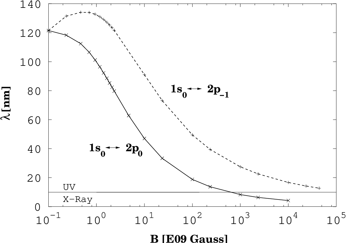
Finally, in Fig. (5) we show the wavelengths $\lambda={2\pi}/{\alpha\,(E^{\tau^{\prime}}_{b}-E^{\tau}_{b})}$ ($\alpha\simeq 1/137$ is the fine structure constant and $(E^{\tau^{\prime}}_{b}-E^{\tau}_{b})$ is the (variational) energy difference between the initial and final states) of the electromagnetic radiation associated with each transition as function of the magnetic field strength $B$. From Fig. (5), we can see that the wavelength of the longitudinal polarized radiation in the transition $1s_{0}\leftrightarrow 2p_{0}$ is a monotonously decreasing function of the magnetic field, reaching the domain of X-rays for $B\sim 10^{12}$ G, while the wavelength of the right polarized radiation corresponding to the transition $1s_{0}\leftrightarrow 2p_{-1}$ increases for small to weak magnetic fields reaching a maximum⁴⁴ 4 Hydrogen transitions whose wavelengths go through maxima or minima as functions of the magnetic field are called stationary lines. for $B\sim 0.2$ a.u. (with $\lambda_{max}\sim 1340.7$ Å), and decreasing for larger magnetic fields. Yet, this transition remains always visible in the UV-region even for the stronger magnetic fields considered in the present study $B\sim 10000$ a.u.

Figures (2), (3) and (4) show the results of the calculations for the dipole strengths, oscillator strengths and transition probabilities (formulas (5), (6) and (7) respectively) for the transitions $1s_{0}\leftrightarrow 2p_{-1}$, and $1s_{0}\leftrightarrow 2p_{0}$ in the domain of magnetic fields $B\sim 0.1-10000$ a.u. Tables (4) and (5) also show the results of those quantities for magnetic fields $B=0-10000$ a.u.