The Effect of Large-Scale Power on Simulated Spectra of the Ly forest
Abstract
We explore the effects of size of the box that we use for simulations of the intergalactic medium (IGM) at redshift two. We examine six simulations from the hydrodynamic code ENZO using the same cosmological and astrophysical input parameters and cell size, but different box size. We study the CDM distribution and many statistics of the Ly forest absorption from the IGM. Larger boxes have fewer pixels with significant absorption (flux ), more pixels in longer stretches with little or no absorption, and they have wider Ly lines. The larger boxes differ only because they include power from long wavelength modes that do not fit inside the periodic conditions of the smaller boxes. The long modes change the density, velocity and temperature fields and these increase in the gas temperature. Small simulations are too cold compared to larger ones. When we deliberately increase the heat we put into the IGM, we can approximate the Ly forest in a simulation of twice the size. When we double the box size, the difference of most statistics from their value in our largest 76.8 Mpc box is reduced by approximately a factor of two. Most of the statistics converge towards their value in the simulation with the largest box size, though line widths are not yet converged and the most common value of the CDM density shows no sign of converging, because the larger boxes include places with ever higher densities. These regions are not in the IGM, but they may produce the strongest of Ly lines.
When we double the box size from 38.4 Mpc to 76.8 Mpc, the mean Ly absorption decreases 0.5%, the frequency with which we encounter different common CDM densities changes by 2%, typical Ly line widths, the frequency of flux values and the power spectrum of the flux all change by 4–7%, and the column density distribution changes by up to 15%. When we compare to the errors in data, we find that our 76.8 Mpc box is larger than we need for the mean flux, barely large enough for the column density distribution and the power spectrum of the flux, and too small for the line widths that increase by 1 km s-1 when we increase the box from 38.4 Mpc to 76.8 Mpc, which is approximately the error in data. We can most readily see the effects of the long wavelength modes in measurement on the smallest scales in the Ly forest, the line widths, because they are easier to measure than the long wavelength power. Our optically thin simulations have a factor of several too few lines with H I column densities cm-2. Reducing the cell size from 75 to 18.75 kpc is not a solution. Our simulated spectra have 20% less power than data on small scales and 50% less on large scales, and their Ly lines are 2.6 km s-1 too wide. We do not see how our simulations might match all data at . Reducing the cell size to 18.75 kpc lowers the Ly line widths by 1.8 km s-1, but radiative transfer effects can increase them by as much as 1.3 km s-1 at z=2.5. We might reduce line widths using a softer ionizing spectrum to reduce heating, or we could use that has the additional benefit of increasing the large scale power. It is hard to see how simulations using popular cosmological and astrophysical parameters can match the Ly forest data at .
Keywords:
quasars: absorption lines – cosmology: observations – intergalactic medium – numerical simulations.1 Introduction
We are exploring the physical conditions in the IGM and the history stored in those conditions. We retrieve the physical conditions by finding numerical simulations that give simulated spectra that have H I Ly forest absorption that are statistically similar to real spectra. Data on the IGM can give relative errors of the order of a few percent for statistical properties of the forest. In Jena et al. 2005 (J05) we showed that at redshift 1.95 our simulations using typical cosmological and astrophysical parameters gave a good match to both the mean flux transmitted in the Ly forest and the -value distribution that we use to describes the Ly line widths. We noted that the power spectrum of the flux for these simulations was broadly similar to that of data. However, we spent little time with the power, and we did not attempt to run any simulations that gave exactly the mean flux and -values of data.
Here we explore one aspect of the accuracy of our simulations, the dependence on size of the simulation box. We discuss various statistics, including the mean flux, the flux probability distribution function (pdf), the typical -value, the pdf of the -values, the power and autocorrelation of the flux and the density and power of the CDM. We restrict our attention to one cosmological model at one epoch, and we say little or nothing about other relevant factors such as redshift evolution, the tilt of the initial power spectrum of fluctuations and a measure of the amplitude of the density fluctuations today, . We also do not discuss other important aspects of the simulations, including the accuracy of the initial conditions, the redshift where the simulations begin (Heitmann et al. 2006; Lukic et al. 2007) the accuracy of the potential and hydrodynamical evolution (Regan et al. 2007), the ionization and heating and the lack of radiative transfer. In J50 we showed how cosmological and astrophysical parameters, and the box and cell size change the mean flux and -values. Here we cover many more statistics of the Ly forest in a more quantitative manner.
It is now well known (Kauffmann & Melott 1992; Pen 1997; Barkana & Loeb 2004; Sirko 2007), that we need box sizes of many hundreds of Mpc to measure the power of the matter accurately. For CDM (gravity) alone we can now run simulations that are large enough to capture most of the variations from large scale modes (Neto et al. 2007). However, we can not yet run large enough hydrodynamic simulations with the kpc cell size required (Meiksin & White 2004) in the IGM, although we could instead run an ensemble of simulations, each with a different mean density (Mandelbaum et al. 2003). Meiksin & White 2004, for example, study the convergence properties of the flux power spectrum and autocorrelation function and recommend a box size of 25 Mpc but only for high redshifts () and even then they do not find convergence to better than 10%. Similarly, (Bagla & Ray 2005) study the effects of box size on halo mass functions and indicate that a minimum box size of several 100 Mpc is needed.
A secondary goal of this work is to make it easier to obtain validated and reproducible results on the Ly forest, in accord with the sentiments of the “Cosmic Code Comparison Project” (Heitmann et al. 2007). Hence we deliberately include many tables and figures to aid comparisons with other simulations.
In §2 below, we briefly describe the simulation code and parameters we have adopted. In §3 we describe the statistics of the cold dark matter distribution. §4 describes the statistics of the flux in the Ly forest including the mean flux, flux distribution, and line -values and column densities. In §5 we give the power of the flux spectra and the autocorrelation. In §6 we give the velocity field, baryon temperature and density. In §7 we show how putting more heat into a simulation makes its Ly forest appear like a simulation of twice the box length. In §8 we discuss an ambiguity present in the way flux power is calculated. In §9 we discuss how cell size, or resolution changes the Ly forest statistics. In §10 we show how the different statistics converge on the values in large boxes and we compare to data. In §11 we review the physical causes of the changes we saw with box size. The appendices contain technical details: A how we make spectra, B how we evolve them, C how we make extended sight lines, and D the lack of realistic variations in the density field.
Overall, the comparison with data shows some large differences that make it hard to see how simulations will be able to exactly match the current Ly forest data at using the popular cosmological and astrophysical parameters.
2 ENZO IGM Simulations
The numerical simulations (Bodenheimer et al. 2007) that we describe in this paper use the Eulerian hydrodynamic cosmological code ENZO (Bryan et al. 1995; Bryan & Norman 1997; Norman & Bryan 1999; O’Shea et al. 2004; O’Shea et al. 2005; Regan et al. 2007; Norman et al. 2007). The simulations contain both CDM and baryons in the form of gas, but no stars. The simulations were all run with the same cosmological parameters: a flat geometry = 1, comprising a vacuum energy density of , (CDM plus baryons), a baryon density of , a Hubble constant of = 71 km s-1 Mpc-1 and an initial power spectrum scalar slope of with a current amplitude of .
The ENZO code follows the evolution of the gas using non-equilibrium chemistry and cooling for hydrogen and helium ions (Abel et al. 1997; Anninos et al. 1997). After reionization at , photoionization is provided using the Haardt & Madau 2001 volume average UV background (UVB) from an evolving population of galaxies and QSOs. This gives photoionizations per second per H I atom at and photoionizations per second at . The simulations are optically thin so that all cells experience the same UV intensity at a given time. We do not treat the transfer of radiation inside the volume, and we include no feedback from individual stars or QSOs except for that implied by the uniform UVB.
As in J05, we use two parameters to describe the intensity of the UVB. The parameter is the rate of ionization per H I atom in units of the Haardt & Madau model discussed above, while measures the heat input per He II ionization, again in units of the rate for the Haardt & Madau spectrum.
We initiate the simulations using an Eisenstein & Hu 1999 power spectrum for the dark matter perturbations, that we insert at . The simulated volumes are all cubes with strictly periodic boundary conditions. Hence the power is input at a finite number of discrete wavenumbers. When we increase the box size, we insert the new modes that now fit inside the box, but we do not change the amplitudes of the smaller modes.
The amplitude of the power that we insert varies smoothly with wavenumber. We insert the amplitude expected for the universe as a whole, with no random variations associated with the finite box sizes. Since all our simulations use the same cosmological parameters, they all have exactly the same initial power for all modes that fit inside their box. The power in the simulations is not adjusted to include the variations in mean density that we see in the universe on the scale of the boxes. Hence, all the simulations are more similar to the mean of the universe than would be any observational measurement. We discuss this more in Appendix D. In this limited sense, the boxes contain information on scales much larger than their sizes.
We initiated all simulations using the same random number seed to generate the phases of all the modes. The phases are assigned to modes according to the mode direction and size measured in units of the box size (and not Mpc). Hence, in box units, the simulations have the same distribution of matter on the largest scales, as we show below.
We ran the simulations to , and all the results that we give refer to , except for specific cases discussed in Appendix B.
2.1 Series of Simulations
We will discuss three series of simulations with parameters listed in Table 1. The main A series have identical input parameters except for the box size. The larger boxes contain more total volume and mass and they contain power on scales that does not fit in the smaller boxes.
The A and KP series simulations have identical cosmological parameters and exactly the same comoving cell size of 53.25 or 75 kpc comoving. Each simulation has one CDM particle for each cell initially, and each dark matter particle, in each simulation, has a mass of . All the simulations are fully constrained by the input parameters since we do not re-scale any of the simulations outputs, such as the densities, H I, or fluxes.
| Simulation | Box | Cell | |||
|---|---|---|---|---|---|
| or box | (cells) | size | size | ||
| name | (Mpc) | (kpc) | |||
| A | 1024 | 76.8 | 75 | 1.0 | 1.8 |
| A2 | 512 | 38.4 | 75 | 1.0 | 1.8 |
| A3 | 256 | 19.2 | 75 | 1.0 | 1.8 |
| A4 | 128 | 9.6 | 75 | 1.0 | 1.8 |
| A6 | 64 | 4.8 | 75 | 1.0 | 1.8 |
| A7 | 32 | 2.4 | 75 | 1.0 | 1.8 |
| A2kp | 512 | 38.4 | 75 | 0.9217 | 2.165 |
| A3kp | 256 | 19.2 | 75 | 0.836 | 2.579 |
| A4kp | 128 | 9.6 | 75 | 0.738 | 3.045 |
| B2 | 512 | 9.6 | 18.75 | 1.0 | 1.8 |
| B | 256 | 9.6 | 37.5 | 1.0 | 1.8 |
| A4 | 128 | 9.6 | 75 | 1.0 | 1.8 |
| B3 | 64 | 9.6 | 150 | 1.0 | 1.8 |
Each A and KP series simulation is a cube with side length kpc. The A series simulations differ in size by factors of two, from the largest simulation A with cells to the smallest A7 with . The A simulation has comoving box side length of 54.528h-1 or 76.8 Mpc , while the A7 has sides of 1.704h-1 or 2.4 Mpc. The box for simulation A is 32 times larger in each dimension than A7, giving it a volume times larger. We also ran a simulation with cells but found it significantly different and of no value to us.
We discussed simulations A, A2, A3 and A4 in J05 for other purposes. We do not use the label A5 because this was a version of A4 described by J05. In J05 we noted a problem with A2. We have now re-run this simulation and we found that the problem was incorrect joining of the sub-grids of A2 presented in J05. The results presented for A2 in J05 were incorrect for the power spectrum, but correct for the flux and -values.
In the next few sections we discuss the A series simulations alone. We discuss the three simulations, A2kp, A3kp and A4kp, the KP series, in §7. They explore the effect of changing the heat input per He II ionization. We discuss the 4 simulations in the B series, which include A4, in §9 when we discuss changing the resolution of the simulations by changing the cell size.
3 The CDM Density Distribution
We discuss how the CDM density distribution varies with box size in the A series of simulations at . We do not discuss the baryons until §4.
In Figure 1 we show the frequency distribution of the CDM in the cells. We define the normalized-density of CDM as
| (1) |
where the denominator is the mean density of CDM in the universe at which is also the mean density of the CDM in all our simulations. The shape of the curve is expected from semi-analytical work (Lacey & Cole 1994) on the formation of dark matter halos.
The distributions of the densities for all simulations continue towards much lower densities than we show. The distributions become steeper with decreasing density, but otherwise we see no conspicuous features. Since the simulations initially have an average of one CDM particle per cell, most cells with contain no particles. Their densities can be non-zero because density is defined by distributing mass with immediately neighboring cells whenever a particle is not exactly centered in its cell. Hence a particle at the corner of a cube would contribute = 0.125 to each of the eight cells.
In Table 2 we list the percentage of the cells with zero density. This is 13.78% in simulation A, increasing systematically to 14.72% in A7. These cells have no immediate neighbors containing a CDM particle and we assigned them a nominal density of particles per cell, which we can ignore. We also list the minimum and maximum density in any cell.
The lowest density portions of the distribution are not physically realistic because we have too few particles per cell to accurately simulate densities far below the mean. We are more interested in the gravitational potential than in the density in a cell, and the potential is much smoother than the density distribution. The dark matter is smoothed twice, once when CDM is assigned to cells using the piecewise linear cloud-in-cell algorithm (Hockney & Eastwood 1988) and again when the potential is calculated. Where we have low dark matter densities, we may have low-level fluctuations in the potential due to particle discreteness. At worst, the CDM particles become mildly collisional.

The simulations in larger boxes contain higher densities, and hence they extend further to the right in Fig. 1. However, on the scale of this plot, all the simulations contain approximately the same frequencies at each density, with no variation with box size, which suggests that we will see little effect of box size on the statistics of the flux beyond those coming from the larger volumes and higher maximum densities in larger boxes. We do, however, see one minor difference between the boxes. Several simulations have frequencies lower by about a factor of two for the densities within a factor of a few of the largest value found in that simulation. This is conspicuous for A7 (red), A6 (orange) and A3 (blue), but not for A4 (green) and A2 (violet) which seem to follow A (black).
It is striking that we see almost no change with box size in the probability distribution function (pdf) of the CDM density per cell for the overdensities responsible for the Ly forest absorption, approximately 0.5 16. We obtain the typical baryon density corresponding to a given log NHI from Schaye 2001 who developed an analytic model that gives an excellent fit to simulations. Using the cosmology for the A series (= 0.27, = 0.044, H=71 km/s/Mpc) and the temperature-density relation from simulation A2 (, J05 Table 9) we find at
| (2) |
Lines in the Ly forest with log NHI= 12.5 – 14.5 cm-2 then come typically from baryon overdensities of 0.5 – 15.7. A larger range of densities is involved in making significant absorption in the Ly forest (Schaye et al. 2003). For this discussion we assume that the baryon and CDM density fluctuations are similar in amplitude. Gnedin et al. 2003 show that the baryon fluctuations are similar to the CDM fluctuations on scales larger than the filtering scale, with , where the filtering scale depends on the integral over time of the Jeans length and is approximately 0.055 s/km (11 Mpc-1) at (their Fig. 2).
| Name | Zeros | Min | NonL | Max | |
|---|---|---|---|---|---|
| (cells) | (%) | (%) | |||
| A | 1024 | 13.78 | 3.6810-11 | 4.67 | 1.64104 |
| A2 | 512 | 14.07 | 2.3210-10 | 4.68 | 1.41104 |
| A3 | 256 | 14.37 | 4.8610-9 | 4.71 | 5.71103 |
| A4 | 128 | 14.44 | 3.9210-8 | 4.79 | 3.12103 |
| A6 | 64 | 14.67 | 3.5010-8 | 4.85 | 8.25102 |
| A7 | 32 | 14.72 | 2.0910-7 | 4.91 | 3.01102 |
The statistics on the distribution of the density of CDM in Table 2 show that both the maximum and minimum density of CDM in any cell increases systematically with the box size. The minimum is not relevant to us; since we work with the density and not the log(density), these values are all essentially zero, but the maxima are important for the flux spectra.
In Figure 2 we zoom in on the densities that are more important for the flux in the Ly forest, and we expand the sensitivity by dividing by the frequencies found in simulation A. We now see systematic trends with box size. The larger boxes have higher frequencies of small densities, approximately log() , and lower frequencies of higher densities. All boxes have approximately the same frequency for log() , near the most common density. At densities below the most common, the largest difference from the A simulation is seen at lower densities in the smaller boxes. Above the most common densities, the largest differences from A are seen at near the mean density. The larger the box, the less the deviation from A. We anticipate that these differences will manifest as changes in the baryon density and hence the Ly forest.
In Table 3 we list two further statistics showing the changes in the CDM density per cell with box size, the RMS and the mean of the absolute difference (MAD), each relative to the value in to box A and averaged over . Both statistics decrease by about a factor of two for each doubling in box size, reaching an RMS of only 0.7% for simulation A2. We will see a similar rate of convergence for other statistics of the Ly forest (McDonald & Miralda-Escudé 2001).

| Name | MAD | RMS |
|---|---|---|
| (%) | (%) | |
| A | 0.00 | 0.00 |
| A2 | 0.57 | 0.70 |
| A3 | 1.23 | 1.44 |
| A4 | 3.01 | 3.32 |
| A6 | 7.11 | 8.23 |
| A7 | 14.30 | 17.79 |
3.1 Distribution of the variance of the density of CDM amongst sight lines
We will be examining the power of the CDM in the next section because this helps us understand how the simulations in general and particularly the power of the flux change with box size. Here we look first at the variance of the CDM because this is related to the sum of the power over all modes.
In Figure 3 we show the faces of the series A simulations. For each position in the plane, we show
| (3) |
the mean value of along the cells parallel to the axis which goes into the page. We consider these rows as sight lines, which we label with the subscript “” to indicate a choice of both and . We show this quantity because is the contribution of that sight line to the variance of in the whole simulation box, since
| (4) |
where is the number of cells in the simulation box, and if and only if it is the mean of the values of all cells in the box, following the definition of in Eqn. 1.
The quantity tells us how much that sight line contributes to the mean power of all sight lines. The quantity is not the variance along each sight line, , since that is the mean of , where the is the mean along each sight line. These means differ from sight line to sight line, and can be very different from unity.
Figure 3 looks similar to the projection of the density, since the is largest where we encounter a cell with a high density. If we shrink the squares from the smaller simulations to give constant Mpc per mm on the page, then the density and size of structures looks approximately the same in all simulations, although they are not the same, for example because the smaller boxes are also smaller in the direction.

In Figure 4 we show the distribution of the and in Table 4 we give some statistics. We have one for each sight line parallel to the axis of each simulation box. Larger boxes have a lower frequency of sight lines with small , their most common (mode) is larger, they have a higher frequency of larger , and larger maximum . This is because the larger boxes have more sight lines, each of which is longer, and there are higher densities in the larger boxes.


| Name | Min | Mode | Mean | Max |
|---|---|---|---|---|
| A | 0.61 | 3.55 | 175.78 | 1.14106 |
| A2 | 0.58 | 1.78 | 146.12 | 8.39105 |
| A3 | 0.50 | 0.71 | 122.84 | 2.49105 |
| A4 | 0.43 | 0.71 | 100.66 | 1.11105 |
| A6 | 0.36 | 0.71 | 53.38 | 2.24104 |
| A7 | 0.29 | 0.71 | 26.61 | 3.42103 |
The small boxes lack the high density peaks of the larger boxes because they lack volume, and they lack long modes. They do not contain enough particles to produce the highest densities. To make a peak with particles in a cell, we must collect particles from cells, more than are contained in the A7 simulation.
Bagla & Ray 2005 have explored how the frequency of high density CDM collapsed structures changes with effective box size. They use simulations with CDM particles in Mpc boxes with a softening length of Mpc. They find that the number of high density peaks decreases when they truncate the initial power spectra at lengths less than the full box size. They see a factor of three fewer collapsed structures with mass when they truncate the power at 1/4 of the box size. However, when they truncate at 1/2 the box size they see only an 80% reduction in the number, showing convergence to the result expected for a much larger box. This convergence happens for boxes 3 – 6 times larger than A.
3.2 Power of Normalized CDM Density
We compute the Fourier transform of , the normalized-density of CDM minus one,
| (5) | |||
| (6) |
where is the wavenumber, is the pixel index, is velocity and is the velocity width of a pixel with redshift width . Subtracting one has no effect on except for the mode with zero frequency. We take the transform of the density along each sight line parallel to and extending the full length of the axis. We did not explore the and directions. We use a discrete Fast Fourier Transformation algorithm, and we use
| (7) |
as our estimate for the one-dimensional power, where the brackets refer to averaging over all sight lines parallel to the axis.
Since the density distributions in the box is always strictly periodic, the power spectrum (of the signal along sight lines parallel to the axis) is non-zero for the discrete set of modes , where s=1,2,3… , and is the length of each spectrum in velocity units, corresponding to comoving Mpc. At redshift , km s-1Mpc-1, and simulation A has km s-1.
In Figure 5 we show the power spectrum of for the A series boxes. We begin each spectrum at the left at its fundamental mode, the smallest wavenumber for that box. For simulation A s/km. We end the plots on the right at the Nyquist frequency, s/km, or log s/km, where is the velocity width of a simulation cell, 5.027 km s-1 at .

The power is larger at all in the larger boxes, which we expect because the variance like quantity in Fig. 4 is also larger. The increase in power with box size is most pronounced on the largest scales. The power is larger in larger boxes even on the smallest scales. We now present a figure that shows that the increase in the power with box size is intrinsic to the density distribution, and not an artifact of the length of the sight lines or the number of sight lines through the boxes.
In Figure 6 we show power spectra obtained from simulation A6 using a reduced number of shorter sight lines. We divide the A6 cube into the eight sub-cubes, each of size A7, that together exactly fill A6. We made spectra from all the sight lines restricted to each sub-cube, and we took the power spectrum of each. We then distribute these power spectra randomly into the eight means, each of which contains some sight lines for each of the eight sub-cubes, and the same total number of sight lines as does the mean power spectrum of A7. We see that the power in the sub-cubes is distributed about that in A6, and not A7. This shows that the extra power in A6 is intrinsic to the density distribution in A6, and not from the length or number of sight lines. The dispersion of the power in the 8 spectra gives one indication of the random error in the power of the A7 simulation.

3.3 Power from Density Peaks
Parseval’s Theorem states that sum of the power at all modes is proportional to the sum of the square of the signal. Using the signal from Eqn. 4, we have
| (8) |
where is the number of cells in a box, and P(k) has velocity units that cancel the inverse velocity units on the . This can also be written as
| (9) |
which shows that the mean value of averaged over all cells in the box, is equal to the sum of all modes in the power (which is also averaged over all sight lines), divided by the length of each spectrum. This is the normalization used by McDonald et al. 2006 (Eqn. 12). It is the “System 2” normalization from Bracewell 1986 (p. 7).
The values show how the sum of the power at all modes is distributed amongst the sight lines. We saw in Fig. 4 and Table 4 that a few sight lines have values vastly larger than the mean. This means that these few sight lines also dominate the total power of each simulation.
In Figure 7 we show a single 1024 pixel line of sight from simulation A with a density peak of . This peak increases the power about 1000 times over a wide range of wavenumbers. The density spike is narrow in velocity space, and hence wide in space (e.g. Fig. 6.2 of Bracewell 1986). In the lower right panel we see that smoothing the density spike removes most of the excess power.


We can estimate the amount of power added quantitatively. A typical sight line from simulation A has of order 3 (Table 4). One pixel with a normalized-density of 1700 increases the variance to , approximately the increase we see in the integrated power. Hence, a single sight line with a normalized-density will contain as much power as the whole cube of sight lines each with typical variance. Simulation A contains 77 cells with and 12 with , sufficient that these few cells, and the sight lines that pass through them, will dominate the power spectrum of the (un-smoothed) CDM.
In Figure 8 we show how the sum of the of the sight lines increase with the number of sight lines included. We start on the left with the sight lines with the smallest , ending on the right with those with the largest. We see that, for all simulations, the few sight lines with the largest completely dominate the total. Depending on the simulation, 90% of the total comes from only 2 to 10% of the sight lines. The total , and hence the total power, is an unstable quantity, which can change significantly as the few highest density peaks changes in number and density.

We have shown that the power of the CDM density is larger in larger boxes primarily because larger boxes contain rare regions with higher density. We also see higher power because we use longer sight lines in the larger boxes. As Bagla & Ray 2005 showed, there is some effect from having longer modes in the larger boxes. However, Figs. 1, 2 showed only small changes in the frequencies of different densities per cell, which suggest that the extra long modes have a small effect on the quantities that we are evaluating.
When we examine the flux transmitted through the IGM we are most interested in densities near the mean. Although the larger boxes have higher maximum densities, they have slightly lower portions of their volume above a moderate density. In Table 2 the column NonL gives the fraction of cells with CDM density exceeding 3 times the mean. This fraction decreases systematically with box size, from 4.91% for A7 to 4.67% for A.
4 Statistics of the Flux in the Ly Forest
We make flux spectra using code described in Zhang et al. 1997 and J05. We make each spectrum along a row of cells parallel to the axis of the boxes, just as we did for the values that describe the variance of in §3.1. We use a number of pixels equal to the box side length .
In Figure 9 we show spectra of the flux along some random, unrelated sight lines through the A series simulations. We show equal total velocity length for all simulations, and hence for A7 we show 32 disjoint spectra, each separated by a vertical dotted line. We should ignore the vertical discontinuities where spectra end inside an absorption line. These tend to make lines look narrower, especially in the smaller boxes where there are more discontinuities. We see two major trends with box size.
The larger boxes contain large velocity intervals with very little absorption. These stretch over many hundreds of km/s, longer than the size of the smaller boxes. The larger the box, the longer the regions with little absorption. These low absorption regions are clearly showing correlation in the density on large scales. We would not expect to see them as often if we truncated the power to include only short modes.
The smaller boxes seem to have more absorption in total. The values that we list in the figure caption show this is correct for the A6 and A7, but the larger simulations have nearly identical mean flux. The smaller simulations also have a higher proportion of pixels with flux within a few percent of the continuum, and they have fewer lines of depth 5 – 50%. The number of the deepest lines seems approximately constant.

4.1 Statistics of Flux Spectra
In Table 5 we list statistics of the flux for the spectra from the simulations. The statistics are from each pixel in all spectra through each box in the direction. The values are the mean flux that we should add onto the current value to obtain that in the next larger box. The overall trend of the mean flux with box size is hard to discern because the changes are small compared to the measurement errors (discussed below). The underlying trend is apparently for larger mean flux in larger boxes, but this seems to reverse for the largest 4 boxes, where the flux decreases in the larger boxes.
| Name | error | Mode() | |||
|---|---|---|---|---|---|
| A | 0.8714 | 0.0039 | ….. | 0.051 | 0.8875 |
| A2 | 0.8721 | 0.0059 | -0.0007 | 0.058 | 0.9075 |
| A3 | 0.8734 | 0.0113 | -0.0013 | 0.060 | 0.9325 |
| A4 | 0.8741 | 0.0168 | -0.0007 | 0.067 | 0.9375 |
| A6 | 0.8612 | 0.0332 | 0.0129 | 0.073 | 0.9575 |
| A7 | 0.8335 | 0.0531 | 0.0277 | 0.095 | 0.9725 |
| A2kp | 0.8716 | 0.0059 | -0.0002 | 0.058 | 0.9075 |
| A3kp | 0.8707 | 0.0118 | 0.0009 | 0.058 | 0.9275 |
| A4kp | 0.8701 | 0.0181 | 0.0006 | 0.063 | 0.9325 |
We estimated the errors on the mean flux values in Table 5 from the standard deviation of the mean flux values for tiles across the face of each box. We use tiles of continuous area because the spectra in adjacent sight lines are highly correlated, and hence the error on the mean flux value is much larger than the standard deviation divided by the square root of the number of samples. We use a 4x4 tiling for A and A2, 3x3 for A3 and A4 and 2x2 for A6 and A7. These choices are a compromise between having enough tiles to give a small random error and having tiles large enough to reduce the inter-tile correlations.
The error given by tiling captures some of the variation in the mean density on large scales across the boxes. However it is less than the external error that we would want to use when we compare to real spectra because it misses all of the variation that we would see if we started each box with different random phases, and we allowed each mode to have a random amplitude, and it misses the variation due to all modes larger than the box. On the other hand, this error from tiling is larger than the smallest change that we can consider indicative of a trend when we compare a series of boxes. This is because the statistics are evaluated from the whole of each box and all boxes use the same amplitudes and phases for their modes.
In Table 5 we also list the variance of the flux evaluated for all sight lines through the box, where is the mean flux in the box, and not that in each sight line. We have , where the sum is over all pixels from all spectra though one side of the box. The variance of the flux in each pixel is then . The quantity decreases systematically with increasing box size, because, we will now see, the fraction of pixels with flux is up to a factor of two smaller in the larger boxes.
In Figure 10 we show the distribution of the flux per pixel for all spectra through each A series simulation, also called the flux pdf. In Figure 11 we show the same value, divided by the fractions for simulation A. The simulations all have approximately the same frequency of pixels with a flux of 0.96 – 0.97. The larger simulations have higher frequencies above 0.97, and lower below. Our impression that the spectra from the smallest boxes have more absorption is confirmed; they do have a much larger fraction of pixels with . We also confirm that the larger simulations have more pixels with very high flux. We see smaller changes between the larger simulations, indicating convergence by the size of box A. If this trend continues, then the fractions for simulation A will be within approximately 5% of those for a much larger simulation.


We see that the differences between the simulations decrease to less than 10% for fluxes below 0.02; they all have the same fraction of their spectra occupied by the bottoms of saturated absorption lines. This is reasonable because Figs. 1 and 2 show they all have approximately the same frequency (per Mpc3) of high density regions. The largest differences between the boxes are for intermediate flux levels from the sides of saturated lines, or the bottoms of nearly saturated lines, both of which are a small fraction of the pixels.
In Table 5 we also list Mode() the mode of the mean flux values, , with one mean per sight line. The modes are the most common mean fluxes when we use bins of 0.0005. In contrast with the mean flux per pixel, these modes per sight line show a systematic decrease with increasing box size. These modes are all much less than the mode of the flux in individual pixels, which is 0.990 to 0.995 for all boxes, as seen in Fig. 10.
4.2 Statistics of the Lines
In this section we quantify the types of lines seen in the simulations. We obtain line statistics by fitting Voigt profiles as described in Zhang et al. 1997. As in Tytler et al. 2004 and J05 (§5.1, 6.2) we consider only lines with cm-2. We also limit our discussion to lines with central optical depths , which is a new constraint for this paper.
4.2.1 Line Widths: -values
In Figure 12 we show the distribution of the -values. The distributions show small but clearly systematic changes with box size. In detail, the larger boxes have wider lines, fewer narrow lines with km s-1, and more lines with km s-1, and a slightly broader distribution. The smallest box A7 is an exception to this, presumably because the fundamental mode in this box is nonlinear at . The change in typical line width can come from a combination of three factors: larger absorbing regions, giving more Hubble flow across a line; larger peculiar velocities from the increase in large scale power; and higher temperatures also from the increase in velocities (Theuns et al. 1999; Bryan et al. 1999).

In Fig. 13 we see that the -value distribution is sensitive to the minimum line central optical depth . We use a sample with log NHI cm-2 and . If instead we use a sample with we see a different value distribution that has a larger fraction of lines with km s-1 and a smaller fraction of lines with larger -values. Our sample is the subset of the total which lacks broad shallow lines. The shape of the distribution in the figure comes from the simultaneous requirement that log NHI (cm-2) and . Narrow lines with log NHI always have and hence they are not effected by the 0.05 limit. Very broad lines often have log NHI and .

In Tytler et al. 2004 we showed that Hui & Rutledge 1999 function gave an excellent fit to the distribution of -values from a simulation B, which had 35 kpc cell size, half of that used here. The Hui-Rutledge function has only one parameter, the that describes the typical line width.
In Table 6 we give estimates for the values that best fit the distributions of the lines from each simulation. We use the maximum likelihood method since it treats the individual -values, and not the binned values that we show in the plots. We make two improvement on J05. First, we now fit only lines with km s-1 because we want to describe the most common lines, and not the rare broad features that are hard to see in real spectra because of photon noise, flux calibration problems and uncertain continua. When we included all -values in J05 the was larger by about 0.5 km s-1. Second, we completely sample the boxes, where as J05 had few spectra, all of which began at the lowest density part of that box. The values that we give here differ from those that we gave in J05 for the same simulations for these reasons. We estimate the errors using the tiles, as we did for the for the mean flux, and again the same comment apply; external errors are larger, and we can be interested in differences between boxes that are less than the external errors. We did not estimate the errors for B, B2 and B3 but we give the value of 0.8 km s-1 from A4 because these boxes are all the same size and contain the same number of Ly lines of a given NHI.
| Name | error | ||
|---|---|---|---|
| (km s-1) | (km s-1) | (km s-1) | |
| A | 26.7 | 0.2 | … |
| A2 | 25.6 | 0.4 | 1.1 |
| A3 | 24.8 | 0.5 | 0.8 |
| A4 | 24.1 | 0.8 | 0.7 |
| A6 | 22.4 | 1.2 | 1.7 |
| A7 | … | … | … |
| A2kp | 26.2 | 0.4 | 0.5 |
| A3kp | 26.3 | 0.5 | 0.1 |
| A4kp | 26.3 | 0.7 | 0.0 |
| B2 | 22.3 | 0.8 | … |
| B | 22.1 | 0.8 | 0.2 |
| A4 | 24.1 | 0.8 | 2.0 |
| B3 | 28.3 | 0.8 | 4.2 |
The mode of the -value distribution is . We do not list for A7 because this box is barely large enough to contain a single complete line, and we do not obtain fits to -values. The -values show a simple trend: a systematic increase with increasing box size, consistent with the change in shape of the pdf of the -values. We discuss the convergence behavior of this statistic in §10.
4.2.2 Column Density Distribution:
In Figure 14 we show the distribution of the H I column densities of the lines, relative to the values for box A. Here the function is the differential distribution of lines, per (linear) cm-2, and per unit absorption distance . The coordinate is defined such that the density of absorbers per unit should be independent of and . The number density of non-evolving objects per unit redshift along a line of sight is given by (Tytler 1981, Eqn. 3)
| (10) |
where and we define the function
Setting , can then be defined (Tytler 1982) using , which gives
| (11) | |||||
Until this decade it was common to use models with = 0 and or 1/2. We now use the cosmological parameters that we gave in §2, = 0.73 and = 0.27, which at give . For the value of is similar, but for we have the significantly different value . A single sight line through the A box then covers where and is the velocity span of one sight line, 5143.37 km s-1.
Larger boxes have larger maximum column densities. The smallest box A7 has no lines with log NHI cm-2 while the larger boxes have a higher density of lines with log NHI cm-2. Indeed the trends are rather complex with e.g., box A showing a noticeably higher density of systems with log NHI cm-2 than all the other boxes. We see strong correlations between the values for similar values because adjacent sight lines sample almost the same absorbing gas and hence almost the same column densities. We also see large deviations when NHI changes by about a factor of ten. Together these features make it hard to assess the errors and rate of convergence.
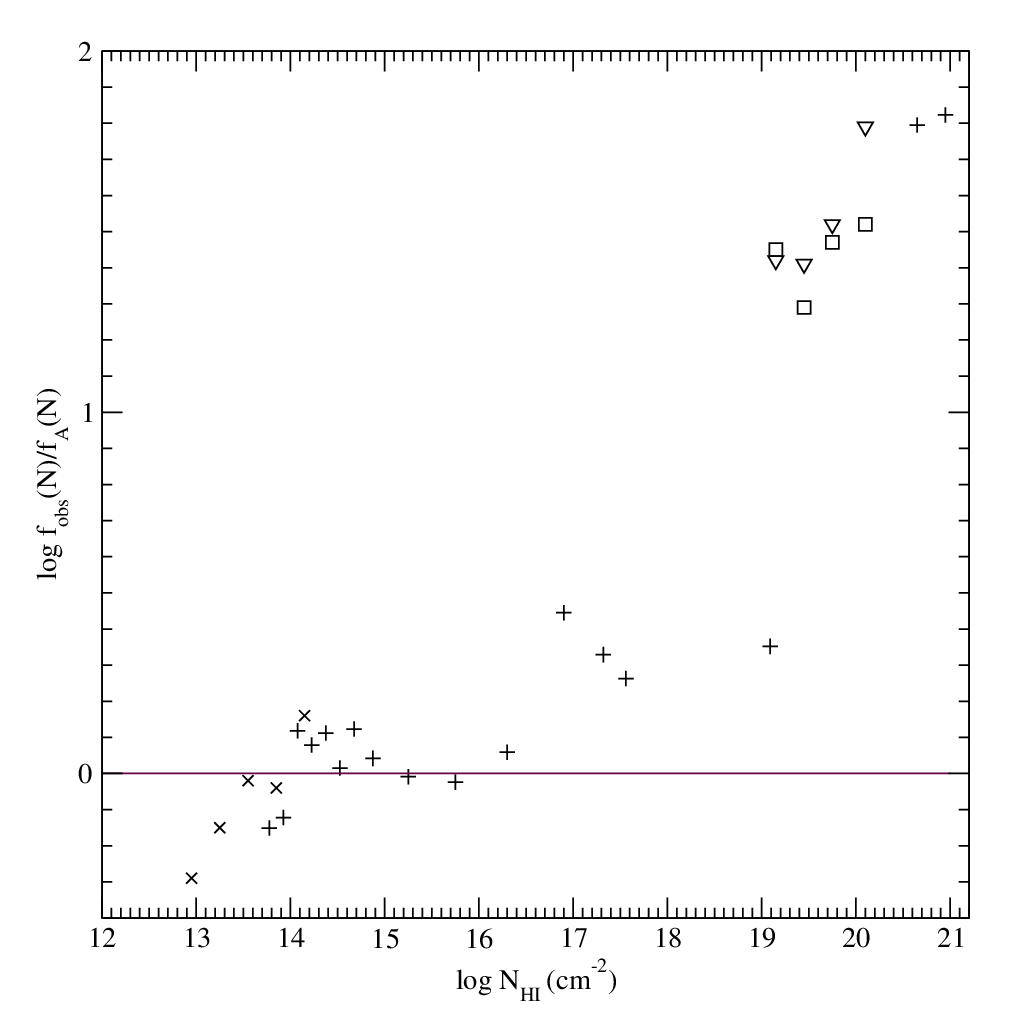
In Figure 15 we compare observed values for the column density distribution to the values from box A. We list values for box A in Table 7. We have attempted to correct the data to and our definition.
| log NHI | log NHI | ||
|---|---|---|---|
| (cm-2) | (cm2 X-1) | (cm-2) | (cm2 X-1) |
| 11.5 | 9.80489 | 16.3 | 16.9895 |
| 11.7 | 9.91356 | 16.5 | 17.2893 |
| 11.9 | 10.0239 | 16.7 | 17.5894 |
| 12.1 | 10.1645 | 16.9 | 17.9246 |
| 12.3 | 10.3565 | 17.1 | 18.2563 |
| 12.5 | 10.5504 | 17.3 | 18.5748 |
| 12.7 | 10.8223 | 17.5 | 18.9155 |
| 12.9 | 11.1150 | 17.7 | 19.1734 |
| 13.1 | 11.4108 | 17.9 | 19.4402 |
| 13.3 | 11.7170 | 18.1 | 19.7179 |
| 13.5 | 12.0511 | 18.3 | 20.0306 |
| 13.7 | 12.3695 | 18.5 | 20.3788 |
| 13.9 | 12.7416 | 18.7 | 20.7238 |
| 14.1 | 13.1143 | 18.9 | 21.1386 |
| 14.3 | 13.4898 | 19.1 | 21.5316 |
| 14.5 | 13.9236 | 19.3 | 21.8351 |
| 14.7 | 14.2540 | 19.5 | 22.1258 |
| 14.9 | 14.6523 | 19.7 | 22.4385 |
| 15.1 | 15.0434 | 19.9 | 22.7923 |
| 15.3 | 15.4000 | 20.1 | 23.1537 |
| 15.5 | 15.7948 | 20.3 | 23.5523 |
| 15.7 | 16.0774 | 20.5 | 24.0321 |
| 15.9 | 16.3919 | 20.7 | 24.3957 |
| 16.1 | 16.7003 | 20.9 | 24.8255 |
Numerical simulations have often found too few systems with high NHI values (Katz et al. 1996; Gnedin 1998; Gardner et al. 2001; D’Odorico et al. 2006). Simulations need both sufficient volume to contain the long wavelengths modes to get enough CDM halos (Bagla & Ray 2005), and they need high enough resolution to make the clumps of gas that cause Lyman limit systems (LLS). In recent work, Kohler & Gnedin 2007 are able to reproduce both the mean flux in the forest and the column density distribution of LLS at in Mpc boxes with kpc resolution. They also obtained approximately the real number of LLS per unit .
Our simulations lack absorption systems with large column densities. We lack a factor of 1.2 for log NHI cm-2. We see an increasing lack at log NHI cm-2, reaching a factor of approximately 30 by log NHI cm-2, and a factor of 70 for Damped Ly lines (DLAs) with log NHI cm-2. The point shown as a plus from Petitjean et al. 1993 is unreliable at log NHI cm-2. We are also uncertain about the errors in the measurements, especially since we have not checked that the values are consistent with the total mean absorption that we assume at . Our simulation A has approximately the correct total absorption, and hence the excess lines with log NHI cm-2 should make approximately the same total absorption as the lack with log NHI cm-2.
The lack at the higher columns, log NHI cm-2 is due to insufficient numerical resolution in collapsed halos which give rise to this absorption and the lack of self-shielding against the UV background radiation. The lack is large enough that we must clearly remove high column lines from both simulations and real spectra when we want to make quantitative comparisons, as first pointed out by Tytler et al. 2004 and Jena et al. 2005.

5 1D Power Spectra of the Flux
Following Croft & Gaztanaga 1997 and others, we define the flux contrast as
| (12) |
where is velocity and is the mean of the flux from all spectra through a box, listed in Table 5. While our signal looks like that used by Croft et al. 1998 and McDonald et al. 2000, there is an important difference. They both take to be the mean flux in each spectrum. We discuss this alternative choice below in §8.
Since the mode of the flux in each pixel is larger than the mean flux, is typically larger than zero. This definition resembles that of -1, except that involves division by the mean density of CDM that is a parameter input into the simulations and identical for all. In contrast, the mean flux is not known until spectra are made, and it varies from simulation to simulation and with .
We compute the Fourier transform of the flux contrast using in place of -1 in Eqn. 5. We measure the (one-dimensional) flux power of each sight line in the direction, and we present the average of the power from all sight lines. We have explicitly checked that we obtain the same power as does McDonald from the same spectrum.
In Figure 16 we show the power spectrum of the flux, , in this case from all spectra parallel to the axis in each simulation. We tabulate values in Tables 8 and 9, and in Figure 17 we show the power divided by that in simulation A. In contrast to the CDM power, the differences between simulations are small, and of the opposite sign. In general, the larger boxes have smaller flux power, the opposite of the trend that we saw in Fig. 5 for the power of the CDM. On the largest scale sampled by a box, the power at log s/km in the A2 and A3 boxes is slightly less than that in the largest A box. This might be simply the effect of the larger modes in the larger boxes. On intermediate scales there is a systematic decrease in power with increasing box size, with larger changes on smaller scales (larger ). However, on the smallest scales, log s/km, corresponding to sine wavelengths km s-1 (4 cells in the simulation), the trends change direction. The differences between the simulations become less, and A2 returns to approximately the same power as A. The largest deviations in the ratios of the power of the flux are seen at log (s/km), corresponding to changes in the shapes of the narrow lines.
| Box | log | log | log | log | ||||
|---|---|---|---|---|---|---|---|---|
| A | 0.933 | 0.757 | 0.239 | -1.310 | 1.00 | 1.00 | 1.00 | 1.00 |
| A2 | 0.910 | 0.739 | 0.246 | -1.279 | 0.95 | 0.96 | 1.02 | 1.08 |
| A3 | ….. | 0.767 | 0.253 | -1.233 | ….. | 1.02 | 1.03 | 1.20 |
| A4 | ….. | 0.742 | 0.325 | -1.144 | ….. | 0.97 | 1.22 | 1.47 |
| A6 | ….. | ….. | 0.336 | -1.060 | ….. | …. | 1.25 | 1.78 |
| A7 | ….. | ….. | ….. | -0.945 | ….. | …. | …. | 2.32 |
| A2KP | 0.919 | 0.747 | 0.244 | -1.325 | 0.97 | 0.98 | 1.01 | 0.97 |
| A3KP | ….. | 0.784 | 0.255 | -1.314 | …. | 1.07 | 1.04 | 0.99 |
| A4KP | ….. | 0.778 | 0.342 | -1.238 | …. | 1.05 | 1.27 | 1.18 |
| log | (km/s) | error | errore | |
|---|---|---|---|---|
| -2.9134 | 10.016 | 10.021 | 0.441 | 0.441 |
| -2.6124 | 9.371 | 9.377 | 0.409 | 0.411 |
| -2.4363 | 8.134 | 8.135 | 0.381 | 0.382 |
| -2.3114 | 7.576 | 7.576 | 0.363 | 0.364 |
| -2.2144 | 6.865 | 6.872 | 0.311 | 0.311 |
| -2.1353 | 6.446 | 6.447 | 0.283 | 0.284 |
| -2.0683 | 6.053 | 6.057 | 0.270 | 0.270 |
| -2.0103 | 5.790 | 5.794 | 0.250 | 0.251 |
| -1.9592 | 5.407 | 5.412 | 0.236 | 0.237 |
| -1.6830 | 3.264 | 3.260 | 0.124 | 0.123 |
| -1.5155 | 1.855 | 1.849 | 0.651(-1) | 0.648(-1) |
| -1.3949 | 1.068 | 1.068 | 0.315(-1) | 0.314(-1) |
| -1.3006 | 6.243(-1) | 6.256(-1) | 0.170(-1) | 0.171(-1) |
| -1.2232 | 3.748(-1) | 3.749(-1) | 0.106(-1) | 0.107(-1) |
| -1.1575 | 2.269(-1) | 2.273(-1) | 0.600(-2) | 0.620(-2) |
| -1.1005 | 1.376(-1) | 1.376(-1) | 0.375(-2) | 0.380(-2) |
| -1.0501 | 8.435(-2) | 8.398(-2) | 0.226(-2) | 0.229(-2) |
| -1.0049 | 5.185(-2) | 5.171(-2) | 0.149(-2) | 0.149(-2) |
| -0.8565 | 7.716(-3) | 7.725(-3) | 0.266(-3) | 0.272(-3) |
| -0.6630 | 2.878(-4) | 2.904(-4) | 0.137(-4) | 0.140(-4) |
| -0.5296 | 2.210(-5) | 2.215(-5) | 0.121(-5) | 0.127(-5) |
| -0.4277 | 3.272(-6) | 3.633(-6) | 0.196(-6) | 0.269(-6) |
| -0.3452 | 7.803(-7) | 9.018(-7) | 0.451(-7) | 0.954(-7) |
| -0.2759 | 2.357(-7) | 3.350(-7) | 1.341(-8) | 5.048(-8) |
| -0.2162 | 1.296(-7) | 2.193(-7) | 7.166(-9) | 3.727(-8) |
| -0.2041 | 1.286(-7) | 2.073(-7) | 7.110(-9) | 3.522(-8) |

The large changes in the power of the CDM with box size, contrasted with the small changes in the power of the flux implies that the bias will change rapidly with box size, approximately as does the CDM. Attention must be given to the appropriate smoothing of the fields to reduce the sensitivity of the CDM power to the box size (McDonald et al. 2002).
McDonald 2003 shows how the power of the flux changes when he increases his box size from 28.2 to 56.3 to 112.7 Mpc, while keeping the cell size constant at 220 kpc. He also sees that the power is lower in the smaller boxes
We see that the change in power with box-size is consistent with the simultaneous change in the -value distribution. Viel et al. 2003 showed quantitatively how power of the flux on small scales responds to changes in line -values. For log Viel et al. 2003 saw essentially the same power from randomly placed Ly lines as from real spectra. They also showed that making all -values larger by a factor of two decreased the power at log . Our larger boxes have larger -values and they show decreased power on these scales. If all other factors are unchanged, we would expect higher temperatures for the IGM in larger boxes, which we confirm in §6.2.

5.1 Autocorrelation of the Flux
Although containing exactly the same information as the power, the autocorrelation can better illustrate characteristics of the signal that are hard to see in the power, such as correlations over large scales. While a power spectrum is a complete statistical description of a random Gaussian field, the flux distribution is far from Gaussian, hence neither the power spectrum nor the autocorrelation will be a complete description.
The autocorrelation of the flux for a given velocity shift can be computed directly from a transmission spectrum as , where is the mean flux in a box from Table 5. The brackets refer to an average across the pixels of the spectrum. We choose to obtain the autocorrelation from
| (13) |
where is the power of the flux contrast and we can use the line of sight averaged power directly because we have divided by the mean flux of each cube. The results we report here, as with the flux power, are the average autocorrelation profiles at each velocity shift from all lines of sight.
For the power spectrum, the longest non-zero mode is one wave in the box. By analogy, for a sight line parallel to the box edges, the largest lag in a box is . We expect the autocorrelation to decrease up to scales of and then to rise again, since a lag of in one direction is simultaneously a lag of in the reverse direction. This is in contrast with real spectra where the autocorrelation will continue to decrease with increasing lag. The number of samples of each lag drops from for lags of one pixel to N/2 for lags of L/2. When we shift a spectrum by some lag, we loop around the periodic boundary conditions, making the first and last pixels adjacent, so that all shifted spectra have the same length.
In Figure 18 we show the autocorrelation of the flux calculated using the mean of the flux from all spectra through each box. The autocorrelation of the flux falls with increasing lags, and it falls to lower values in larger boxes. The larger boxes also have smaller correlation for most velocity lags. However, the autocorrelation does not drop to zero on the largest scales in a box, rather it stops falling at some low plateau value.


If we define the autocorrelation using the mean flux in each sight line , instead of the mean of the box, then the autocorrelations are all reduced. We show these autocorrelation functions as dashed lines in Fig. 18. The amount by which the two autocorrelation calculations differ is equal to the variance of the line of sight mean flux values about their mean, which is the mean flux of each cube that we give in Table 5,
| (14) |
where is the number of sight lines we use to sample each box. The smaller boxes have larger sight-line to sight-line variance, as can be seen in Fig. 19 and hence their autocorrelation (and other statistics) is decreased the most then we use the mean flux per sight line.
6 Velocity Field, Baryon Temperature and Baryon Density
Having seen how the statistical properties of the Ly forest depend on box size we now return to the examine the changes in the velocity field, and the baryon temperature and baryon density in the simulations, since these fields control how the Ly forest changes.
6.1 How gas velocity changes with box size
In Fig. 20 we see that the velocity of the cells increases dramatically with increasing box size. Velocities km s-1 are common in the three largest boxes but non-existent in the two smallest boxes. In Table 10 we list the minimum, median and maximum baryon velocity in each box. These velocities increase by factors of 1.23 – 2.59 as we double the box size, with the largest factors applying to the maximum velocity for the smallest pair of boxes. The maximum changes the most because this is sensitive to the rare high density regions. However, all cells show a systematic increase in velocity, as illustrated by the factor of 1.34 increase in the median velocity going from the A2 to A box.

| Box | mean | median | max |
|---|---|---|---|
| A | 136.4 | 138.2 | 1153.9 |
| A2 | 110.8 | 103.0 | 764.3 |
| A3 | 74.9 | 70.9 | 515.1 |
| A4 | 47.2 | 45.0 | 277.2 |
| A6 | 27.8 | 26.7 | 153.3 |
| A7 | 14.1 | 13.8 | 59.2 |
6.2 How gas temperature and density change with box size
In Tytler et al. 2004 we showed the temperature of cells in simulation B as a function of their baryon density. Simulation B has the same parameters as the A series used here, but with cells that are half the size. We fit a broken power law to the ridge line that specifies the most common T at a given density, but noted that these fits were not very satisfactory in shape. In Table 9 of J05 we fit single power laws to in many simulations, where is the cosmological density of baryons. We found values of 11,982, 12,561 and 12,910 K for A4, A3 and A2, showing an increase in temperature at a given density with box size. We also saw a systematic increase in the index with box size which corresponds to a larger difference in temperature at higher densities, and near identical temperatures at . In Figure 21 we show these fits for simulations A4, A3 and A2.

Fig. 22 is a contour plot of the temperature T of cells as a function of baryon overdensity for simulations A and A4. The vertical axis is to remove much of the tendency for T to increase of with density. We are most interested in the densities that produces the Ly forest. We found in §3 that Schaye 2001 suggests that the Ly forest lines with log NHI= 12.5 – 14.5 cm-2 that we use to study the -value distribution typically come from baryon overdensities 0.5 – 15.7. On Fig. 22 we show lines of constant log NHI,
| (15) |
obtained from Schaye 2001. We see, with close inspection, that, at overdensities above the contours of the larger box have on average shifted to higher temperatures, particularly in the regions closer to the frequency peak of this 2D distribution. The gas that makes the Ly forest absorption is clearly hotter in the larger box.

In Fig. 23 we show the pdf of the temperature per cell for three different baryon overdensity ranges, 0.5 – 1.5, 1.5 – 5 and 5 – 15. For each density range, we show six distributions, one for each box size. The temperature pdf shows very little change with box size for low overdensities 0.5 – 1.5, but the intermediate and especially the higher densities the larger boxes have systematically higher temperatures. This tendency of increasing temperature with box size at higher but not lower overdensities confirms the power law fits to the most common temperatures from J05 that we showed in Fig. 21.

In Fig. 24 we show the mean temperature of cells as a function of baryon overdensity for the A series simulations. We see a dramatic increase in the mean temperature in the larger boxes especially at higher overdensities. The percentage increase in the mean temperature with box size decreases at lower overdensities, as we just saw for the much more restricted range of densities in 23.

Fig. 25 is like Fig. 24 but now showing the temperature which is exceeded by 50% of cells, the median. We again see that the larger boxes are hotter but the differences are much smaller, especially at the low densities of the Ly forest. The much larger increase in the mean temperature comes from relatively few cells that have undergone shock heating to temperatures much larger than the median and well above the temperature at which there is sufficient H I to make Ly lines.

In Fig. 26 we see that relatively few cells are attaining much higher temperatures in the larger boxes. The temperatures above K come from shocks which are rarer and weaker in the smaller boxes because the velocities and peak densities are lower.

Fig. 27 summaries the changes in temperature with box size, and shows that the trends of relevance to the Ly forest are only revealed by specific statistical measures.

In Fig. 28 we show a slice of the A box one cell thick. We added two contours one of which shows the minimum typical over density for the IGM and the other the upper overdensity. The arrows show the velocity of the cells. While most cells making Ly absorption are surrounded by cooler gas, those that are flowing into the highest density regions are next to hotter gas.

In Figs. 29 and 30 we show the pdf of the baryon density per cell for different box size. We see that most of the pdf moves to lower density in the larger boxes. In the density range responsible for typical Ly forest lines with log NHI 12.5 – 14.5 cm-2 there are systematically fewer cells in the larger boxes, which can explain why we saw in Table 5 less absorption in the larger boxes. If the density distribution drops by a constant factor for all densities relevant to the Ly forest, then the will remain unchanged in shape. The log vertical scale in Fig. 30 shows that this is approximately true, but in detail there is a slightly larger relative decrease in the number of low density cells. The larger boxes then have relatively more lines with higher log NHI values, as we have already seen in Fig. 14 for columns log NHI cm-2. Since lines with higher NHI values tend to be wider, since they come from higher densities where the gas is hotter, consistent with the larger values in the larger boxes.


7 Simulations with Nearly Constant Mean Flux and b-values
We ran a second series of simulations using input parameters that we adjusted to make the mean flux and values approximately constant, at the values for the simulation A. We adjusted the intensity of the UVB and the amount of heating per He II ionization, . We determined these parameters iteratively using scaling relations similar to those described in J05. At redshift the ionizing background were multiplied by the factors , listed in Table 1. For these KP simulations, we also augmented the UVB by additional factors to make the mean flux at those redshifts closer to the values reported in Keck HIRES spectra by Kirkman et al. 2005. At we multiplied the fluxes by 1. At – 3 we multiply by , and at we multiplied by 1.3.
In Table 5 we see that the mean fluxes are indeed similar to that of A, although the modes are less so. In Table 6 we see that the values are all similar and between those for A and A2. We could have iterated further to improve the agreement, but felt that this was not necessary for this work.
In Fig. 31 we show the b-value distribution for the KP series. The three are more similar to each other and to A than were the similar sized simulations from the A series, as we expect.

In Fig. 32 we show for the power of the flux contrast for the KP simulations, and in Fig. 33 we show the same divided by the power from A. Comparing to Fig. 17 we see that the power in the KP series is factors of 2 – 3 closer to the power in A than were the simulations of the same size in the A series, though the differences are less reduced on the smallest scales.


In Fig. 34 we see that the distribution of the flux in the KP series is significantly closer to A than are the A series simulation of the same size. The difference is about a factor of two for A3 and A4, such that A4KP is similar to A3, and A3KP is similar to A2. The improvement seems larger for the larger boxes. For A2 the frequency of is 1.05 times the frequency in A, while for A2KP this is 1.02. There are even larger improvements at fluxes above 0.97.

In general, we see that the adjustments in the and that we made for the KP series allow a given KP simulations to have approximately Ly forest statistics of an A series simulation that is twice the size. For some applications, we can then save a factor of 8 in computing resources. We can use larger values, corresponding to more heat input, to partially compensate for the effects of limited box size. We simultaneously need smaller values to maintain the same mean flux.
8 Signal Definition and Normalization
The division by the mean flux can introduce significant ambiguity, because there are many ways to select the mean, and the mean is a function of . There are two main ways of defining the mean flux; global and local.
In this paper we use global definitions for the mean flux that come close to approximating the true mean flux at each . We have divided spectra by the mean flux from the whole of each simulation box. We could alternatively have taken an estimate of the mean flux from a calibrated measurement (Tytler et al. 2004; Kirkman et al. 2005; Kirkman et al. 2007). When we use real spectra we must remove the metal lines and the strong Ly lines of LLS and DLAs because they add significant absorption to the Ly forest that is not from the low density IGM and that will be missing from simulations.
In contrast, Hui et al. 2001; Kim et al. 2004b; McDonald et al. 2006 and others have used local measures of the mean flux. They divide each spectrum by its own mean flux, since their goal is to avoid continuum fitting or to reduce the errors in the continuum level. Kim et al. 2004b [Fig. 2] obtained similar power spectra at s/km when they divided real spectra by either fitted continua or the mean flux.
We do not advocate division by the local mean flux for several reasons. We need to know the lengths of each spectrum to make a precise comparison with other data or simulations. For extremely long artificial spectra, division by the mean flux in individual spectra is not very different to dividing by the overall mean flux of the whole sample of many spectra, but for the short spectra, including those from our boxes, the differences are huge.
In real spectra the mean flux varies significantly from spectrum to spectrum due to large scale structure. In Tytler et al. 2004 (Fig. 13, 16, Table 4) and we found that at the standard deviation of the mean absorption in 121 Å segments from the low density IGM alone is about 1/3 of the mean amount of absorption. In addition, the metal lines and strong Ly lines and the low density IGM all contribute similar amounts to the variation in the total amount of absorption. Hence, when we divide by the mean flux in each spectrum, we are removing much of the large scale structure signal, and introducing undesired correlations with the metal lines and strong Ly lines, with no guarantee that we are removing any errors in the continuum level. Indeed, the continuum level errors of most interest are on the short scales of the flux calibration errors and the emission line shapes, and not necessarily correlated with the mean flux across the whole of a spectrum.
In Figure 35 we show the power spectra of the flux obtained when we divide the flux in each spectrum by the mean flux of that spectrum, . We show in Fig. 36 the power of the flux, divided by the mean flux in a sight line, and then divided by the same quantity for box A. The power in the larger boxes is little changed from in Fig. 16 where we divided by the mean flux in the whole box, but the power in the smaller boxes is raised.


9 How Resolution Changes the Simulated IGM
In Figs. 37 and 38 we show how the pdf of the baryon overdensity per cell varies with the cell size. For the common densities shown in Fig. 37 we see that simulations with smaller cells have systematically lower densities. These changes are larger for cell sizes 150 to 75 to 37.5 kpc, but the changes are too small to see when the cell size drops from 37.5 to 18.75 kpc. The explanation for this trend to lower densities is given in Fig. 38 where we see that simulations with smaller cells contain a few cells with much larger densities. These cells contain the baryons that is depleted from the bulk of the volume.


In Fig. 39 we see the mean temperature of cells at a given baryon overdensity increases with decreasing cell size. The increase is minimal when we decrease the cells from 37.5 to 18.5 kpc, suggesting that 37.5 kpc is small enough for the current work.
In Fig. 40 we show the median instead of the mean temperature. The changes are now much smaller, except near log overdensity = 1.7 where we see the peak temperatures and no sign of convergence as we decrease the cell size.


In Fig. 41 we show how the power of the flux depends on the cell size. With smaller cells there is less power on the largest scales and more on small scales. The boxes with smaller cells begin with more power in total because their power spectra extend to smaller scales. Their structure becomes non-linear on small scales earlier and this encourages the growth of power on small scales at the expense of large ones.

In Fig. 42 we show the ratio of the power of the flux to the power from the B2 simulation that has the smallest cells. In general, the boxes with smaller cells have smaller flux power on the largest scales (small ) and more power on the smallest scales. We see that the maximum value at which the power is larger than in B2 shifts systematically to higher values with the smaller cells: from s/km (B3, 150 kpc cells) to s/km (A4, 75 kpc cells) to s/km (B, 37.5 kpc cells). We see that factor by which the power is larger than in B2 on large scales (small ) is approximately constant over a range of values, at approximately 1.35 for A4 and 1.07 for B. This suggests rapid convergence as the cell size decreases below 18.75 kpc. However, the convergence on smaller scales is much less rapid. The ratio of the power to that in B2 is a minimum on scales near a factor of two larger than the Nyquist frequency. These minimum values for the power ratios are large and approach 1.0 slowly as we decrease the cell size: from 0.52 (B3) to 0.75 (A4) to 0.83 (B). This behavior suggests that cells smaller than 10 kpc will be needed to get the power at log s/km to within a factor of 0.9 of the value in a simulation with much smaller cells.
One other feature of the power spectra of the flux is more troubling. We see that the power increases steeply on the smallest scales, just above the Nyquist frequency. We saw similar behavior in Fig. 16 for the A series. Early in this investigation we saw much larger versions of these upturns in power which were caused by errors in the generation of spectra that lead to discontinuities in the flux. We continued searching for errors and found no more. However, the behavior is clearly not physical, because simulations with smaller cells do show that the power ratios continue to decline smoothly on decreasing scales. We should not use the power from these simulations on scales within log s/km of the Nyquist frequency.
McDonald 2003 shows how the power of the flux varied for three hydro-PM simulations (no shocks) in 6.25 Mpc boxes with cell sizes of 24.4, 48.8 and 97.6 kpc. While we both see that the largest cell size gives results very different from intermediate sizes (50 – 75 kpc), we do not see much else in common between our results. This confirms the point made by McDonald 2003, that the results of resolution studies depend on the nature of the small scale force calculations and physics.

In Fig. 43 we see that the -value distributions moves to significantly smaller velocities with smaller cells, except for B2 which has slightly larger velocities than B, reversing the trend. In Table 6 we list the values for the Hui-Rutledge fitting formula. The column shows that the value drops 4.2 km s-1 from 150 to 75 kpc cells, and then 2.0 km s-1 going to 37.5 kpc, but it increases by 0.2 km s-1 going to 18.75 km s-1 cells. Since the internal error in the measurement is about 0.8 km s-1, 35 kpc cells seem to give a fair estimate of the that would apply to a simulation with much smaller cells. The fitting function gives an excellent representation of the -value distributions. In detail we see systematic differences between these distributions and the function, e.g. the function is too high around the most common -values (especially for the larger cell sizes) and has too many lines with (for B2, B) or km s-1 (for B3). As for the A-series, we use only lines with km s-1 when we estimate the values.

In Fig. 44 we see that the simulations with smaller cells have factors of several more Ly lines with the lowest column densities log NHI cm-2. However, the small cells also give about 20% fewer lines with log NHI cm-2 where the precise range depends on the cell size. Hence simulations with smaller cells are slightly farther from data than was simulation A (75 kpc cells) that has too few lines of high log NHI (Fig. 15).

10 Convergence and Comparison with Data
In Table 11 we summarize how various statistics change as we increase the size of the simulation box. In Table 12 we compare the difference between the values we measure in the A and A2 boxes to the likely errors from measurements of data.
We see very small changes in the mean flux with increasing box size, in part because the amount of absorption is small compared to the mean flux. The changes are better seen in the amount of absorption itself. The rate of convergence suggest that the mean flux in A is within 0.0007 of the value expected in a much larger simulation. This is about a factor of 14 smaller than the measurement error of approximately 0.01, from sample size, continuum level errors and difficulties removing absorption from metal lines and strong Ly lines down to some fixed NHI value (Tytler et al. 2004; Kirkman et al. 2007; Kim et al. 2007). The mean flux in simulation A is essentially identical to that from Eqn. 10 of J05, scaled to , and we expect this to remain true in a much larger box.
| Quantity | A4/A | A3/A | A2/A |
|---|---|---|---|
| Flux mean | 1.0031 | 1.0023 | 1.0008 |
| Absorption flux mean | 0.9790 | 0.9844 | 0.9946 |
| Flux pdf (F=0.995–1.0) | 0.62 | 0.81 | 0.93 |
| Flux pdf (F=0.8) | 1.24 | 1.13 | 1.05 |
| Typical line width (km s-1) | 0.903 | 0.929 | 0.959 |
| log NHI | 0.83 | 0.85 | 1.10 |
| log NHI | 0.73 | 0.81 | 0.84 |
| Flux P(k=0.01) | 0.966 | 1.023 | 0.959 |
| Flux P(k=0.1) | 1.465 | 1.194 | 1.074 |
| Frequency of CDM density | 0.93 | 1.03 | 0.98 |
| Mode CDM density | 0.2 | 0.2 | 0.50 |
| Quantity | A | A2-A | Data | |
|---|---|---|---|---|
| Flux mean | 0.8714 | 0.869 | 0.01 | |
| (km s-1) | 26.7 | 1.1 | 23.6 | 1 |
| =14.3) | 0.2 | |||
| Flux P(k=0.01) | 5.8 | 0.23 | 7 | 1 |
| Flux P(k=0.1) | 0.049 | 0.13 | 0.05 |
For the flux pdf, Figure 11 indicates that simulation A will be within about 5% of the frequencies for a much larger simulation.
For the error from the simulation box size is comparable to that for data. The values in Table 6 do not show much evidence for convergence, since the change in from A2 to A is larger than the change from A3 to A2, and from A4 to A3. This slow convergence can be traced back to the effects of the long modes of the CDM density fluctuations that change the sizes of the absorbing regions, the velocities and the temperatures.
We also see that the for A is significantly larger than for data (Kim et al. 2001; Jena et al. 2005) and the difference will be still larger in a larger box. To better match data, we need a simulation with less heat input (smaller ) or larger (Figs. 21 and 38 of J05), which is a surprise since the value we are using, , is large compared to the WMAP 3-year suggestion. We (Tytler et al. 2004; Jena et al. 2005) and others (Viel et al. 2006; Seljak et al. 2005; Viel et al. 2007) have previously noted that the Ly forest data prefer much larger values than does the CMB anisotropy. Slosar et al. 2007 use Ly forest, Supernovae and galaxy clustering data with WMAP 3-year data to estimate and , compared to without the Ly forest.
The changes that we will need to make to the simulations match the column density distribution of data will also change the -value distribution and the value. The minimum -value in the Ly forest increases as NHI increases (Kirkman & Tytler 1997) until we reach log NHI cm-2 after which the values start declining in our HIRES spectra and in simulations (Misawa et al. 2004, Figs. 3, 5). Since simulations need fewer lines with log NHI cm-2 and, in compensation to conserve the total absorption, more at log NHI cm-2 (Fig. 15), the mean values will increase, exacerbating the differences with data.
The lack of high column lines is the second conspicuous difference between our simulations and data. As noted previously, this is due to insufficient spatial resolution and lack of self-shielding in collapsed dense halos. In Fig. 15 we saw that our simulations have too many lines with log NHI cm-2, a slight lack of lines with log NHI cm-2, and a large lack with log NHI cm-2. This lack of high column lines will reduce the power to below that in real spectra that include such lines. We also noted that our sight lines that are parallel to the box sides are too short to contain the full damping wings of DLAs. Fig. 14 shows convergence as the box size increases and suggests that the values from simulation A for log NHI cm-2 are within about 10% of the values we would obtain from a much larger box.
In Figs. 45 and 46 we compare the power of the flux of the Ly forest in data to that in our simulations. The power from the simulations is less than in the data at all values. The power in the simulations is too low by about 20% at log s/km rising to about 50% on large scales at log s/km.
We are most concerned about the missing power on large scales. There we have SDSS measurements that we trust more than those from J05 on small scales, and there should be no problems from residual metal lines in the real spectra at large scales. The values that we give for the errors on the power on the data in Table 12 are guesses based on the spread between different measurement values. We note that the differences between the simulation and data seem less at large since only a small change in would be needed to align the two. However, the errors on are very small, and hence we are interested in the vertical change in the power and not a horizontal shift in .
We had expected the power of the simulation to be smaller than in data on small scales (large ) because the -values in the simulations are larger than in data. The sense of the differences are consistent: larger values correspond to less power at log s/km (Viel et al. 2003). We also knew that we lacked large scale power when we began this investigation and we had hoped to understand this difference, but we have not.
A major conclusion of this paper is that a much larger box will not bring the power from the simulations up to that in the data since we saw in Fig. 17 that the effects of doubling the box size are ten times smaller than the amount of missing power.
We have also shown that improving the resolution of a simulation by reducing the cell size makes the simulation more different from data at large scales. In Fig. 42 we saw that when we decrease the cell size, from 75 kpc to 18.75 kpc we decrease the power in the simulation at log s/km, by 30 – 40% at the largest scales. Using these small cells, the power in the simulation is then about a factor of two () below that in data. Simultaneously, the power increases for the largest few values, which brings the simulation closer to the data. The power from the B2 simulation is the lowest of all in Figs. 45 and 46 and yet it has the same input parameters and box size as A4 and 4 times smaller cells than the A series. In J05 we noted that B2 has a lower value (corresponding to higher small scale power) but higher mean flux (lower power) than the A-series. Hence to better match data we should re-run B2 using a lower to increase the Ly absorption and this will increase the power, making the difference from the data less than a factor of two.
We know that our simulations have too many low column density lines and too few with high column densities. When we used cells 4 times smaller, these differences got worse, as did the difference in the power. We also noted that a four times reduction in cell size does not correct the large lack of lines with log NHI cm-2, lines that we hope are excluded from the data. Kohler & Gnedin 2007 showed that they obtain the correct number of such LLS using 2 kpc cells. We are curious whether 2 kpc cells might also match the entire column density distribution and perhaps the power.


10.1 What Cell Size do we Need?
We know from our analysis of the KP series of simulations in §7 that we can mimic much of the effects on the Ly forest of doubling the size of a box by instead increasing the parameter that increases the heat input per He II ionization. We must simultaneously decrease the rate of H I ionizations by reducing the to bring the amount of H I back to the level that gives the observed mean flux value. Small simulation boxes are too cold compared to large ones.
In Figs. 37 and 38 we saw that there was very little change in the pdf of the baryon density per cell, for typical densities, going from 37.5 to 18.75 kpc cells, implying that 37.5 kpc is acceptable for our work.
In Fig. 40 we see no convergence by even 18.75 kpc for the median temperature at log baryon overdensity near 1.7. Smaller cells are leading to higher median temperatures. Fig. 39 however shows that mean temperatures are converged by 18.75 kpc, again suggesting that 37.5 kpc is small enough for the current work.
In Fig. 42 we saw that changing the cell size from 75 kpc to 18.75 kpc has a complex effect on the power spectrum. The power drops by 30 – 40% on large scales ( s/km) but then increases by up to 30% before falling again on the smallest-scales near the Nyquist frequency. However, changing the cell size from 37.5 to 18.75 kpc has a much smaller effect, reducing the power by only 5% at log s/km. This implies that 37.5 kpc is small enough for all but the highest precision work.
We see a similar rapid convergence for the -values. In Fig. 43 we saw that the -value distribution changes noticeably from 150 to 75 to 37.5 kpc cells, but the change going to 18.75 kpc is barely detectable.
In Fig. 44 we saw that reducing the cell size from 37.5 kpc to 18.75 kpc made the column density distribution increase by about 5% at log NHI cm-2 and decrease by 20% at log NHI cm-2.
In summary, a cell size of 37.5 kpc is adequate at this time, but slightly smaller cells (or correction factors) will be needed for the highest accuracy work. We see rapid convergence as the cell size drops below 37.5 kpc. We will definably need to apply corrections if we use cells of 75 kpc or larger.
10.2 How Large a Box do we Need?
We summarise the amount of convergence by listing the statistical parameters in the order of increasing difference of their A2/A ratios from unity. The mean flux (1.0008), amount of absorption (0.995), and the frequency of the CDM density (0.98) are the most converged quantities. Then follow the (0.96), the flux pdf (1.05, 0.93) and the power of the flux (0.96, 1.07). The (1.10, 0.84) is less converged and the mode of the CDM density (0.50) shows no sign of convergence in our boxes.
Some of the CDM statistics converge while others do not. In Fig. 2 we see convergence in the frequencies of the CDM densities. We also see convergence with the power of the CDM density in Fig. 5, however the mode of the CDM density distribution in Fig. 4 shows no sign of converging as the box size increases. We discussed how this was caused by the rare very high density regions in the larger boxes. These high density regions are not in the low density IGM and yet they dominate many of the CDM statistics, including the power and the pdf.
To first order, the values in Table 11 show that doubling the size of a box typically halves the difference of a parameter value from its value in the largest box. If this trend were to continue unchanged, we know from the sum of the geometric series 1/2 + 1/4 + 1/8… that the value in a very large box would be approximately the value in A plus the difference from A2 to A. In practice we can expect the series to converge more quickly as the box size increases past several hundred Mpc to include the peak in the matter power (Bagla & Ray 2005). Hence the values of the parameters in a very large box would be similar to the value in A plus the value in the column A2-A in Table 12.
We can estimate the change in if we had run simulation A with a resolution of kpc instead of 75 kpc, using the scaling relations given in J05; the value of would change from 26.7 km s-1 to 25.1 km s-1. If the -values converge with box size as do the other statistics, which we have not established, then we might guess that a much larger box, many hundreds of Mpc in size, with 18.75 kpc cells would give km s-1 that is 2.6 km s-1 larger than the data.
This comparison with the measurement errors for data suggests that the box size is a relevant but probably not the dominant error for our largest box. The only exception is the line widths where the difference between the values from our two largest boxes is similar to the measurement error. We would like factor of several larger boxes to reduce this uncertainty. Since the -values are closely related to the small scale power, we would expect that larger boxes will also bring useful improvements in the accuracy of the small-scale power.
We can most easily detect the increase in the size of a simulation box in data on the smallest scales, the Ly line widths. This is primarily because it is easier to make high accuracy measurement of small scale features of the Ly forest than of the large scale trends, such as the power of the flux.
11 Physical Explanations
We have deliberately treated the simulations like observational data. We concentrated on reporting how statistics that describe the IGM and the Ly forest change with box size. We have resisted the temptation to follow additional side line investigations that might reveal the physical causes of these effects. We now give a short discussion of the possible physical explanations for the changes that we see with box size.
The larger boxes differ from smaller ones in only two ways; they contain more cells and they contain longer mode perturbations that do not fit in the smaller boxes. The extra modes add more power in total to the simulations, leading to larger velocities and more kinetic energy. We will see flows that are coherent on larger distances, and larger velocity differences on a given distance scale. Changes in the (negative) gravitational potential energy are more complex. Potential wells become deeper where long modes are positive density fluctuations, and shallower elsewhere, giving a cancellation to first order. We saw in Figure 2 that non-linear effects lead to rather complex changes in the CDM density per cell. We saw a decrease in the number of cells near and above the most common density and an increase in the number of lower density cells.
We hope to explain, using the longer modes alone, all the changes that we see with box size. We see changes in both the elemental density, velocity and temperature fields and in the various Ly forest statistics that are composites of these fields.
We saw in Fig. 5 that by the longer modes have evolved to add power on all scales, but especially the largest ones. This is a Richardson-Kolmogorov cascade (Kritsuk et al. 2007) of energy from large to small scales, which is a non-linear effect. The study of Bagla & Ray 2005 shows the growth in the number of halos as a result of this cascade, where they use a fixed box size and truncate the initial power to sub-box scales. We do not know if these results are sensitive to the finite box size, the box shape and the periodic boundary conditions.
11.1 Why the gas causing the Ly forest is hotter in larger boxes
The gas in the IGM that causes the Ly forest is hotter in the larger simulation boxes because of the enhanced heating by shocks. We now discuss why we believe this, and not an alternative explanation involving reduced adiabatic cooling.
We have discussed how the extra longer modes evolve to give more power in the CDM and baryon density fluctuations on all scales, and hence larger peculiar velocities. The most obvious explanation is that the increased density and velocity perturbations lead to faster collisions of the gas in given cells, and more cells that experience a collision of a given velocity. This thermalisation effect applies to the warm-hot IGM at that is not seen in H I absorption, but it is less clear if the effect is also important for the IGM that produces the Ly forest . Most cells in the IGM have not been in any collisions by , and hence we require that the heat from collisions spreads far beyond the cells that have contained shocks (Cen & Ostriker 1999; Davé & Tripp 2001).
We now discuss an alternative explanation, that the larger boxes are hotter because the gas that makes the Ly forest has cooled less than in the smaller boxes. The IGM is heated when H I, He I and He II are ionized. The temperature drops in time due to Hubble expansion. Lower density regions expand faster and cool more, leading to the well known increases in temperature with density for the gas causing the Ly forest (Hui & Gnedin 1997), as illustrated for two of our simulations in Tytler et al. 2004 and Fig. 34 of J05. The longer modes in larger boxes may give rise to higher densities that reduce the adiabatic cooling from Hubble expansion. The gas that makes Ly forest lines is hotter in larger boxes because it expands less and cools less.
However, this can not be the entire explanation. When we add the longer modes we make some densities higher and others lower. We expect the two to give opposing effects that will tend to cancel to first order. For this mechanism to give a net heating of the IGM we require that the long modes make a larger increase in the number of hotter cells than in the number of cooler cells. The asymmetry favouring heating comes from the distribution of the number of cells as a function of density. There are more cells at lower densities, and hence when the long modes adjust all densities, there is a net flow of cells to higher density. We can see the pdf of cells as a function of density in Jena et al. 2005 where the most common baryon density is near 0.2 of the mean density, below the typical density that leads to lines with log NHI= 12.5 cm-2. This asymmetry is a version of the Malmquist bias, in which we see a net increase in the number of objects detected in a flux limited sample (Gonzalez & Faber 1997). The effect depends on the steepness of the pdf of the density per cell.
We saw in Fig. 29 that larger boxes had a smaller fraction of their cells in the density range responsible for the Ly forest. The temperature depends on the relative number of cells with different densities. In Fig. 30 we saw that there is a larger decrease in the number of cells with log compared to cells with log , except for the smallest box. Since the lower densities correspond to lower temperatures, we then expect the larger boxes to have fewer cells with lower temperatures. The trend is in the direction needed to make the larger boxes have hotter gas, and wider Ly lines, but the effects we see on the plots we just discussed all seem too small to offer a credible explanation.
In Figure 14 we saw that in larger boxes the column density distribution has relatively more lines near the higher end of the 12.5 – 14.5 cm-2 range that we use when we measure . Such lines tend to have larger -values. We do not know if the -value pdf changes at a given NHI, or if we can we explain the larger entirely in terms of the change in .
In summary we do not find any convincing evidence for the second explanation, that the Ly forest lines are wider in larger boxes because they come from gas that cooled less. Rather we prefer the first explanation, that the larger boxes are hotter because the velocities are larger giving more and stronger shocks.
11.2 Why the Ly forest lines are wider in larger boxes
Ly line widths are set by three components (Bryan et al. 1999), thermal from the gas temperature, peculiar velocities from hydrodynamical motions and Hubble from the cosmological expansion (Sargent et al. 1980). We have shown in Figs. 20 and 24 that the gas temperature and peculiar velocities increase with box size for fixed photoionization and cosmological parameters. Hubble broadening depends on the size of the line forming regions, which in turn depends on the balance between the previous two gas attributes. High temperature leads to thermal expansion and wider lines, while increased peculiar velocities are indicative of high compressions that tend to decrease the size. Bryan et al. 1999 determined that in the column density range relevant to the b-parameter distribution, cm-2, thermal broadening increasingly dominates over Hubble broadening at larger column densities. Therefore we conclude the Ly forest lines are wider in the larger boxes because there is more thermal broadening, which is more important than the reduction in -values from the larger peculiar velocities.
11.3 How might we make simulations with the appropriate temperatures
We discuss several potential ways of making the IGM in our simulations cooler and closer to the temperature required by Ly forest data.
First, we should mention that there remains a slight possibility that there is no problem with the IGM temperature, and rather a mis-match in the comparison of the simulation and data because the -value distributions are not determined using the same codes. We consider this unlikely in part because the power spectrum measurements tell a consistent story. The power spectrum is measured independantly, from mostly different spectra, and the higher small-scale power in the data compared to the simulations is consistent with the smaller -values in the data compared to simulations.
We have seen that increasing the resolution of our simulations does lead to a cooler IGM with smaller -values. However, we can not run the ideal simulation. A simulation with 18.75 kpc cells (like B2) in a 76.8 Mpc box (like A) would have grid cells, a factor of too large for the supercomputers we use. An adaptive mesh refinement (AMR) simulation with increased resolution at the densities of interest is also not practical. We are interested in the filamentary structure at overdensities above 1. A simulation of the 76.8 Mpc box would require three levels of refinement, each decreasing the cell size by a factor of 2, to have an effective resolution equal to that of the B2 simulation. However, the volume fraction of regions with densities above the cosmic mean is large, requiring a prohibitive number of refinement subgrids.
The temperature of the IGM at ionization is set in large part by the mean energy of the photons that cause the ionization. Softer spectra have steeply declining numbers of photons with increasing energy above the ionization threshold. We could make the temperature lower by using an ionizing spectrum that was softer than that specified by Haardt and Madau, at either 1 Rydberg for H I or 4 Ry for He II or for both.
Early results from simulations that include the effects of radiation transfer suggest that this makes the IGM hotter and exacerbates the difference with data. Paschos et al. 2007 have carried out an approximate treatment of the helium ionization due to discrete QSO sources and have found out that the temperature of the IGM at the cosmic mean density can be on average 68% above in an optically thin simulation. This increases the widths of Ly lines by only about 1.3 km s-1 at , because other factors (Hubble flow, turbulence) dominate the line widths. Bolton et al. 2004 also found an increase in the IGM temperature in their radiative transfer calculation.
We could also decrease the temperature by decreasing the He/H abundance ratio. For our Haardt and Madau UVB spectrum, more heat is input per baryon when the baryons are in 4He rather than in 1H. Since He is ionized later than H, if we decrease the number of baryons in He we decrease the temperature at . However, constraints on the primordial He abundance from standard big bang nucleosynthesis, from CMB anisotropy constraints on the baryon density and from observations of the He abundance in extragalactic H II regions all make this suggestion a long shot.
The IGM might be cooler at if we ionize it earlier since the temperature of the IGM is set in part by the amount of expansion following the ionization. We now show that the effect is goes in the opposite direction, and is much too small to be relevant at . Again, we could make the ionization of either H I or He II or both occur earlier. We do this by increasing the intensity of the UVB at early times. Integrated over time from the earliest we then need more photons to reach a given ionization at because recombinations are faster when the IGM is denser. However, we find that although cosmic expansion tends to cool down the IGM, it is the rapid increase of the UV background intensity with decreasing redshift, as computed by Haardt & Madau, that causes the IGM to heat up, rather than cool down. We demonstrate this in Fig. 47 where we show how the mean temperature of the IGM changes with the epoch of reionization. These results are from three simulations in 100 Mpc boxes each with cells. We use the Haardt & Madau ionizing spectrum described in §2. We use a very steep function to increase the flux from zero to the normal intensity at some high . When we initiate the ionizing flux at redshifts 7, 8 or 9, the mean temperature is slightly higher when we ionize earlier, and the changes are insignificant at . These results differ from Miralda-Escudé & Rees 1994 who found a steep decrease in temperature with decreasing because they used an ionizing spectrum that was continuously decreasing in intensity over time, which is not now favored by data.

Lastly, we can change the Ly line widths by changing the amplitude () and shape () of the primordial power spectrum. Fig 21 of J05 shows that a larger to match the large-scale power of data will also make the -values smaller, as needed to match data.
We know from J05 that simulation A4 has approximately the correct -values. The temperature of the IGM at , and at the mean baryon density, may be close to 12,000 K if and we neglect radiative transfer. We expect a higher temperature is needed to match data if .
11.4 Why do the simulations lack large scale power?
We have seen that relative to Ly forest data our simulations lack power on all scales, especially the largest ones and their lines are too wide. We also noted that the simulations have a different distribution from the data, especially a lack of lines with log NHI cm-2.
We discussed in §4.2.2 whether simulations with more absorption from lines with log NHI cm-2 and especially , would have more power on large scales. We doubt that this will be enough to match data since we have attemeted to exclude lines with log NHI cm-2 from the data, and the changes required in the column density distribution at smaller log NHI values are not large factors.
There are at least three other parameters that could increase the power in the simulations: the amplitude () and slope () of the initial power, and the temperature of the gas (). We would have to simultaneously adjust the to maintain the observed amount of H I absorption, which does match data. Our simulations use relatively high values for both = 0.9 and , and a best guess for the heating by the UVB.
The power in the simulations could be below the data because of errors in the data. The power of the data presented in J05 (PJ05) include only Ly lines (no metals) with log NHI cm-2, hence they should be directly comparable to the simulations, but they may still contain some metal lines. In J05 we noted that the PJ05 power spectrum values could be too large, because they are 30% larger than our estimates of the power from Kim et al. 2004a after we removed the power from metal lines. However, the SDSS measurement of power should be as reliable as any current measurement, and the SDSS power is very similar to that from J05.
The most obvious way to increase the large-scale power in the simulations is to increase above the large value of 0.9 that we used. We saw in Fig 21 of J05 that larger values also give smaller -values, as required to better match data. We expect that larger also gives larger small scale power, because the lines are narrower. However, McDonald et al. 2002 found the opposite, perhaps because his simulations use simpler representations of small scale physics.
We should also investigate changing the power spectrum tilt or shape. McDonald et al. 2002 suggests that decreasing the slope from to will increase the large-scale flux power in simulations by about 6%, which is the desired direction of change, but much less than the factor of 1.5 – 2 increase needed to match data.
12 Summary of the Comparison with Data
Our simulations differ from data in at least three ways: their -values are too large, they have too many lines with log NHI cm-2 and too few with larger NHI, and most conspicuously, the power spectra of their flux has too low an amplitude. We have have found that increasing the box size does not help while decreasing the cell size, or adding radiative transfer both make the critical differences larger. A is one way in which these simulations might match data.
While is is early to reach a conclusion, we do feel that there is a real difference between our simulations of the IGM and the data we are using. It is premature to conclude that we are adding too much heat, or that we need , because we do not yet understand why we do not match the power spectrum of the flux, and we need to be more careful when we excise high column density Ly lines and metals from both data and simulations. However, it is looking increasingly difficult to make simulations that match the -values, mean flux and flux power of the Ly forest at using popular values for the astrophysical and cosmological parameters.
Acknowledgments
This work was supported by NSF grant AST 0507717. Simulations were produced using the facilities of the NCSA SDSC supercomputer centers with LRAC allocation MCA98N020. We thank Brian O’Shea for help with ENZO and we are extremely grateful to Pat McDonald for generously sharing his considerable experience and insights. We also acknowledge helpful discussion with Alexei Kritsuk, Avi Loeb, Mordecai Mac-Low, Joop Schaye and Paul Shapiro.
References
- Abel et al. (1997) Abel T., Anninos P., Zhang Y., Norman M. L., 1997, New Astronomy, 2, 181
- Anninos et al. (1997) Anninos P., Zhang Y., Abel T., Norman M. L., 1997, New Astronomy, 2, 209
- Bagla & Ray (2005) Bagla J. S., Ray S., 2005, MNRAS, 358, 1076
- Barkana & Loeb (2004) Barkana R., Loeb A., 2004, ApJ, 609, 474
- Bodenheimer et al. (2007) Bodenheimer P., Laughlin G. P., Rózyczka M., Yorke H. W., eds, 2007, Numerical Methods in Astrophysics: An Introduction
- Bolton et al. (2004) Bolton J., Meiksin A., White M., 2004, MNRAS, 348, L43
- Bracewell (1986) Bracewell R., 1986, The Fourier Transform and its Applications. McGraw-Hill
- Bryan et al. (1999) Bryan G. L., Machacek M., Anninos P., Norman M. L., 1999, ApJ, 517, 13
- Bryan & Norman (1997) Bryan G. L., Norman M. L., 1997, in Clarke D. A., West M. J., eds, Computational Astrophysics; 12th Kingston Meeting on Theoretical Astrophysics Vol. 123 of Astronomical Society of the Pacific Conference Series, Simulating X-Ray Clusters with Adaptive Mesh Refinement. p. 363
- Bryan et al. (1995) Bryan G. L., Norman M. L., Stone J. M., Cen R., Ostriker J. P., 1995, Computer Physics Communications, 89, 149
- Cen & Ostriker (1999) Cen R., Ostriker J. P., 1999, ApJ, 514, 1
- Croft & Gaztanaga (1997) Croft R. A. C., Gaztanaga E., 1997, MNRAS, 285, 793
- Croft et al. (1998) Croft R. A. C., Weinberg D. H., Katz N., Hernquist L., 1998, ApJ, 495, 44
- Davé & Tripp (2001) Davé R., Tripp T. M., 2001, ApJ, 553, 528
- D’Odorico et al. (2006) D’Odorico V., Viel M., Saitta F., Cristiani S., Bianchi S., Boyle B., Lopez S., Maza J., Outram P., 2006, MNRAS, 372, 1333
- Eisenstein & Hu (1999) Eisenstein D. J., Hu W., 1999, ApJ, 511, 5
- Gardner et al. (2001) Gardner J. P., Katz N., Hernquist L., Weinberg D. H., 2001, ApJ, 559, 131
- Gnedin (1998) Gnedin N. Y., 1998, MNRAS, 299, 392
- Gnedin et al. (2003) Gnedin N. Y., Baker E. J., Bethell T. J., Drosback M. M., Harford A. G., Hicks A. K., Jensen A. G., Keeney B. A., Kelso C. M., Neyrinck M. C., Pollack S. E., van Vliet T. P., 2003, ApJ, 583, 525
- Gonzalez & Faber (1997) Gonzalez A. H., Faber S. M., 1997, ApJ, 485, 80
- Haardt & Madau (2001) Haardt F., Madau P., 2001, in Clusters of galaxies and the high redshift universe observed in X-rays, Recent results of XMM-Newton and Chandra, XXXVIth Rencontres de Moriond, XXIst Moriond Astrophysics Meeting, March 10-17, 2001, Savoie France. Edited by D.M. Neumann & J.T.T. Van Modelling the UV/X-ray cosmic background with CUBA
- Heitmann et al. (2007) Heitmann K., Lukic Z., Fasel P., Habib S., Warren M. S., White M., Ahrens J., Ankeny L., Armstrong R., O’Shea B., Ricker P. M., Springel V., Stadel J., Trac H., 2007, ArXiv e-prints, 706
- Heitmann et al. (2006) Heitmann K., Lukić Z., Habib S., Ricker P. M., 2006, ApJ, 642, L85
- Hockney & Eastwood (1988) Hockney R. W., Eastwood J. W., 1988, Computer simulation using particles. Bristol: Hilger, 1988
- Hui et al. (2001) Hui L., Burles S., Seljak U., Rutledge R. E., Magnier E., Tytler D., 2001, ApJ, 552, 15
- Hui & Gnedin (1997) Hui L., Gnedin N. Y., 1997, MNRAS, 292, 27
- Hui & Rutledge (1999) Hui L., Rutledge R. E., 1999, ApJ, 517, 541
- Janknecht et al. (2006) Janknecht E., Reimers D., Lopez S., Tytler D., 2006, å, 458, 427
- Jena et al. (2005) Jena T., Norman M. L., Tytler D., Kirkman D., Suzuki N., Chapman A., Melis C., Paschos P., O’Shea B., So G., Lubin D., Lin W., Reimers D., Janknecht E., Fechner C., 2005, MNRAS, 361, 70
- Katz et al. (1996) Katz N., Weinberg D. H., Hernquist L., Miralda-Escude J., 1996, ApJ, 457, L57
- Kauffmann & Melott (1992) Kauffmann G., Melott A. L., 1992, ApJ, 393, 415
- Kim et al. (2007) Kim T. ., Bolton J. S., Viel M., Haehnelt M. G., Carswell R. F., 2007, ArXiv e-prints 0711.1862, 711
- Kim et al. (1997) Kim T., Hu E. M., Cowie L. L., Songaila A., 1997, AJ, 114, 1
- Kim et al. (2001) Kim T.-S., Cristiani S., D’Odorico S., 2001, A&A, 373, 757
- Kim et al. (2004a) Kim T.-S., Viel M., Haehnelt M. G., Carswell B., Cristiani S., 2004a, MNRAS, 351, 1471
- Kim et al. (2004b) Kim T.-S., Viel M., Haehnelt M. G., Carswell R. F., Cristiani S., 2004b, MNRAS, 347, 355
- Kirkman & Tytler (1997) Kirkman D., Tytler D., 1997, ApJ, 484, 672
- Kirkman et al. (2007) Kirkman D., Tytler D., Lubin D., Charlton J., 2007, MNRAS, 376, 1227
- Kirkman et al. (2005) Kirkman D., Tytler D., Suzuki N., Melis C., Hollywood S., James K., So G., Lubin D., Jena T., Norman M. L., Paschos P., 2005, MNRAS, 360, 1373
- Kohler & Gnedin (2007) Kohler K., Gnedin N. Y., 2007, ApJ, 655, 685
- Kritsuk et al. (2007) Kritsuk A. G., Padoan P., Wagner R., Norman M. L., 2007, ArXiv e-prints, 706
- Lacey & Cole (1994) Lacey C., Cole S., 1994, MNRAS, 271, 676
- Lanzetta (1991) Lanzetta K. M., 1991, ApJ, 375, 1
- Lukic et al. (2007) Lukic Z., Heitmann K., Habib S., Bashinsky S., Ricker P. M., 2007, ArXiv Astrophysics e-prints
- Mandelbaum et al. (2003) Mandelbaum R., McDonald P., Seljak U., Cen R., 2003, MNRAS, 344, 776
- McDonald (2003) McDonald P., 2003, ApJ, 585, 34
- McDonald & Miralda-Escudé (2001) McDonald P., Miralda-Escudé J., 2001, ApJ, 549, L11
- McDonald et al. (2002) McDonald P., Miralda-Escudé J., Cen R., 2002, ApJ, 580, 42
- McDonald et al. (2000) McDonald P., Miralda-Escudé J., Rauch M., Sargent W. L. W., Barlow T. A., Cen R., Ostriker J. P., 2000, ApJ, 543, 1
- McDonald et al. (2006) McDonald P., Seljak U., Burles S., et al., 2006, ApJS, 163, 80
- Meiksin & White (2004) Meiksin A., White M., 2004, MNRAS, 350, 1107
- Miralda-Escudé & Rees (1994) Miralda-Escudé J., Rees M., 1994, MNRAS, 266, 343
- Misawa et al. (2004) Misawa T., Tytler D., Iye M. Paschos P., Norman M., Kirkman D., O’Meara J., Suzuki N., Kashikawa N., 2004, AJ, astroph/0303476, 128, 2954
- Neto et al. (2007) Neto A. F., Gao L., Bett P., Cole S., Navarro J. F., Frenk C. S., White S. D. M., Springel V., Jenkins A., 2007, ArXiv e-prints, 706
- Norman & Bryan (1999) Norman M. L., Bryan G. L., 1999, in ASSL Vol. 240: Numerical Astrophysics Cosmological Adaptive Mesh Refinement. p. 19
- Norman et al. (2007) Norman M. L., Bryan G. L., Harkness R., Bordner J., Reynolds D., O’Shea B., Wagner R., 2007, ArXiv e-prints 0705.1556, 705
- O’Meara et al. (2007) O’Meara J. M., Prochaska J. X., Burles S., Prochter G., Bernstein R. A., Burgess K. M., 2007, ApJ, 656, 666
- O’Shea et al. (2004) O’Shea B. W., Bryan G., Bordner J., Norman M. L., Abel T., Harkness R., Kritsuk A., 2004, in Adaptive Mesh Refinement – Theory and Applications. Eds. T. Plewa, T. Linde & V.G. Weirs, Springer Lecture Notes in Computational Science and Engineering. Intoducing ENZO, an AMR cosmology application
- O’Shea et al. (2005) O’Shea B. W., Nagamine K., Springel V., Hernquist L., Norman M. L., 2005, ApJS, 160, 1
- Paschos et al. (2007) Paschos P., Norman M. L., Bordner J. O., Harkness R., 2007, ArXiv e-prints 0711.1904
- Pen (1997) Pen U.-L., 1997, ApJ, 490, L127
- Petitjean et al. (1993) Petitjean P., Webb J. K., Rauch M., Carswell R. F., Lanzetta K., 1993, MNRAS, 262, 499
- Regan et al. (2007) Regan J. A., Haehnelt M. G., Viel M., 2007, MNRAS, 374, 196
- Sargent et al. (1980) Sargent W., Young P., Boksenberg A., Tytler D., 1980, ApJS, 42, 41
- Sargent et al. (1989) Sargent W. L. W., Steidel C. C., Boksenberg A., 1989, ApJS, 69, 703
- Schaye (2001) Schaye J., 2001, ApJ, 559, 507
- Schaye et al. (2003) Schaye J., Aguirre A., Kim T.-S., Theuns T., Rauch M., Sargent W. L. W., 2003, ApJ, 596, 768
- Seljak et al. (2005) Seljak U., Makarov A., McDonald P., and others 2005, PhysRevD, 71, 3515
- Sirko (2007) Sirko E., 2007, PhD thesis, Princeton University
- Slosar et al. (2007) Slosar A., McDonald P., Seljak U., 2007, New Astronomy Review, 51, 327
- Stengler-Larrea et al. (1995) Stengler-Larrea E. A., Boksenberg A., Steidel C. C., Sargent W. L. W., Bahcall J. N., Bergeron J., Hartig G. F., Jannuzi B. T., Kirhakos S., Savage B. D., Schneider D. P., Turnshek D. A., Weymann R. J., 1995, ApJ, 444, 64
- Theuns et al. (1999) Theuns T., Leonard A., Schaye J., Efstathiou G., 1999, MNRAS, 303, L58
- Tytler (1981) Tytler D., 1981, Nature, 291, 289
- Tytler (1982) Tytler D., 1982, Nature, 298, 427
- Tytler et al. (2004) Tytler D., Kirkman D., O’Meara J., Suzuki N., Orin A., Lubin D., Paschos P., Jena T., Lin W.-C., Norman M., 2004, ApJ, 617, 1
- Tytler et al. (2004) Tytler D., Kirkman D., O’Meara J. M., Suzuki N., Orin A., Lubin D., Paschos P., Jena T., Lin W., Norman M. L., Meiksin A., 2004, ApJ, 617, 1
- Viel et al. (2007) Viel M., Becker G. D., Bolton J. S., Haehnelt M. G., Rauch M., Sargent W. L. W., 2007, ArXiv e-prints 0709.0131
- Viel et al. (2003) Viel M., Haehnelt M., Carswell R., Kim T., 2003, astro-ph/0308078 (relevant Fig missing from published version)
- Viel et al. (2006) Viel M., Haehnelt M. G., Lewis A., 2006, MNRAS, 370, L51
- Weymann et al. (1998) Weymann R. J., Jannuzi B. T., Lu L., Bahcall J. N., Bergeron J., Boksenberg A., Hartig G. F., Kirhakos S., Sargent W. L. W., Savage B. D., Schneider D. P., Turnshek D. A., Wolfe A. M., 1998, ApJ, 506, 1
- Zhang et al. (1997) Zhang Y., Anninos P., Norman M. L., Meiksin A., 1997, ApJ, 485, 496
Appendix A How we make Flux Spectra
We calculate the optical depth using equations in §4 of J05, and the flux from , where in the absence of absorption, and at the center of saturated absorption lines. The spectra from all simulations are smooth functions of , with no discreteness from the cell size, because to determine at each position we integrate over at least cells to the left and right of the absorbing cell. At km/s velocity resolution at z=2 this corresponds to an integration range of at least 6000 km/s. The number of cells involved in the integration is even larger when the absorption is from a high density region that makes a DLA line with extensive wings.
The bulk of the spectra that we present here, unlike those in J05, were made at a fixed redshift. These spectra are frozen in time, as if made by light travelling infinitely fast at the chosen We convert from the Mpc per grid cell into velocity in km s-1 of a spectrum using the for the chosen , but we do not increment the as we move down a sight line, and we do not change the H(z). These frozen spectra are pixel to pixel identical if we pass through the box from the top to the bottom or in the reverse direction.
Each spectrum starts on a face of the box and spans the length of the simulation box to the opposite face, along the z-direction. We made spectra that filled one side of the box. As for the CDM, have explored the other two orthogonal directions and found no difference of interest.
We encountered two problems with the spectrum generator. We initially truncated the integrations of the H I number density to obtain the opacity at km s-1 which lead to sharp cutoffs in the edges of the lines when high density cells first enter or leave an integration. In J05 we truncated at cells, which was approximately 250 km s-1 in the highest resolution simulation (B2) and 2000 km s-1 for the A series. The second problem was an error in the spectrum generator which made it fail when the optical depth exceeded , giving a near vertical spike in the spectrum. The first problem made the power spectra in all simulations turn up to higher than correct power on scales near the Nyquist frequency. The second problem effected 15 spectra from the A simulations alone, since the others did not have such high optical depths. We do not expect the last problem to have affected the results in J05 because we most likely did not sample high density regions with our random lines of sight. However, we believe that the limited integration range could have contaminated the spectra we reported in J05 and may explain some of the odd behaviour of the flux power that J05 discuss.
Appendix B Evolving Spectra
In addition to the spectra that we have discussed so far, all frozen in time, we also made spectra that include an approximation to the evolution expected in the IGM as light travels to us. The matter power in the IGM increases with decreasing while the flux power decreases because the mean amount of absorption drops rapidly (Weymann et al. 1998; Janknecht et al. 2006; Kirkman et al. 2007). These changes will produce some power on their own, since they make the signals (matter density, flux, flux power) non-stationary, because they change systematically with .
The evolving spectra are intended to mimic the cosmological evolution of the IGM as seen in QSO spectra. The parameters of the simulation are read out and stored for some , and we then make the evolutions using scaling laws applied as the rays propagate through the data dump. We leave the radiation intensity constant, we scale the matter density as and the velocities as . The ionization then decreases as increases. Since we increment the redshift as we move along a sight line, we obtain different spectra if we reverse our direction of passage through the box.
Over the length of a single box, the evolution is unlikely to be significant. For example, crossing the A box, the redshift change is 0.05 and the mean flux changes by 0.004, with is about half of the measurement errors with current spectra. Moreover, we see a ten times smaller change in the mean flux when we average over a range of redshifts that is symmetric about the central redshift: the evolution of the mean flux with z is nearly linear over small intervals. However, evolution is useful if we intend to traverse many data dumps at different redshifts, since with evolution we can more readily make smoothly evolving spectra.
In Fig. 48 we show the power of the flux from evolving spectra divided by the same for the stationary spectra that we have used up to now. The values for both the evolving and non-evolving power spectra were given in Table 9, Evolution has a dramatic effect on power spectra at high frequencies obtained using the FFT algorithm. The mean flux is different at either end of an evolving spectrum, and hence the spectrum itself will not join, but instead has a flux jump. When the box edge is in the wings of a line, this jump can be 5% in flux. These jumps can increase the power in a single spectrum at frequencies within a factor of a few of the Nyquist frequency by orders of magnitude, and increase the mean power from all sight lines by ten times.

There are several ways to recover the expected power from spectra with evolution. The evolution has an extremely mild effect on the flux and the conversion from Mpc into velocity. Both change slowly with velocity, in ways that have almost no effect on the small scale power. The effects that we show in Fig. 48 are artifacts of the use of the FFT on data with a discontinuity. To avoid the artifact, we could fit and remove the long term trends in the spectra before using the FFT, we can use a non-FFT algorithm, or we can window the data reducing the signal to zero at either end of each spectrum. In Fig. 49 we see that applying a Welch type window before using the FFT removes nearly all the artifacts.

Appendix C Extended Sight Lines in Random Directions
We made all the spectra that we discussed so far parallel to the edges of a box, with the length of the box edge.
We now discuss spectra that we made that can be of arbitrary length, by passing through the box multiple times in random directions. We can begin these spectra at random places in the simulation box, and send them in random directions. They loop through the simulation cube following the periodic boundary conditions, so that all the fields that specify the simulation vary smoothly and continuously along the sight line. A sight line that exits a face at 30 degrees to the normal will enter the opposite face travelling in the original direction, and in general the spectra do not duplicate. Since the direction is random, we interpolate the pixel values using a spline fit.
We have two different ways of adding evolution along these sight lines. For short sight lines, say , we use the passive cosmological evolution that we described in §B. For longer sight lines we can patch together the data dumps from the simulation for different redshifts. When combined with the passive evolution, this allows us to make spectra that are as long as the Ly forest in a QSO spectrum. These spectra do not capture the full variation expected of the QSO sight line, because we have only a single volume evolving in time. However, they are often useful. Since they have the same length as real spectra, they respond in the same way to division by the mean flux in each spectrum. They also contain the entire line profile from a DLA with a high NHI, a line that can make the flux zero across the width of a small box.
Appendix D Lack of Realistic Variation in the Simulations
When we compare to data, we are conscious that the simulation boxes have less variation for many connected reasons. We can see this difference by eye since the simulated spectra are more uniform and lack the large variations and strong clumping that we see in real spectra with the same total absorption from the low density Ly forest alone. This comparison is difficult because the real spectra include strong Ly lines and metals that we need to mask and ignore.
At the physical level, our simulations all have identical ionizing radiation, both within the volume of each box and from box to box. They have exactly the mean density of the universe, and they begin with the mean power of the universe. Because of the periodic boundary conditions, they contain only modes that fit inside the box. All the simulations shown here have the same random number seed for the initial phases of their power.
In Figure 50 we see the power of for each of the eight sub-cubes that exactly fill simulation A6. Each sub-cube has the same volume as A7, and the same number and length of sight lines, but unlike A7, these sub-cubes are not periodic, they do not have the mean density of the universe, and they did not begin with the mean power in the universe. The amplitudes of the power spectra in the sub-cubes differ by many orders of magnitude. This is much more variation that seen in Figure 6 where we selected sight lines at random from all eight sub-cubes. The variation in density amongst the sub-cubes is large and it has has a large effect on the power.

In Figure 51 we show the strong correlation between the mean density in a sub-cube and the variance of the . There is a very large variation in the mean density amongst the sub-cubes because they are only 2.4 Mpc on a side.
