Light-Cone Distortion of the Clustering and Abundance of Massive Galaxies at High Redshifts
Abstract
Observational surveys of galaxies are not trivially related to single-epoch snapshots from computer simulations. Observationally, an increase in the distance along the line-of-sight corresponds to an earlier cosmic time at which the properties of the surveyed galaxy population may change. The effect of observing a survey volume along the light-cone must be considered in the regime where the mass function of galaxies varies exponentially with redshift. This occurs when the halos under consideration are rare, that is either when they are very massive or observed at high-redshift. While the effect of the light-cone is negligible for narrow-band surveys of Ly emitters, it can be significant for drop-out surveys of Lyman-break galaxies (LBGs) where the selection functions of the photometric bands are broad. Since there are exponentially more halos at the low-redshift end of the survey, the low-redshift tail of the selection function contains a disproportionate fraction of the galaxies observed in the survey. This leads to a redshift probability distribution (RPD) for the dropout LBGs with a mean less than that of the photometric selection function (PHSF) by an amount of order the standard deviation of the PHSF. The inferred mass function of galaxies is then shallower than the true mass function at a single redshift with the abundance at the high-mass end being twice or more as large as expected. Moreover, the statistical moments of the count of galaxies calculated ignoring the light-cone effect, deviate from the actual values.
Keywords:
cosmology: theory – galaxies: high-redshift1 Introduction
It has become common practice to analyse and interpret the observed abundance and distribution of high-redshift galaxies by approximating a limited survey volume to a single-epoch snapshot of the Universe (Ellis 2007). The observed data is then compared to theoretical predictions which were calculated for an idealized snapshot of this nature. However, in actual observations, an increase in the distance along the line-of-sight corresponds to an earlier cosmic time at which the properties of the surveyed galaxy population may change.
The “snapshot approximation” is adequate for galaxy surveys at low redshifts, when galaxy halos are common and their mass function is not evolving rapidly with cosmic time. At these low redshifts, a relatively small region of space spanning a narrow redshift range can still be sufficiently large to contain an adequate sample of these abundant objects. However, the validity of the approximation should be carefully examined at high redshifts when massive galaxies are rare and their abundance varies exponentially with redshift.
To illustrate the situation at high redshifts, let us consider two regions of the same shape centered at different redshifts and containing the same number of galaxy halos of a particular mass. The region centered at the higher redshift will span a larger range in redshift for two reasons. First, since halos of a given mass are rarer at a higher redshift, the higher redshift region must have a larger comoving size than the one at smaller redshift for each to contain the same number of halos. Second, the same comoving distance corresponds to a larger redshift interval at higher redshift than at lower redshift (i.e. , where is the comoving length and the Hubble parameter, , is an increasing function of ). The difference between snapshot analysis (on a space-like hypersurface) and that along the light-cone is becoming increasingly relevant with purported discoveries of very massive galaxies near (Mobasher et al. 2005) and as new surveys probe redshifts up to (Bouwens et al. 2006; Iye et al. 2006; Stark et al. 2007). Even at high-redshifts, narrow-band surveys of Lyman-alpha emitters (LAEs) span such a small range of redshifts that they are unaffected by the exponential change in the mass function of halos with redshift. However, the photometric selection functions (PHSFs) of the bands used in drop-out surveys of Lyman-break galaxies (LBGs) can be fairly broad in redshift space (Bouwens & Illingworth 2006).
In this paper, we examine the significance of light-cone distortions on the inferred abundance and clustering properties of high-redshift galaxies in dropout surveys of LBGs. First, we describe the PHSFs used in dropout surveys in §2. Subsequently, we derive analytic formulae for the first and second statistical moments of the count of halos in a given survey volume (§3) and consider the two-point correlation function of halos on the light-cone (§4). In §5, we review a simple model for high-redshift star forming galaxies by Stark et al. 2007, that gives the luminosity of LBGs and LAEs contained in a halo of a given mass. We then use this model to calculate the quantitative difference between our light-cone formalism and the standard snapshot approach for various survey volumes (§6), exploring the dependence on cosmological parameters. Finally, we discuss the significance of our results in §7.
Unless otherwise stated, we assume a flat, CDM cosmology with cosmological parameters (Spergel et al. 2007). All distance scales are comoving.
2 The Dropout Selection Function
Dropout surveys at high redshifts () select LBGs by measuring a drop in flux shortward of the Ly wavelength (due to absorption by intergalactic hydrogen). This requires comparing the observed flux in different photometric bands. The filter for each band is described by a profile that indicates how much light is transmitted at each wavelength. This transmission profile provides a probability distribution for the wavelength of a given photon that has passed through the filter. Since the edge of the Ly absorption trough appears at a wavelength corresponding to the redshift of the observed galaxy, the filter profile can be expressed in redshift space as the photometric selection function (PHSF) for a given photometric band, which gives the distribution of the surveyed galaxies over redshift (Bouwens & Illingworth 2006). The volume of the survey is an integral over this function (Steidel et al. 1999). In this paper we focus on dropout selections in the i-, z-, and J-bands corresponding to the standard HST filters F775W, F850LP, and F110W, respectively. The PHSFs for each band depend on the specific selection criteria chosen, but are roughly approximated by Gaussians (Bouwens 2007, personal communication). We take the mean redshifts of the i-, z-, and J-band PHSFs to be , , and , respectively, and their standard deviations to be , , and . We also ignore, for simplicity, possible interlopers at lower redshifts whose spectra mimic those of LBGs at higher redshift as a result of dust attenuation.
Due to the evolution of the mass function of galaxy halos within the survey volume, the probability distribution for the redshift (RPD) of a galaxy in the survey is not the same as the PHSF. Even though the contribution from galaxies in the Gaussian tail of the PHSFs is exponentially suppressed, the density of the rare halos that contain the observed galaxies is theoretically expected to be exponentially higher toward the low-redshift end of the survey. The volume per redshift interval also changes within the survey since the area of the survey perpendicular to the line-of-sight and the comoving distance per redshift interval along the line-of-sight are both redshift dependent, but this is a small correction.
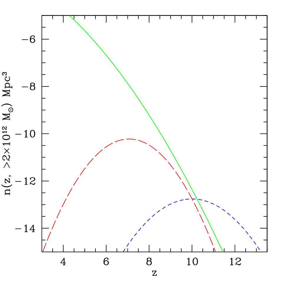
Ignoring the variation of the survey volume per redshift interval, the RPD for LBGs with luminosity at a wavelength of that is greater than within the volume observed in a given dropout band is given by,
| (1) |
where and are the mean and standard deviation of the given band, is the mass function of halos, and is a relation for the luminosity of an LBG contained in a halo of mass , which we describe in §5. Figure 1 shows how the PHSF is multiplied by the mass function to generate the real RPD for J-dropouts. In §6, we calculate the moments of this true distribution.
3 Moments of a Count of Objects
In this section we derive and discuss the formulae for the statistical moments of a count of halos above a given minimum mass, , in a given survey volume taking into account the variations of the mass and correlation functions along the light-cone. We limit the discussion to the first and second moments, and .
We generally follow Peebles 1980 in calculating moments of a count of objects in a box but augment the derivation by allowing the mass and correlation functions to vary with redshift. We begin by dividing the box into infintessimal units of size . The – unit in the box contains objects, so that the total number of objects in the box is . If every part of the box is viewed at the same cosmic time, then the average number of objects in each unit is obtained through the average number density of objects in the box: . However, if the box is viewed at some distance from the observer, then each unit sits at a particular redshift, and the average number of objects in units at redshift is related to the average number density of objects in the box at that redshift, . We assume that is small enough so that and the statistics of galaxies within each unit is Poisson distributed, i.e. at each redshift for every in .
We can now calculate the moments of a count of objects, N, in the box. The first moment is given by
| (2) | |||||
where the comoving volume element depends on the survey geometry. In the specific case of halos above a given mass threshold , is the mass function of halos above . Equation (2) is precisely what one would expect from simply integrating the mass function over the survey volume as in Naoz et al. 2006.
The second moment is
| (3) | |||||
If there is an object in each of the disjoint units and , the product is equal to unity. Otherwise, the product is equal to zero. The probability of both units containing an object is
| (4) |
where is the correlation between objects in units and . Thus, equation (3) reduces to
| (5) |
where
| (6) |
The variance of the count in the box can be expressed as,
| (7) |
can be thought of as the sum of a Poisson part, , and a clustering part, . In the specific case of halos above a given mass threshold, in equation (6) is the correlation function between halos with masses (possibly different) above at different redshifts, and is the mass function of such halos.
4 The Light-Cone Correlation Function
While several analytic prescriptions exist for calculating the correlation function of halos at different redshifts (Mo & White 1996; Porciani et al. 1998; Scannapieco & Barkana 2002), the correlation function measured in observations of LBGs is an average along the light-cone over the survey volume. The observed correlation between each halo with mass greater than and each other halo with mass greater than is (Matarrese et al. 1997):
| (8) | |||||
where
| (9) |
is the effective bias used to include halos at all masses above , is the mass autocorrelation function, is the halo mass function, is the bias factor, is the comoving distance between halos, and .
We use the reformulation of the correlation function on the light-cone given by Yamamoto & Suto 1999 which involves only a single integral:
| (10) |
While the mass function evolves extremely rapidly over the range of the PHSF, the evolution is minimal between two points separated by a distance, , small enough to produce a non-negligible correlation. This is the key approximation made by Yamamoto & Suto 1999 and hold well even in our regime.
5 A Model for High-Redshift Star-Forming Galaxies
To compare our results for the statistics of halos to those observed, we need a way of equating the mass of a halo, , with the luminosity of the observable galaxy it contains. In this section, we review a model given by Stark et al. 2007 that prescribes such a transformation for LBGs and LAEs.
The SLE07 model associates LBGs and LAEs with merger-activated star formation in dark-matter halos. The ratio of baryonic to dark matter mass in these halos is equal to the cosmic value, . The efficiency with which the baryons are converted into stars, denoted by , is a constant, , for halos more massive than a critical value . However, for halos below this mass, the feedback from supernovae suppresses star formation such that . Modeling and low-redshift observations suggest that corresponds to a velocity in the halo of (Dekel & Woo 2003; Kauffmann et al. 2003). We express the time-scale for star formation at as the cosmic time, , times the star formation duty cycle, . gives the fraction of the Hubble time during which the star formation occurs. The average star formation rate is then
| (12) |
For LBGs, the luminosity per unit frequency at a wavelength of is given by
| (13) |
assuming a Salpeter initial mass function (IMF) of stars.
For LAEs with a low metallicity (1/20 solar) and a Salpeter IMF one gets ionizing photons emitted per of star formation per year. A fraction of these photons do not escape from the galaxy and produce ions, of the resulting recombinations each produce a Lyman- photon with energy , and only a fraction these photons escape into and pass through the intergalactic medium to be observed. The Lyman- luminosity is then
| (14) |
where is the frequency of the Lyman- transition.
SLE07 fit the free parameters in their model ( and ) to observations at . For LBGs at , the best fit values and 1- errors are and . For LAEs at , and . These fit parameters are then used to determine the model at higher redshifts. We adopt this simple model with a fixed choice of its free parameters only as an illustrative example for relating the statistics of dark matter halos to observed galaxies. All of the plots given as functions of halo mass in the subsequent sections can be easily related to galaxy luminosities in the context of any more complicated models for galaxy formation and evolution.
6 Results
Next, we present the moments of the true RPD for i-, z-, and J-dropout LGBs in §6.1. Having derived expressions for the moments of halos counts in a survey volume and the correlation function for such halos along the light-cone in §6.2, we may compare these expressions quantitatively with those derived using a snapshot approach for various dropout surveys of LBGs in halos of different masses. The fractional variation does not depend on the survey field-of-view but only on the variation along the line-of-sight. Thus, our results apply to a wide variety of surveys for LBGs including the Great Observatories Origins Deep Survey (GOODS), the Hubble Ultra Deep Field (HUDF), and future surveys using the Subaru Multi-Object Infrared Camera and Spectrograph (MOIRCS) and the HST Wide Field Camera 3 (WFC3).
For our calculations, we use the mass function given by Sheth & Tormen 1999 and the bias factor in Sheth et al. 2001. Our results without the light-cone effect are produced by assuming that the entire volume exists at the mean redshift of the PHSF.
6.1 The Redshift Probability Distribution
Since the halos that host LBGs are rare at high redshifts and their abundance varies exponentially with redshift over the width of the PHSFs for dropout surveys, the RPD of LBGs in such a survey is biased toward lower redshifts. The low-redshift tail of a Gaussian PHSF exaggerates this effect. The true RPD, , is given by equation (1). The mean, variance, and skewness of the RPD are given by
| (15) |
| (16) |
and
| (17) |
The moments of the RPD for i-, z-, and J-band dropouts are shown in figures 2, 3, and 4. The plots show their dependence on halo mass, the broadness of the Gaussian shapes assumed for the PHSFs, and the cosmological parameter .


The most important difference between the PHSF and the RPD for a given band is in their means. The exponentially varying mass function biases the survey toward lower redshifts. The mean of the RPD is offset from that of the PHSF by an amount on the order of the PHSF’s standard deviation. Thus, in a J-dropout survey, the LBGs can be clustered around a redshift of as low as , depending on the luminosity of the galaxies considered, instead of being at .
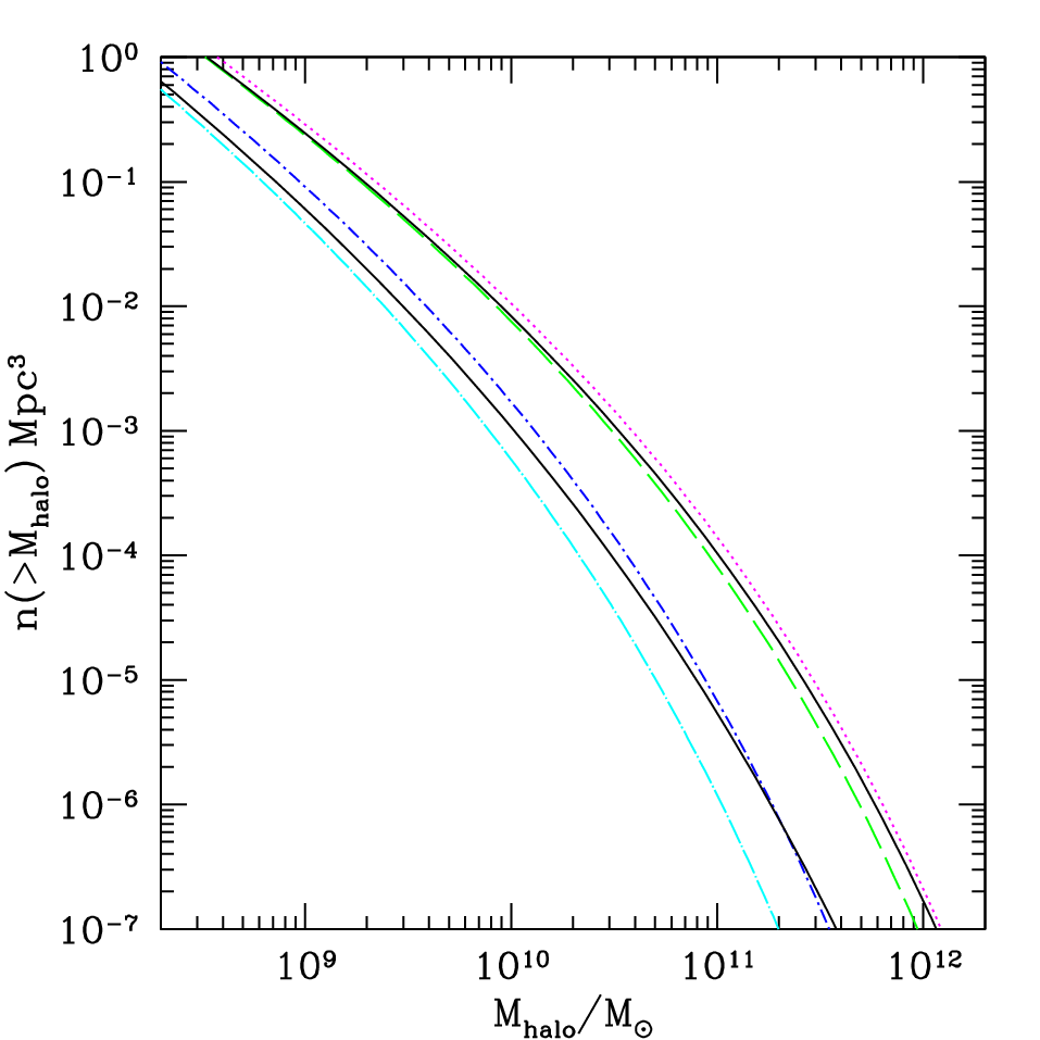
Another important point to extract from figure 2 is that the LBGs are segregated by their halo mass (luminosity) through the survey. Since the mean of the RPD decreases monotonically with halo mass (luminosity), the RPD for more luminous galaxies is shifted to lower redshifts than that of less luminous ones. While this series of RPDs overlaps, it is interesting to note that, for J-dropouts, galaxies in halos with and are almost completely unmixed since the means of their RPDs are about separated by about one rms variation. This has important implications for trying to reconstruct the mass function from observations since different masses are being observed at different redshifts. Consider halos in mass bins at two different masses, and , where , that are observed at two different redshifts, and , such that . The number of halos with is higher than it would be if these halos were seen at . Thus, the resulting inferred mass function is shallower than the true one determined using halos that are all at the same redshift. The effect is lessened by supression due to the PHSF, however. The density of halos of a given mass is less than the underlying density of such halos where they are seen at . Yet, their density is still higher than the underlying density at . The amplitudes of the mass function and the RPD at various redshifts can be compared for J-band halos with in figure 1. Figure 5 compares the extracted mass function with the underlying Sheth-Tormen mass function used to compute it.
The RPDs are slightly (by percent) narrower than the PHSFs. The normalized rms variation in the RPD as a function of the standard deviation of the PHSF is nearly identical for each band as are the equivalent plots as a function of halo mass for the i- and z- bands. This indicates that the slight narrowing is independent of the assumed standard deviation of the Gaussian PHSFs and depends only on the target redshift of a given band, i.e. the mean of its PHSF.
The asymmetry of the RPD is plotted in Figures 2, 3 and 4 as . The asymmetry is very small, on the order of tens of percent. This degree of symmetry and the fact that the skewness is positive might seem counter-intuitive since the exponentially varying mass function should bias the RPD toward lower redshifts. This bias, however, is manifested in the shift in the mean of the RPD away from that of the PHSF rather than in skewing the RPD. The Press-Schechter mass function with a simplified growth factor, , has two dependencies on redshift, a linearly increasing factor and an exponentially decaying one that dominates at high-redshift, , where and are independent of redshift. The exponential decay factor, however, is simply the tail of a Gaussian, which when multiplied by the Gaussian PHSF yields another symmetric Gaussian. Only the subordinate linear factor contributes to the asymmetry.
Finally, although changing the value of has a small effect on the value of the parameters we calculated, the difference as shown in Figure 4 was not drastic; all of the basic results we have just presented remain unchanged. In fact, the asymmetry of the RPD is virtually unchanged when is varied. This is consistent with the asymmetry being due only to the linear dependence on redshift, as discussed above, and not to the exponentially varying factor, which contains most of the mass function’s dependence on .
6.2 The Light-Cone Effect on Moments of Counts and the Correlation Function
As described above, the equations for the moments of the count of objects in the survey and their correlation are different if the light-cone effect is included. This effect is greatly enhanced by the wide PHSFs of the bands used in dropout surveys. For these surveys, the volume element in equations (2),(6), and (10) is replaced via
| (18) |
Figure 6 shows the results of including this effect on the mean count, clustering variance, and correlation function of halos containing the LGBs in i-, z-, and J-band dropout surveys. While the value of each of these statistics varies depending on the field-of-view of the particular survey under consideration, the fractional effect is independent of field-of-view since a change in the area of the survey is orthogonal to the variation in the mass and correlation functions along the lightcone.
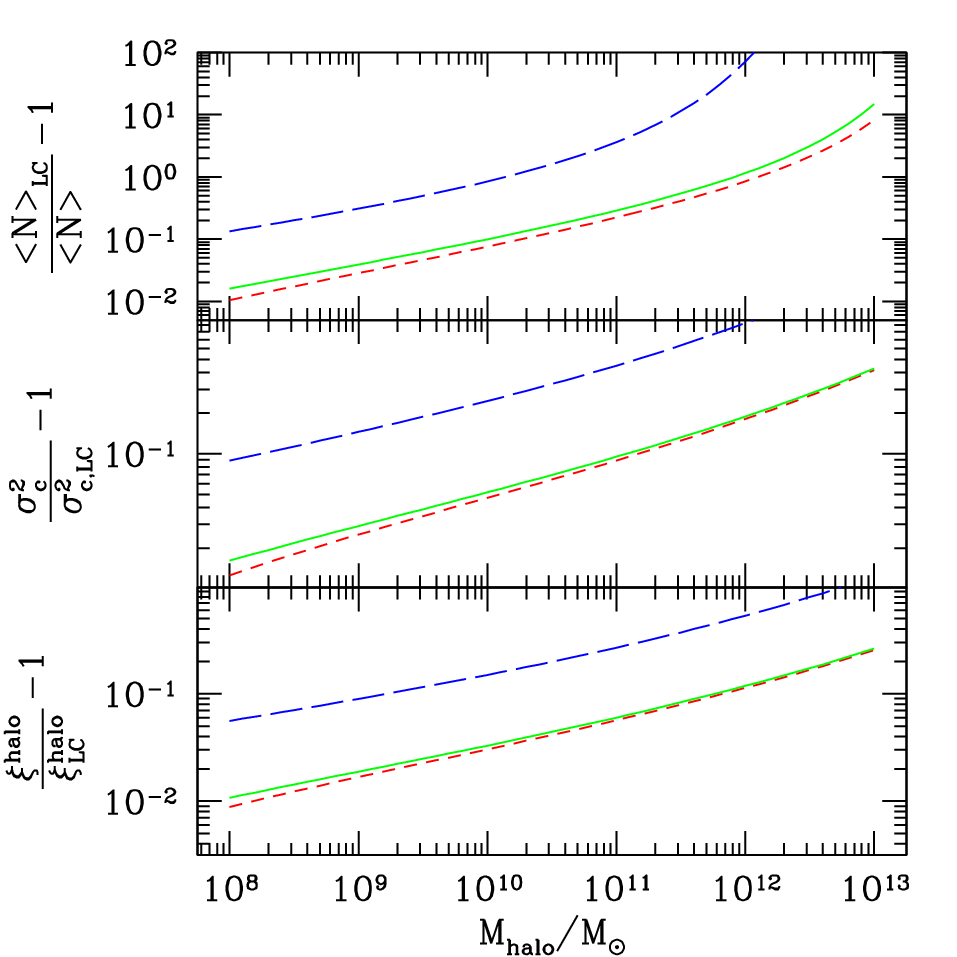
For i- and z-dropouts, the light-cone effect can make an order unity difference in the mean number of objects and a difference of roughly ten percent in the clustering variance of the count and the correlation (Eq. 10) at the high mass end. The effect for J-dropouts is much larger (by almost an order-of-magnitude) because the mass function has more evolution over the J-band both due to the increased steepness of the mass function at higher redshift and because the PHSF is much broader for the the J-band. The variation in the effect with halo mass is due to the mass segregation discussed in the previous section. In particular, the mass dependence of the effect on is manifested in the flattening of the mass function extracted from the survey shown in Figure 5.
In associating our calculations for the halo correlation function with LBGs, we note that the halos hosting LBGs do not constitute a fair sample of the entire halo population. Scannapieco & Thacker 2003 show through numerical simulations that these halos have undergone substantial accretion in their recent past giving them an extra “temporal” bias. While these simulations were performed at , there is as of yet no analytical method for predicting this extra bias at higher redshift. Since we compute only the fractional difference in the variance and correlation function, we are safe in ignoring this effect as long as the bias of LBGs over halos does not vary much within the redshift range of the RPD.
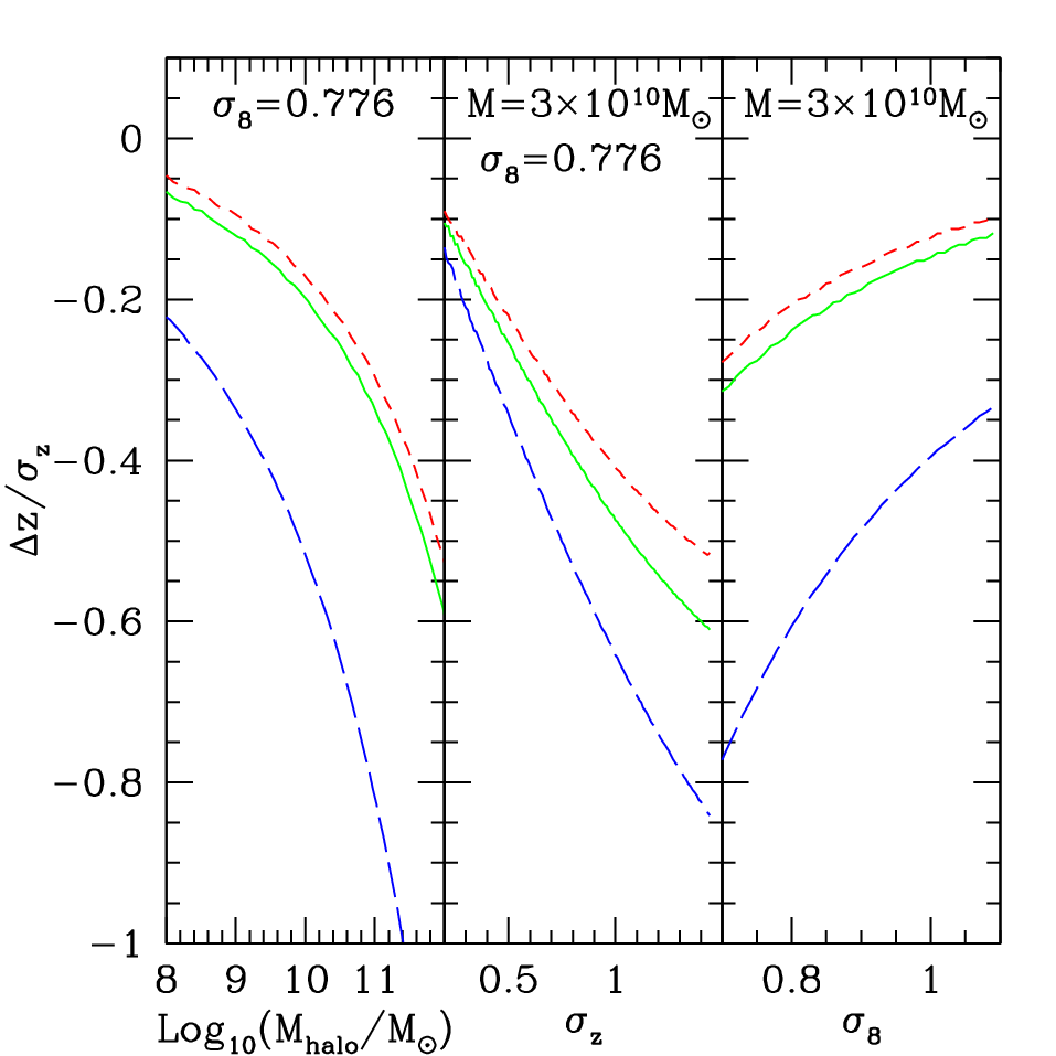
Finally, in §6.1 we showed that the LBGs in dropout surveys, which are more numerous than would be calculated ignoring the light-cone effect, are distributed at lower redshifts than indicated by the PHSF. However, it is also interesting to ask at what redshift does the “snapshot” calculation yield the same number of LBGs as the light-cone calculation. Hypothesizing a narrow-band survey for LBGs, this is equivalent to asking at what redshift does this hypothetical survey give the same density of LGBs as a dropout survey. The difference between this redshift and the mean of the PHSF is plotted in Figure 7 for each band.
7 Discussion
The variation of the mass function of halos along the light-cone within the volume of a dropout survey results in a mass segregation effect that is also manifested in their hosted LBGs. The observed sources are not at the mean of the photometric selection function (PHSF) but instead are distributed at lower redshifts (see Fig. 1). This effect applies to true LBG dropouts and ignores possible interlopers from lower redshifts whose spectra mimic those of higher redshift LGBs. The mass segregation results in different measured statistics of LBGs from those expected from theory or simulations along a space-like slice (snapshot) through the universe at the “mean survey redshift.” In particular, the mass/luminosity function extracted from such a survey is shallower than the underlying mass/luminosity function because of the different strengths of the light-cone effect on halos of different masses (LBGs of different luminosities). This flattening of the mass function is particularly important in the J-band because of its larger width in redshift space (see Fig. 5).
Without spectroscopic measurements to confirm the redshifts of a sample of LBGs, the mass segregation effect presents an added complication in continuing efforts to determine the effect of high-redshift LBGs on reionization (Nagamine et al. 2006; Stark et al. 2007) and the microwave background (Babich & Loeb 2007), or efforts to measure the high-redshift evolution of the star-formation rate (Sawicki & Thompson 2006; Ellis 2007). Reionization is a highly inhomogeneous process, and so the light-cone effect on the correlation function is also particularly relevant in that context (Barkana & Loeb 2004; Furlanetto & Loeb 2005). The lightcone effect on the measured correlation function of LBGs would also be important in attempts to use the clustering properties of LBGs to infer the masses of their host halos at higher redshift.
Dow-Hygelund et al. 2007 made an effort to follow up spectroscopically on LBGs from i-band dropout surveys near to measure their redshifts precisely. However, they were only able to confirm redshifts on 6 LBGs in their sample, a number insufficient to trace the RPD in a statistically significant way. Ando et al. 2004; Ando et al. 2007 preform similar studies on LBGs near , but the sample size they obtained was also not sufficiently large for this purpose. Ideally, one would like to perform this type of analysis on z- or J-band dropouts with the goal of tracing the RPD, but this would be very difficult both because of the present lack of candidates and because of the high integration times necessary with current technology.
8 Acknowledgements
We would like to thank Rychard Bouwens and Dan Stark for useful discussions. JM acknowledges support from a National Science Foundation Graduate Research Fellowship. This research was supported in part by Harvard University funds.
References
- Ando et al. (2007) Ando M., Ohta K., Iwata I., Akiyama M., Aoki K., Tamura N., 2007, ArXiv e-prints, 705
- Ando et al. (2004) Ando M., Ohta K., Iwata I., Watanabe C., Tamura N., Akiyama M., Aoki K., 2004, ApJ, 610, 635
- Babich & Loeb (2007) Babich D., Loeb A., 2007, MNRAS, 374, L24
- Barkana & Loeb (2004) Barkana R., Loeb A., 2004, ApJ, 609, 474
- Bouwens & Illingworth (2006) Bouwens R., Illingworth G., 2006, New Astronomy Review, 50, 152
- Bouwens et al. (2006) Bouwens R., Illingworth G., Blakeslee J., Franx M., 2006, ApJ, 653, 53
- Dekel & Woo (2003) Dekel A., Woo J., 2003, MNRAS, 344, 1131
- Dow-Hygelund et al. (2007) Dow-Hygelund C. C., Holden B. P., Bouwens R. J., Illingworth G. D., van der Wel A., Franx M., van Dokkum P. G., Ford H., Rosati P., Magee D., Zirm A., 2007, ApJ, 660, 47
- Ellis (2007) Ellis R. S., 2007, arXiv:astro-ph/0701024
- Furlanetto & Loeb (2005) Furlanetto S. R., Loeb A., 2005, ApJ, 634, 1
- Iye et al. (2006) Iye M., Ota K., Kashikawa N., Furusawa H., Hashimoto T., Hattori T., Matsuda Y., Morokuma T., Ouchi M., Shimasaku K., 2006, Nat, 443, 186
- Kauffmann et al. (2003) Kauffmann G., Heckman T. M., White S. D. M., Charlot S., Tremonti C., Peng E. W., Seibert M., Brinkmann J., Nichol R. C., SubbaRao M., York D., 2003, MNRAS, 341, 54
- Matarrese et al. (1997) Matarrese S., Coles P., Lucchin F., Moscardini L., 1997, MNRAS, 286, 115
- Mo & White (1996) Mo H. J., White S. D. M., 1996, MNRAS, 282, 347
- Mobasher et al. (2005) Mobasher B., Dickinson M., Ferguson H. C., 2005, ApJ, 635, 832
- Nagamine et al. (2006) Nagamine K., Cen R., Furlanetto S. R., Hernquist L., Night C., Ostriker J. P., Ouchi M., 2006, New Astronomy Review, 50, 29
- Naoz et al. (2006) Naoz S., Noter S., Barkana R., 2006, MNRAS, 373, L98
- Peebles (1980) Peebles P. J. E., 1980, The large-scale structure of the universe. Research supported by the National Science Foundation. Princeton, N.J., Princeton University Press, 1980. 435 p.
- Porciani (1997) Porciani C., 1997, MNRAS, 290, 639
- Porciani et al. (1998) Porciani C., Matarrese S., Lucchin F., Catelan P., 1998, MNRAS, 298, 1097
- Sawicki & Thompson (2006) Sawicki M., Thompson D., 2006, ApJ, 648, 299
- Scannapieco & Barkana (2002) Scannapieco E., Barkana R., 2002, ApJ, 571, 585
- Scannapieco & Thacker (2003) Scannapieco E., Thacker R. J., 2003, The Astrophysical Journal, 590, L69
- Scannapieco & Thacker (2005) Scannapieco E., Thacker R. J., 2005, ApJ, 619, 1
- Sheth et al. (2001) Sheth R. K., Mo H. J., Tormen G., 2001, MNRAS, 323, 1
- Sheth & Tormen (1999) Sheth R. K., Tormen G., 1999, MNRAS, 308, 119
- Spergel et al. (2007) Spergel D. N., Bean R., Doré O., 2007, ApJS, 170, 377
- Stark et al. (2007) Stark D. P., Ellis R. S., Richard J., Kneib J.-P., Smith G. P., Santos M. R., 2007, ApJ, 663, 10
- Stark et al. (2007) Stark D. P., Loeb A., Ellis R. S., 2007, arXiv:astro-ph/0701882v2
- Steidel et al. (1999) Steidel C. C., Adelberger K. L., Giavalisco M., Dickinson M., Pettini M., 1999, ApJ, 519, 1
- Yamamoto & Suto (1999) Yamamoto K., Suto Y., 1999, ApJ, 517, 1