The Yang-Mills Vacuum in Coulomb Gauge in DimensionsThanks: Supported in part by DFG under Re 856/6-1 and Re 856/6-2 and by the European Graduate School Basel-Graz-Tübingen
Abstract
The variational approach to the Hamilton formulation of Yang-Mills theory in Coulomb gauge developed by the present authors previously is applied to Yang-Mills theory in dimensions and is confronted with the existing lattice data. We show that the resulting Dyson-Schwinger equations (DSE) yield consistent solutions in dimensions only for infrared divergent ghost form factor and gluon energy. The obtained numerical solutions of the DSE reproduce the analytic infrared results and are in satisfactory agreement with the existing lattice date in the whole momentum range.
pacs: 11.10.Ef, 12.38.Aw, 12.38.Cy, 12.38.Lg
1 Introduction
Recently, there has been a renewed interest in the formulation of Yang-Mills theory in Coulomb gauge, both in the continuum theory [1, 2, 3, 4] and on the lattice [5, 6, 7, 8, 9]. In the continuum formulation the Hamilton approach turns out to be very appealing, in particular, for the description of the confining properties of the theory [3]. The reason is that in Coulomb gauge Gauss’ law can be explicitly resolved resulting in a static potential between color charges [10]. Recently, several papers have been devoted to a variational solution of the Yang-Mills Schrödinger equation in Coulomb gauge [2, 3, 4]. In particular, in refs. [3, 4] the present authors have developed a variational approach to Yang-Mills theory in Coulomb gauge which properly includes the curvature of the space of (transversal) gauge orbits. Using a Gaussian type of ansatz for the Yang-Mills vacuum wave functional minimization of the energy density results in a set of coupled Dyson-Schwinger equations which can be solved analytically in the infrared [1, 11] and has been solved numerically in the full momentum range [3, 21] in dimensions. An infrared divergent gluon energy and a linearly rising static quark potential was found [3, 21], both signaling confinement. Furthermore, within this approach the spatial ’t Hooft loop [22, 23] was calculated in the vacuum state and a perimeter law was found [20], which is the behavior expected for this disorder parameter in a confinement phase. In the present paper we apply this approach to dimensions and confront the results with the existing lattice data [9].
The dimensional Yang-Mills theory is interesting in several aspects: When a Higgs field is included, it represents the high temperature limit of the dimensional Yang-Mills theory, thereby the temporal component of the gauge field becomes the Higgs field in the dimensional reduced theory. In many respects the dimensional theory is easier to treat than its dimensional counter part, in particular, much larger lattices can be afforded in dimensions. This will be crucial for a comparison of the continuum results with the lattice data, since the lattices affordable in dimensions are by far too small to allow for a reliable extraction of the infrared properties of the Greens functions [12, 13]. In addition, dimensional Yang-Mills theory is super-renormalizable.
The balance of the paper is as follows: In section 2 we briefly summarize the essential ingredients of the Hamilton approach to Yang-Mills theory in Coulomb gauge [10] and of the variational solution of the corresponding Yang-Mills Schrödinger equation [3]. In section 3 the Dyson-Schwinger equations resulting from minimizing the energy density are studied in the ultraviolet and their renormalization is carried out. Some exact statements on their solutions are given in section 4, where we also solve these equations analytically in the infrared. In section 5 we present our numerical results and compare them with the existing lattice data. A short summary and some concluding remarks are given in section 6.
2 The Hamilton approach to Yang-Mills theory in Coulomb gauge
Canonical quantization of Yang-Mills theory is usually performed in Weyl gauge to avoid the problem arising from the vanishing of the canonical momentum conjugate to .11 1 An alternative to the Weyl gauge is the light-cone gauge . The prize one pays by choosing Weyl gauge is that one looses Gauss’ law as equation of motion. To ensure gauge invariance one has to impose Gauss’ law as a constraint on the wave functional. Instead of using gauge invariant wave functionals [14, 15, 16], it is simpler to explicitly resolve Gauss’ law by fixing the residual (time-independent) gauge invariance, and Coulomb gauge is a particularly convenient gauge for this purpose. After resolving Gauss’ law in Coulomb gauge the Yang-Mills Hamiltonian reads [10]
| (1) |
where
| (2) |
is the canonical momentum operator conjugate to the transverse gauge field . Furthermore
| (3) |
is the Faddeev-Popov determinant with being the covariant derivative in the adjoint representation. Furthermore
| (4) |
is the magnetic field, which is a scalar in dimensions (). Finally
| (5) |
is the non-Abelian Coulomb propagator which mediates a static interaction between the color charge density of the gluons
| (6) |
In the presence of external color charges, for example in the presence of quarks, their charge density has to be added to the gluon charge density. The kinetic term in the Hamilton has the form of a (variational extension of the) Laplace-Beltrami operator in curved space with the Faddeev-Popov determinant (3) corresponding to the determinant of the metric of the space of transversal gauge orbits. The Jacobian (3) also enters the scalar product in the Hilbert space of the Yang-Mills wave functionals in Coulomb gauge
| (7) |
We will solve the Yang-Mills Schrödinger equation by the variational principle
| (8) |
using the following ansatz for the vacuum wave functional [3], [4]
| (9) |
where is the variational kernel, which by translational and rotational invariance of the vacuum depends only on , and, by the isotropy of color space, is independent of color. The ansatz (9) with is motivated by the wave functional of a particle moving in a s-state in a spherically symmetric potential. In principle, could be used as a variational parameter to minimize the energy density. However, it turns out that up to two loops in the energy, stationarity of the energy density with respect to , i.e. , implies also stationarity with respect to , i.e. [4]. Thus, we are free to choose for convenience, and as in ref. [3] we will choose , which removes the Faddeev-Popov determinant from the integration measure in eq. (7). Furthermore with the choice the gluon propagator is given by
| (10) |
so that the Fourier transform has the meaning of the gluon energy.
The calculation of the vacuum expectation value of the Coulomb Hamiltonian in the state (9) proceeds in the same way as in 3+1-dimensions and we just quote the result. We find for the kinetic energy
| (11) |
the potential energy
| (12) | |||||
and for the Coulomb energy
| (13) | |||||
where with being the 2-dimensional spatial volume. Furthermore the quantity
| (14) |
is referred to as “curvature” of the space of gauge orbits. Introducing the ghost propagator by
| (15) |
with being the ghost form factor, the curvature (14) can be expressed as
| (16) |
Finally, denotes the Coulomb form factor, which is defined by
| (17) |
Minimization of the energy density results in the so-called gap equation, which can be cast into the form of a dispersion relation of a relativistic particle (gluon)
| (18) |
Here is an irrelevant constant which arises from the gluon tadpole. Furthermore, the quantity , which arises from the expectation value of the Coulomb term (13), can be expressed as
| (19) |
In principle or , and are defined uniquely once the trial wave functional is fixed. However, the exact evaluation of these expectation values (even with the above chosen trial wave function) is not feasible and one has to resort to further approximations. We shall adopt here the same approximation as in ref. [3] used in dimensions, approximating the full ghost-gluon vertex by its bare one. This approximation has been justified in Landau gauge [17] and, in fact, has received recently strong support by lattice calculations [18]. In this approximation the ghost and Coulomb form factors satisfy the following Dyson-Schwinger equations
| (20) |
| (21) |
| (22) |
| (23) |
As described in ref. [3] to the considered order (bare ghost-gluon vertex and 2-loop order in energy) the Coulomb form factor can be put .
In the coupling constant has the dimension of the square root the momentum and it is convenient to use the coupling constant to rescale all quantities by suitable powers of to render them dimensionless. The coupling constant then disappears from the Dyson-Schwinger equations. Denoting the dimensionless quantities by a bar we have
| (24) |
In the following we will skip the bar and, unless stated otherwise, all quantities will be understood as the dimensionless ones.
In section 4.1 we prove that for any solution of the coupled Dyson-Schwinger equations (18, 20) in the ghost form factor and the gluon energy are infrared divergent
| (25) | |||||
| (26) |
The first relation is the so-called horizon condition which had to be imposed ad hoc in but is a strict consequence of the Dyson-Schwinger equations in . The second condition (26) signals gluon confinement. In addition, we prove in appendix A that when the curvature is omitted, the coupled Dyson-Schwinger equations in do not allow for a consistent solution. This is again different from where the DSE allow for solutions with infrared finite when the curvature is ignored.
3 Ultraviolet behavior and renormalization
In the following we will investigate the ultraviolet behavior of the solutions of the Dyson-Schwinger equations and perform their renormalization, thereby following the procedure presented in refs. [3], [20] for the -dimensional case. Since most of the considerations will parallel the -dimensional case we will be very brief.
For the uv-analysis it is sufficient to use the angular approximation
| (27) |
The angular integral in the ghost Dyson-Schwinger equation and also in the curvature then becomes trivial and we obtain for the corresponding momentum integrals
| (28) | |||||
| (29) |
The asymptotic analysis of the Dyson-Schwinger equations is simplified by taken the derivative with respect to the external momentum
| (30) | |||||
| (31) |
As we will see below, the remaining momentum integrals are ultraviolet convergent22 2 The ghost integral is uv-finite as will be shown later.. The derivative of the ghost Dyson-Schwinger equation (20) yields
| (32) |
where
| (33) |
and the derivative of the curvature (16) yields
| (34) |
where
| (35) |
We now discuss the ultraviolet behavior of the relevant quantities.
3.1 Ultraviolet behavior
For large momenta the term on the r.h.s. of the gap equation (18) dominates [3] and the gluon energy behaves like
| (36) |
in accordance with asymptotic freedom. This behavior will in fact be confirmed by the numerical solutions presented in section 6. Assuming (36), we will investigate the uv-behavior of the remaining quantities: the ghost form factor , the curvature and the Coulomb form factor .
For large the -dependence of the integral (33) is independent of the infrared behavior of and with eq. (36) we find
| (37) |
and the derivative of the ghost DSE (32) reduces to
| (38) |
To solve this equation, let us assume for the moment for . Then the differential equation (38) reduces to
| (39) |
whose solution is given by
| (40) |
where is an integration constant. Indeed, for large this solution satisfies . To determine the integration constant , we consider the asymptotic behavior of the integral (28) for , where and . This yields
| (41) |
Since , we obtain from the DSE of the ghost form factor , which fixes the integration constant in eq. (40) to , so that the asymptotic form of the ghost form factor becomes
| (42) |
Accordingly we find for the unscaled form factor33 3 Below we denote the dimensionful (unscaled) quantities by a ”tilde”. the asymptotic form
| (43) |
From the Swift relation [19], [3]
| (44) |
we find for the Coulomb form factor
| (45) |
which obviously has the same asymptotic form as the ghost form factor.
With the asymptotic behavior of the ghost (42), we find for the derivative of the curvature (34)
| (46) |
and for the integral (35)
| (47) |
so that
| (48) |
i.e.
| (49) |
Accordingly, the ratio
| (50) |
vanishes in the ultraviolet implying that the space of gauge orbits becomes asymptotically flat in accordance with asymptotic freedom.
3.2 Renormalization
With the above obtained uv-behavior (see eqs. (36), (42) and (45)) the integrals (21) and (23) are uv-convergent. Thus, contrary to the dimensional case in the DSE for the ghost and Coulomb form factors do not need renormalization. What needs, however, renormalization is the curvature and the gap equation. The renormalization of these two equations is carried out in exactly the same way as described in refs. [20] and [3], i.e. basically by subtracting this equations at a renormalization point , which leads to the renormalized equations [20]
| (51) | |||||
| (52) |
Here and
| (53) |
are finite renormalization constants. Furthermore, we have introduced the abbreviation
| (54) |
with
| (55) |
Note, since the ghost equation needs no renormalization, there are only three renormalization constants , and and furthermore, the solutions of the coupled ghost and gluon DSEs do not depend on 44 4 Some observables like the ’t Hooft loop (in ) do, however, depend on [20].. (Note the integrals (55) depend only on the finite quantity but not on the renormalization constant [20].) One of the two independent renormalization constants, , is used to implement the horizon condition . As will be shown in the next section any consistent solution of the coupled DSEs does satisfy this condition. The remaining renormalization constant can be chosen at will and determines the infrared limit of the wave functional as will be shown at the end of the next section.
4 Analytic results
The Dyson-Schwinger equations arising from the variational solution of the Schrödinger equation have in principle the same form in as in dimensions. However, due to the fact that the dimensional theory is superrenormalizable some rigorous properties of the solution of the Schwinger-Dyson equations can be derived which are not accessible in dimensions. Below we shall derive some rigorous properties of the solutions of the DSE and discuss their physical implications.
4.1 General results
Consider the ghost DSE (20). Since the integral (21) is convergent in (unlike in ), the ghost DSE needs no renormalization and thus no renormalization constant is introduced by this equation. It is then not difficult to prove the following statement:
If is a continuous function in , it satisfies
| (56) |
We prove the statement by reductio ad absurdum: Assume for all . Then, since by normalizability of the wave functional it follows from (21) and thus from the ghost DSE (20)
| (57) |
in contradiction to the assumption. Hence, cannot be negative everywhere. Assume now there exist some momentum for which . Since as a solution of the DSE, can be assumed to be continuous and as shown above is not everywhere negative, it must have at least one zero, say , i.e. , where changes sign. By the ghost DSE, eq. (20) has to be singular at and change sign at , too. However, changing integration variable in the (convergent!) integral (21) we find
| (58) |
and by the positivity of , and have the same sign in contradiction to the above assumption. Thus, holds for all . Then from eq. (21) follows and by the ghost DSE (20) . Note, that (56) is also in agreement with the asymptotic uv-behavior found in the previous section.
Assume now that the ghost form factor is bounded from above, i.e. there exist some upperbound such that for . According to (56) is then restricted to the intervall and the integrand in (16) is positive definite. Therefore, replacing in the curvature (16) by its upper and lower bound, we obtain an upper and lower bound to
| (59) |
where we have introduced a momentum cutoff since the integral is uv-divergent. The angular integral can be done analytically55 5 Note that this exact relation is also reproduced by the angular approximation.
yielding
| (63) |
Inserting this result into eq. (59), we find for the bounds
| (64) |
Note that this relation holds for all . In particular, this relation shows that is infrared divergent
| (65) |
For an infrared divergent the gap equation (51) reduces in the infrared to (see also ref. [20])
| (66) |
where is the renormalization constant introduced in eq. (3.2). Eq. (66) shows that has the same infrared behavior as . Thus, if the ghost form factor is bounded the gluon energy is logarithmically infrared divergent . It is now not difficult to show that with such an infrared behavior of the ghost Dyson-Schwinger equation does not possess a solution. To show this let us assume that there exist an such that
| (67) |
with some positive constant , which includes the case (65). Consider the integral in the ghost Dyson-Schwinger equation (21)
| (68) |
Since , see eq. (56), we obtain the following estimate
| (69) |
The angular integral can be done exactly using eq. (4.1) resulting in
| (70) |
Inserting here eq. (67) we obtain
| (71) |
Thus we find
| (72) |
and from the ghost Dyson-Schwinger equation (20) follows , which is in contradiction to the rigorous result (56). Thus we have shown that the coupled ghost and gluon Dyson-Schwinger equations do not allow for a ghost form factor which is bounded from above. We now show that ghost form factor is a monotonously decreasing function of , i.e.
| (73) |
for all finite .
As shown above in the ultraviolet analysis for . Assume now, as we lower , at some finite , . Then from the eq. (30) follows , which is in contradiction to the ghost DSE from which follows
| (74) |
Thus (73) holds in the whole momentum range. Since (56) and is monotonously decreasing in the whole momentum range and furthermore must not be bounded from above, it follows that is infrared divergent, i.e.
| (75) |
which is the horizon condition.
This is different from the dimensional case where solutions to the Dyson-Schwinger equation exist with an infrared finite ghost form factor.
4.2 Infrared analysis
The DSE can be solved analytically in the infrared completely analogous to the dimensional case. For this purpose we make the following power ansätze in the infrared
| (76) |
We will first resort to the angular approximation used already in the uv-analysis. Later on we will present the results obtained without resorting to the angular approximation.
With the infrared ansätze (76), we find for the integrals defined by eq. (33) and (35)
| (77) |
From the derivative of the ghost DSE (74) we obtain
| (78) |
which implies
| (79) |
and
| (80) |
In an analogous fashion we obtain from the derivative of the curvature
| (81) |
resulting in
| (82) |
and
| (83) |
From eq. (79) and (82) follows
| (84) |
showing that and have the same infrared exponents just like in the dimensional case (ref. [3]). In fact, follows already from the infrared limit of the gap equation (66). From this equation in addition follows that not only the infrared exponents but also the prefactors of both quantities have to coincide, i.e.
| (85) |
Dividing eq. (80) by (83) and using (84) we obtain
| (86) |
and
| (87) |
As we will see in sect. 6, this infrared behavior yields a linearly rising static color Coulomb potential provided we approximate the Coulomb form factor by its leading term which is correct to the order considered in the present paper.
The infrared analysis of the Dyson-Schwinger equations can be also carried out without resorting to the angular approximation. In fact, in ref. [11] the infrared analysis was carried out for arbitrary dimensions. In that case one finds from the ghost DSE the following sum rule for the infrared exponents
| (88) |
due to the non-renormalization of the ghost-gluon vertex. As shown in ref. [11] this sum rule guarantees that and have the same infrared exponent as already found above in the angular approximation, and in agreement with the infrared limit of the gap equation (66). Eq. (66) together with the ghost DSE in the infrared limit can be solved analytically for the infrared exponents yielding [11]
| (89) |
which is somewhat smaller than the infrared exponent found above in the angular approximation (87).
The above given infrared analysis is independent of the so far unfixed renormalization constants and . (Recall that the coupled set of DSEs (20), (51), (52) do not depend on .) From eq. (66) we obtain
| (90) |
If one uses the infrared expressions for defined by eq. (76), one finds that the energy density is minimized for (see ref. [20]). Using the representation [4]
| (91) |
which is correct to the order considered in the present paper, implies an infrared limit of the wave functional
| (92) |
This wave functional describes a stochastic vacuum, where the infrared modes of the gauge field are completely unconstrained.
5 Numerical results
The coupled DSEs (16), (20), (22), (52) were solved numerically in the whole momentum range as described in refs. [3] and [21]. The renormalization constant was fixed by implementing the horizon condition . Furthermore, like in the dimensional case in order to stay consistently in 1-loop approximation we have solved the equation for the Coulomb form factor by assuming a bare ghost form factor in the DSE for .


The numerical results obtained are presented in figs. 1 and 2. Fig. 1 shows the gluon energy and the curvature . Both quantities are infrared divergent and approach each other for in agreement with our infrared analysis given in the previous section. Fig. 2 shows the ghost and the Coulomb form factor. The ghost form factor is of course infrared divergent, since as shown in sect. 4, self-consistent solution of the Dyson-Schwinger equations exist only for infrared divergent ghost form factors. The Coulomb form factor is infrared finite and approaches asymptotically for the ghost form factor.


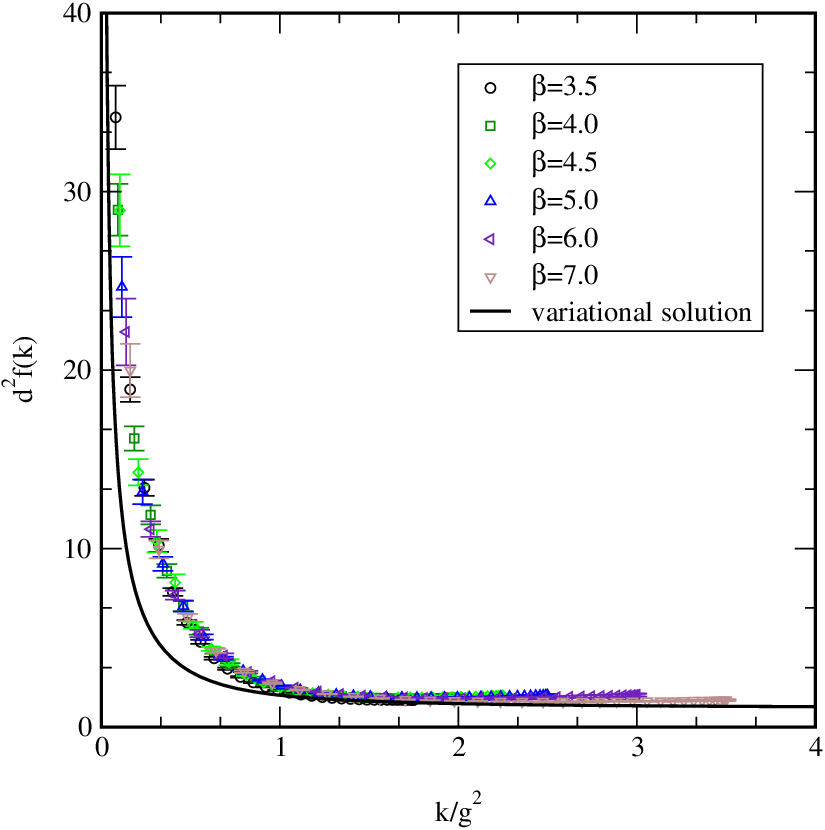
Fig. 3 shows the static color Coulomb potential defined by [3]
| (93) |
where is the (ordinary) zero’th order Bessel function. For the infrared behavior obtained in the angular approximation , see eq. (76), , which leads to a strictly linearly rising quark potential at large distances, while for , where the potential behaves as and we obtain the familiar Coulomb potential in dimensions. The infrared analysis carried out without resorting to the angular approximation yields . A careful analysis of our numerical solutions (obtained without the angular approximation) yields , which is in between the analytical results obtained with and without the angular approximation. In figs. 4, 5 and 6 we compare our numerical results for the ghost form factor , the gluon energy and the form factor of the Coulomb potential with the lattice data. It has been shown by solving the Dyson-Schwinger equation in Landau gauge on the torus [12], [13], that very large lattices are required to capture the correct infrared behavior of the Greens functions of the continuum theory. While these lattice sizes can be reached in 3 dimensions, they are out of reach in . The lattice calculations performed in ref. [9] in dimensions used lattices of the size , which should be sufficient to extract the correct infrared limit of the Greens functions. Our numerical results obtained by solving the DSE in Coulomb gauge are in quite satisfactory agreement with the lattice data. In particular, the asymptotic ultraviolet and infrared behaviors are quite well reproduced.
6 Summary and Conclusions
We have performed a variational solution of the Yang-Mills Schrödinger equation in Coulomb gauge in . The Dyson-Schwinger equations resulting from the minimization of the vacuum energy density have been solved analytically in the ultraviolet and in the infrared and in addition some rigorous results of their properties have been derived. In particular, we have shown that the ghost form factor as well as the gluon energy have to be infrared divergent, which is different from the dimensional case where solutions of the DSEs exist with these quantities being infrared finite [24]. The static non-Abelian Coulomb potential resulting from our numerical solution of the DSE is almost linearly rising. Our numerical results are in satisfactory agreement with the existing lattice data. The lattice calculations performed in so far use too small lattices to give reliable results for the continuum limit, in particular, on the infrared properties of the various Green’s functions [12], [13].
Acknowledgments
Discussions with G. Burgio, D. Epple, M. Quandt, W. Schleifenbaum, A. Szczepaniak and A. Weber are gratefully acknowledged.
References
- [1] D. Zwanziger, Phys. Rev. D 70 (2004) 094034 [arXiv:hep-ph/0312254].
- [2] A. P. Szczepaniak and E. S. Swanson, Phys. Rev. D 65 (2001) 025012 [arXiv:hep-ph/0107078]; A. P. Szczepaniak, Phys. Rev. D 69 (2004) 074031 [arXiv:hep-ph/0306030].
- [3] C. Feuchter and H. Reinhardt, Phys. Rev. D 70 (2004) 105021 [arXiv:hep-th/0408236], arXiv:hep-th/0402106.
- [4] H. Reinhardt and C. Feuchter, Phys. Rev. D 71 (2005) 105002 [arXiv:hep-th/0408237].
- [5] J. Greensite, S. Olejnik and D. Zwanziger, Phys. Rev. D 69 (2004) 074506 [arXiv:hep-lat/0401003].
- [6] K. Langfeld and L. Moyaerts, Phys. Rev. D 70 (2004) 074507 [arXiv:hep-lat/0406024].
- [7] S. Furui and H. Nakajima, arXiv:0708.1421 [hep-lat].
- [8] A. Cucchieri and D. Zwanziger, Phys. Rev. D 65 (2002) 014001 [arXiv:hep-lat/0008026].
- [9] L. Moyaerts, PhD thesis, University of Tübingen.
- [10] N. H. Christ and T. D. Lee, Phys. Rev. D22 (1980) 939; Phys. Scripta 23 (1981) 970.
- [11] W. Schleifenbaum, M. Leder and H. Reinhardt, Phys. Rev. D 73 (2006) 125019 [arXiv:hep-th/0605115].
- [12] C. S. Fischer, R. Alkofer and H. Reinhardt, Phys. Rev. D 65, 094008 (2002) [arXiv:hep-ph/0202195].
- [13] C. S. Fischer, A. Maas, J. M. Pawlowski and L. von Smekal, arXiv:hep-ph/0701050.
- [14] K. Johnson, The Yang-Mills Ground State, Proceedings of the workshop “QCD - 20 Years Later”, Aachen, 1992, edited by P.M. Zerwas and H.A. Kastrup, Vol 7; D.Z. Freedman, P.E. Haagensen, K. Johnson, and J.-I. Latorre, hep-th/9309045; N, Bazer, D.Z. Freedman, and P.E. Haagensen, Nucl. Phys. B428, 147 (1994)
- [15] I.L. Kogan and A. Kovner, Phys. Rev. D 52, 3719 (1995); C. Heinemann, C. Martin, E. Jancu and D. Vautherin, Phys. Rev. D 61 116008 (2000); O. Schröder and H. Reinhardt, Ann. Phys. (N.Y.) 312 319 (2004); O. Schröder and H. Reinhardt, Ann. Phys. (N.Y.) 307 452 (2003)
- [16] J. Greensite, S. Olejnik, arXiv:0707.2860 [hep-lat]
- [17] J.C. Taylor, Nucl. Phys. B33 (1971) 436
- [18] A. Maas, Phys. Rev. D 75, 116004 (2007) [arXiv:0704.0722 [hep-lat]].
- [19] A. R. Swift, Phys. Rev. D38 (1988) 668
- [20] H. Reinhardt and D. Epple, Phys. Rev. D76 (2007) 065015, arXiv:0706.0175 [hep-th].
- [21] D. Epple, H. Reinhardt and W. Schleifenbaum, Phys. Rev. D 75 (2007) 045011 [arXiv:hep-th/0612241].
- [22] G. ’t Hooft, Nucl. Phys. B 138, 1 (1978).
- [23] H. Reinhardt, Phys. Lett. B 557, 317 (2003) [arXiv:hep-th/0212264].
- [24] D. Epple, H. Reinhardt, W. Schleifenbaum and A. Szczepaniak, in preparation