Renormalized Polyakov loops in many representationsPreprint: BI-TP 2007/30, BNL-NT-07/45 and TIFR/TH/07-30
Abstract
We present a renormalization procedure for Polyakov loops which explicitly implements the fact that the renormalization constant depends only on the ultraviolet cutoff. Using this we study the renormalized Polyakov loops in all representations upto the 27 of the gauge group SU(3). We find good evidence for Casimir scaling of the Polyakov loops and for approximate large- factorization. By studying many loops together, we are able to show that there is a matrix model with a single coupling which can describe the high temperature phase of QCD, although it is hard to construct explicitly. We present the first results for the non-vanishing renormalized octet loop in the thermodynamic limit below the SU(3) phase transition, and estimate the associated string breaking distance and the gluelump binding energy. By studying the connection of the direct renormalization procedure with a generalization of an earlier suggestion which goes by the name of the renormalization procedure, we find that they are functionally equivalent.
pacs
11.10.Gh, 11.10.Wx, 11.15.Ha, 11.15.Pg, 12.38.Gc, 12.38.Mh, 25.75.NqI Introduction
The proof of confinement in QCD is now literally a million dollar question
clay. There are many ideas about the direction in which such
a proof lies. No matter what these ideas are, once they are properly
formulated, they are always open to test by lattice techniques. One of
the long-lasting ideas has been to examine a toy model of QCD for large
number of colors, tHooft:1973jz. Because of the enhanced symmetry,
many quantities become amenable to study in this limit. Computations of
corrections upto sub-leading order, , have been made for quantities
such as hadron masses and pion-nucleon scattering, with intriguing
results. Recently, by adding supersymmetries to large- QCD, very simple toy
models have been constructed which are amenable to analytical treatment
using the AdS/CFT correspondence Policastro:2001yc. Much excitement has
been generated by the plethora of predictions of such toy models, and
there have been exciting speculation about their applicability to QCD.
At large the dynamics of quarks is secondary to that of the gluons,
being suppressed by power corrections in . Hence lattice tests of
these ideas have been made in pure gauge, or quenched, QCD. There have
been investigations of the string tension and its scaling with
Bringoltz:2006zg, the nature of the phase transition with changing
Lucini:2003zr, and tests of approximate scale-invariance of finite
temperature QCD Gavai:2004se. In this paper we investigate certain
ideas about Polyakov loops and their behavior at finite temperature
which have developed in recent years based on large and the AdS/CFT
correspondence. We investigate matrix models which could be expected to
describe the high temperature phase of pure gauge QCD. Our results put
very strong constraints on the kinds of matrix models which may provide
a description of pure gauge QCD.
The Polyakov loop is closely connected with
confinement since it is the order parameter for
the transition from a confined to a
deconfined medium.
Various models based on Polyakov loops have been proposed to
describe the transition to a quark gluon plasma phase and its properties at
zero as well as non-zero baryon density
Pisarski:2006hz; Dumitru:2003hp; Dumitru:2004gd; Dumitru:2005ng; Dumitru:2003cf; Megias:2005ve; Megias:2004hj; Ratti:2005jh; Meisinger:2003id; Fukushima:2003fm; Diakonov:2004kc; Schaefer:2007pw; Blaschke:2007np; Ghosh:2007; Kashiwa:2007hw.
Furthermore the connection of SU(3) theory to the
large limit, in the mean-field approximation, was discussed in
Dumitru:2003hp; Dumitru:2004gd.
For a test of the reliability and comparison of these Polyakov loop models to
pure gauge theory and QCD with dynamical quarks, a detailed knowledge of the
behavior of the Polyakov loop in the fundamental and higher
representations in those theories is needed.
The Polyakov loop needs to be renormalized, since it has divergent
contributions from the ultraviolet. In Section III
we present a renormalization procedure which explicitly incorporates
properties expected of a good scheme. This direct renormalization
technique is naturally applicable to Polyakov loop expectation
values in all representations of the color group. The multiplicative
renormalizations in different representations are closely connected if
the Polyakov loops satisfy a property called Casimir scaling. We present
tests of Casimir scaling in Section IV. This leads on,
in Section V, to a test of large- factorization at
. We find good evidence for both in a temperature range not too
close to .
Next, in Section VI, we examine whether the renormalized
Polyakov loops are described in an effective matrix
model. By examining the renormalization scheme dependence of these
quantities, we find that a single parameter variation of matrix models
describes the temperature dependence of the Polyakov loops in various
representations. We also show that the matrix model is unlikely to consist
of a small set of terms, and therefore hard to construct explicitly from
the phenomenology of Polyakov loops.
In Section VII we consider the adjoint Polyakov
loop correlations below . We report the first measurement of the
renormalized adjoint Polyakov loops in the thermodynamic limit at finite
temperature in the confined phase of QCD. We find that aspects of the
adjoint Polyakov loop correlations can be summarized in the physics of
gluelumps, i.e., colorless states made of static adjoint sources and glue.
In the appendices we consider a renormalization procedure, the procedure, earlier suggested in Kaczmarek:2002mc. We
extend it to the renormalization of Polyakov loops in arbitrary
representations, consider the relation between the direct and renormalization procedures, and examine “color averaged” Polyakov
loop correlators in various representations.
II Details of the calculations
We have performed simulations for temperatures up to
on
lattices with and
up to 32 in SU(3) pure gauge
theory with the tree level Symanzik-improved gauge action
Weisz:1982zw; Weisz:1983bn.
We used a pseudo heatbath algorithm with FHKP updating in the SU(2)
subgroups. Each heatbath update was followed by four overrelaxation steps.
The statistics varies from 1000 to 10000 of such sweeps after suitable
thermalization.
The physical scale has been set using the zero temperature string tension,
, Beinlich:1997ia
and a determination of the critical coupling for the deconfinement transition
from Beinlich:1996xg.
We have calculated the Polyakov loops in all representations up to using
the operators defined in (41)-(47).
The errors on the observables were determined with the Jackknife method.
Furthermore, we have reanalyzed
configurations generated using two flavors of staggered quarks with mass on
a lattice at several temperatures above and below the
transition temperature Allton:2002zi; Allton:2003vx. At each temperature we have used
statistics of several thousands to
calculate Polyakov loops up to .
III Renormalization of Polyakov loops
We define the thermal Wilson line, at spatial position as
| (1) |
where is the gauge link matrix in the time direction at the point and Euclidean time . is a matrix which belongs to . We define the local Polyakov loop as the trace of ,
| (2) |
where the trace is normalized to one. We denote the expectation value of the Polyakov loop in the fundamental representation of SU(3) by
| (3) |
Polyakov loops in different representations, , are defined in Appendix A. The subscript indicates the dimension of the color (irreducible) representation of the Polyakov loop, e. g., for fundamental or for adjoint. Expectation values of Polyakov loops are ultraviolet divergent. We will use the superscripts or for bare and renormalized Polyakov loop respectively.
III.1 Basic properties of renormalization
It was pointed out by Polyakov Polyakov:1980ca that for smooth loops, ultraviolet divergences can be absorbed in the charge renormalization of gauge fields:
| (4) |
where is the length of the contour and the coupling, , on the right is the
bare coupling. The quantity on the left is properly renormalized and depends on the
renormalized coupling or, through this running coupling, on the temperature.
Cusps and self intersections of loops give rise to
logarithmic divergences which depend, e. g., on the angle
of the cusps Polyakov:1980ca; Dotsenko:1979wb; Korchemsky:1987wg.
Spatial averages of operators such as , which wind
times around the lattice, also need separate renormalization. Similarly,
composite operators such as powers of Polyakov loops,
including Polyakov loop susceptibilities, also
require independent renormalization.
We have written eq. (4) for
an arbitrary representation . The renormalization constants in different
representations, , can be related to each other if
both the bare and the renormalized loops satisfy the relation
| (5) |
called Casimir scaling. Here is the quadratic Casimir operator in the representation . When Casimir scaling holds, the quantities
| (6) |
where , are all equal.
In keeping with the general form in eq. (4) we can write
| (7) |
where the renormalization constants should only depend on the bare coupling. Such a multiplicative renormalization is expected to compensate entirely for the dependence of the bare loop on the cutoff, i.e., the bare coupling, so that the renormalized loop on the left is a function only of the temperature. Furthermore, if Casimir scaling is found to hold, then all the collapse to a single function , i.e. loops in all representations can be simultaneously renormalized. Note that there is one remaining ambiguity: the function can be multiplied by a single coupling independent constant without affecting the renormalization. Thus, a one parameter family of renormalization schemes for Polyakov loops is defined by eq. (7).
III.2 Direct renormalization of the Polyakov loop


In this subsection we present a complete renormalization procedure which
implements eq. (7). We call this the direct renormalization
prescription. A similar procedure was discussed
earlier in Creutz:1980hb. Denote by the Polyakov
loop expectation value obtained after taking the thermodynamic limit
at a temperature , where is the lattice spacing
at a bare coupling and is the temporal extent of the
lattice. We will describe the procedure for a fundamental loop first.
First choose the value of , at a reference temperature
. It is clear from eq. (7) that this choice is
exactly equivalent to fixing the renormalization scheme. It is convenient,
but not necessary, to take to be the maximum temperature in
the study: in our case . We discuss our choice of scheme
in Appendix C. This sets the first step of the iterative
procedure starting at the initial temperature .
Next we need measurements at (at least) two different temporal
extents, and , say, with
, both at the temperature
(we begin with and set up an iteration). Therefore these
measurements correspond to two different lattice cutoffs
with
, where the subscripts are self-explanatory.
We obtain two different renormalization constants,
| (8) | |||||
| (9) |
The third step is to advance the iteration. We do this by making a measurement of on the lattice with temporal extent at a temperature . Since the renormalization constant is already known from eq. (9), one obtains the value of
| (10) |
Since we have the value of the renormalized loop at a new temperature,
we can now iterate the procedure from the second step on. The iteration
gives the renormalized loops and the renormalization constants at a
decreasing series of temperatures.
Four points about the prescription are worth noting explicitly.
First, the procedure extends without change to any representation
. The test of Casimir scaling would be to assume that the bare
loops in different representations at are related by eq. (5), and then check whether the renormalized loops
at all are related in the same way. We discuss this further in
Section IV. Second, in the confined phase of
the pure gauge theory the bare Polyakov loop, in any representation
with non-vanishing triality, vanishes in the thermodynamic limit;
as a result the direct renormalization procedure can only be used
above for such representations. Third, a reverse iteration can
always be performed by choosing . Finally, although we discussed
the procedure for two values of , it can be easily extended to
a larger number of values for the temporal extent.
The renormalized Polyakov loop in the fundamental representation
obtained by the direct procedure described here is shown in Figure
1. Also shown, for comparison, are the results
obtained from a completely different renormalization procedure
Kaczmarek:2002mc based on a matching of the short distance behavior
of heavy quark-antiquark free energies to the zero temperature potential
(labeled as -renormalization). Both these procedures allow
a one parameter family of renormalization schemes, and the schemes
have been chosen so that the value of match.
Figure 2 shows the results for the renormalization
constant. These figures indicate the functional equivalence of the two
renormalization procedures.
III.3 Fundamental Polyakov loops


| 4 | 1.012 | 0.4070(11) | 4 | 6.001 | 1.0897(4) |
| 4 | 1.031 | 0.4600(7) | 4 | 8.002 | 1.0986(5) |
| 4 | 1.049 | 0.4927(22) | 4 | 10.00 | 1.1011(7) |
| 4 | 1.099 | 0.5649(14) | 4 | 12.13 | 1.1014(6) |
| 4 | 1.144 | 0.6049(3) | 4 | 14.00 | 1.1000(3) |
| 4 | 1.151 | 0.6114(16) | 4 | 16.00 | 1.0988(6) |
| 4 | 1.200 | 0.6494(12) | 4 | 18.01 | 1.0966(5) |
| 4 | 1.241 | 0.6759(15) | 4 | 20.00 | 1.0954(8) |
| 4 | 1.301 | 0.7095(13) | 4 | 22.00 | 1.0939(10) |
| 4 | 1.499 | 0.7953(13) | 4 | 24.00 | 1.0924(12) |
| 4 | 1.549 | 0.8115(8) | |||
| 4 | 1.600 | 0.8288(9) | 8 | 1.03 | 0.4818(99) |
| 4 | 1.684 | 0.8523(2) | 8 | 1.18 | 0.6330(125) |
| 4 | 2.214 | 0.9475(3) | 8 | 1.48 | 0.7763(116) |
| 4 | 2.858 | 1.0087(1) | 8 | 2.95 | 1.0149(68) |
| 4 | 2.999 | 1.0169(1) | 8 | 6.00 | 1.0961(33) |
| 4 | 3.987 | 1.0591(2) | 8 | 9.00 | 1.1049(27) |
| 4 | 5.001 | 1.0791(2) | 8 | 12.00 | 1.1060(26) |
| 4 | 0.90294 | 1.2144(2) | 4 | 1.47783 | 1.3759(1) |
| 4 | 0.91348 | 1.2183(3) | 4 | 1.48148 | 1.3754(1) |
| 4 | 0.92531 | 1.2217(2) | 4 | 1.48515 | 1.3748(1) |
| 4 | 0.93869 | 1.2245(3) | 4 | 1.48883 | 1.3742(1) |
| 4 | 0.95426 | 1.2270(2) | 4 | 1.49254 | 1.3733(1) |
| 4 | 0.97248 | 1.2312(1) | 4 | 1.50000 | 1.3711(1) |
| 4 | 0.99282 | 1.2389(2) | |||
| 4 | 1.02157 | 1.2525(1) | 8 | 0.90294 | 1.2145(2) |
| 4 | 1.05684 | 1.2648(1) | 8 | 0.93882 | 1.2246(2) |
| 4 | 1.10577 | 1.2829(2) | 8 | 0.99282 | 1.2391(2) |
| 4 | 1.13889 | 1.2948(1) | 8 | 1.00117 | 1.2431(1) |
| 4 | 1.18227 | 1.3102(2) | 8 | 1.10577 | 1.2833(2) |
| 4 | 1.23993 | 1.3330(13) | 8 | 1.22647 | 1.3297(21) |
| 4 | 1.25000 | 1.3331(2) | 8 | 1.23302 | 1.3319(23) |
| 4 | 1.30435 | 1.3531(9) | 8 | 1.23985 | 1.3307(2) |
| 4 | 1.36364 | 1.3646(1) | 8 | 1.26995 | 1.3441(36) |
| 4 | 1.37457 | 1.3700(39) | 8 | 1.28003 | 1.3473(33) |
| 4 | 1.38857 | 1.3717(47) | 8 | 1.28703 | 1.3459(1) |
| 4 | 1.41878 | 1.3734(68) | 8 | 1.28742 | 1.3496(31) |
| 4 | 1.42857 | 1.3731(2) | 8 | 1.29618 | 1.3523(29) |
| 4 | 1.43575 | 1.3730(80) | 8 | 1.30574 | 1.3514(1) |
| 4 | 1.44439 | 1.3724(87) | 8 | 1.31579 | 1.3585(26) |
| 4 | 1.45384 | 1.3721(88) | 8 | 1.31602 | 1.3583(28) |
| 4 | 1.46699 | 1.3681(8) | 8 | 1.33333 | 1.3614(2) |
| 4 | 1.47059 | 1.3690(2) | 8 | 1.33743 | 1.3628(3) |
| 4 | 1.47420 | 1.3757(2) | 8 | 1.34916 | 1.3659(3) |
| 4 | 1.47601 | 1.3761(1) | 8 | 1.38530 | 1.3724(2) |
We have extended previous measurements of the fundamental Polyakov loop
Kaczmarek:2002mc to temperatures as high as . The results
for are shown in Figure 3 and listed
in Table 1. The corresponding renormalization constants are
plotted in Figure 4 and listed in Table 2.
The direct renormalization procedure for the fundamental Polyakov loop
stops at corresponding to on the lattice with the smallest
. Since the procedure gives identical results upto
this point, and can be continued to larger , the tables contain results
obtained using this procedure.
The Polyakov loop for SU(N) pure gauge theory in HTL
perturbation theory Gava:1981qd is
| (11) | |||||
With an appropriate running coupling, , this defines the renormalized Polyakov loop up to . We make the specific choice of the two-loop formula,
| (12) |
with and .
and .
Bali:1992ru; Karsch:2000ps; Gupta:2000hr.
These predictions are shown in Figure 3 for the
choices , and . Due to the phase transition, the
Polyakov loop expectation value vanishes below and rises beyond
. It starts to decrease from about and approaches the
asymptotic high temperature limit, (indicated by the arrow
in fig. 3), from above, in qualitative agreement
with weak coupling theory. The lattice measurements seem to fall a
little slower than the HTL prediction, upto the highest temperature
examined. Approximate qualitative agreement with HTL perturbation theory,
without exact quantitative agreement upto very high temperature has been
seen in many other contexts in high temperature QCD, most notably for
screening masses Kaczmarek:1999mm; Datta:2002je at high temperatures.
The comparison of the renormalization constants for different
, shown in Figure 4 demonstrates
that depends only on the bare coupling, and not on temperature.
The solid line in Fig. 4 shows the result of a fit with a
(two-loop) perturbation theory Heller:1984hx inspired Ansatz,
| (13) |
where and are expected to be independent of if eq. (7) is to be satisfied. Although we are in coupling range which is not small enough for the weak coupling expansion to be numerically accurate, the fit works surprisingly well. In fact the bare coupling becomes significantly larger than unity before this ansatz begin to overestimate the actual values of . From the best fit analysis with a fit range we obtained the values and . Interestingly, although our computations are done using a Symanzik improved action, the value of agrees reasonably well with result from lattice perturbation theory, Heller:1984hx, using the Wilson action. The renormalization scheme dependence of these results will be discussed in Appendix C.
III.4 Polyakov loops in other representations


The results for the measured bare Polyakov loops is shown in fig. 5 for the representations to . The renormalization of Polyakov loops in each representation, , was obtained using the direct renormalization procedure. For each , the starting point was taken at . We fixed the scheme through the choice
| (14) |
Except for this assumption at a single temperature,
the renormalization was performed independently at each .
Since the loops were measured at arbitrary temperature values,
spline interpolations (solid lines) for the data sets were used in the
renormalization iteration. The errors on renormalized Polyakov loops and
renormalization constants were obtained through a jackknife analysis.
The accumulation of errors during iteration, the exponential
in (7), and the larger statistical errors for higher
representations lead to large errors in the renormalization procedure
for representations higher than as one approaches .
The results for are shown in Figure 6. For
comparison we have also included in the figure the results for the
fundamental and adjoint representation obtained with the
procedure (see Appendix B). These agree within errors, demonstrating again that the two
renormalization procedures give equivalent results.
IV Casimir scaling


In Schroder:1998vy it was shown that Casimir scaling is realized in
perturbation theory (at least) up to two-loop order, . This
statement even holds for QCD with (massless) dynamical quarks as shown
in lattice perturbation theory in Bali:2002wf. Moreover, lattice
calculations at finite temperature employing an effective action for the
Polyakov loop in SU(3) have found Casimir scaling to be realized for the
Polyakov loop as well Damgaard:1987wh. Numerical calculations
on the lattice at in SU(3) pure gauge theory show that Casimir
scaling is realized also in the non-perturbative regime for distances
smaller than the string breaking distance Bali:2000un. The very
good agreement of the lattice data with the Casimir scaling hypothesis at
non-perturbative distances in the vacuum has considerable ramifications
on models for non-perturbative QCD, especially for the confinement
mechanism Shevchenko:2000du.
We have noted before that if Casimir scaling holds, then it holds for bare
as well as renormalized loops. Since bare loops have smaller statistical
errors, we test Casimir scaling through these. The most straightforward
test is to note that must be independent of
if Casimir scaling holds. In Figure 7 we show that
deviations from Casimir scaling are visible only very close to . This
has implications for weak coupling expansions. Beyond two-loop order in a
perturbative series of the Polyakov loop, Casimir scaling violations
can appear Schroder:1998vy. These must be strongly suppressed
compared to contributions which scale with the quadratic Casimir operator.
An equivalent test is to note that the quantities which are
obtained using the assumption in eq. (14) are equal within
errors, as shown in Figure 8. Note that this agreement
is an outcome of the renormalization procedure, and not built into it.

A finer test of Casimir scaling is obtained using the difference loops
| (15) |
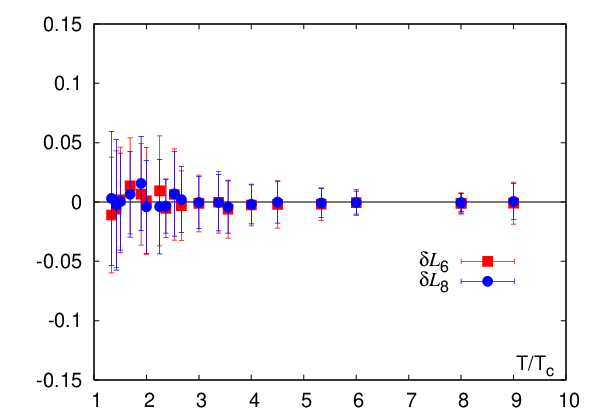
The results for the renormalized difference loops for and 8 are shown in Figure 9. They are consistent with zero at all temperatures. For the higher representations a statistically finer test is obtained with bare loops, since the errors on the renormalized loops are large. The results are shown in Figure 10. Even here, Casimir scaling is a good approximation, which gets better the higher the temperature.
IV.1 Two-flavor QCD

It is interesting to check whether Casimir scaling also holds for
QCD with quarks. Since dynamical
quarks break the center symmetry explicitly, and QCD has a
finite temperature cross over rather than a true phase transition,
the thermodynamic limit of the Polyakov loop below is non-vanishing.
In Figure 11 we show
for
at all temperatures, and
above . The latter representations are too noisy below
to add any information. These scaled quantities are almost independent of
down to . Below this
temperature we observe deviations to smaller values for the fundamental
representation, whereas the values for higher still coincide within errors.
Therefore we see a violation of Casimir scaling, between the fundamental
and other representations, when entering the
transition region which continues to the smallest temperatures analyzed.
These violations are relatively mild. Differences
between
for and remain statistically insignificant even at
the smallest temperatures, as shown in the
inset of Figure 11.
V The large- limit
The relation between Polyakov loops in different representations becomes rather simple in the limit of a large numbers of colors, Dumitru:2003hp. In this limit the expectation value of a Polyakov loop in representation can be expressed in powers of the fundamental () and anti-fundamental, () loop,
| (16) |
where the integers and are determined from the Young tableaux
of the representation . We investigate this large- factorization
using our data obtained for .
Following Dumitru:2003hp we analyze difference loops
| (17) | |||||
| (18) |
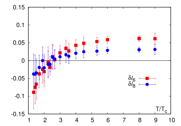
Naively, the correction terms are expected to be of the order of , i.e., about 33%. Results, shown in Figure 12 are clearly non-zero, except at around where all loops are one. Our results are comparable in magnitude to those in Dumitru:2003hp but show rather different temperature dependence. Below the corrections are relatively large, and the usefulness of the large- approximation seems doubtful. However, above this temperature, the difference loops are of order 5–10% of the loop itself, and therefore significantly smaller than the naive expectations. The large- approximation seems to fare better than expected. This is similar to the conclusion reached for the equation of state in Gavai:2004se.
VI Matrix Models
One could seek effective field theories for Polyakov loops in the form of matrix models, i.e., models in which each spatial site on the lattice, , contains a matrix valued “spin”, ,
| (19) |
and the integration measure is the Haar measure. For gauge groups the matrix takes values in SU(N). The action for these models can be written in the form
| (20) | |||||
where runs over every site in the lattice, over the nearest neighbors, is the Polyakov loop in the irreducible representation , i.e. the trace of the matrix, and is the triality of the irreducible representation . In this section we use the notation of Appendix A, i.e. traces are normalized to the dimension of the corresponding representation, . We also use the notation . The constraint of vanishing triality arises from the center-invariance of the pure gauge theory.
For SU(3), the effective action with only the leading term has been investigated extensively over the years. However, when adding all irreducible representations upto a certain , as varies, one needs the couplings
| (21) |
and so on.
A matrix model would be used to obtain the loop expectation values
| (22) |
where denotes the whole set of couplings in the action.
Equating these expressions to a sufficient number of observations
on , one would obtain the temperature
dependence of the couplings. Other predictions of matrix models,
which we do not explore here, are expectation values of moments (for
example, the Polyakov loop susceptibilities) and correlation functions
of loops.
Note an intrinsic complication in the matching procedure. Since
is scheme dependent,
the couplings that one extracts by any matching procedure must also
be scheme dependent. Note also that, in order to make contact with
a matrix model, one has to choose a renormalization scheme in which
. To the best of our knowledge, these
points have not been noted in the literature.


Furthermore, as the number of irreducible representations increases, the number of couplings
in the effective theory which need to be matched to data increases
rapidly. A determination of the effective action involves extraction
of the couplings through such matching at each temperature. This is an
ill-conditioned problem unless the series can be cut off, and the number
of couplings required is less than the number of pieces of data.
It is interesting to ask how one can bound the number of couplings needed
in the matrix model. If there are couplings to be determined,
then of the expectation values can be traded for the couplings,
and all other expectation values can be written in terms of these. For
example, for a one-coupling matrix model, , one could write
, for all . This
relation is RG invariant: in two different renormalization schemes, if
the values of at two different temperatures are the same,
then the values of will be equal, for each . For the pure
gauge theory the data in Figure 13 shows that the SU(3) pure
gauge theory requires a matrix model with only a single coupling. A single
coupling matrix model means that ratios such as
are fixed, and only one coupling is dependent on the temperature.
The temperature independent ratios of couplings define the shape of the
universal curves, ,
and the single tunable coupling says how the curve is traversed, in a
given renormalization scheme, as changes. Therefore, one can solve
the problem in two steps: first use the universal curves to fix the ratios
of the couplings, and finally solve the easier problem of finding the
single left over coupling. Since exact solutions for the loop expectation
values are not known for matrix models with , one has to either
solve the problem through a Monte Carlo simulation or in mean field theory.
Here we investigate the latter option.
Taking into account the irreducible representations and in the effective
action, one has
| (23) | |||||
where . Using this SU(3) relation, and making a mean-field approximation, we find that
| (24) | |||||
It is also possible to extend such a mean field treatment to models which include the octet representations. Using the invariance of the Haar measure, we can diagonalize the matrix, so that , and perform the integration over the remaining variables to give
| (25) | |||||
Putting all this together, we find
| (26) | |||||
In the mean-field theory the expectation values are computed simply as
| (27) |
where the can be expressed in terms of the angles and
using the formulae in eqs. (41-47) and the relation .
Some of the results are shown in Figure 13. The observed
Casimir scaling of loops implies a power-law dependence of loops on
each other. The matrix
model which includes only the coupling is
in fair agreement with the universal curve when
. However, it disagrees with the curve for
already when . By including terms in
and (in a fixed -independent ratio
to the curve for can be improved; but
this leads to no perceptible change in the curve for . However,
by introducing the coupling , and tuning the
-independent ratio , one can
contrive to improve the description of the two universal curves. However
the universal curves for etc., need further tuning.
The conclusion seems robust: the SU(3) pure gauge theory data can
be described within a single coupling matrix model. However, it seems
hard to construct a matrix model with a small number of terms which
reproduces the power-law dependence of on . The second
result has been obtained within a
mean field theory, and needs verification in a more complete approach,
such as the full simulation of such matrix models.
VII Adjoint sources and gluelumps
Polyakov loops in representations with non-zero triality vanish in the
confined phase of the pure gauge theory, since the Z(3) symmetry of
the action is realized on the states with large contribution to the
path integral. The behavior of loops with vanishing triality can be
different, because they are blind to the Z(3) symmetry involved in the
QCD phase transition. This study is confined to the octet loop since
all other triality zero loops that we constructed turned out to have
very large errors below .

A dynamical picture has been
advanced for the behavior of adjoint Polyakov loops below . An adjoint source can couple to a gluon in the medium to
form a colorless composite called a gluelump. Correlations of triality
zero loops can clearly be mediated by gluon exchange at any temperature,
leading to screening. Gluelumps provide a summary of the main features
of such screening Karsch:1998qj through two parameters: the free
energy of separated gluelumps determines the asymptotic value of an octet
Polyakov loop, the string breaking distance is the distance at which the
long-distance screening behavior sets in.
We found that the bare adjoint Polyakov loop below
assumes its thermodynamic limit, i.e., becomes independent of the volume
for lattices with . could
be renormalized using either the method for the octet loop
explained in Appendix B. However, we calculated
at more couplings than the adjoint correlator. Since we found that
agrees with (see Appendix B), we used the
given in Table 2 to obtain .
Table 3 lists the values found for the renormalized
adjoint Polyakov loop and Figure 14 compares
these results to those for the renormalized fundamental Polyakov loop,
. Although becomes rather small below , it is
clearly non-zero for all temperatures analyzed by us. We observe that
rises from at to just
below at . Crossing the critical temperature into
the deconfined phase, jumps almost an order of magnitude to
at . It is a little surprising to find the octet
loop, which is blind to the Z(3) symmetry, change discontinuously at the
symmetry-breaking transition. However, other triality-zero operators also
change discontinuously at the phase transition, most notably the energy
density.

We now address the issue of string breaking and determine the binding energy of the gluelump. The specific situation at , shown in Figure 15 serves as an example. We have shown , and, since it becomes too noisy at large distances, also the “color average” free energy , which has the same value at long distances. These free energies clearly show that adjoint sources are screened at large distances, in clear contrast to the linearly rising free energy, of sources in the fundamental representation. We calculate the free energy at infinite separation between the sources using the cluster property,
| (28) |
At zero temperature the energy stored in the field suffices to
put on-shell two gluons from the medium and form two disjoint
gluelumps Bali:2003jq. At finite temperature this
free energy can be identified with twice the gluelump screening mass.
Results for are collected in 3.
, is shown
in Figure 16 (upper panel).
It changes
little with , starting from GeV at and
subsequently falling to GeV just below .
At the lowest temperatures discussed here, indeed approaches
the value of GeV, which is twice the
mass of the gluelump obtained in Simonov:2000ky.
We define the string breaking distance by comparing
the Casimir scaled free energy with fundamental sources, ,
with the screened value of the free energy with adjoint sources,
| (29) |

| [GeV] | [fm] | ||
|---|---|---|---|
| – |
The results are collected in Table 3. In Figure 16 (lower panel) we show the resulting values of as a function of the temperature. There is rather mild change in with . It varies from fm at to fm just below . At the smallest temperature almost coincides with the value of fm Michael:1998sm.
VIII Conclusions
We examined the renormalized Polyakov loop in many different irreducible representations of the gauge group SU(3) in the thermodynamic limit of pure gauge QCD. It has been known for a long time that the ultraviolet divergences of the Polyakov loop can be absorbed into a multiplicative renormalization “constant” , where is the bare coupling. Such a renormalization factor does not depend on long distance physics, such as the temperature, (see eq. 7). We implemented such a renormalization procedure by explicitly constructing an iteration using only explicitly gauge invariant quantities starting from a reference temperature incorporating this idea (see Section III.2 for details). This so-called direct renormalization procedure was then used to extract the renormalized Polyakov loops in representations upto the 27 of SU(3) for a wide range of temperatures (see Section II).
The technical part of our paper also consists of extending the renormalization procedure of Kaczmarek:2002mc to Polyakov loops in arbitrary representations of the gauge group (see Appendix B). This is done by matching (gauge variant) correlation functions of sources in arbitrary representations to zero temperature values at the ultraviolet cutoff. Although one does not demand explicitly that the renormalization constant depends only on the bare coupling, the matching to zero temperature in the ultraviolet makes sure that this occurs. We checked that both renormalization procedures have the same, one real parameter, freedom of choice of scheme (see Appendix C). Having two drastically different renormalization schemes which are functionally equivalent allows us not only to use the most convenient scheme in any situation, but also to cross check the results by using both schemes whenever possible. This puts the results of the lattice measurements on very strong footing. Furthermore, the equivalence of the two procedures shows that the short distance as well as the large distance parts of the heavy quark free energies obtained in Coulomb gauge become gauge independent as proposed in Philipsen:2002az.
An interesting simplification occurs when Polyakov loop expectation values satisfy a relation called Casimir scaling (eq. 5). Then the renormalization factors in all the different representations essentially boil down to a single factor. Furthermore, large- factorization evolves from the large- limit of the quadratic Casimirs, and hence Casimir scaling could provide an alternative route to large- scaling. We have presented tests of Casimir scaling in Section IV and of direct large- factorization in Section V. Both turn out to be reasonably reliable away from . However, Casimir scaling is significantly more reliable and may provide a good route to scale large- predictions down to .
One subject of abiding interest is whether the high temperature phase of QCD can be described by a matrix model. We test this question in Section VI. Casimir scaling implies that there are universal (renormalization scheme independent) relations between the renormalized Polyakov loop expectation values such that all the loops we studied depend only on the value of the fundamental loop. This implies that a matrix model description could work well away from . A single parameter variation of all couplings in the model would then reproduce the data on Polyakov loops, the temperature dependence of the couplings being, of course, renormalization scheme dependent. However, it seems that a simple model with a small number of parameters is not able to reproduce the power-laws in the lattice data, at least within the mean-field analysis of the matrix model performed here.
Due to the Z(3)-symmetry of the pure gauge theory, all Polyakov loops with non-zero triality vanish in the confined phase of the pure gauge theory. For the adjoint representation we have observed small, but non-zero, values below for the first time in the thermodynamic limit (see Section VII). Since static adjoint sources can form bound states, called gluelumps, with dynamical gluons, correlations of adjoint loops show screening (string breaking) even in the confined phase. As a result, heavy quark free energies have a finite asymptotic value while for zero-zero triality they rise linearly with distance. Some aspects of the free energy can be captured into the phenomenology of gluelumps through a mass and radius parameter. We present results for these quantities.
Our primary technical result is the systematic development of two parallel renormalization procedures for Polyakov loops in arbitrary representations of the gauge group. This allows us to check that Casimir scaling of the renormalized loops is satisfied to good accuracy away from . This is our main physical result, since it leads on to the discussion of large- factorization and the matrix model description of lattice data.
Acknowledgment
We wish to thank J. Engels, F. Karsch, R. D. Pisarski, Y. Schröder and F. Zantow for fruitful discussions. This work has partly been supported by contract DE-AC02-98CH10886 with the U. S. Department of Energy. At an early stage of this work K. H. has been supported by the DFG under grant GRK 881/1. S. G. would like to acknowledge the hospitality of the University of Bielefeld.
References
- (1) http://www.claymath.org/millennium/Yang-Mills_Theory.
- (2) G. ’t Hooft, Nucl. Phys. B72, 461 (1974).
- (3) G. Policastro, D. T. Son, and A. O. Starinets, Phys. Rev. Lett. 87, 081601 (2001), hep-th/0104066.
- (4) B. Bringoltz and M. Teper, Phys. Lett. B645, 383 (2007), hep-th/0611286.
- (5) B. Lucini, M. Teper, and U. Wenger, JHEP 01, 061 (2004), hep-lat/0307017.
- (6) R. V. Gavai, S. Gupta, and S. Mukherjee, Phys. Rev. D71, 074013 (2005), hep-lat/0412036.
- (7) R. D. Pisarski, Phys. Rev. D74, 121703 (2006), hep-ph/0608242.
- (8) A. Dumitru, Y. Hatta, J. Lenaghan, K. Orginos, and R. D. Pisarski, Phys. Rev. D70, 034511 (2004), hep-th/0311223.
- (9) A. Dumitru, J. Lenaghan, and R. D. Pisarski, Phys. Rev. D71, 074004 (2005), hep-ph/0410294.
- (10) A. Dumitru, R. D. Pisarski, and D. Zschiesche, Phys. Rev. D72, 065008 (2005), hep-ph/0505256.
- (11) A. Dumitru, D. Roder, and J. Ruppert, Phys. Rev. D70, 074001 (2004), hep-ph/0311119.
- (12) E. Megias, E. Ruiz Arriola, and L. L. Salcedo, JHEP 01, 073 (2006), hep-ph/0505215.
- (13) E. Megias, E. Ruiz Arriola, and L. L. Salcedo, Phys. Rev. D74, 065005 (2006), hep-ph/0412308.
- (14) C. Ratti, M. A. Thaler, and W. Weise, Phys. Rev. D73, 014019 (2006), hep-ph/0506234.
- (15) P. N. Meisinger, M. C. Ogilvie, and T. R. Miller, Phys. Lett. B585, 149 (2004), hep-ph/0312272.
- (16) K. Fukushima, Phys. Rev. D68, 045004 (2003), hep-ph/0303225.
- (17) D. Diakonov and M. Oswald, Phys. Rev. D70, 105016 (2004), hep-ph/0403108.
- (18) B.-J. Schaefer, J. M. Pawlowski, and J. Wambach, (2007), arXiv:0704.3234 [hep-ph].
- (19) D. Blaschke, M. Buballa, A. E. Radzhabov, and M. K. Volkov, (2007), arXiv:0705.0384 [hep-ph].
- (20) S. Ghosh et al., arXiv:0710.2790 [hep-ph].
- (21) K. Kashiwa, H. Kouno, M. Matsuzaki, and M. Yahiro, (2007), arXiv:0710.2180 [hep-ph].
- (22) O. Kaczmarek, F. Karsch, P. Petreczky, and F. Zantow, Phys. Lett. B543, 41 (2002), hep-lat/0207002.
- (23) P. Weisz, Nucl. Phys. B212, 1 (1983).
- (24) P. Weisz and R. Wohlert, Nucl. Phys. B236, 397 (1984).
- (25) B. Beinlich, F. Karsch, E. Laermann, and A. Peikert, Eur. Phys. J. C6, 133 (1999), hep-lat/9707023.
- (26) B. Beinlich, F. Karsch, and A. Peikert, Phys. Lett. B390, 268 (1997), hep-lat/9608141.
- (27) C. R. Allton et al., Phys. Rev. D66, 074507 (2002), hep-lat/0204010.
- (28) C. R. Allton et al., Phys. Rev. D68, 014507 (2003), hep-lat/0305007.
- (29) A. M. Polyakov, Nucl. Phys. B164, 171 (1980).
- (30) V. S. Dotsenko and S. N. Vergeles, Nucl. Phys. B169, 527 (1980).
- (31) G. P. Korchemsky and A. V. Radyushkin, Nucl. Phys. B283, 342 (1987).
- (32) M. Creutz, Phys. Rev. D23, 1815 (1981).
- (33) E. Gava and R. Jengo, Phys. Lett. B105, 285 (1981).
- (34) G. S. Bali and K. Schilling, Phys. Rev. D47, 661 (1993).
- (35) F. Karsch, E. Laermann, and A. Peikert, Phys. Lett. B478, 447 (2000).
- (36) S. Gupta, Phys. Rev. D64, 034507 (2001), hep-lat/0010011.
- (37) O. Kaczmarek, F. Karsch, E. Laermann, and M. Lütgemeier, Phys. Rev. D62, 034021 (2000), hep-lat/9908010.
- (38) S. Datta and S. Gupta, Phys. Rev. D67, 054503 (2003), hep-lat/0208001.
- (39) U. M. Heller and F. Karsch, Nucl. Phys. B251, 254 (1985).
- (40) Y. Schröder, Phys. Lett. B447, 321 (1999), hep-ph/9812205.
- (41) G. S. Bali and P. Boyle, (2002), hep-lat/0210033.
- (42) P. H. Damgaard, Phys. Lett. B194, 107 (1987).
- (43) G. S. Bali, Phys. Rev. D62, 114503 (2000), hep-lat/0006022.
- (44) V. I. Shevchenko and Y. A. Simonov, Phys. Rev. Lett. 85, 1811 (2000), hep-ph/0001299.
- (45) F. Karsch and M. Lütgemeier, Nucl. Phys. B550, 449 (1999), hep-lat/9812023.
- (46) G. S. Bali and A. Pineda, Phys. Rev. D69, 094001 (2004), hep-ph/0310130.
- (47) Y. A. Simonov, Nucl. Phys. B592, 350 (2001), hep-ph/0003114.
- (48) C. Michael, (1998), hep-ph/9809211.
- (49) O. Philipsen, Phys. Lett. B535, 138 (2002), hep-lat/0203018.
- (50) O. Jahn and O. Philipsen, Phys. Rev. D70, 074504 (2004), hep-lat/0407042.
- (51) S. Necco and R. Sommer, Nucl. Phys. B622, 328 (2002), hep-lat/0108008.
Appendix A Polyakov loops in irreducible representations of SU(3)
In order to obtain Polyakov loops in higher irreducible representations of SU(3) than the fundamental, we may use the theorem that the character in a direct product representation is the product of the corresponding characters, . Then the direct product can be reduced using the Clebsh-Gordan series to yield the Polyakov loop in various representations.
We use the following identities:
| (30) | |||||
| (31) | |||||
| (32) | |||||
| (33) | |||||
| (34) | |||||
| (35) | |||||
| (36) | |||||
| (37) | |||||
| (38) |
where we have specified the irreducible representations both in terms of its dimension
and through the canonical label where and are
integers. Recall that the maximum weight in irreducible representation is , and the dimension of this irreducible representation is
. The notation stands for the
irreducible representation , and denotes the irreducible representation . Note
that interchanging and gives the complex conjugate irreducible representation. The triality of
an irreducible representation can be defined to be . In each expression above,
the trialities of all the irreducible representations on the right must be equal, and must equal
the sum of the trialities (mod 3) of the irreducible representations on the left. This can be
used as a check.
More concretely, take the product over links and the trace defining the
Polyakov loop in the of SU(3),
| (39) |
where is a complex number. Here the trace is normalized such that the unit matrix traces to 3. The Polyakov loop in an irreducible representation is the character in that irreducible representation. Hence, given the loop in one irreducible representation, that in the complex conjugate irreducible representation is obtained by complex conjugation. One specific example is
| (40) |
where is the complex conjugate of . The Polyakov loop in the trivial irreducible representation is unity (which gives vanishing potential in this irreducible representation). Next we construct the series of other Polyakov loops,
| (41) | |||||
| (42) | |||||
| (43) | |||||
| (44) | |||||
| (45) | |||||
| (46) | |||||
| (47) |
Further irreducible representations can be obtained if needed. Two of the reductions for the direct product have not been used. The Polyakov loop values in normalization used elsewhere in this paper is obtained by writing .
| 1 | |||||
| 2 | |||||
| 2 | |||||
| 0 | |||||
| 0 | |||||
| 1 | |||||
| 1 | |||||
| 2 | |||||
| 0 |


Appendix B renormalization
The renormalization procedure Kaczmarek:2002mc can be extended to static sources in arbitrary representations of the color group. For simplicity we will only discuss adjoint sources here in detail, but the generalization to other representations is straight forward.
Given an SU(3) matrix in the fundamental representation, , the corresponding adjoint matrix, , is
| (48) |
where are the Gell-Mann matrices. From the hermiticity of and cyclicity of the trace all matrix elements are real. This formula can be used to convert all link elements from the fundamental to the adjoint.
The thermal Wilson line in the adjoint representation is
| (49) |
Another way to define it is to take the fundamental Wilson line of eq. (1) and convert it to the adjoint using the prescription of eq. (48). The adjoint Polyakov loop is the trace
| (50) |
As before, we have normalized the trace such that the trace of the unit matrix is 1.
Define the correlator of two adjoint thermal Wilson lines,
| (51) |
and . This correlator is clearly gauge dependent, and hence we define it through Coulomb gauge fixing (see Philipsen:2002az; Jahn:2004qr for more on this point). The free energy with two static adjoint sources a distance apart is
| (52) |
Here and denote bare correlators and free energies; the same notation without a tilde will denote renormalized quantities.
Since the Polyakov loop is renormalized multiplicatively, the free energies are additively renormalizable. We match the finite temperature free energy to the zero temperature potential at the smallest attainable distance, , on a lattice
| (53) |
where is the zero temperature potential in the fundamental representation. We use the potential derived in Necco:2001xg. In the matching procedure we have used Casimir scaling of the potential at short distances. This is seen in continuum Schroder:1998vy and lattice Bali:2002wf perturbation theory. In Figure 17 we show the renormalized quark-antiquark free energies for static sources in the adjoint () and fundamental () representations together with the Casimir scaled zero temperature potential . The data clearly validates the assumption of short distance Casimir scaling on which the procedure rests.
Once the free energies have been renormalized at small distances, their large distance behavior is fixed. The asymptotic value can be used to the define the renormalized Polyakov loop through the cluster property
| (54) | |||||
This completes the renormalization procedure for the octet loop. The requirement that depend only on is not explicitly imposed in the renormalization procedure. However, the results, plotted in Figure 18 show that this is obtained. The figure also shows that Casimir scaling of the renormalized Polyakov loop is obtained, since and agree.
Any unitary matrix with unit determinant is uniquely specified by eight real numbers, which are coordinates in the abstract group SU(3). Given these coordinates, there are canonical techniques for building matrices in any representation which generalize eq. (48). Hence, given the thermal Wilson line in the fundamental, one can construct the equivalent for arbitrary . From that one can generalize every step of the procedure from eq. (51) on for any .
Appendix C Renormalization schemes

In the direct renormalization procedure the freedom of scheme choice is the multiplicative ambiguity , for some constant . This implies that at another temperature the renormalized Polyakov loop is scaled by the factor . In the renormalization procedure it is the freedom of defining the zero of the potential
| (55) |
Using Casimir scaling for the short distance potential, this clearly leads to the scaling
| (56) |
which incorporates Casimir scaling for the Polyakov loop. Our standard scheme choice corresponds to choosing such that the triplet potential at is given by the results of Necco:2001xg.
Appendix D Color average free energies


We now turn to color averaged -free energies. Since the corresponding correlators can be obtained without a costly gauge fixing, we were able to calculate for representations in the temperature range on lattices. The color average correlator for at temperature in representation is defined by
| (57) |
where the star denotes complex conjugation. The color average free energy . If Casimir scaling holds, then
| (58) |
We test this relation below and above .
Below we employ the renormalized average free energies
| (59) |
for the three lowest temperatures divided by their Casimir in fig. 20. The renormalization constants used are those found by the renormalization procedure described in sec. III.3. Thus for the smallest distances all curves coincide as a consequence of the renormalization procedure. However, for all and representations deviations to smaller values start to show up quite early, i. e. for separations for and for , respectively. This effect is more pronounced for the adjoint average free energy than for the sextet. The effect of string breaking sets in at larger distances than shown here and will be discussed in sec. VII.
Above we compare
| (60) |
divided by their Casimir for the same representations in fig. 21. We observe screening to take place in both higher representations. The curves for both and deviate to smaller values compared to the fundamental case. We find that the ordering
| (61) |
holds throughout the entire distance interval above .
Thus, we conclude, that Casimir scaling (58) is clearly violated for the average free energies in the temperature range for the fundamental, sextet and adjoint representations.