The Ly Emission Line as
a Cosmological Tool
Abstract
NEC FASCES
NEC OPES
SOLA ARTIS
SCEPTRA PERENNANT
Not power, not wealth,
only the reign
of art and science
shall persist
Tycho Brahe 1546 - 1601
This thesis deals with different aspects of a special kind of high redshift galaxy, namely Ly emitters. Ly emitters are galaxies found through their Ly emission, at redshifts larger than where the emission line has been redshifted into the optical or near-infrared regime. The thesis has two main parts; a lower redshift, observational part () and a more technical/theoretical very high redshift part ().
In the first, lower redshift part I present the analysis of a narrow-band image taken in the GOODS-S field, focused on a redshift for Ly of . The image, covering a central part of the GOODS-S field revealed 25 Ly emitting candidates, of which one turned out to be a so-called Ly “blob”. Ly blobs are large nebulae of gas emitting a large amount of light in the Ly line. They can be very bright ( erg s-1) and have projected diameters as large as 150 kpc. Three possible mechanisms have been proposed to explain this phenomenon; i) star formation and “super-winds”, ii) AGN activity and iii) cold accretion. The blob in GOODS-S turned out to be the first Ly blob best explained by cold accretion, and was published in a Letter to the Editor in A&A in June 2006 (Nilsson et al. 2006a). The remaining 24 Ly emitters were analysed together, in order to gain insight in the nature of galaxies selected through narrow-band imaging for redshifted Ly emission. An extensive SED fitting was performed and the results also included the discovery of an apparent filamentary structure and a comparison to Lyman-Break Galaxies at similar redshifts. The results from this analysis is accepted for publication in A&A in Nilsson et al. (2007).
In the second part, I discuss future, very high redshift narrow-band surveys for Ly emitters. In February 2005, the idea of buying a narrow-band filter for the, then half way through its construction, Visible and Infrared Survey Telescope for Astronomy (VISTA) to search for Ly emitters at very high redshift started. In Chapter 4 I describe the science case for the filters and the process of designing and procurement of the filters. In this chapter is also described how the initial idea for a narrow-band survey was developed into what has become ELVIS - Emission Line galaxies with VISTA Survey, part of the Ultra-VISTA survey which will – hopefully – start observing in the Spring of 2008. The need for better predictions of what may be observed with this type of survey was realised early on, and in Chapter 5 I present a paper in which we try to make more accurate predictions of the outcome of very high redshift narrow-band surveys for Ly emitters using two theoretical models.
Finally, in a project unrelated to the other two parts of the thesis, I present a search for a “Fundamental plane” of Ly emitters in the colour space produced by large-scale multi-wavelength surveys such as GOODS or COSMOS. The goal of the project was to decide the most efficient narrow-band colour selection method for detecting Ly emitters at several different redshifts. We also wanted to optimise the selection method to exclude interloper galaxies such as lower redshift [OII]-emitters. In this thesis I present the results of this study.
Acknowledgments
I am tremendously grateful to all who have in some way helped or supported me and my work that has lead to this thesis. I would like to thank IDA, DARK and ESO for funding my PhD studentship and for taking me in. I have been helped by many people. In particular my two supervisors Johan Fynbo and Palle Møller have been pillars of support. We may not always have agreed, but I have learned incredibly much from both of you and I feel very fortunate in my supervision. I am not sure that ELVIS would have happened if Johan had not believed in my crazy idea. Along the same line, I should probably thank my room-mate at that winter school in Obergurgl in February 2005 for giving me encouraging words when I woke her up in the middle of the night to tell her about my idea. I am sorry I do not remember her name! I am also very grateful for help with the VISTA project from Will Sutherland, who has been a great help and support and who always answered my e-mails with questions very quickly. Further input and help with ELVIS has been thankfully received from Wolfram Freudling, Michelle Doherty, Lisbeth Fogh-Grove, Piero Rosati, Ian Smail, Jim Emerson, Jean-Gabriel Cuby and Gavin Dalton.
Another person that has been very important to me socially and professionally is my fiancee Ole Möller. I met Ole shortly after moving to Munich and it was interest at first sight. Our personal relationship has since then evolved into a professional dito, when we realised that Oles love for programming filled a void in my own skills. I am thus grateful and proud of the fruitful joint ventures we have had so far in writing a beautiful SED fitting code and a “fundamental plane” code. Ole, you have also been an amazing support when listening to my rants during both ups and downs in my life. Thank you.
Further, I would like to thank Alvaro Orsi, Matthew Hayes and Christian Tapken for interesting meetings and discussions which have led to more or less completed projects. I would like to thank all my other co-authors for wanting to work with me and for your assistance in producing brilliant results! Thank you Árdís and José María for reading and commenting on my thesis manuscript and for being good friends throughout my PhD time. A special thanks to Klaus Meisenheimer and Hans-Walter Rix at Max-Planck-Institut für Astronomie in Heidelberg for believing in me to the extent that you hired me for a post-doc seven months before I was due to finish my PhD. I look forward to working with you. Of course I also want to thank my thesis committee — Sangheeta Malhotra, Göran Östlin and Jens Hjorth — for taking time to evaluate my work.
Finally, a thanks to all my friends at ESO and DARK, who made the work-days more pleasant, and to my mother Yvonne for loving support and my cat Matrise for unconditional love irrespective of my mood. To the people that have helped me: you are my heroes. Thank you all.
Chapter 1 Introduction
1.1 The high redshift Universe
1.1.1 Brief history of our Universe and the redshift
Our Universe was created in the Big Bang. In the first few fractions of a second the Universe was extremely hot, but it expanded and cooled rapidly. After this initial stage of “primeval soup”, where particles and radiation were coupled and high energy physics governed everything, a period of cooling began. At around yrs after the Big Bang, the Universe had cooled and de-pressurised enough so that nuclei had formed and the electrons had been captured to make neutral atoms. This is called recombination, see Fig. 1.1. At this time, the photons created in the Big Bang and immediately thereafter were released and could begin their journey through the Universe. This radiation is called the Cosmic Microwave Background (CMB) and is an almost perfect blackbody emission with a peak temperature of 2.73 K. The irregularities seen in the CMB indicate that there were slight inhomogeneities in the matter density at recombination. These inhomogeneities later turned into the structures we see today.
After recombination, these peaks in the matter-density distribution continued to contract due to gravity and after some Myrs, the first stars were born. These were massive stars that burned their fuel quickly, exploded and enriched their surroundings. Soon, more stars were forming and galaxies started to take shape. Also, the first quasars may have lit up at this time. These galaxies and quasars produced a large amount of UV radiation and this radiation field ensured that the Universe would once again become ionised and the electrons separated from the atoms. This is called the re-ionisation and is believed to have occurred at , between Gyrs after the Big Bang. The search for when exactly this happened is a hot topic today, as our telescopes push further and further back in time. The current record in redshift for an observed galaxy today is (Iye et al. 2006), and observations in the near future should be able to push this record to redshifts around , see also Chapter 4 and 5.
From redshift and on, the Universe has continued to expand, cool, gather mass in clusters and galaxies and produce stars. The redshift at which the star formation rate per volume peaked appears to be around redshift , see Fig. 1.2. Our Sun was formed some 4 Gyrs ago, corresponding to redshift .
So, what is redshift? Redshift occurs as photons travel through the Universe, which simultaneously expands. An analogy is the change in pitch when a trains whistle or an ambulances sirens pass your ear. The sound waves are compressed in front of the train, thus the pitch goes up, and elongated behind the train, thus the decrease in pitch again. In space, the size of the Universe changes with time according to the scale factor a(t). Thus, photons travelling towards us will stretch its wavelength due to the expanding Universe and the light will be shifted towards the red, i.e. redshift. Redshift is defined as:
| (1.1) |


1.1.2 Methods of finding high redshift galaxies
In our constant search for knowledge we want to understand how the stars and galaxies were formed, and how they evolved. We can make models of star formation, but ultimately we need observations of the young Universe. Thus, we search for high redshift galaxies, whose light was emitted a long time ago, corresponding to in Eq. 1.1. That means that the light we observe from a galaxy at redshift was emitted from a very young galaxy, when the Universe was only Gyrs old. Looking further away in redshift means looking further into our past. And thus finding a large, representative sample of galaxies at different redshifts will give us insight into galaxy formation and evolution.
There are many methods of finding star forming galaxies in the high redshift Universe, and each method explores different classes of galaxies. One of the major questions in observational cosmology is thus what are the relations between these classes. This thesis explores properties of high redshift galaxies selected by their Ly emission (see below). In this introduction I discuss several different methods used to detect high redshift galaxies.
Lyman Break Galaxies selection
One of the most common methods in the last decade, now comprising an impressive catalogue of thousands of galaxies, has been the selection based on photometric redshifts gained from observations of the “Lyman Break” in galaxies. The Lyman Break, located at 912 Å in the spectrum of a galaxy, represents the cut-off energy where the single electron of a hydrogen atom is ionised. Almost all the UV light of a galaxy is absorbed at wavelengths shorter than this, as hydrogen is extremely abundant in galaxies. Thus, a “break” in the spectrum of the galaxy. The Lyman Break Galaxy (LBG) selection method was pioneered by Steidel et al. (1996; 1999; 2000; 2003), but has also been used by many other groups (e.g. Madau et al. 1996; Pettini et al. 2001; Bunker et al. 2004; Stanway et al. 2004; Ouchi et al. 2004a,b; Wadadekar et al. 2006). An illustration of the method is found in Fig. 1.3. As can be seen, a galaxy will appear to “drop out” in the bluest filter, hence the method is sometimes also referred to as the drop-out technique. Spectroscopic follow-up is necessary to confirm the high redshift nature of the galaxy.
The Lyman Break technique can be used for a wide range of redshifts, when different filters are used for the selection. Table 1.1 gives the filters and redshifts commonly used, or proposed to be used.
| Blue filter | Red filters | Redshift range | |
|---|---|---|---|
| U | B, G, R, V | 2.5 - 3.5 | |
| B | G, R, V | 3.5 - 4.5 | |
| V | i, z | 4.5 - 6.0 | |
| i | z, J | 6.0 - 7.5 | |
| z | J, H, Ks | 7.5 - 11.5 | |
| J | H, Ks | 11.5 - 15.5 |
The technique is typically spectroscopically complete to an R band magnitude of for U-band drop-outs but the rate of confirmation falls for higher redshift LBG candidates (Giavalisco 2002). A few studies of the properties of LBGs such as masses, dust content, ages etc. have been made so far. These studies are well summarised in Giavalisco (2002). LBGs appear to have ages ranging from a few to several hundred Myrs or even up to 1 Gyr. Stellar masses lie in the range . Papovich, Dickinson & Ferguson (2001) find very high extinction in their sample of LBGs, with , while Shapley et al. (2001) and Verma et al. (2007) find more modest values of in their samples. Thus, it appears that LBGs are medium mass and medium dusty galaxies, with high star formation rates of several hundred solar masses per year (Shapley et al. 2001). Several groups have also detected clustering in LBGs, similar to that of Ly emitters (Steidel et al. 1998; Giavalisco et al. 1998; Ouchi et al. 2004b; see also sec. 1.3.5).
Damped Ly Absorption selection
When observing a quasar at high redshift, sometimes a gas cloud with a high column density will be found along the same line of sight. This is not as uncommon as one might think. When a cloud with an HI column density larger than cm-2 is observed along the sight-line of a quasar it is called a Damped Ly Absorber (DLA) as its Ly absorption line will be damped. Thus, the DLA technique is based on finding high column density galaxies by searching for absorption lines in the spectra of quasars. An illustration of the method can be found in Fig. 1.4.

The search for DLA systems began already in the mid-80s but a large sample of DLA galaxies were not collected until ten years ago (for a review, see Wolfe, Gawiser & Prochaska 2005).
A problem with this selection method is the apparent proximity of the quasar in the sky, making imaging follow-up difficult. However, DLA system can still give valuables insights into properties such as the neutral gas fraction in the Universe, chemical evolution and metallicity production across a large redshift range and gas kinematics in galaxies.
Selection based on sub-millimeter emission
The Spectral Energy Distribution (SED) of a dusty starburst galaxy will have its peak emission at wavelengths of mm, see Fig. 1.5. These galaxies will, however, not have significant emission in the optical or near-infrared parts of the spectrum. Thus, observing the sky in the sub-mm will reveal a class of galaxies otherwise left unstudied. Due to the difficulties in building detectors for these wavelengths, it was not until the commissioning of the SCUBA detector (Holland et al. 1999) on the James Clerk Maxwell Telescope (JCMT) in 1997 that progress was made in this field of study.

As the sample of sub-mm selected galaxies has grown to be (e.g. Blain et al. 2002; Ivison et al. 2005), the median redshift of this sample appears to be , although sub-mm emission should in theory be just as efficient to detect galaxies between .
Two, related, problems with selecting galaxies based on sub-mm emission are that the beam sizes are still very large (of the order 10 arcsec) and that identification of optical/infrared counterparts are difficult. The process of identifying a counterpart is generally done by first searching for a radio counterpart, since radio observations have smaller beam sizes and radio emissions have been shown to be proportional to sub-mm emission (e.g. Carilli & Yun, 1999). Following identification of a radio counterpart, an optical or infrared counterpart may be found. However, even with radio identifications, optical/infrared identifications can be difficult to make. The sample of galaxies with confirmed counterparts display a wide variety of properties including AGN and starburst activity, as well as signs of recent mergers (Ivison et al. 2000; Blain et al. 2002). Future instruments such as SCUBA-II and ALMA will hopefully give us a better insight into the nature of sub-mm selected galaxies.
Gamma Ray Burst selection
Gamma Ray Bursts (GRBs) are violent explosions, more energetic than supernovae. The name derives from the fact that GRBs are found through a burst of gamma ray emission. GRBs are typically divided into two classes of events, long or short duration bursts; where the long bursts are believed to be related to relativistically beamed extreme versions of (hundreds of times brighter than) supernovae (e.g. Hjorth et al. 2003), i.e. the death throws of a massive star, and the short bursts are believed to occur when two compact objects (i.e. neutron stars or black holes) collide (e.g. Hjorth et al. 2005). The method of finding high redshift galaxies using GRBs is to use the location of the GRB to search for its host galaxy. The gamma ray event of the GRB triggers a satellite based telescope, such as for instance the Swift11 1 http://www.swift.psu.edu/ telescope, to slew to the part of the sky where the event occurred. In general, the accuracy of the positioning from the gamma ray telescope is poor, e.g. of the order of arcminutes, and it is followed up with an X-ray telescope, as X-rays are easier to pin-point and most GRB afterglows emit strongly also in X-rays. When the location of the GRB has been localised to a smaller error box, optical/near-IR telescopes take over and search for the optical/near-IR afterglow of the GRB. Thus, the GRB can finally be completely localised, to subarcsecond resolution, using an optical detection. After the GRB has faded, this position can be observed to greater depth to search for the host galaxy of the GRB. Host galaxies of GRBs are often blue, star-forming galaxies (e.g. Bloom et al. 1998; Sokolov et al. 2001; Gorosabel et al. 2005; Fruchter et al. 2006).
Ly selection
A very efficient method to detect high redshift galaxies is to observe the sky with a narrow-band filter focused on the Ly emission line at a particular redshift. A narrow-band filter is a filter that allows only a very small range of wavelengths to pass through it and blocks all other light. This will result in a narrow range of redshifts for Ly, typically . In order to find the Ly emitters, the same field is then observed with one or two broad band filters with the same, or near the same, central wavelength as the narrow-band filter. The broad band observations then probe the continuum of the source and emission-line galaxies are found by comparing the narrow-band flux with the broad band flux. Objects with a high flux ratio of narrow-band vs. broad band measurement are selected.
In the work that is presented in this thesis, the equivalent width of the line has been calculated in the selection process. Equivalent width (EW) is a measure of the strength of an emission- (or absorption-) line and is defined as
| (1.2) |
where is the flux in the emission/absorption line and is the flux density in the continuum at the central wavelength of the line. The EW is positive for emission lines and negative for absorption lines. Object with a flat continuum, without emission or absorption lines, should have an EW of zero. The method used to find Ly emitters in our surveys is described in more detail in section 3.3.2. In sec. 1.3, results from past surveys for Ly emitters are reviewed.
1.2 Ly in a historical perspective
This thesis deals with high redshift galaxies found through their Ly emission lines. The Lyman series (Ly, Ly, Ly…) are the emission lines created when an electron falls from any higher energy level, back to the ground state of the simplest and most abundant atom in the Universe, the Hydrogen atom. The strongest line, with longest wavelength (1215.67 Å), is the one from the second energy level to the first; Ly. The Lyman series are named after Theodore Lyman, a physicist who discovered them during the first two decades of the 20th century.
In the mid 1920s, Menzel (1926) and Zanstra (1927) each separately discussed the ionisation of emission lines in planetary nebulae, including Ly, and in 1945 Chandrasekhar discussed the radiative equilibrium of Ly. The first observations of highly redshifted Ly came with the discovery of quasars, or QSOs. It was in the 1950s that star-like objects were found unexpectedly to have bright radio emission. In 1963 Schmidt published the first “large redshift object” (3C 273) and just two years later a quasar was identified to be at redshift 2.01 through its Ly emission (3C 9; Schmidt 1965). It was at the same time as these observations were published that theoretical predictions for Ly emission and absorption in the young Universe started. Gunn & Peterson (1965) observed that the continuum of the quasar on the blue side of the Ly emission line was not absorbed and put an upper limit on the absorption by neutral hydrogen clouds in the line of sight towards the quasar. Bahcall (1966) predicted the line strengths of the Lyman lines, and finally Partridge & Peebles (1967) published the first article with predictions on the observability of the Ly from young star forming galaxies, not QSOs, at high redshifts. Their results have a remarkable level of agreement with the results of present day Ly surveys and sparked the field of narrow-band surveys for Ly emitters.
It would, however, take a bit more than two decades before the first high redshift Ly emitters were to be found. Immediately following the Partridge & Peebles (1967) paper, some groups attempted to discover these “primeval galaxies” (Partridge 1974; Davis & Wilkinson 1974; Meier 1976; Hogan & Rees 1979) but they were all unsuccessful. The narrow-band technique (see sec. 1.1.2) was brought into use in the late 1980s but the first surveys were unsuccessful (e.g. Pritchet & Hartwick 1989, 1990; Rhee, Webb & Katgert 1989). The first detections came in the early 1990s by Lowenthal et al. (1991), Wolfe et al. (1992), Møller & Warren (1993) and Macchetto et al. (1993). From there on, narrow-band surveys became more and more frequent and successful. Examples are the LALA survey (Rhoads et al. 2003; Dawson et al. 2003), the Building the Bridge Survey (Fynbo et al. 2003) and the studies in the fields of radio galaxies (Venemans et al. 2007). To the publication date of this thesis, more than 550 Ly emitters have spectroscopic confirmation with redshifts ranging from , see Fig. 1.6.
1.3 What are Ly emitters?
1.3.1 Objects that emit Ly
A multitude of objects in the Universe emit Ly. To ionise the hydrogen atom, a photon with a wavelength shorter than 912 Å is needed. This kind of UV radiation can come from several different sources. The most common sources are young, massive and short-lived stars of the spectral type O and B. The more massive the star, the shorter it lives and the bluer its spectrum is. O and B stars are the most massive ones known in the Universe, hence they emit almost all of their light in the UV range of the spectrum. They are also very luminous because they are so massive. Hence, Ly is often seen emitted from regions with intense star formation, because the short lifetime of the O and B stars make them burn out and die before they have time to move away from their birthplace. So, O and B stars and hence star forming galaxies are often intense sources of Ly.
Another type of object that often emits Ly, or has a Ly halo around it, are quasars and active galactic nuclei (AGN, Schmidt 1965; McCarthy 1993; Villar-Martín et al. 2005). These objects are believed to consist of massive black holes accreting material from accretion disks surrounding them. The fact that AGNs have an accretion disk is in part crucial for the large Ly haloes seen around this type of object, as the outcoming UV light is highly collimated along the axis of the disk (Weidinger et al. 2005). That radio jets are observed in some AGN is also one of the primary arguments of why there should be an accretion disk (Urry & Padovani 1995). The spectrum emitted by an AGN has three components, an X-ray power law spectrum, an infrared bump and a strong UV continuum emission component (Collin 2001). It is this UV component that ionises the hydrogen, which will then emit Ly in two highly ionised cones perpendicular to the disk (Haiman & Rees 2001; Weidinger et al. 2005). Hence, AGN are also Ly emitters.
A third possibility for the production of Ly photons is the theory of “cold accretion” (e.g. Fardal et al. 2001; Dijkstra et al. 2006a,b; Nilsson et al. 2006a). The general idea is that if the Universe contains dark matter haloes that initially have no galaxy in them but plenty of neutral hydrogen gas, then the gas would slowly start to fall in, onto the halo because of the gravitational potential energy. This would cause the material to heat up because of the loss of potential, and this heat could theoretically be cooled off by emitting Ly photons. The idea was prompted after a similar effect had been seen in clusters of galaxies were the gas fell in, heated up and cooled via X-ray emission (Fabian 1994). On a galaxy size scale, this emission could be predominantly in Ly. Until recently this had never been observed. However, as can be read in Chapter 2, we have published the first paper presenting a probable observation of this phenomenon.
1.3.2 Redshift distribution of Ly emitters
Ly can be observed with ease in the optical regime, covering approximately the redshift range of . At even higher redshifts, observations are possible in the near-infrared. The distribution of spectroscopically confirmed Ly-emitters at the time of writing this thesis can be found in Fig. 1.622 2 I have been trying to keep an up-to-date list of all spectroscopically confirmed Ly emitters. The true number may be slightly higher if I missed a publication. It will not be lower..

A much larger sample of candidate Ly-emitters exist, with photometric selection only. Spectroscopic follow-up generally has a success rate of 75 - 90% for surveys (Fynbo et al. 2001; 2003), and approximately 50 - 75% for surveys (Taniguchi et al. 2005; Kashikawa et al. 2006; Shimasaku et al. 2006).
The multiply peaked distribution shown in Fig. 1.6 can be explained in the following way. The peak at redshift is most likely due to the CCD being most sensitive at around 5000 Å as well as to the abundance of [OIII] emission targeted narrow-band filters at most ground-based observatories. The peak at is due to the LALA survey (Rhoads et al. 2000; Dawson et al. 2004). At higher redshifts, , CCD detector efficiency starts to drop off and the sky OH airglow lines gain in strength. Thus, narrow-band surveys at these redshifts are focused on the OH airglow “windows” where the sky background is low. Such windows exist at redshift …Hence the two peaks in the distribution at redshifts and . The current, undisputed, record in redshift to date is from Iye et al. (2006), although two tentative detections at have been reported in Stark et al. (2007). Three surveys have been made at (Parkes, Collins & Joseph 1994; Willis & Courbin 2005; Cuby et al. 2007), with upper limits as results.
1.3.3 Star formation rates in Ly emitters
The star formation rate (SFR) of a galaxy denotes the amount of stellar mass produced in that galaxy per year. The current SFR of our galaxy, the Milky Way, is approximately M⊙ yr-1 (Smail 2002). When observing galaxies at high redshift, where stars or star forming regions are impossible to resolve, there are many SFR indicators in use. Almost any part of the electromagnetic spectrum can be used. Ranalli, Comastri & Setti (2003) argue that the X-ray flux of a galaxy can be used as a SFR indicator based on a relationship between the X-ray and radio/FIR fluxes. Radio and FIR fluxes have been shown to be tracers of star formation in Condon (1992) and Kennicutt (1998b) respectively. This is because radio emission is dominated by synchrotron emission of accelerated electrons in a magnetic plasma, typically from a supernovae remnant. These supernovae in turn are proportional to the production rate of massive, short-lived stars, which is proportional to the star formation rate. The FIR emission is dominated by thermal emission from the gas rich regions in which the stars are formed. These regions are heated by the UV light of the newly formed stars. The UV part of the spectrum ( Å) has long been argued to be a good tracer of the SFR of the galaxy due to the light from the bright, short-lived, UV intense massive stars (Kennicutt 1998a). Further, several emission-lines have been argued to be good tracers of star formation, especially the H emission line (Kennicutt 1983; Tresse et al. 2002) and the [OII] emission line (Gallagher, Hunter & Bushouse 1989; Hashimoto et al. 1998). Assuming a certain recombination rate between Ly and H one can derive a simple relation between Ly luminosity and star formation rate (Kennicutt 1983; Brocklehurst 1971; Hu, Cowie & McMahon 1998).
Star formation rates found in Ly emitters are typically M⊙ yr-1 (e.g. Cowie & Hu 1998; Hu, Cowie & McMahon 1998; Gronwall et al. 2007; Nilsson et al. 2007, see also references in Table 1.2). Many authors find discrepancies between Ly SFR and the SFR derived from the UV continuum flux (e.g. Ajiki et al. 2003; Taniguchi et al. 2005; Gronwall et al. 2007), with larger UV derived SFRs than those derived from Ly. In Nilsson et al. (2007) we find SFRs from to M⊙/yr, but no discrepancy between continuum and emission line derived SFRs. Many studies of star formation rate densities have been published for Ly. Most of these can be found in Table 1.2.
| Reference | Redshift | (M⊙ yr-1 Mpc-3) | |
|---|---|---|---|
| Palunas et al. 2004 | 2.4 | 0.0024 | |
| Madau et al. 1996 | 3.0 | 0.016 | |
| Steidel et al. 1999 | 3.0 | 0.011 | |
| Gronwall et al. 2007 | 3.1 | 0.012 | |
| Kudritzki et al. 2000 | 3.13 | 0.0064 | |
| Nilsson et al. 2007 | 3.15 | 0.013 | |
| Cowie & Hu 1998 | 3.4 | 0.0047 | |
| Hu et al. 1998 | 3.4 | 0.006 | |
| van Breukelen et al. 2005 | 3.5 | 0.0067 | |
| Fujita et al. 2003 | 3.7 | 0.00041 | |
| Hu et al. 1998 | 4.5 | 0.01 | |
| Ouchi et al. 2003 | 4.8 | 0.0063 | |
| Ajiki et al. 2003 | 5.7 | 0.0012 | |
| Rhoads et al. 2003 | 5.7 | 0.0005 | |
| Malhotra & Rhoads 2004 | 5.7 | 0.0018 | |
| Shimasaku et al. 2006 | 5.7 | 0.0023 | |
| Murayama et al. 2007 | 5.7 | 0.00072 | |
| Kodaira et al. 2003 | 6.5 | 0.00052 | |
| Malhotra & Rhoads 2004 | 6.5 | 0.0036 | |
| Taniguchi et al. 2005 | 6.5 | 0.0013 |
The values in this table are lower than what can be seen in Fig. 1.2 by almost a factor of ten. This discrepancy may be caused by dust extinction of the Ly/UV luminosity. Another possible explanation is that Ly emitters only make up 10% of the global star formation at high redshifts. Still, the disagreement between measurements is large, showing that the star formation rate density is a difficult quantity to measure. Problems with these calculations involve dust corrections, completeness corrections, uncertain survey volumes and not very well understood conversions between Ly luminosity and star formation rate.
1.3.4 SED fitting results for Ly emitters
Each galaxy has its own individual spectrum. Ideally, to extract all information about a galaxy, it is necessary to have the spectrum with high resolution. However, this is impractical for high redshift galaxies as each galaxy would take many hours to observe and only a small number of galaxies would be observed per year. The alternative is to observe the galaxy in several broad-, intermediate- and/or narrow-band filters which in effect constitutes a spectrum with a very low resolution. The spectrum of the galaxy, as observed through a number of imaging filters is called the “spectral energy distribution” (SED). Once a well-sampled SED has been obtained for a galaxy it is possible to try to find the best fit between the SED and synthetic SEDs produced by combining populations of stars with varying ages, metallicities, dust properties, star formation histories, masses etc. Thus, we can gain information about the properties of the galaxy from the best fit synthetic SED. If the fit is made in a statistical way, information about the probabilities of the different properties can also be obtained. One of the main results in Nilsson et al. (2007) are the SED fits. Of course, to achieve a well constrained fit to the SED, it is necessary to have a good sampling, preferably from very short to very long wavelengths as different parts of the spectrum reveal information about different properties of the galaxy. For instance, the UV describes the population of massive, young stars while the infrared describes the old and dusty population. Thus, getting galaxy properties from SED fitting is constrained to galaxy samples in fields of the sky where large amounts of multi-wavelength data exist.
Four papers describe SED fitting of Ly-emitters; Gawiser et al. (2006; , G06), Lai et al. (2007; , L07), Finkelstein et al. (2007; , F07) and Nilsson et al. (2007; , N07). The first and last paper examines the properties of Ly-emitters in GOODS-S, L07 uses data in GOODS-N and F07 have obtained imaging of the LALA sample of Ly-emitters. All authors use the GALAXEV (Bruzual & Charlot 2003) synthetic spectra models with Salpeter IMF ranging from 0.1 - 100 M⊙. G06, L07 and F07 use Calzetti et al. (1994; 1997; 2000) dust extinction laws, while N07 use Charlot & Fall (2000) dust models. All but N07 find the best model by creating a grid of spectra with the different model parameters allowed and minimising the of each model, whereas N07 fit the best parameters with a Monte-Carlo Markov-Chain method (see more details in sec. 3.6). N07 and G06 stack their sample and fit for the average parameters of the sample, F07 stack their sample in four stacks and L07 fit for each galaxy individually. The results from the four papers are summarised in Table 1.3.
| G06 | L07 | F07 | N07 | |
| Redshift | 3.1 | 5.7 | 4.5 | 3.15 |
| Number of objects | 40 | 3 | 76 | 23 |
| Observed bands | UBVRIzJK | BRViz | g’r’i’z’ | UBVizJHK |
| Ch1-4 | Ch1-4 | |||
| Stellar mass (M⊙) | ||||
| Dust | A | E(B-V) | — | A |
| Metallicity | Z⊙ (set) | Unconstr. | Unconstr. | 0.005 Z⊙ |
| Age (Myrs) |
They are in good agreement with each other. Stellar masses of Ly emitters are not very well constrained, but lie in the range M⊙. Dust contents are very low. Ages are also difficult to constrain, but lie in the range of a few to a few hundred Myrs. However, SED fitting is still a difficult and uncertain science and future work on this subject will undoubtedly yield new and exciting results.
1.3.5 Large scale structure results for Ly emitters
The luminous matter in the Universe is homogeneously distributed, on large scales, but on smaller scales the matter is highly clumped. Small perturbations in the initial mass distribution during the inflation of the Universe have collapsed into galaxy groups, clusters and filaments. Such large scale structure has been observed in many surveys (Totsuji & Kihara 1969; Peebles 1974; Bahcall & Soneira 1983; Hawkins et al. 2003; Eisenstein et al. 2005). The clustering of galaxies is generally measured by the angular correlation function, , although many different suggestions have been made on how to calculate this value (Hamilton 1993; Landy & Szalay 1993; Landy, Szalay & Broadhurst 1998). The basic idea of the correlation function is to calculate the probability that two galaxies will be found within two infinitesimal solid angle elements separated by an angle . This probability is
| (1.3) |
where is the surface density of the galaxies. Thus, the greater the clustering at a certain angle, the greater is. If the sample is completely homogeneous, is zero. Most commonly, the correlation function is calculated by
| (1.4) |
In this equation, is the number of pairs of observed galaxies as a function of angle, is the similar number of randomly generated galaxy pairs after creating a large number of random fields with the same field geometry and sample size. are pairs counted when inserting an observed galaxy in each random frame. Correlation functions are often assumed to follow power-laws of the form
| (1.5) |
with amplitude and slope . This is valid for projected samples of galaxies in two dimensions. However, if the redshifts of the objects are known it is also possible to calculate a spatial correlation function. This will also have the form of a power law
| (1.6) |
where is the so-called scale correlation length and . The correlation length gives the typical distance that a type of object is clustered on. An example of a correlation function can be seen in Fig. 1.7.

Clustering of Ly-emitters is a well-studied topic. Ouchi et al. (2003; 2005) and Shimasaku et al. (2003; 2005) present clustering results from the Subaru Deep Field (SDF) and Subaru-XMM Deep Field (SXDF) at redshifts and . Ouchi et al. (2003) presents 87 candidates in SDF at and perform a correlation analysis on them. They find a very shallow of 0.1 and decide to fix it to 0.8, similar to that discovered for LBGs, because the Ly sample is too small to determine the slope. After fixing the slope, they find a correlation amplitude of , corresponding to a correlation length of Mpc. This correlation length becomes, after correcting for sample completeness, Mpc. Shimasaku et al. (2003) and Ouchi et al. (2005) use a slightly different method of looking at overdensities in surface density within certain radii when studying samples of and emitters in SDF and SXDF respectively. Both papers present overdensities with respect to field galaxies.
Steidel et al. (1998; 2000), Hayashino et al. (2004) and Matsuda et al. (2005) describe the properties of a large cluster at in the SSA22 field. Steidel et al. (2000) find 77 candidates which appear, by visual inspection, to be structured. However, the correlation analysis yielded no result. Hayashino et al. (2004) observed the same part of the sky, at the same redshift, but with an area ten times larger than Steidel et al. (2000). They find 283 candidates which again show no clear clustering in the correlation analysis. However, they study the surface density of objects and find that the Ly emitter candidates are four times more clustered than what is predicted by the mass fluctuations of the CDM models.
Several papers from Venemans et al. (2002; 2004; 2005; 2007) claim to have detected overdensities and protoclusters of Ly-emitters surrounding radio galaxies. In total their sample consists of candidates between in eight fields, of which they have spectra for 139 confirmed Ly emitters. They claim that at least six out of their eight fields are overdense compared to field galaxy samples. Kova et al. (2007) have studied the clustering properties of Ly-emitters in the LALA fields. They study 151 Ly emitter candidates and find a correlation amplitude of when the slope is fixed to . The amplitude corresponds to a scale length of Mpc, which after completeness correction becomes Mpc.
Several filamentary structures have also been discovered, including one presented in sec. 3.5.2. Møller & Fynbo (2001) discovered a 20 Mpc long filament with a cross section diameter of 1.6 Mpc at , consisting of 8 Ly-emitters. Matsuda et al. (2005) presented a filament in SSA22 consisting of 56 spectroscopically confirmed Ly-emitters at redshift . The length of the filament is 30 Mpc and its width is 10 Mpc. In Nilsson et al. (2007; see sec. 3.5.2) we find two projected, parallel filaments with a significance. Follow-up spectroscopy is needed to confirm the filamentary structure. The distance between the filaments appear to be Mpc and the width of the filament on average Mpc.
Finally, there are also studies which have shown Ly-emitters not to be clustered. In particular Shimasaku et al. (2005) and Murayama et al. (2007) find no clustering detections in their samples of 89 emitters in SDF and 119 emitters in COSMOS. Thus it is still unclear to what extent Ly emitters trace large scale structure, and if/how this depends on the fluxes of the emitters.
1.3.6 Luminosity functions
A luminosity function is a function describing the density of a certain type of galaxies as a function of luminosity. It is always true that the brighter galaxies are more rare than the fainter ones. Comparing luminosity functions at different redshifts for the same type of object can show evolutionary changes in either density and/or luminosity of that type of object with time. Similarly, comparing luminosity functions of different types of objects at the same redshift will illuminate differences and similarities between the two types of objects. An example of a luminosity function can be seen in Fig. 1.8.

Often, the luminosity function is showed as a cumulative luminosity function which means that the volume density at a certain luminosity is the density of all objects brighter than this luminosity. Thus, given a luminosity limit, it is easily possible to calculate the number of galaxies detected in a survey with a certain search volume.
Luminosity functions have been shown to be well fit by a so-called “Schechter function” (Schechter 1976). The Schechter function has the following form:
| (1.7) |
where the shape of the function is determined by the three parameters , and . The parameter determines the slope of the faint end of the luminosity function, represents the cut-off in the bright end of the function and normalises the function.
There are many difficulties in determining a luminosity function for Ly emitters. Firstly, a large sample of galaxies is needed in order to decrease the statistical error bars on the points. Ideally, the function should be made up of only spectroscopically confirmed emitters, as the sample otherwise is contaminated by lower redshift interlopers. However, spectroscopic follow-up is ofter confined to the bright end of the luminosity function, as the fainter an object is, the harder it is to detect spectroscopically. This causes the error bars to be large in the bright end due to low number statistics and in the faint end due to incompleteness issues. Secondly, when detecting Ly emitters by narrow-band imaging, several issues arise due to the shape of the narrow-band filter itself. For instance, the surveyed volume is smaller for fainter emitters, as these will only be detected at the centre of the filter and not at the wings. Also, some emitters may appear fainter or brighter than they are depending on how the photometric calibration has been done and where in the filter the emitter is located in redshift space. For an extensive discussion on this, see Gronwall et al. (2007). Because of these reasons, not many luminosity functions for Ly emitters have been published, and the results from the published ones differ significantly.
The results from previous work is most easily presented in a table, see Table 1.4. In this table, the third column gives number of candidates on which the analysis is based, separated into spectroscopic sample and total photometric sample. Malhotra & Rhoads (2004) summarise several surveys, for more information on those surveys see that paper. The Gronwall et al. (2007) sample has spectroscopic follow-up, yet unpublished. The Schechter function parameter fits for the references with published fits can be found in Table 5.1, in Chapter 5. As can be seen in Table 1.4, there are not many results on this topic yet, and many authors choose not to fit their data with Schechter functions, or to draw any firm conclusions. It is still unclear if any evolution is occurring from redshift to . At lower redshifts, only one large survey has been presented so far (Gronwall et al. 2007). At higher redshift, several results have been presented but they disagree with each other to almost an order of magnitude in the density at the faint end of the luminosity function (e.g. Malhotra & Rhoads 2004; Shimasaku et al. 2006; Kashikawa et al. 2006, see also Fig. 5.2). This is yet a subject where much improvement is to be expected in the coming decade.
| Reference | Redshift | Sample size | Area (arcmin2) | Field | Conclusions |
| (Spec./Phot.) | |||||
| Ouchi et al. (2003) | 4.86 | —/87 | 543 | SDF | No evolution between |
| and . Bright end slope of Ly | |||||
| continuum luminosity function | |||||
| steeper than that of LBG LFs. | |||||
| Maier et al. (2003) | 4.8, 5.7 | 2/— | 100 | CADIS | Fabry-Perot detections. Small |
| number of detections, discuss | |||||
| large scale structure influence | |||||
| on results. Find no change in LF | |||||
| between and . | |||||
| Hu et al. (2004) | 5.7 | 18/26 | 918 | SSA22 | No conclusions made |
| Malhotra & | 5.7, 6.5 | — | — | — | Compiles various published |
| Rhoads (2004) | surveys. Find no real evolution | ||||
| between and . | |||||
| Conclude that the Universe is | |||||
| ionised at . Publish fits | |||||
| to a Schechter function. | |||||
| van Breukelen | 2.5 - 4.4 | 14/— | 1.36 | — | IFU observations. Publish fit to |
| et al. (2005) | Schechter function. Find no | ||||
| evolution between and . | |||||
| Tapken et al. | 5.7 | 8/15 | 46 | FORS | Find more Ly emitters than |
| al. (2006) | Deep Field | expected compared to | |||
| Malhotra & Rhoads (2004) LF. |
| Shimasaku et | 5.7 | 28/89 | 725 | SDF | Publish fit for Schechter function. Find |
| al. (2006) | no change between and . | ||||
| Kashikawa et | 6.5 | 17/58 | 876 | SDF | Similar selection criteria as Shimasaku |
| al. (2006) | et al. (2006). Publish Schechter function fit. Large | ||||
| spectroscopic follow-up rate. Find deficit in bright end | |||||
| of LF by a factor of 2 compared to but cannot | |||||
| rule out cosmic variance. | |||||
| Gronwall et | 3.1 | —/162 | 1008 | E-CDFS | Publish Schechter function fit. |
| al. (2007) | Concludes that if Malhotra & Rhoads (2004) are | ||||
| correct then emitters at are 2.5 times brighter | |||||
| or more numerous than at but if Shimasaku et al. | |||||
| (2006) are correct, then the opposite result. |
1.3.7 Modelling of Ly emitters
Modelling Ly is a difficult business. Ly is a resonance line that can be affected by many occurrences, such as e.g. dust, in- and outflows, geometry, clumping etc. Many groups have made various models about the Ly emission line or Ly emitting galaxies. Some are summarised here.
Laursen & Sommer-Larsen (2007) present a new three dimensional Ly radiative transfer code based on smoothed particle hydrodynamics simulations. The code is a Monte-Carlo code which propagates the Ly photons through the medium surrounding the galaxy. The code is shown to be successful in describing one of the observed properties of Ly emitters; that the Ly emission is often more extended than the continuum emission (Møller & Warren 1998; Fynbo et al. 2001; 2003). A similar result is also achieved by Furlanetto et al. (2003; 2005), who also calculate the radiative transfer through a smoothed particle hydrodynamics simulation. Furlanetto et al. (2005) also present luminosity functions for Ly emitters at . Cantalupo et al. (2005) use the same approach to study the luminosity of fluorescent Ly sources at high redshift. Verhamme, Schaerer & Maselli (2006) present another radiative transfer code with which they have studied the line profile of Ly. Yet another description of the same method can be found in Tasitsiomi (2006). The conclusion from this paper is that a Ly galaxy would not be observable with current, ground-based observatories.
Several papers by Dijkstra et al. (2006a; 2006b; 2007a; 2007b; 2007c) also use a radiative transfer code for Ly photons, applied to a cosmological simulation. In the two papers from 2006, the authors describe the effects of infall of material onto a galaxy on the Ly emission. Dijkstra et al. (2007a) study the effect of the IGM on the emergent Ly and discuss the possibility to use these galaxies to determine re-ionisation at very high redshifts. The latter issue is also discussed in Dijkstra et al. (2007b), in relation to recent new results regarding the luminosity function of Ly emitters at very high redshift. Finally, Dijkstra et al. (2007c) indicate that up to 50% of all Ly emitters may harbour primeval stars (so-called Population III stars).
After the discovery of two large Ly blobs by Steidel et al. (2000), several explanations for this phenomenon were presented in different publications. The explanations proposed, all based on trying to find a way of producing the energy needed to ionise the nebula, were i) star formation, where the energy comes from newly formed stars, ii) AGN activity, where the energy comes from the accretion of material onto a supermassive black hole, and iii) cold accretion, where the energy comes from loss of gravitational potential energy of cold gas accreting onto a dark matter halo. The first explanation, star formation, is based on the idea that a starburst galaxy will produce a large amount of young, massive stars emitting much UV, and thus Ly, radiation. These massive stars will rapidly burn out and become supernovae, and the explosions from these supernovae will create a sort of “superwind” which will blow out the ionised material surrounding the galaxy. Thus the galaxy will be enshrouded in a Ly emitting cloud. The modelling behind this scenario is described in Taniguchi et al. (2001), Ohyama et al. (2003), Mori et al. (2004) and Wilman et al. (2005). The second explanation, involving an AGN, involves that the AGN can be obscured from the line-of-sight, but still ionise the material surrounding it. This method is explained in Haiman & Rees (2001) and Weidinger et al. (2004; 2005). Finally, cold accretion, as described in e.g. Haiman, Spaans & Quataert (2000), Fardal et al. (2001), Dijkstra et al. (2006a,b) and Dekel & Birnboim (2006), is described as infalling gas onto a dark matter halo. This infalling gas is heated due to the loss of gravitational energy. The heat can then be released through Ly emission. This topic is further discussed in Chapter 2 of this thesis.
Two papers study the theoretical aspects of filaments discovered in Ly surveys; Weidinger et al. (2002) and Monaco et al. (2005). In Weidinger et al. (2002) it is proposed that filaments found with relative ease through narrow-band imaging can be used as an independent measure on cosmological parameters such as and . The idea is that, assuming that all filaments must be isotropically oriented, filaments will be stretched differently depending on the assumed cosmology of the Universe. Thus, a large sample where the individual alignments become washed out could give an independent measure of the cosmological parameters. In Monaco et al. (2005), the effect of peculiar motions on the redshifts in observed filaments is quantified. It is shown that the effect is small, but non-negligible and should be taken into account when drawing conclusions from filamentary structures. The idea of determining cosmological parameters with Ly emitters has been picked up in the HETDEX33 3 www.as.utexas.edu/hetdex/ project, described in Hill et al. (2004). HETDEX proposes to use a new integral field unit (IFU) spectrograph called VIRUS (Visible IFU Replicable Ultra-cheap Spectrograph) to study several thousands of Ly emitters in the redshift range every night on the Hobby-Eberly Telescope, thus being able to study large scale structure of this type of galaxy to extreme accuracy, and from that determine the cosmological parameters to a great level of certainty.
Barton et al. (2004), Le Delliou et al. (2005; 2006), Thommes & Meisenheimer (2005), Stark, Loeb & Ellis (2007) and Kobayashi et al. (2007) make predictions for very high redshift Ly surveys. Barton et al. (2004) use cosmological hydrodynamic simulations of galaxy formation to study the detectability of sources in the near future. Le Delliou et al. (2005; 2006) use a semi-analytic model based on the CDM model and show that it fits well with lower redshift observations. Kobayashi et al. (2007) use a similar semi-analytical model but with a different parametrisation of the Ly escape fraction which they claim to be more physical. They also claim good fits with lower redshift results. Thommes & Meisenheimer (2005) and Stark, Loeb & Ellis (2007) instead use phenomenological models, assuming that Ly luminosity is proportional to the star formation rate of a galaxy, and that the star formation rate is proportional to the baryonic mass of the galaxy. The results from these papers are luminosity functions at several redshifts between . This work is followed up in Chapter 5, where we make predictions for high redshift narrow-band surveys.
In preparation for the many surveys for very high redshift Ly emitters coming in the next decade, several groups discuss how to draw conclusions about the re-ionisation history of the Universe. Loeb & Rybicki (1999) calculate the brightness distribution and the shape of the Ly emission line in haloes surrounding high-redshift galaxies before re-ionisation was complete. They find that observations of Ly prior to re-ionisation will be a good probe of the neutral IGM. Haiman & Spaans (1999) look at dust effects on high redshift Ly. They discuss how changes in the Ly luminosity function may be used to determine the level of re-ionisation. Many authors have quantified the effect of the Gunn-Peterson absorption (Gunn & Peterson 1965) on the red wing of the Ly line as a function of redshift (Miralda-Escudé 1998; Miralda-Escudé & Rees 1998; Haiman & Loeb 1999; Haiman 2002; Santos 2004; Gnedin & Prada 2004; Haiman & Cen 2005; Tasitsiomi 2006). This effect comes from the vast amount of neutral hydrogen in the Universe at high redshift. Photons with wavelengths less than that of Ly at its place of origin will travel towards us, but is redshifted in the process. Depending on the original wavelength, it will at a certain redshift have the wavelength of Ly. At high redshift, the likelihood to encounter a neutral hydrogen cloud at this distance from the source is high, resulting in that almost all the photons blue-ward of Ly from high redshift galaxies are absorbed. At very high redshift, even photons in the red wing of the Ly line will be absorbed and thus the level of absorption, i.e. the asymmetry of the line, will reveal information of the level of re-ionised material surrounding the galaxy.
McQuinn et al. (2007) show, using a radiative transfer simulation, that observations of the clustering of very high redshift Ly emitters may reveal the level of re-ionisation independently of the luminosity function and the line profile. This will be a good method to use to cross-check with the results of other methods.
In a very recent paper, Fernandez & Komatsu (2007) use the mass-to-light ratio of Ly galaxies to make luminosity functions. The general idea of their paper is to use a derived mass function, and a mass-to-light ratio which is a free parameter to calculate a luminosity function. From comparisons with observed high redshift luminosity functions, they then argue that Ly emitters are either starburst galaxies with low escape fractions, or normal galaxies with a higher escape fraction. The also see a hint of metallicity evolution between redshift and , but no evidence that re-ionisation should have ended by .
1.4 This thesis
This thesis presents work I have done regarding Ly emitters. The different chapters describes various aspects of these galaxies. Both theoretical and observational, as well as low and high redshift work is presented. The main part of the thesis is divided into two parts. The first part concerns narrow-band imaging for medium redshift () Ly emitters in the survey field of GOODS-S. The outcome of that project was two papers (Nilsson et al. 2006a; Nilsson et al. 2007), presented in Chapter 2 and Chapter 3 respectively. In Chapter 2 we described the discovery of a Ly blob, which after careful analysis turned out to be the first of its kind best explained by cold accretion onto a dark matter halo. In Chapter 3 all other results from the original narrow-band imaging are presented, including the imaging and spectroscopic results we have, the photometry of the candidates and spectra of three confirmed candidates, a tentative discovery of a filamentary structure, a careful SED fitting procedure and a comparison with Lyman Break Galaxies.
The second major project I have been heavily involved in from the start is a contribution to the Visible and Infrared Survey Telescope for Astronomy (VISTA). My original idea was to buy a set of narrow-band filters for VISTA, to detect a sample of Ly emitters. VISTA is a new survey telescope in the near-infrared, with a camera with a field-of-view of 0.6 deg2. It will be dedicated to Public Surveys, enabling large, time-demanding projects to be carried out. I have been involved in all aspects of this project, from design and procurement of the filters, to writing a Public Survey proposal and later a Survey Management Plan. This work, described in Chapter 4, prompted a new project, presented in Chapter 5. In this chapter we attempt to use two different theoretical models to calculate luminosity functions for Ly emitters at very high redshift (). We use these results to predict numbers of galaxies detected in a number of present and future surveys.
In the final science chapter we explore the colour space that Ly emitters inhabit compared to that of “normal” galaxies or [OII]-emitters. We are writing a paper with the aim to try to develop a method to improve the narrow-band photometric selection technique using optical and near-infrared colours. The results from this project are found in Chapter 6.
Chapter 2 A Ly blob in GOODS-S
This paper has been published in Astronomy & Astrophysics Letters in June 2006 (A&A, 452, L23). The authors are Nilsson, K.K., Fynbo, J.P.U., Møller, P., Sommer-Larsen, J., & Ledoux, C.
2.1 Abstract
We report on the discovery of a Lyman- emitting blob in the Great Observatories Origins Deep Survey (GOODS) South field. The discovery was made with the VLT, through narrow-band imaging. The blob has a total Ly luminosity of erg s-1 and a diameter larger than 60 kpc. The available multi-wavelength data in the GOODS field consists of 13 bands from X-rays (Chandra) to infrared (Spitzer). Unlike other known Ly blobs, this blob shows no obvious continuum counter-parts in any of the broad-bands. In particular, no optical counter-parts are found in deep HST/ACS imaging. For previously published blobs, AGN (Active Galactic Nuclei) or “superwind” models have been found to provide the best match to the data. We here argue that the most probable origin of the extended Ly emission from this blob is cold accretion onto a dark matter halo.
2.2 Introduction
Narrow-band surveys for Lyman- (Ly) emitting galaxies at high redshift have recently revealed a number of luminous (up to erg s-1), very extended (from a few times ten kpc to more than 150 kpc) Ly-emitting objects, so-called Ly “blobs” (Fynbo et al. 1999; Keel et al. 1999; Steidel et al. 2000; Francis et al. 2001; Matsuda et al. 2004; Palunas et al. 2004; Dey et al. 2005; Villar-Martin et al. 2005). At least three mechanisms have been suggested as energy sources for Ly blobs. These are: i) hidden QSOs (Haiman & Rees 2001; Weidinger et al. 2004, 2005), ii) star formation and superwinds from (possibly obscured) starburst galaxies (Taniguchi et al. 2001; Ohyama et al. 2003; Mori et al. 2004; Wilman et al. 2005), and iii) so-called cold accretion (Haiman, Spaans & Quataert 2000; Fardal et al. 2001; Keres et al. 2004; Maller & Bullock 2004; Birnboim & Dekel 2003; Sommer-Larsen 2005; Dijkstra et al. 2006(a,b); Dekel & Birnboim 2006). Cooling flows are phenomena observed in galaxy clusters for more than a decade (Fabian 1994). These are explained by gas which is cooling much faster than the Hubble time through X-ray emission in the centres of the clusters. However, cooling emission from a galaxy, or a group sized halo can be dominated by Ly emission (e.g. Haiman, Spaans & Quataert 2000; Dijkstra et al. 2006(a,b)). In this Letter we present the discovery of a Ly blob at redshift located in the GOODS South field, which we argue is the first piece of evidence for cold gas accretion onto a dark matter halo.
Throughout this paper, we assume a cosmology with km s-1 Mpc-1, and . All magnitudes are in the AB system.
2.3 Observations and Data reduction
A 400400 arcsec2 section, centred on R.A. , Dec (J2000), of the GOODS South field was observed with FORS1 on the VLT 8.2 m telescope Antu during two visitor mode nights on December 1–3, 2002. A total of 16 dithered exposures were obtained over the two nights for a combined exposure time of 30 ksec, all with the narrow band filter OIII/3000+51 and using the standard resolution collimator (0.20.2 arcsec2 pixels). For this setup the central wavelength of the filter is 5055 Å with a FWHM of 59 Å, corresponding to the redshift range – for Ly.
The observing conditions were unstable during the two nights with the seeing FWHM varying between and on the first night and and on the second night. The images were reduced (de-biased, and corrected for CCD pixel-to-pixel variations using twilight flats) using standard techniques. The individual reduced images were combined using a modified version of our code that optimizes the Signal-to-Noise (S/N) ratio for faint, sky-dominated sources (see Møller & Warren 1993, for details on this code). The modification of the code was necessitated by the highly variable seeing. The sky background was assumed to be constant. The FWHM of the PSF of the final combined narrow-band image is .
For object detection, we used the software package SExtractor (Bertin & Arnouts 1996). A full description of our selection of Ly emitters in the GOODS field will be given in a subsequent paper. In this Letter we discuss the nature of an extended, low surface brightness blob with a centroid (of the Ly emission) of R.A. and Dec (J2000) detected in the combined narrow-band image.
Follow-up MOS spectroscopy was obtained in service mode using FORS1/VLT UT2 over the time period December 2004 – February 2005. The total observing time was 6 hours. We used a slitlet and grism 600V resulting in a wavelength range of 4650 Å to 7100 Å and a spectral resolution FWHM of approximately 700. The seeing varied between and during the spectroscopic observations.
The GOODS archival data used here and their detection limits are listed in Table 2.1.
| Filter/Channel | Filter | 3 limit ( aperture) | |
|---|---|---|---|
| FWHM | (erg cm-2 s-1 Hz-1) | ||
| X-rays (Chandra) | 4.15 keV | 3.85 keV | |
| U (ESO 2.2-m) | 3630 Å | 760 Å | |
| B (HST) | 4297 Å | 1038 Å | |
| Narrow (VLT) | 5055 Å | 60 Å | |
| V (HST) | 5907 Å | 2342 Å | |
| i (HST) | 7764 Å | 1528 Å | |
| z (HST) | 9445 Å | 1230 Å | |
| J (VLT) | 1.25 m | 0.6 m | |
| H (VLT) | 1.65 m | 0.6 m | |
| Ks (VLT) | 2.16 m | 0.6 m | |
| Ch1 (Spitzer/IRAC) | 3.58 m | 0.75 m | |
| Ch2 (Spitzer/IRAC) | 4.50 m | 1.02 m | |
| Ch3 (Spitzer/IRAC) | 5.80 m | 1.43 m | |
| Ch4 (Spitzer/IRAC) | 8.00 m | 2.91 m | |
2.4 Results
The spectrum of the part of the Ly blob covered by the slitlet can be seen in the left-most panel of Fig. 2.1. The line has the asymmetric profile expected for a high redshift Ly emitter. We detect no other emission lines in the spectrum. The most likely interloper is [OII] at redshift 0.36, but no emission is observed in the spectrum where e.g. H or [OIII] are expected at this redshift, see Fig. 2.1. This leads us to the conclusion that we are observing a Ly-emitting object at . The observed FWHM velocity width of the emission line is km s-1. The instrument FWHM of the set-up is km s-1, hence the Ly intrinsic velocity width is marginally resolved. The intrinsic width is less than km s-1. This is of the order or smaller than for other published blobs, with velocity widths of km s-1 (Keel et al. 1999; Steidel et al. 2000; Francis et al. 2001; Ohyama et al. 2003; Bower et al 2004; Dey et al. 2005).

A contour-plot of the blob superimposed on the HST/ACS V-band image is shown in the middle panel of Fig. 2.1 and a plot of the surface brightness of the blob is seen in the right panel of the same figure. The full set of thumb-nail images of the blob in all 14 bands can be found in Fig. 2.2. No obvious continuum counterpart is detected in any band. The radial size is at least 30 kpc (60 kpc diameter) with fainter emission extending out to 40 kpc radius. This can be seen as the extension to the SW in the contour-plot in Fig. 2.1. The significance of the lowest contour levels is of the order of per pixel. The total Ly luminosity, in a 30 kpc radius aperture, is L erg s-1. This coincides, after correction for the smaller area sampled in the spectrum, to the Ly flux detected in the spectrum within errors. A conservative lower limit to the restframe equivalent width (EW) of the emission line can be calculated from upper limits on the broad-band fluxes in the HST B and V filters in the same aperture. This limit is EW Å in the restframe. This is in the range of previously published Ly blobs, that have a Ly flux to B-band flux density range between 50 – 1500 Å in the restframe (but typically these values are derived measuring the continuum flux in a smaller aperture than the emission line flux).


There are seven objects detected in a wide range () of energy bands, within a radius surrounding the blob. 8 other objects are detected within the V-band and one further detected in the Spitzer/IRAC bands. The photometric redshift of these objects was calculated using the public HyperZ11 1 http://webast.ast.obs-mip.fr/hyperz/ code by Bolzonella et al. (2000). The resulting photometric redshifts for the eight objects with most data points () can be found in Table 2.2. The other eight objects detected in the V-band have only a few detections across the spectrum and hence their photometric redshifts are unreliable. The redshift of object # 3 is similar to the blob redshift and indicates that this galaxy may be near to the blob. Object # 6 is an intriguing object, undetected in the deep optical and near-IR imaging but bright in the Spitzer/IRAC bands. Its photometric redshift is consistent with the redshift of the blob, but with a large uncertainty. The object is also detected in the Spitzer/MIPS 24 m band. Based on the Spitzer magnitudes, and on the diagnostic colour-colour diagram of Ivison et al. (2004), object # 6 is best fit by a star-burst at high redshift (, consistent with the photometric redshift estimate), hence unrelated to the blob.
| Obj # | Dist. from blob | Type | AV rest | ||
|---|---|---|---|---|---|
| (arcsec) | |||||
| 1 | 4.6 | 1.1 | 1.3 | Burst | 0.20 |
| 2 | 4.6 | 1.1 | 8.6 | Burst | 1.20 |
| 3 | 6.8 | 2.9 | 4.8 | Spiral | 1.20 |
| 4 | 8.4 | 0.6 | 8.1 | Burst | 0.40 |
| 5 | 8.7 | 0.9 | 2.0 | Burst | 0.20 |
| 6 | 3.0 | 4.5 | 0.9 | Spiral | 1.20 |
| 7 | 6.3 | 1.1 | 1.9 | Burst | 1.20 |
| 8 | 4.5 | 3.5 | 0.6 | Spiral | 0.00 |
2.5 Discussion
We first consider that the Ly emission of the blob may be due to recombination of gas, photo-ionized by an AGN or a starburst galaxy. If the blob is a “passive” gas cloud illuminated and photo-ionized by a nearby AGN, then, following Cantalupo et al. (2005), one can show that for an AGN with luminosity L, and in order to result in a peak blob Ly surface brightness of , the AGN has to be located at a distance of no more than
where equality applies to the case where the blob gas is optically thick at the Lyman limit. No AGN has been detected in the deep Chandra image available within this distance. Worsley et al. (2005) argue that a significant fraction of the unresolved X-ray background in hard bands consists of highly obscured AGN. However, Worsley et al. (2005) also predict that the AGN responsible for this background are situated at . Furthermore, Silverman et al. (2005) present a luminosity function for AGN at higher redshift. To the detection limit of the CDFS (L erg s-1) and with our search volume ( Mpc ) we expect to detect only 0.06 AGN in our entire search volume. We also consider the possibility that galaxy # 3 can photo-ionise the blob. However, if we assume a power law for the spectrum and extrapolating from the HST/B and HST/V detections we find that the UV luminosity of galaxy # 3 is not sufficient to photo-ionise the blob, unless highly collimated towards the blob. We have no reason to believe that this is the case.
The second possibility is that the blob Ly emission is somehow related to starburst driven, superwind outflows. A starburst would be expected to be located within the blob to create such a Ly halo and no central continuum source has been detected. Even though a very massive starburst can be made invisible in the UV/optical range by dust obscuration, it should be visible in the IR, i.e. the Spitzer/IRAC bands.
The third option is that the Ly emission is due to cold accretion of predominantly neutral, filamentary gas onto a massive dark matter halo. For cold accretion, the bulk of the Ly emission is produced by collisional excitation, rather than recombination. Recently, Dijkstra et al. 2006(a,b) presented a theoretical model for Ly cooling flows, along with predictions of the emission line profile and the shape of the surface brightness function. The S/N of our spectrum is not high enough to allow a comparison of emission line profiles. However, the surface brightness profile matches well the predictions for a centrally illuminated , collapsing cloud of Dijkstra et al. 2006(a), see Fig. 1. Further tests are needed to determine how well their model fits. To test whether this blob can be filamentary gas accreting “cold” onto a companion galaxy, we also conducted the following experiment: we calculated the Ly surface brightness in a 100100 kpc (projected) region for a proto-galaxy of “cooling” radiation only (so all contributions from regions with young stars were removed, as well as all emission, in general, from gas closer than 10 kpc to any star-forming region). The calculation was based on a cosmological simulation of the formation and evolution of an M31-like disk galaxy (Sommer-Larsen 2005; Portinari & Sommer-Larsen 2005).
The results at are presented in Sommer-Larsen (2005), and get to a surface brightness about an order of magnitude lower than the observed level. This is interesting, and may point to a cold accretion origin of the blob Ly emission on a larger scale, such as filamentary gas accretion onto a galaxy-group sized halo. Another possibility is that the periods with high surface brightness are shorter than 2.5 Myr (the resolution of the simulation). Given that in a search volume of about 40000 co-moving Mpc3, only one such blob has been detected, it is actually comforting, that we could not reproduce the blob characteristics, by cold accretion onto this, randomly selected, M31-like galaxy. This has to be a rare phenomenon.
A test for the cold accretion model would be to observe the Balmer lines. For collisionally excited hydrogen, neglecting extinction effects, the flux in H should only be about 3.5 percent of the Ly flux, whereas for recombining, photo-ionized gas this ratio is % (Brocklehurst 1971). Hence, the relative H luminosity is expected to be significantly larger in the latter case. The situation is similar for H, and whereas the H line will be very difficult to detect from the ground, H should be observable.
2.6 Conclusion
We have here reported the results of an extensive multi-wavelength investigation of a redshift Ly emitting blob discovered in the GOODS South field. The blob has a diameter larger than 60 kpc diameter and a total luminosity of erg s-1. Deep HST imaging show no obvious optical counterpart, and the lack of X-ray or IR emission suggest there are no AGN or dusty starburst components associated with at least the centroid of the blob. Two galaxies within a radius have photometric redshifts consistent with the redshift of the blob, but follow-up spectroscopy is needed to establish if there is a connection. We have run simulations of Ly surface brightness arising from cold accretion and found that such extended Ly emission may be explained by accretion along a filament onto a galaxy group sized dark matter halo. Another possibility is that such emission in very short lived, i.e. significantly shorter than the 2.5 Myr resolution of our simulation. We argue that other previously suggested origins of Ly blobs (hidden AGN and “super-winds”) can be ruled out in this case due to the lack of detected continuum counter-parts. Hence, though our cold accretion simulation cannot perfectly match our data, it is the only explanation that is plausible. Our results combined with the fact that previously studied blobs appear to be caused by superwinds and/or AGN in turn implies that the energy sources for blob Ly emission are diverse.
Chapter 3 Ly emitters in the GOODS-S field
This paper has been published in Astronomy & Astrophysics in August 2007 (A&A, 471, 71). The authors are Nilsson, K.K., Møller, P., Möller, O., Fynbo, J.P.U., Michałowski, M.J., Watson, D., Ledoux, C., Rosati, P., Pedersen, K., & Grove, L.F.
3.1 Abstract
Context Ly-emitters have proven to be excellent probes of faint, star-forming galaxies in the high redshift universe. However, although the sample of known emitters is increasingly growing, their nature (e.g. stellar masses, ages, metallicities, star-formation rates) is still poorly constrained.
Aims We aim to study the nature of Ly-emitters, to find the properties of a typical Ly-emitting galaxy and to compare these properties with the properties of other galaxies at similar redshift, in particular Lyman-break galaxies.
Methods We have performed narrow-band imaging at the VLT, focused on Ly at redshift , in the GOODS-S field. We have identified a sample of Ly-emitting candidates, and we have studied their Spectral Energy Distributions (SEDs).
Results We find that the emitters are best fit by an SED with low metallicity () , low dust extinction (A) and medium stellar masses of approximately M⊙. The age is not very well constrained. One object out of 24 appears to be a high redshift Ly-emitting dusty starburst galaxy. We find filamentary structure as traced by the Ly-emitters at the 4 level. The rest-frame UV SED of these galaxies is very similar to that of Lyman Break Galaxies (LBGs) and comply with the selection criteria for -band drop-outs, except they are intrinsically fainter than the current limit for LBGs.
Conclusion Ly-emitters are excellent probes of galaxies in the distant universe, and represent a class of star-forming, dust and AGN free, medium mass objects.
3.2 Introduction
The possibility to use the Ly emission line to study galaxies in early stages of their formation was outlined already by Partridge & Peebles (1967) nearly 40 years ago, but early surveys (see Pritchet 1994 for a review) failed to produce anything other than upper limits. The unexpected faintness of the objects caused it to take almost three decades before the narrow-band technique was successfully used to identify the first high redshift Ly emitting galaxies that were not dominated by Active Galactic Nuclei (e.g., Lowenthal et al. 1991; Møller & Warren 1993; Hu & McMahon 1996; Petitjean et al. 1996; Francis et al. 1996; Cowie & Hu 1998). It is only recently, with the advent of 8 m class telescopes and sensitive detectors, that larger samples of Ly selected objects have been reported (e.g. Steidel et al. 2000; Malhotra & Rhoads 2002; Fynbo et al. 2003; Ouchi et al. 2003; Hayashino et al. 2004; Venemans et al. 2005).
Already during the early studies, two interesting suggestions were raised. First, it was found that there is a tendency for Ly selected objects to “line up” as strings in redshift space, and that they therefore may be excellent tracers of filaments at high redshifts (Warren & Møller 1996; Ouchi et al. 2004a,b; Matsuda et al. 2005). Secondly, they were found to have very faint broad band magnitudes and therefore could be good tools in detecting faint, high redshift galaxies (Fynbo et al. 2001; Fujita et al. 2003; Venemans et al. 2005; Gawiser et al. 2006).
The first of those suggestions was explored theoretically via modeling of structure formation including assignment of Ly emission to the models (Furlanetto et al. 2003; Monaco et al. 2005), and has been confirmed observationally (Møller & Fynbo 2001; Hayashino et al. 2004), who also proposed to use such structures for a new cosmological test to measure by looking at the “length-to-radius” ratio of filaments observed from the side or end-on. This proposed test was subsequently explored in detail by Weidinger et al. (2002).
The second suggestion has gained significant interest because there are now several additional, but independent, ways of identifying high redshift but optically faint galaxies, e.g. Damped Ly Absorbers (DLA) galaxies (Wolfe et al. 1986; Møller et al. 2002; Wolfe, Gawiser & Prochaska 2005), Gamma-Ray Burst (GRB) host galaxies (Fruchter et al. 2006), sub-mm galaxies (Chapman et al. 2004). Most galaxies from such searches are however too faint to be identified in current ground-based optical flux limited samples. A significant project (the Building the Bridge Survey, BBS) aimed at addressing those issues is currently underway at the ESO Very Large Telescope (VLT) (Fynbo et al. 2001; Fynbo et al. 2003). The very faintness of the objects, however, renders it difficult to make any detailed comparisons. While some DLA galaxies have been imaged with HST (Warren et al. 2001; Møller et al. 2002) and likewise GRB hosts (Jaunsen et al. 2003; Fynbo et al. 2005), and sub-mm galaxies (Smail et al. 2004; Pope et al. 2005; Schmitt et al. 2006), only a very small subset of the Ly selected galaxies have been imaged with HST (Pascarelle et al. 1996; Venemans et al. 2005; Overzier et al. 2006) and furthermore, such images are mostly too shallow for a detailed study.
The GOODS-S (Giavalisco et al. 2004) provides a unique opportunity to obtain a deep, high resolution, multi-band data set of a complete and unbiased sample of Ly-emitters (or LEGOs for Ly Emitting Galaxy-building Objects; Møller & Fynbo (2001)). We have therefore started a program to collect a complete, unbiased sample of LEGOs in the GOODS-S. This allows a detailed study of the global properties, e.g. photometry and morphology of LEGOs, as well as SED fits including photometry from the large, available multi-wavelength data-set.
This paper is organised as follows; in section 2 we present the imaging observations, data reductions and candidate selection process. In section 3 we present spectroscopic observations of three candidates as well as the results from these observations. Sections 4, 5 and 6 contain the discussion of various aspects of the LEGO candidate sample; first the basic characteristics of the LEGO sample, then the SED fitting and finally a comparison to Lyman-Break Galaxies. The conclusion is presented in section 7.
Throughout this paper, we assume a cosmology with km s-1 Mpc-1 (Freedman et al. 2001), and . Magnitudes are given in the AB system. We survey a co-moving volume of Mpc3.
3.3 Imaging
3.3.1 Narrow band observations and data reduction
A 400400 arcsec2 section of the GOODS-S field centred on R.A. and Dec (J2000) was observed with FORS1 on the VLT 8.2 m telescope Antu during two visitor mode nights on December 1-3, 2002. The log of observations is given in Table 1. A total of 16 dithered exposures were obtained over the two nights for a combined exposure time of 30000 seconds, all with the narrow band filter OIII/3000+51 and using the standard resolution collimator (0.20.2 arcsec2 pixels). For this setup the central wavelength of the filter is 505.3 nm with a FWHM of 5.9 nm which corresponds to the redshift range for Ly. The transmission curve of the filter is shown in Fig. 3.1. The four spectrophotometric standards Feige110, LDS749B, LTT3864, and LTT3218 were observed on the same nights.
The observing conditions were unstable during the two nights with the seeing FWHM, as measured on the images, varying between and on the first night and between and on the second night. The images were reduced (de-biased and corrected for CCD pixel-to-pixel variations) using standard techniques. The individual reduced images were combined using a modified version of our code that optimizes the Signal-to-Noise (S/N) ratio for faint, sky-dominated sources (see Møller & Warren, 1993, for details on this code). The 5 detection limit of the combined narrow-band image as measured in circular apertures with radius twice the full width half maximum of point sources, i.e. with radius , is mag(AB). The combined narrow-band image is shown in Fig. 3.2.

| date | total exp. | seeing range | |
|---|---|---|---|
| 01-02.12.2002 | 5.54 hours | - | |
| 02-03.12.2002 | 2.78 hours | - | |

3.3.2 Selection of LEGOs in the fields
For the selection of LEGO candidates we used the narrow-band image as detection image and the HST/ACS - (F435W) and -band (F606W) images as selection images. The HST data is part of the public data in GOODS-S (Giavalisco et al. 2004). This selection set-up, with a broad-band filter on either side of the narrow-band filter, appears to be one of the most efficient configurations for selection of emission-line objects (Hayes & Östlin 2006; Hayes priv. communication). The HST images were re-binned to the pixel size of the narrow-band image. Due to the smaller field-of-view of the HST/ACS images, the narrow-band image was cut into six sub-images to match the size of the HST images.
Our selection method consists of three consecutive steps. First, using the software package SExtractor (Bertin & Arnouts 1996), we select all objects identified in the narrow-band image. The narrow-band image is scanned with a detection threshold equal to the background sky-noise and requiring a minimum area of 5 connected pixels above this threshold. Centred on each candidate object we then extract photometry from the narrow, , and -band images using identical circular apertures of diameter. Note that through this process we make no attempt to identify broad band counterparts to the narrow band objects. The broad band photometry is extracted in apertures defined solely from the centroid positions in the narrow band image. There is always a small but finite possibility that an unrelated for- or background object could fall inside the aperture which would complicate the search for emission line objects. This complication is minimised by not re-centering the aperture on objects in the broad band images.
The second step is to accept only candidates that are detected at S/N in the narrow band circular aperture and are found at least 20 pixels from the edge of each image. This leaves us with a catalogue of 2616 narrow band objects within the resulting arcsec2 field. The term “narrow band objects” is used here only to underline that while they are detections in the narrow band image, they may or may not have been detected in the broad band images.
In the third step we select the subset of our catalogue comprising of potential emission line objects. Via interpolation of the flux levels in the B and V bands it is easy to calculate the continuum flux at the central wavelength of the narrow band filter, and from there to obtain the equivalent width (EW) of a potential line and its associated propagated statistical error. Note that we here calculate the “EW of the aperture”, which means that if there is only one object in the aperture, then we find the EW of that object. If there are additional unrelated neighbours inside the aperture, then the calculated EW will be smaller than the actual EW. Our listed EWs (see Table 3.2) are in that sense conservative lower limits. For the present work we are interested only in those with positive values of EW (emission line objects), and only the subset of those where the significance of the line is high enough to provide a high probability that it is reliable, i.e. providing a high efficiency of spectroscopic follow-up work. For the current field we already have a few spectroscopic confirmations (see Sec. 3.4) and we conservatively chose to cut at the EW significance level (2.9) where all confirmed LEGOs are included. This corresponds to a formal probability of 99.6% for confirmation of each object and we find 106 such objects. Of these, three are associated with a Ly-blob that we found in this field (Nilsson et al., 2006a). Ly-blobs (e.g. Fynbo et al. 1999; Steidel et al. 2000; Matsuda et al. 2004) are large luminous nebulae, with sizes up to 150 kpc, emitting solely Ly emission. The Ly luminosity can reach erg s-1. 79 of the 106 objects with EW excess are ruled out after visual inspection due to stellar artifacts, saturated sources or for lying on parts of the image where the HST sky background is poorly constrained. Thus, we are finally left with a sample of 24 LEGO candidates. These candidates are presented in Table 3.2. The formal probability of 99.6% for confirmation of the emission line results in 0.10 spurious detections in our sample of 24 objects. A colour-colour plot of the narrow-band sources can be found in Fig. 3.12.
| LEGO | EWobs | S/N | R.A. | Dec | |
|---|---|---|---|---|---|
| GOODS-S | (Å) | (Å) | |||
| 1 | 896 | 57 | 16 | 03:32:14.83 | -27:44:17.5 |
| 2 | 59 | 15 | 3.8 | 03:32:17.62 | -27:43:42.3 |
| 3 | 172 | 24 | 7.1 | 03:32:18.56 | -27:42:48.4 |
| 4 | 901 | 48 | 19 | 03:32:31.46 | -27:43:37.2 |
| 5 | 184 | 30 | 6.0 | 03:32:30.02 | -27:48:37.1 |
| 6 | 517 | 23 | 22 | 03:32:30.82 | -27:47:52.8 |
| 7 | 153 | 32 | 4.7 | 03:32:13.40 | -27:47:43.9 |
| 8 | 85 | 20 | 4.3 | 03:32:30.79 | -27:47:19.2 |
| 9 | 100 | 24 | 4.2 | 03:32:12.49 | -27:42:45.8 |
| 10 | 52 | 16 | 3.3 | 03:32:13.30 | -27:43:29.9 |
| 11 | 154 | 33 | 4.6 | 03:32:27.03 | -27:47:28.3 |
| 12 | 151 | 33 | 4.6 | 03:32:13.99 | -27:44:47.0 |
| 13 | 53 | 18 | 2.9 | 03:32:14.58 | -27:45:52.5 |
| 14 | 37 | 4 | 8.3 | 03:32:18.82 | -27:42:48.3 |
| 15 | 88 | 11 | 7.9 | 03:32:31.56 | -27:46:26.9 |
| 16 | 34 | 7.5 | 4.4 | 03:32:20.72 | -27:42:33.8 |
| 17 | 202 | 46 | 4.4 | 03:32:28.93 | -27:45:31.5 |
| 18 | 269 | 55 | 4.9 | 03:32:17.26 | -27:45:21.0 |
| 19 | 47 | 12 | 3.9 | 03:32:15.80 | -27:44:10.3 |
| 20 | 58 | 15 | 3.9 | 03:32:30.96 | -27:43:14.2 |
| 21 | 53 | 16 | 3.4 | 03:32:28.73 | -27:47:54.1 |
| 22 | 58 | 15 | 4.0 | 03:32:17.77 | -27:42:52.1 |
| 23 | 362 | 57 | 6.3 | 03:32:15.37 | -27:48:18.5 |
| 24 | 136 | 24 | 5.7 | 03:32:18.89 | -27:47:03.6 |
3.3.3 Continuum counterparts and final photometry
Following the selection process outlined above, we examined the narrow-band and broad-band images to find continuum counterparts to the narrow-band objects. The process of finding counterparts to the narrow-band objects is complicated by the very different PSF characteristics of the narrow- and broad-band images. This is illustrated in Fig. 3.3.

For some of the candidates, no obvious counterpart was detected, but rather several counterpart candidates were found with small offsets. To determine what continuum objects were associated with the narrow-band source, two co-authors separately inspected the images visually. If only one counterpart was in the vicinity of the centroid of the narrow-band source, this object was identified as sole counterpart. If several sources were detected, their magnitudes were measured and the statistical probability that they would appear in the area surrounding the narrow-band centroid was evaluated from number counts of galaxy searches. We then separately determined which counterparts we considered credible counterparts, and the lists were compared. Only counterparts assigned by both authors were accepted as counterparts. This yielded 2 LEGO candidates without counterparts, 14 candidates with single counterparts and 8 LEGOs with two or more counterparts. Aperture photometry was then performed on all candidates in the narrow–band and their selected counterparts in the HST broad band images. We used aperture radii of two times the FWHM of each image. Aperture corrections were calculated for each image for point sources (see Table 3.5). For candidates where multiple components were assigned, small apertures were placed either i) centred on each counterpart separately if the counterparts are further apart than two times the radius of the aperture, ii) centred on a coordinate half way between the counterparts if the distance between counterparts is less than one times the radius of the aperture or iii) apertures slightly shifted from the central coordinate of the counterparts to ensure that different apertures do not overlap if the distance between counterparts is less than two, but more than one, times the aperture radius. The magnitudes, EWs and star formation rates (SFRs) for all candidates can be found in Table 3.3, see also Sec. 3.5.1. Multiple candidates are marked with a star. To investigate how correct our method is for measuring fluxes of multiple objects, we also measured the photometry using larger apertures; for the six multiple counterparts with distances between the counterparts less than two times the radius of the aperture (LEGO GOODS-S_# 9, 10, 12, 14, 19 and 22), we applied new apertures with radii half of the distance between counterparts plus the original aperture radius. For five candidate counterparts, the difference in flux measured was within 1.5 of the previously measured value. Hence we conclude that our original measurements are correct. The remaining candidate, LEGO GOODS-S_# 14, has a very complicated morphology, see also Fig. 3.3. For this candidate, the flux increased to M, M, M and M. This reduces the observed EW to Å.
In summary we first performed simple circular aperture photometry in order to select candidates based on our conservative emission-line definition (Table 3.2). For the selected candidates, we then searched for continuum counterparts in the high resolution HST images and carried out detailed final photometry where such counterparts were found. This final photometry provides the relevant magnitudes that describe the objects and is reproduced in Table 3.3.
| ID | Mnarrow | MB | MV | Mi | M | EWobs,Lyα (Å) | SFRLyα |
|---|---|---|---|---|---|---|---|
| (M⊙/yr) | |||||||
| 1 | |||||||
| 2 | |||||||
| 3 | |||||||
| 4 | |||||||
| 5 | |||||||
| 6 | |||||||
| 7 | |||||||
| 8 | |||||||
| 9⋆ | |||||||
| 10⋆ | |||||||
| 11 | |||||||
| 12⋆ | |||||||
| 13 | |||||||
| 14⋆ | |||||||
| 15⋆ | |||||||
| 16 | |||||||
| 17⋆ | |||||||
| 18 | |||||||
| 19⋆ | |||||||
| 20 | |||||||
| 21 | |||||||
| 22⋆ | |||||||
| 23 | |||||||
| 24 |
3.4 Spectroscopy
3.4.1 Observations and reductions
Follow-up Multi-Object Spectroscopy (MOS) was obtained in service mode with FORS1/VLT UT2 over the time period December 2004 – February 2005. The total observing time of 5.5 hours was granted to confirm the redshift of the Ly-blob found in this field, as published in Nilsson et al. (2006a). In addition, we had the opportunity to add three of our compact emitters on the mask. The mask preparation was done using the FORS Instrumental Mask Simulator. Stars were placed on the remaining slits for calibration purposes. The MOS slitlets had a width of and the combination of grism 600V and order sorting filter GG435 was used. The grism covers the wavelength range 4650 Å to 7100 Å with a resolving power of approximately 700. The seeing varied between – .
The bias subtraction, flat-fielding and wavelength calibration was performed using the FORS1 pipeline. The individual, 2–dimensional, reduced science spectra were combined using a –clipping for rejection of cosmic ray hits. The sky was subsequently subtracted with MIDAS by averaging the values of all pixels on either side of the spectrum and expanding this value to the size of the frame. One–dimensional spectra were extracted by summing the column values over the spectra. The spectra were then flux calibrated with three stars that were on our slits, by measuring the stellar fluxes in the narrow-band image in diameter apertures and comparing to the integrated flux in the narrow-band from the 1–d spectra. Because LEGOs are often extended in Ly (Møller & Warren 1998; Fynbo et al. 2001) they are likely to have higher Ly fluxes than those listed in Table 3.4.
3.4.2 Results of first spectroscopic follow-up
The spectra of our three confirmed high-redshift Ly-emitters can be found in Fig. 3.4. Neither candidate show any other emission lines in their spectra. To consider if the emission line could be [OII], we study line ratios compared to other lines that should be observed in such a case. In Fynbo et al. (2001), the expected line ratios of H, [OII], [OIII] and NeII for [OII]-emitters were presented. For the spectroscopic sample, the 3 upper limits of the ratio log(F[OIII]/F[OII]) are given in Table 3.4 if the emission lines is [OII]. The limit will be the same for all other lines, as none are detected. As in Fynbo et al. (2001), we conclude that these are highly unlikely values for [OII]-emitters, and that the detected emission line is redshifted Ly. Details from the spectroscopic follow-up is presented in Table 3.4.

| LEGO_GOODS-S# | FLyα | log(F[OIII]/F[OII]) | |
|---|---|---|---|
| (erg s-1 cm-2) | |||
| 1 | 3.151 | ||
| 4 | 3.132 | ||
| 13 | 3.118 |
In the following sections we analyse the entire sample of confirmed LEGOs and LEGO candidates together. We expect the contamination of low redshift emitters to be small. Our previous surveys have had spectroscopic success rates of 75 - 90 % (Fynbo et al. 2001; Fynbo et al. 2003). Hence, we expect that more than 18 of our 24 candidates are true Ly-emitters.
3.5 Basic characteristics of LEGOs
3.5.1 SFR, surface density and sizes
For our final sample of LEGO candidates, we calculate the star formation rate (SFR) as derived from Kennicutt (1983) by:
| (3.1) |
where the H luminosity, , is obtained with the conversion between Ly and H luminosities of Brocklehurst (1971) of L(Ly) = L(H). The SFR values of the LEGO candidates can be found in Table 3.3. The mean SFR, as derived from the Ly-emission for all candidates is M. The total SFR is M, yielding a star formation rate density of M. This value is in very good agreement with other results for high redshift galaxies at this redshift of e.g. Madau et al. (1996; 0.016 M), Steidel et al. (1999; 0.05 M) and Cowie & Hu (1998; 0.01 M). The results from Steidel et al. (1999) has been obtained from integrating the extrapolated luminosity function down to a luminosity of , and the results are also corrected for dust by multiplying by a factor of 4.7. Hence, their results uncorrected for dust is 0.011 M. There is very good agreement between the dust uncorrected measurements of the SFR density at .
We find a surface density of LEGOs at redshift in the GOODS-S field of 0.53 objects per arcmin2. We can compare this with all band sources in the GOODS-S field by extracting all sources with band magnitudes between 25 – 28 in the available online catalog. We find such sources in the entire GOODS-S area, covering approximately arcmin2, corresponding to a surface density of arcmin-2. If we assume a homogeneous density of LEGOs between redshift , then the surface density of LEGOs, scaled with our candidate sample, will be arcmin-2. Thus, approximately 4 % of all -detected sources with a magnitude of were selected as Ly-emitters in the redshift range .
We measured the sizes of our candidates in the narrow-band images using the FLUX_RADIUS option in SExtractor. This gives the half width half maximum of each source. Object LEGO_GOODS-S# 11 was excluded because it was blended with another, unrelated object. The histogram of the sizes, compared to a point source, is presented in Fig. 3.5.

Most objects appear to be barely resolved. However, there is a tail of larger objects extending towards the GOODS-S blob. In a future paper, we will present a complete morphological study of the candidate sample.
3.5.2 Filamentary structure
Previous studies of Ly emitters have reported the identification of filamentary structures (e.g. Møller & Fynbo 2001; Hayashino et al. 2004; Matsuda et al. 2005). The volume we survey here is approximately 3 times as long along the line-of-sight as it is wide which means that several filaments could be crossing the volume at different redshifts and with different position angles. If that was the case, they would likely blend together to wash out individual structures. Bearing this in mind we can still ask the question of whether the objects on our candidate list are randomly distributed across the field, or if they appear to be systematically aligned.
Inspecting Fig. 3.2 we note that the candidates do in fact appear to be aligned in two filamentary structures approximately along the y-axis of the CCD (oriented N-S). To investigate whether this is a significant effect, we have calculated the distances between all objects and plotted a histogram of the projected distances between all candidates in Fig. 3.6. The histogram shows a definite division in two components, one describing the typical width of a filament, and the other the projected distance between the filaments.

To optimise the search, we calculated the angle of rotation that minimised the variance of the x-coordinates around a mean. For the two filaments, these angles are and respectively. For the analysis, we rotate the filament by the average, . We then generated uniform random sets of coordinates, with the same number of objects, and repeated the same analysis of calculating distances between pairs. To establish how reliable our observed distribution is, we perform a Kolmogorov-Smirnov test (e.g. Peacock 1983) on the simulated distributions. The test showed that the likelihood of the alignment being random is less than , hence a near 4 sigma detection, see Fig. 3.6. We fitted a double gaussian function to the histogram plot. This gives the typical width of the filaments as the FWHM of the first peak, and the distance between them as the mean distance to the second peak. We find that the typical width is pixels, corresponding to 370 kpc at redshift 3.15, in good agreement with the findings of Møller & Fynbo (2001) who find a spectroscopically confirmed filament with 400 kpc radius from a set of Ly-emitters at . The distance between the first and second peak is pixels, corresponding to 1.4 Mpc at this redshift. To further verify this filamentary structure would require more spectroscopic data, that would also enable a 3D-plot of the filaments in space.
3.6 SED fitting
The imaging available in the GOODS-S field is extensive. The data, in 14 publicly available broad-bands, used here is presented in Table 3.5.
| Filter/Channel | FWHM | Aperture | Aperture | 3 limit | 3 limit ( aperture) | |
|---|---|---|---|---|---|---|
| radius | correction | ( FWHM aperture) | ||||
| (arcsec) | () | () | ||||
| X-rays (Chandra) | 4.15 keV | 3.85 keV | 2.25 | — | ||
| (ESO 2.2-m) | 3630 Å | 760 Å | 3.00 | — | ||
| (F435W, HST) | 4297 Å | 1038 Å | 0.12 | 1.20 | ||
| (F606W, HST) | 5907 Å | 2342 Å | 0.12 | 1.18 | ||
| i (F814W, HST) | 7764 Å | 1528 Å | 0.12 | 1.25 | ||
| (F850LP, HST) | 9445 Å | 1230 Å | 0.12 | 1.34 | ||
| (VLT) | 1.25 m | 0.6 m | 0.60 | 1.22 | ||
| (VLT) | 1.65 m | 0.6 m | 0.60 | 1.21 | ||
| (VLT) | 2.16 m | 0.6 m | 0.60 | 1.37 | ||
| (Spitzer) | 3.58 m | 0.75 m | 1.30 | 2.41 | ||
| (Spitzer) | 4.50 m | 1.02 m | 1.80 | 1.98 | ||
| (Spitzer) | 5.80 m | 1.43 m | 1.80 | 1.60 | ||
| (Spitzer) | 8.00 m | 2.91 m | 2.10 | 1.85 | ||
| (Spitzer) | 24.0 m | 4.70 m | 6.00 | — | ||
With this data-set, we wish to perform an SED fitting, in order to constrain properties such as stellar mass M∗, dust content AV, metallicity and age of the LEGOs. Only one of our candidates (LEGO_GOODS-S#16) is detected in bands other than the HST bands. This object is especially interesting as its SED is extremely red. It is excluded from the SED fitting, and is discussed in Section 3.6.3. For the rest of the sample, the LEGOs are only detected in the HST bands and hence we choose to stack the entire sample of 23 candidates. We can then draw conclusions on the general properties of this type of object. After stacking, we get a faint detection in the band. The stacked magnitudes are given in Table 3.6. The lack of X-ray, MIPS 24m and radio detections (no counterparts to any of our candidates to a 3 limit of 24 Jy, Kellermann et al. in preparation) indicates that the AGN fraction among these objects is low.
| Band | Centr. Wavelength (Å) | Obs. Magnitude | Mag. Error |
|---|---|---|---|
| U | 3710 | — | |
| B | 4297 | 27.57 | 0.08 |
| N | 5055 | 24.96 | 0.08 |
| V | 5907 | 26.74 | 0.08 |
| i | 7764 | 26.52 | 0.08 |
| z | 9445 | 26.56 | 0.08 |
| J | 12500 | — | |
| H | 16500 | — | |
| Ks | 21500 | 25.26 | 0.29 |
| Ch1 | 35800 | — | |
| Ch2 | 45200 | — | |
| Ch3 | 57200 | — | |
| Ch4 | 79000 | — |
3.6.1 Fitting method
We used the GALAXEV code (Bruzual & Charlot, 2003) to simulate composite stellar populations, in order to fit the stacked SED of the LEGOs. The fitting was performed according to a Monte Carlo Markov Chain method (see e.g. Gilks et al. 1995 for an introduction). In outline, the method works as follows; an initial set of parameter values is chosen according to a uniform, random and logarithmic distribution within the allowed parameter space.
| Parameter | Min. value | Max. value |
|---|---|---|
| Metallicity () | 0.005 | 1.0 |
| Dust- | 0 | 4 |
| Dust- | 0 | 1 |
| SF-rate | 0.01 | 100 |
| Age (Gyrs) | 0.001 | 1.5 |
A summary of the parameter space is given in Table 3.7. Given the set of parameters, a corresponding value is calculated by running the GALAXEV code, creating a high-resolution spectrum with 6900 wavelength points from 91 Å to 160 m. To obtain the magnitudes in each band, we apply the transmission curves for the filters of the various observed wavebands; , , , , , , , and the four Spitzer bands, , In this analysis, we exclude the Spitzer band as it is very difficult to stack images in this band because of the source confusion. At this redshift, the band is also contaminated by a PAH emission feature. We then normalise the output spectrum so that the magnitude in the model -band equals that of the observed -band. The is then calculated by comparing the magnitudes in all the other bands. We incorporate points with upper limits in the following way; if the predicted flux lies below the upper limit, no value is added to the total , if the predicted flux lies above the observed one, a is added, assuming the error on the upper limit is 0.1 in magnitude. Hence, models with flux above the upper limit may be acceptable if the flux in this band is only slightly above the limit. In most cases though, the model will be rejected due to high .
Once the has been calculated for a particular model, a new random set of parameters is chosen, by adding a “step vector”. The step size in each parameter is chosen randomly in a logarithmic interval between 1% and 100% of the total size of the parameter space. This step vector is equally likely to be positive or negative. The choice of logarithmic step sizes is a natural choice if no assumptions about the scale of change that affect the solution are to be made and ensures a fast convergence. When a step has been calculated and the new parameters have been calculated, the new model is accepted into the chain with a probability proportional to the exponential difference between the old and new . If the new model is accepted, it is added as the next step in the chain, i.e. the parameters of that particular model are printed in the output file. If the model is not accepted, a copy of the old parameters is added as the next step. This procedure is repeated until a chain with 30000 elements has been created. The independence of individual steps in the walk ensures that the resulting chain is Markovian in character, i.e. that the resulting chain after many iterations is a representation of the full probability distribution function in the chosen parameter space. The output file can then be used to study the distribution in each parameter, and to determine the mean and the confidence levels within each parameter. It can also be used to study dependencies between parameters, such as e.g. in Fig. 3.7.
3.6.2 Results from SED fitting
The parameters we wish to fit are stellar mass, dust content, star formation rate, metallicity and age. Redshift is set to be the central Ly redshift of the narrow-band filter, i.e. . We use the Salpeter initial mass function (IMF) from 0.1 to 100 M⊙ and the extinction law of Charlot & Fall (2000). We also incorporate the effect of the Ly forest according to the model of Madau (1995). We use constant star formation histories. The metallicity was allowed to be either , or . Of the 30000 runs, 73% were with the lowest metallicity, 21% with the medium metallicity and 6% had solar metallicity. Hence the best fit models have a very low metallicity. For the rest of the analysis, we choose to only look at the models which have the lowest metallicity, as these models seem to be preferred. For these models, the best fit parameters are M M⊙, age Gyrs, A, and star formation rate SFR M⊙ yr-1, where the errors are . Contour-plots of the three parameters mass, age and dust are shown in Fig. 3.7.

The degeneracies between the different parameters can be seen. In Fig. 3.8, the weighted GALAXEV spectrum of a subset of 10 models with is shown with the measured SED overplotted. The -band and Spitzer/IRAC data are too shallow to be useful in constraining the data, and the narrow-band data-point is plotted only for reference.

3.6.3 Object LEGO_GOODS-S#16
One candidate emission line object, LEGO_GOODS-S#16, was detected in all available GOODS-S bands, except the and bands, and in X-rays. The fluxes of the object can be found in Table 3.8, and the thumb-nail images seen in Fig. 3.9. As there is significant excess emission in our narrow-band filter, we expect the source to be either an [OII]-emitter at or a Ly-emitter at .
| Band | Centr. Wavelength (m) | Obs. flux (Jy) | Flux Error (Jy) |
|---|---|---|---|
| B | 0.430 | — | |
| NB | 0.506 | 0.39 | 0.042 |
| V | 0.591 | 0.06 | 0.008 |
| i | 0.776 | 0.13 | 0.010 |
| z | 0.945 | 0.24 | 0.018 |
| J | 1.25 | 3.47 | 0.157 |
| H | 1.65 | 7.40 | 0.420 |
| Ks | 2.15 | 12.51 | 0.565 |
| Ch1 | 3.58 | 24.87 | 0.188 |
| Ch2 | 4.50 | 30.86 | 0.200 |
| Ch3 | 5.80 | 31.85 | 0.710 |
| Ch4 | 8.00 | 21.31 | 0.990 |
| MIPS | 24.00 | 271.11 | 7.001 |

This object was first fit with the same type of stellar SED as the other sample, but with the redshift set to be either if the narrow-band emission is [OII] or if the emission is Ly. This fitting yielded no good fit, with .
Two types of objects could show MIR colours similar to those of this galaxy; i) obscured AGNs (e.g. Lacy et al. 2004; Stern et al. 2005b) and ii) ULIRG/dusty starburst galaxies (e.g. Ivison et al. 2000; Klaas et al. 2001). The infrared colours can be plotted in the diagnostic colour-colour diagram of Ivison et al. (2004), see Fig. 3.10.

In this diagram, Ivison et al. (2004) plot the colours of Arp 220, Mrk 231 and a theoretical starburst spectrum as observed at different redshifts. The comparison with the colours of LEGO_GOODS-S#16 shows the object to be more likely a low-redshift starburst galaxy. However, Ivison et al. (2004) do not take PAH emission into account. The most important PAH lines are at 3.3, 6.2, 7.7, 8.7, and 11.2 m (corresponding to 13.7, 25.7, 32.0, 36.1, 46.5 at ). Especially the second line falls on top of the MIPS 24 m band. This would explain the extreme rise in flux in this band. In Fig. 3.14, we see that this emission could easily add a factor of ten to the flux in this band, hence the 24 m/8 m colour of LEGO_GOODS-S#16 can be adjusted downwards by a factor of ten. The extra line emission explains why a star-burst galaxy would appear to be at lower redshifts. To understand if this is a low or high redshift object, we have also attempted to get a photometric redshift estimate for this galaxy using the HyperZ code (Bolzonella et al. 2000), both with and without including the Spitzer data points. The results were similar for both cases. When we do not include the Spitzer data, the best fit is redshift with a of approximately 8. For the redshift , the fit then has a and for the Ly redshift of , the . When the Spitzer points are included, the higher redshift is even more favoured. Hence, it seems unlikely that this is a lower redshift source.
We wish to distinguish whether LEGO_GOODS-S#16 is an obscured AGN or a starburst galaxy. Several papers have presented infrared colours for obscured (and unobscured) AGN (Johansson et al. 2004; Lacy et al. 2004; Stern et al. 2005b; Alonso-Herrero et al. 2006) and especially two papers publish selection criteria for obscured AGNs (Lacy et al. 2004; Stern et al. 2005b). The colours of LEGO_GOODS-S#16 are inconsistent with those selection criteria and we therefore rule out an AGN nature of this galaxy. This conclusion is further supported by the non-detection in X-rays. In order to study if the SED of the galaxy could be fitted by a starburst spectrum, we tried to fit the SED with a GRASIL (Silva et al. 1998) model of a starburst galaxy. GRASIL is a spectral stellar synthesis code, which takes into account the dust obscuration of starlight in both molecular clouds and the diffuse medium. Hence it is perfectly suited for the investigation of starburst galaxies. We could fit the photometric data of LEGO_GOODS-S#16 by a relatively old burst ( Gyr) at with a significant amount of dust. The results are shown in Fig. 3.14. As can be seen in the Figure, these models reproduce the trends in the observed SED relatively well. This appears to be a redshift dusty starburst galaxy, with a region where the dust amount is smaller and Ly emission can escape, offset from the central parts of the galaxy. It would be of great interest to get sub-mm imaging of this object in order to constrain the SED better.
3.7 Comparison to Lyman-Break Galaxies
We wish to compare our sample of LEGOs to a sample of faint Lyman Break Galaxies (LBGs) in order to determine the similarities and differences of the two populations of high-redshift galaxies. First, we want to know if our LEGOs would be detected as LBGs and so we apply the LBG selection criteria for -band drop-outs of Wadadekar et al. (2006; , and ) as well as the criteria of Madau et al. (1996; , and ) to our sample. However, our -band data, and in the case of the faintest candidates also the HST data, is too shallow to get a useful measurement on the colour. Instead, we take the best fit spectrum from the SED fitting (see Fig. 3.8) and convolve it with the (F300W), and filter sensitivities and calculate the colours. For this model spectrum, these colours become , and which well satisfy the selection criteria for -band drop-outs, see Fig. 3.11. However, many of our LEGOs are very faint and the stacked magnitude is fainter than the lower limit of the selection of Madau et al. (1996), and about half of our sample are fainter than the cut-off in the sample of Wadadekar et al. (2006), see Fig. 3.13.

Secondly, we wish to compare the observed optical colours (restframe UV colours) of our LEGOs to the LBGs in order to establish if our LEGO candidates have the same UV continuum colours as LBGs on the red side of the Lyman break. In Fig. 3.13, we plot the colours of the two samples of faint LBGs published by Wadadekar et al. (2006) and Madau et al. (1996) against the colours of our candidates.
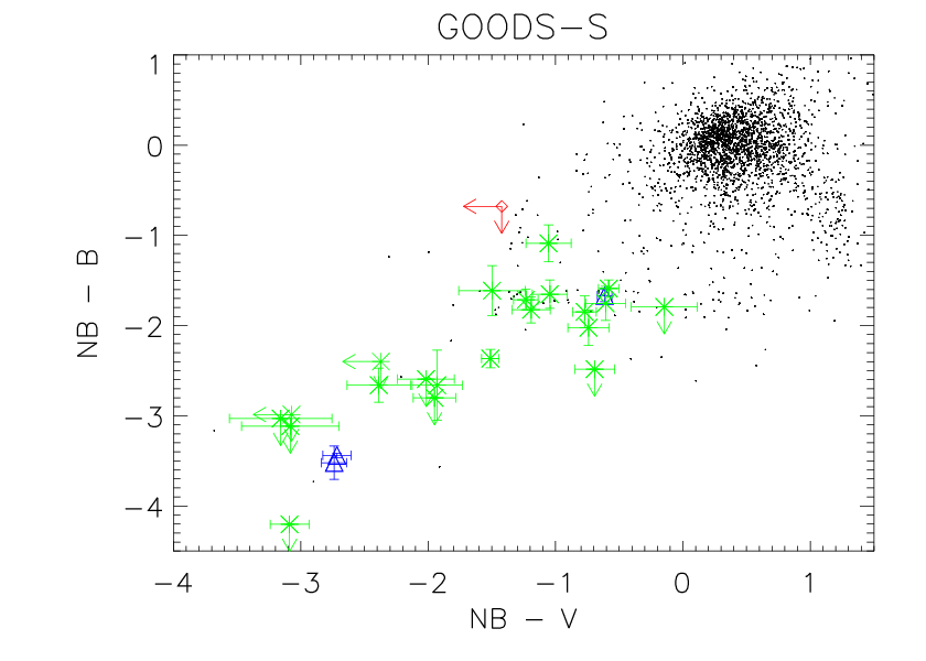

All samples are drawn from survey data-sets such as GOODS-S and HDF-N, hence there is no bias in photometry. In the plot, we see that the LEGO candidates are drawn from a fainter sub-sample of the high-redshift galaxy population. However, for the brighter candidates among our sample, the LEGOs appear to have UV colours similar to LBG galaxies.

3.8 Conclusion
We have performed deep narrow-band imaging of part of the GOODS-S field. The image revealed a set of 24 LEGO candidates, at a redshift of . Of these, three candidates have been observed spectroscopically and are confirmed. The spatial distribution of the candidates appear to be in a filamentary structure, with a 4 confidence, however to confirm this and to plot the filament in 3D-space, we would need spectroscopic redshifts. We have studied the entire candidate sample in all bands available from X-rays to infrared in the GOODS-S data-set. From the SED fitting we conclude that the LEGOs on average have low metallicity (), have stellar masses in the range of M⊙ and low dust extinction (A). The candidates have ages in the range of 100 – 900 Myrs . We also find one galaxy, LEGO_GOODS-S#16, which is best fit by a dusty starburst galaxy at with Ly-emission escaping from an area slightly offset from the central core.
The comparison to a sample of -band drop-out galaxies in the GOODS-S field show that the colours of LEGOs are consistent with the selection criteria for -band drop-outs except they are too faint to be detected from their continuum flux. They also have colours similar to those of LBGs at redshift . In agreement with previous results (e.g. Gawiser et al. 2006), we conclude that Ly-emitters at redshift are dust- and AGN-free, star-forming galaxies with small to medium masses.
Chapter 4 Ly emitters with VISTA
4.1 Introduction
In this chapter, I describe a project which started in February 2005. The idea was to make use of the large field-of-view of the camera of a future telescope called VISTA (Visible and Infrared Survey Telescope for Astronomy), described further in the next section, to find very high redshift () Ly emitters through narrow-band imaging in the near-infrared. The cost of such filters made this a rather expensive project and funding for the filters very generously came from two sources; IDA – Instrumentcenter for Dansk Astrofysik (DK) and the Dark Cosmology Centre (DK). In the spring of 2006, we extended the science case to involve all emission-lines (H, [OIII], H and [OII]) and eventually submitted a proposal for a Public Survey with VISTA, entitled “ELVIS – Emission Line galaxies with VISTA Survey”. This proposal was well received by the ESO Public Survey Panel, but was asked to merge with a number of other surveys, with the aim to observe small, but deep, areas of the sky with broad-band filters. Thus, ELVIS was merged into the Ultra-VISTA survey. I have been involved in all steps of this project, from the original idea to ordering/inspecting the filters, and from proposal writing to the accepted Public Survey. The following sections include a short introduction to VISTA, a section on the design and procuration of the filters and a description of the ELVIS Survey. This project also highlighted the need for better estimates of number densities of very high redshift Ly emitters. The results of such a project are presented in Chapter 5.
4.2 VISTA – Visible and Infrared Survey Telescope for Astronomy
New advances in technology will always prompt new surveys of the night-time sky. The first large area sky survey in the near infrared, the Two Micron Sky Survey (TMSS; Neugebauer & Leighton 1969), was carried out in the 1960’s and the next large area survey did not happen until the late 1990’s with the 2MASS Survey (Skrutskie et al. 2006) covering the entire sky in the three main bands J, H and Ks. A survey called UKIDSS was started in 2005 (Lawrence et al. 2007). It has several parts, both wide/shallow and small/deep fields, all in the Northern Sky. It is on the background of these surveys that VISTA was conceived. VISTA, originally planned to have both an infrared and an optical camera but later designed with only an infrared camera, is an almost (at the time of writing this thesis) completed 4-m. telescope dedicated almost entirely to near-infrared surveys. For this purpose, it has been equipped with an infrared camera array of 16 detectors, covering a field-of-view of 0.6 square degrees in each single exposure, see Fig. 4.1. The detectors are not buttable, i.e. they cannot be placed adjacent to each other, but need to be separated by a large fraction of the width of the detector itself. This is because the detectors interfere with each other if they are too near each other. Thus, to get a continuous mosaic image, the camera needs to be shifted in six different positions (or paw-print, as each single exposure is called). A plot of the resulting exposure time coverage can be seen in the right panel of Fig. 4.2.
The field-of-view (FOV) of each paw-print with VISTA is unprecedented as can be seen in the FOV comparison in the left panel of Fig. 4.2. The image shows the FOVs of current detectors (HST/NICMOS, VLT/ISAAC and UKIRT/WFCAM) and a future detector (VLT/HAWK-I). As in the picture, the VISTA FOV is approximately 3 times the FOV of WFCAM (only northern hemisphere) and 346 times the FOV of ISAAC.
A schematic lay-out of the telescope and camera can be seen in Fig. 4.3 and the technical details of VISTA are given in Table 4.1.
| M1 diameter | 3.95 m. |
|---|---|
| M2 diameter | 1.24 m. |
| f ratio at instrument | 3.25 |
| Mount | Altitude-Azimuth |
| Number of detectors | 16 |
| Type of detector | Raytheon VIRGO HgCdTe 0.84-2.5 micron |
| Number of pixels per detector | |
| Pixel size | /pixel |
| Read-out noise | 20.9 e- |
| Detector Quantum Efficiency | 71 % (J), 74 % (H), 75 % (Ks) |
| Operating temperature of camera | K |
| Available filters | z, Y, J, H, Ks, NB1185 |
A point to note is that the VISTA detector array is stationary in the camera, which has no shutter, and the filters are turned into the light path with a filter wheel. The filter wheel has eight slots, of which one holds a blank plate, six hold the filters mentioned in Table 4.1 and the final slot is empty initially. The fact that there is no shutter makes positioning of filter sets and rotation patterns of the filter wheel crucial. When moving to a blue filter, or a narrow-band filter, it is undesirable to turn the wheel so that the detector array is exposed to the light coming through one of the redder filters, as this will “flash” the array with light and reduce the sensitivity temporarily.


VISTA is funded by PPARC, UK, but operated by ESO. It is placed at the “NTT” peak at Paranal, Chile and will be fully operational by early 2008, according to the plan. The majority, 75%, of VISTAs time is dedicated to Public Surveys, i.e. large scale surveys conducted by the science community where all data, raw and reduced, become public. Six surveys have been approved for the initial five year survey period. An overview of each survey is given in Table 4.2.
| Name | Area (deg2) | Filters | Science case |
|---|---|---|---|
| Ultra-VISTA | 0.9 | Y, J, H, Ks, NB1185 | Very high redshift universe, |
| galaxy formation and evolution, | |||
| very deep, small area survey | |||
| VHS | 20000 | Y, J, H, Ks | Complete, shallow, southern |
| hemisphere map | |||
| VIDEO | 15 | z, Y, J, H, Ks | AGN surveys, galaxy clusters, |
| very massive galaxies | |||
| VVV | 520 | z, Y, J, H, Ks | Galactic bulge and plane, |
| open and globular clusters, | |||
| variable sources | |||
| VIKING | 1500 | z, Y, J, H, Ks | Weak lensing and baryon |
| acoustic oscillations | |||
| VMC | 184 | Y, J, Ks | Survey of the Magellanic system |
4.3 The narrow-band filters
The width of a VISTA narrow-band filter can not be narrower than Å due to the large shifts in wavelengths over the field-of-view, see also sec. 4.3.2. As the sky spectrum in the J band is full of atmospheric OH-lines, there are only a small number of possible wavelengths to place such a filter. These correspond to e.g. 7.73, 8.22, 8.78 etc. The first redshift, and later on the last, are planned to be surveyed with DAzLE (The Dark Ages z Lyman-alpha Explorer, Horton et al. 2004). Our first idea was thus to place the filter at the intermediate redshift. However, it was discovered that this window has a significant [OII]-line in the dark range, and it was discarded as an option. The window corresponding to is quite wide (see Fig. 4.4) and it will only be surveyed by DAzLE at a later stage, hence we chose to place our filter at the wavelength corresponding to , .

4.3.1 Filter specifications
The filter specifications were prepared in the same manner as the original VISTA broad-band filters specifications. The camera array will experience a slight passband shift over the field-of-view due to the filters operating in an f/3.25 beam, and the outer arrays may experience a broadening of % due to a slight field-dependent effect, due to the chief ray being tilted by degrees at the edge of the field. These effects will be especially pronounced with the narrow-band filter, due to the small passband width. We investigated how these effects would influence the filter specifications thoroughly prior to sending out calls for quotations, and found that the effect would not be severe, see sec. 4.3.2. A plot of such a study can be seen in Fig. 4.6. We also anticipated the possibility of extensively measuring the effects during commissioning of the telescope and following that produce corrective algorithms to be used while reducing the data. The specifications made for the filter were thus set to be:
- -
Central wavelength should be 1185 nm 2 nm.
- -
Peak transmission should be at least 75% (Goal: 85%).
- -
The passband FWHM should be 10 nm 2 nm.
- -
The transmission at 1174 nm and 1195 nm should be below 10%.
- -
The transmission at 1165 nm and 1210 nm should be below 1%.
- -
The average transmission between 700 nm and 1140 nm should be below 0.1%.
- -
The average transmission between 1250 nm and 3000 nm should be below 0.01%.
The last point is especially important as “red leaks” are a severe problem with near-infrared narrow-band filters (Sutherland, priv. communication). The call for quotations was sent to four firms in October 2005, and the best bid was made by NDC Infrared Engineering11 1 http://www.ndcinfrared.com/. The filters were subsequently ordered by the Dark Cosmology Centre in January 2006 and 20 filters were delivered to the Rutherford Appleton Laboratory in Oxford, UK, in April 2007, see Table 4.3.
| Filter | CWL (nm) | FWHM (nm) | Maximal T (%) |
|---|---|---|---|
| 911056R5_4 | 1182 | 11.1 | 71 |
| 301106R6_1 | 1183 | 11.6 | 72 |
| 011206R5_1-1 | 1183 | 12.0 | 71 |
| 021206R5_3 | 1184 | 11.0 | 73 |
| 011206R5_1 | 1185 | 11.2 | 70 |
| 260207R5_1 | 1185 | 12.0 | 76 |
| 281106R5_3 | 1185 | 10.7 | 70 |
| 230207R6_3 | 1185 | 11.9 | 74 |
| 080207R6_1 | 1185 | 11.8 | 74 |
| 230207R5_3 | 1186 | 11.5 | 78 |
| 270207R5_4 | 1187 | 12.0 | 70 |
| 260207R5_3 | 1187 | 12.0 | 74 |
| 090207R5_4 | 1188 | 11.6 | 73 |
| 230207R5_5 | 1188 | 11.9 | 76 |
| 050207R6_1 | 1188 | 11.7 | 73 |
| 090207R5_1 | 1188 | 11.8 | 71 |
| 230207R5_2⋆ | 1188 | 11.8 | 73 |
| 230207R6_2 | 1188 | 11.8 | 76 |
| 260207R5_4 | 1188 | 11.9 | 77 |
| 311006R5_1 | 1189 | 10.5 | 76 |
4.3.2 Central wavelength and passband shift
The optical path of VISTA is a converging beam. This means that each pixel on each detector sees an annulus of light coming from the primary mirror and obscured by the secondary mirror. But a pixel at the edge of the filter/detector array has a tilted view of this annulus, i.e. the centre of the annulus is shifted into the actual light annulus. The effect is a cosine function of the length of a vector pointing out a light element in the annulus divided by the refractive index (assumed to be 1.8, Sutherland priv. communication), integrated over the entire annulus. This causes the central wavelength of the filter to shift and the passband to increase.
A schematic of the annulus can be seen in Fig. 4.5. The shifted central wavelength is given by:
| (4.1) |
where
where = 8.75 degrees, = 3.85 degrees and = 1185 nm (Sutherland, priv. communication). This is true for a central pixel at the very centre of the array. For any other pixel, a value of and has to be added to and in the cosine function in the top integral. The largest effect is achieved when , which is at the corner of the field. The effect of the integrated factor is always to decrease the central wavelength and the effect is at its greatest a factor of 0.5 %. The change in wavelength for can be found in Table 4.4 for four positions. These positions correspond to e.g. the positions of detector 6 (number 1 in table), detector 5 (number 2 in table), detector 1 (number 3 in table) and detector 2 (number 4 in table). The shifts are symmetric in each quadrant of the array.
| Shifted wavelength in four points | |
|---|---|
| Point | (nm) |
| Centre | 1182.46 |
| 1 | 1182.34 |
| 2 | 1182.01 |
| 3 | 1181.43 |
| 4 | 1181.76 |
We assume that the filter transmission function is a Gaussian function:
| (4.2) |
where FWHM and central wavelength of the filter. Since the central wavelength shifts over each camera array, the transmission will become broadened and skewed towards a top-hat function. Figure 4.6 show this effect on the corner array in the OH-line free window. The effect is a broadening in FWHM of the order of 10 %.


4.3.3 Inspection of narrow-band filters
In May, 2007, we visited Rutherford Appleton Laboratory (RAL) in order to inspect the filters. Some photographs from the inspection can be found in Fig. 4.8.
During the inspection, performed in the clean room at RAL, we carefully opened each package and checked each filter for the following issues:
- -
Consistency in labelling on wrapping and filter.
- -
Overall condition of filter.
- -
Level of flaking.
- -
Existence of “pinholes”, “comas”, scratches or other damages.
- -
Discolorations.
All filters displayed varying degrees of flaking, i.e. material from the coating at the edges falling off and lying loose in the package. This is very undesirable, as it may scratch the coating if it rubs against the surface. Two filters were mislabeled, or even unlabeled on the filter itself. One filter showed a large discoloration along the edges, indicating that the coating was incomplete around the edges. This filter was removed from the pool of usable filters. A few filters had small chips at the edges, although small enough to not cause any complications. Many filters had small pinholes but they were shallow enough that they can be flat-fielded away (Dalton, priv. communication). Overall, all but the one with a discolored edge were accepted for use.
4.3.4 Positioning of filters in the VISTA filter tray
After studying the transmission curves of the remaining, accepted 19 filters, the three most blue filters were also excluded from further use, and kept as spares, as they overlap significantly with sky emission lines in the blue edge of the sky window, as seen in Fig. 4.4. Thus, with 16 filters left to use we attempted to “puzzle” these filters together so that all detectors along each column of the detector array would have as similar transmission curves as possible, also taking into account the shift that occurs of the field-of-view. The result can be seen in Fig. 4.7.


4.4 ELVIS and Ultra-VISTA
ELVIS is part of Ultra-VISTA, an ESO Public Survey that aims to do very deep near-infrared broad- and narrow-band imaging in one pointing in the COSMOS field (Scoville et al. 2006). The main science case for Ultra-VISTA is to get one of the deepest images to date in the near-IR bands of a large area on the sky. It will focus on detecting the first galaxies at very high redshift and to study faint objects at intermediate redshifts. ELVIS aims specifically at searching for emission-line galaxies at several redshifts in order to study galaxy formation and evolution, at what redshift re-ionisation started as well as the evolution of the cosmic star formation history.
4.4.1 Science goals
As my involvement in Ultra-VISTA is almost solely focused on the ELVIS part, I will here only discuss the science goals of ELVIS. There are a number of arguments why a large scale survey in the infrared for emission line galaxies will yield new and exciting insights into galaxy formation and star formation history. The objective is split into three parts, one looking for very high redshift Ly emitters, and the others to observe H and intermediate redshift emitters.
Ly emitters
The quest for detecting cosmological objects is always pushing to reach further away in redshift space, and further back in time. So far, no objects have been confirmed to be at a redshift larger than seven. Of the objects confirmed to be above redshift six, the vast majority are in fact Ly-emitters. To date, 22 Ly-emitters (Hu et al. 2002; Kodaira et al. 2003; Rhoads et al. 2004; Kurk et al. 2004; Stern et al. 2005a; Taniguchi et al. 2005 and Kashikawa et al. 2006), 13 quasars (Fan et al. 2006; Willott et al. 2007) and one GRB (Haislip et al. 2006) with spectroscopic redshift above six has been published. Another two detections of gravitationally lensed Ly emitters at redshifts around have been suggested in Stark et al. (2007). The reason for the easy detection of Ly-emitters is the relative ease with which they are found (narrow-band imaging) and with which the redshift can be confirmed (spectroscopic follow-up and detection of single emission line). Hence, it is often believed that Ly-emitters will be the most successful tool in discovering even higher redshift sources. Some projects have already started. Three attempts to observe Ly-emitters at redshift have been made (Parkes, Collins & Joseph 1994; Willis & Courbin 2005; Cuby et al. 2006) but the results are null-detections due to too small observed fields and/or to shallow flux limits. The DAzLE project has been presented by Horton et al. (2004). It is designed to find Ly-emitters at redshift and , using a specially made instrument to be placed in visitor focus at the VLT. The DAzLE instrument, however, has a small field of view (x). As these sources will be very under-luminous due to the distance to them, and we thus sample only the top of the Ly luminosity function, the key to finding a large sample of very high redshift galaxies is large survey area and volume. This is the main strength of the VISTA telescope.
There are two main reasons why we wish to observe very high redshift Ly emitters; re-ionisation and galaxy formation studies. Re-ionisation is the epoch of the history of our Universe when its vast amounts of hydrogen gas was ionised after being completely neutral. This happened when the first stars, and potentially the first quasars, lit and galaxies started to form. But it is yet unknown exactly when this event took place. Recent results from studying the cosmic microwave background (CMB) have constrained the upper limit of the re-ionisation redshift to be and observations of galaxies and quasars have set the lower limit to be (e.g. Spergel et al. 2006; Malhotra & Rhoads 2004; Fan et al. 2006). Several authors have argued that Ly-emitting high-redshift galaxies may provide a tool to constrain the redshift of re-ionisation better (e.g. Miralda-Escudé 1998; Miralda-Escudé & Rees 1998; Haiman 2002; Gnedin & Prada 2004; Haiman & Cen 2005). These authors show that absorption in the Gunn-Peterson trough (i.e. the absorption on the short wavelength side of the Ly line due to the intergalactic medium; Gunn & Peterson 1965) may extend to the red side of the Ly emission line and cause damping wings. Haiman (2002) and Haiman & Cen (2005) suggest that this damping will change the shape of the luminosity function of Ly-emitters before and after re-ionisation. McQuinn et al. (2007) suggest that the clustering of very high redshift Ly emitters is an independent and powerful tool to diagnose the level of re-ionisation. With a large sample of Ly-emitters at redshift , it will be possible to analyse the Ly emission line, make a comparison of luminosity functions of Ly-emitters at different redshifts, and determine the level of clustering, thus revealing when re-ionisation happened, or at a minimum placing constraints on the time of re-ionisation.
When it comes to galaxy formation and evolution, possible observables include number density of Ly-emitters, SFR and and clustering effects. An interesting question to answer is how many Ly-emitters existed at a specific time? Taniguchi et al. (2005) study the number densities of several Ly-surveys between to 6.6 and find no evolution with comoving number density. Another key question related to galaxy formation and evolution is that of the shape of the star formation history. Observations at lower redshifts indicate that Ly-emitters are moderately star-forming, dust free galaxies with little or no AGN content. It is thus of interest to investigate if the SFR was different in this class of objects at very high redshift, what percentage of the total star formation happened in this type of galaxy at very high redshift and what the star formation density was at this epoch.
Emission-galaxies at intermediate redshift
At lower redshift, ELVIS will also be sensitive to emission line galaxies with much higher surface density; H at , [OIII] at , H at , and [OII] at . These redshifts span most of the time when the cosmic star formation occurred, associated with the formation of the stars and galaxies we see in the Universe today. The [OIII]-, H-, and [OII]-lines can all be used as tracers of star formation, and [OIII] and [OII] are also frequently used as tracers of AGN and Seyfert galaxies. The line profiles and ratios of these emission lines give information on the kinematics of the emitting gas, and of the properties of the AGN (Heckman et al. 1981; Boroson 2005; Gu et al. 2006). The forbidden oxygen lines are metallicity dependent, but also affected by AGN. Nevertheless, in particular [OII] is still a good tracer of star formation and hence we will have an interesting handle on the star formation density at , which is complementary to broad-band surveys targeting similar redshifts (e.g. Adelberger et al. 2004).
H emitters
H is a one of the best, direct tracers of the instantaneous star formation rate and it is particularly useful as it is relatively unaffected by metallicity and dust extinction. Several authors have attempted to obtain the H luminosity function at redshifts close to , which is believed to be the peak of star formation in the Universe, but sample sizes are still small (e.g. Tresse et al. 2002; Doherty et al. 2006; Hopkins et al. 2000; Yan et al. 1999). Evidence exists for strong evolution in the SFR from redshift zero to one, by perhaps an order of magnitude (Hopkins 2004, and references therein). However, many surveys are limited to the bright end of the luminosity function due to the small sample sizes and it is therefore not clear whether this evolution in global SFR is a property of galaxies with well above average SFRs, or whether it also extends to average SFR galaxies. The H luminosity of normal galaxies is well studied in the local universe. Comparing the full range of H luminosities at higher redshifts to those of local galaxies could therefore provide crucial insight into the evolution of the SFR. Another question recently posed is that of the apparent “downsizing” of star forming galaxies (Cowie et al. 1996; Heavens et al. 2004; Juneau et al. 2005), claiming that more massive galaxies form earlier than less massive galaxies. To date, no survey has simultaneously reached the sensitivity and the area necessary to fully address the questions of global SFR and “down-sizing”. The sensitivity of ELVIS will reach H luminosities more than three orders of magnitude below L*(H). This will enable unprecedented constraints to the H luminosity function at , in particular the value of the faint-end slope which is still a matter of debate, hence giving a direct observational evidence as to whether the “down-sizing” scenario is true or merely an observational bias.
4.4.2 Survey plan
Ultra-VISTA has three parts; a “deep” survey, a “very deep” survey and ELVIS. All parts will observe the COSMOS field (R.A. , Dec (J2000)). The VISTA camera array consists of 16 detectors, placed in a square pattern with large gaps in between, see Fig. 4.1. The gaps can be filled in by shifting the array in a six step pattern. A full mosaic will then be 1.6 sq.degrees. The broad-band components of Ultra-VISTA will observe a full mosaic and four strips respectively. The “deep” survey will observe a full mosaic but the “very deep” survey will only shift the detectors along the y-axis, creating four strips.
For ELVIS, it was debated for some time which configuration to choose; the continuous mosaic or the four strips. The total integration time was assumed to be fixed and so the full mosaic would be more shallow and the configuration with four strips would go deeper. Based on the expected number counts and clustering results (see Chapter 5) it was decided that ELVIS would also observe in four strips but to a deeper flux limit. The expected depths reached by the different Ultra-VISTA surveys can be seen in Table 4.5.
| Deep Survey | ELVIS | Ultra Deep Survey | |||||||
| Filter | Y | J | H | Ks | NB1185 | Y | J | H | Ks |
| Total exp. time (h) | 48 | 48 | 48 | 48 | 180 | 320 | 320 | 320 | 320 |
| 5 depth, AB | 25.7 | 25.5 | 25.1 | 24.5 | 24.1 | 26.7 | 26.6 | 26.1 | 25.6 |
The survey is planned to start early 2008, with a first release to the public about six months later, followed by yearly releases until the survey is completed. If the telescope operates at peak efficiency and Ultra-VISTA is awarded all the time in its RA range, the program will be completed in five years.
4.4.3 Expectations
The expectations, i.e. the expected number of objects detected, in ELVIS is divided into two parts; Ly-emitters, and lower redshift emitters.
Ly emitters
The attempt to predict the number of Ly emitters detected with ELVIS sparked the project presented in Chapter 5, which presents results from two theoretical models of very high redshift Ly emitters; one semi-analytic model based on CDM and one phenomenological model. The semi-analytic model GALFORM has been presented in Le Delliou et al. (2005; 2006) and follows a hierarchical evolution of galaxies. It has been shown to well reproduce the Ly luminosity functions at lower redshifts. The phenomenological model has been presented in Thommes & Meisenheimer (2005) and assumes that Ly luminosity is proportional to star formation rate, which in turn is proportional to the baryonic mass of the galaxy. The results of comparing the two models and extrapolating results at higher redshifts are described in Chapter 5, and for ELVIS the models predict the detection of 3 - 13 Ly emitters.
Lower redshift emitters
To estimate the number of H-emitters that may be found, we use the H luminosity function of Tresse et al. (2002) with H, , and without reddening correction (Doherty et al. 2006). Using this luminosity function in a field of view of 0.9 deg2, with a line flux limit of erg cm-2 s-1 and over a redshift range we calculate that of the order 3500 H-emitters would be detectable. The expected density of intermediate redshift galaxies will probably be smaller than the density of H emitters because of the higher distance moduli and (on average) lower equivalent widths, even though the higher redshift increases the observed equivalent widths. We estimate that it will be possible to detect about an order of magnitude fewer such objects compared to H emitters, hence of the order of 350 intermediate redshift galaxies.
Chapter 5 Predicting results from very high redshift Ly surveys
This paper has been accepted for publication in Astronomy & Astrophysics on 31 August, 2007. The authors are Nilsson, K.K., Orsi, A., Lacey, C.G., Baugh, C.M., & Thommes, E.
5.1 Abstract
Context Many current and future surveys aim to detect the highest redshift () sources through their Lyman-Ly (Ly) emission, using the narrow-band imaging method. However, to date the surveys have only yielded non-detections and upper limits as no survey has reached the necessary combination of depth and area to detect these very young star forming galaxies.
Aims We aim to calculate model luminosity functions and mock surveys of Ly emitters at based on a variety of approaches calibrated and tested on observational data at lower redshifts.
Methods We calculate model luminosity functions at different redshifts based on three different approaches: a semi-analytical model based on CDM, a simple phenomenological model, and an extrapolation of observed Schechter functions at lower redshifts. The results of the first two models are compared with observations made at redshifts and , and they are then extrapolated to higher redshift.
Results We present model luminosity functions for redshifts between and give specific number predictions for future planned or possible narrow-band surveys for Ly emitters. We also investigate what constraints future observations will be able to place on the Ly luminosity function at very high redshift.
Conclusion It should be possible to observe Ly emitters with present or near-future instruments if enough observing time is allocated. In particular, large area surveys such as ELVIS (Emission Line galaxies with VISTA Survey) will be useful in collecting a large sample. However, to get a large enough sample to constrain well the Ly luminosity function, instruments further in the future, such as an ELT, will be necessary.
5.2 Introduction
One of the most promising ways of detecting very high redshift (), star-forming galaxies is via narrow-band imaging surveys targeting Lyman- (Ly). In particular, redshifts and have been extensively surveyed by several groups (e.g. Ajiki et al. 2003; Hu et al. 2004; Shimasaku et al. 2005; Ouchi et al. 2005, 2007; Malhotra et al. 2005; Taniguchi et al. 2005; Tapken et al. 2006; Kashikawa et al. 2006). The current redshift record for a spectroscopically confirmed Ly emitter (LEGO – Ly Emitting Galaxy-building Object; see Møller & Fynbo 2001) is (Iye et al. 2006) although Stark et al. (2007) have suggested the discovery of two LEGOs at and . The reason why narrow-band surveys are restricted to a discrete number of narrow redshift windows is the night sky OH emission lines. According to the OH line atlas of Rousselot et al. (2000), at Ly redshifts ( Å) there are only a few possible wavelengths where a narrow-band filter can fit in between the OH sky lines. These correspond to , , , and . Several future surveys will target these windows in the sky aiming to detect very high redshift galaxies. Three narrow-band surveys for Ly at redshift have already been completed (Parkes, Collins & Joseph 1994; Willis & Courbin 2005; Cuby et al. 2007) but have only yielded upper limits. Future surveys planned for these redshifts include DaZle (Dark Ages Z Lyman- Explorer, Horton et al. 2004) and ELVIS (Emission-Line galaxies with VISTA Survey, Nilsson et al. 2006b). Observations of very high redshift LEGOs have been proposed as an excellent probe of reionisation, through its effects on the Ly emission line profile (e.g. Miralda-Escudé 1998; Miralda-Escudé & Rees 1998; Haiman 2002; Gnedin & Prada 2004), the luminosity function (e.g. Haiman & Cen 2005; Dijkstra, Wyithe & Haiman 2007b) and the clustering of sources (McQuinn et al. 2007).
We here focus on Ly emission from star-forming galaxies, where the Ly photons are emitted from gas which is photo-ionised by massive young stars. During recent years, theoretical work on Ly emitting galaxies has made significant progress. There are three main aspects to these studies: i) predicting the numbers of star-forming galaxies as a function of star formation rate and redshift, ii) calculating the fraction of the Ly photons which escape from galaxies into the IGM and iii) calculating the factor by which the Ly flux is attenuated by scattering in the IGM on its way to the observer. Accurate treatments of ii) and iii) are complicated because Ly photons are resonantly scattered by hydrogen atoms, with the consequences that absorption of Ly by dust in galaxies is hugely amplified, thereby reducing the escape fraction, and that even a small neutral fraction in the IGM can be effective at scattering Ly photons out of the line-of-sight, thus attenuating the flux. Because of these complications, most theoretical papers have chosen to concentrate on only one aspect, adopting simplified treatments of the other two aspects. Haiman & Spaans (1999) made predictions of the number counts of Ly emitting galaxies by combining the Press-Schechter formalism with a treatment of the inhomogeneous dust distribution inside galaxies. Barton et al. (2004) and Furlanetto et al. (2005) calculated the numbers of Ly emitters in cosmological hydrodynamical simulations of galaxy formation, but did not directly calculate the radiative transfer of Ly photons. Radiative transfer calculations of the escape of Ly photons from galaxies include those of Zheng & Miralda-Escudé (2002), Ahn (2004) and Verhamme, Schaerer & Maselli (2006) for idealised geometries, and Tasitsiomi (2006) and Laursen & Sommer-Larsen (2007) for galaxies in cosmological hydrodynamical simulations. The transmission of Ly through the IGM has been investigated by Miralda-Escudé (1998), Haiman (2002), Santos (2004) and Dijkstra, Lidz & Wyithe (2007a), among others. Several authors (e.g. Haiman, Spaans & Quataert 2000; Fardal et al. 2001; Furlanetto et al. 2005) have studied the effect of cold accretion to describe the nature of so-called Ly blobs (Steidel et al. 2000; Matsuda et al. 2004; Nilsson et al. 2006a), see also sec. 5.7.
Two models in particular, dissimilar in their physical assumptions, have been shown to be successful in reproducing the observed number counts and luminosity functions of Ly emitting galaxies at high redshifts: firstly, the phenomenological model of Thommes & Meisenheimer (2005) which assumes that Ly emitters are associated with the formation phase of galaxy spheroids, and secondly the semi-analytical model GALFORM (Cole et al. 2000, Baugh et al. 2005), which follows the growth of structures in a hierarchical, CDM scenario. The GALFORM predictions for Ly emitters are described in detail Le Delliou et al. (2005, 2006) and Orsi et al. (in prep.), who show that the model is successful in reproducing both the luminosity functions of Ly emitting galaxies in the range and also their clustering properties.
In this paper we aim to provide model predictions to help guide the design of future planned or possible narrow-band surveys for very high redshift Ly emitters. We make predictions based on three approaches: the semi-analytical and phenomenological models already mentioned, and an extrapolation from observations at lower redshift. In section 5.3 we describe the different models used to make the predictions, and in section 5.4 we present the predicted number counts and comparisons with observed luminosity functions at lower redshifts. In section 5.5 we make number predictions for some specific future surveys. A brief discussion regarding what can be learned from these future surveys is found in section 5.6. We give our conclusions in section 5.7.
Throughout this paper, we assume a cosmology with km s-1 Mpc-1, and , apart from the mock surveys discussed in section 5.6, which use GALFORM models matched to the cosmology of the Millenium Run (Springel et al. 2005), (which has km s-1 Mpc-1, and ).
5.3 Models
We use three different approaches to predict the numbers of high redshift () Ly emitters. The models are based on very disparate assumptions. The first model is the semi-analytical model GALFORM (Le Delliou et al. 2005, 2006), the second is the phenomenological model of Thommes & Meisenheimer (2005), and the third model is based on directly extrapolating from observational data at lower redshifts.
Both the semi-analytical and phenomenological models assume that the fraction of Ly photons escaping from galaxies is constant, and that the IGM is transparent to Ly. The simple expectation is that before reionisation, the IGM will be highly opaque to Ly, and after reionisation it will be mostly transparent. However, various effects can modify this simple behaviour; e.g. Santos (2004) finds that the transmitted fraction could be significant even before reionisation, while Dijkstra, Lidz & Wyithe (2007a) argue that attenuation could be important even after most of the IGM has been reionised. The WMAP 3-year data on the polarisation of the microwave background imply that reionisation occurred in the range (Spergel et al. 2007), i.e. the IGM may be mostly transparent to Ly at the redshifts of most interest in this paper. In any case, what is important for predicting fluxes of Ly emitters is the product of the escape fraction from galaxies with the attenuation by the IGM. The two effects are in this respect degenerate.
5.3.1 Semi-analytical model
The semi-analytical model GALFORM (Cole et al. 2000; Baugh et al. 2005), which is based on CDM, has been shown to be successful in reproducing a range of galaxy properties at both high and low redshift, including Ly emitters in the range (Le Delliou et al. 2005; 2006). A full description of GALFORM is given in these earlier papers, so we only give a brief summary here. GALFORM calculates the build-up of dark halos by merging, and the assembly of the baryonic mass of galaxies through both gas cooling in halos and galaxy mergers. It includes prescriptions for two modes of star formation – quiescent star formation in disks, and starbursts triggered by galaxy mergers – and also for feedback from supernovae and photo-ionisation. Finally, GALFORM includes chemical evolution of the gas and stars, and detailed stellar population synthesis to compute the stellar continuum luminosity from each galaxy consistent with its star formation history, IMF and metallicity (see Cole et al. 2000 for more details). The unextincted Ly luminosity of each model galaxy is then computed from the ionising luminosity of its stellar continuum, assuming that all ionising photons are absorbed by neutral gas in the galaxy, with case B recombination.
The semi-analytical approach then allows us to obtain the properties of the Ly emission of galaxies and their abundances as a function of redshift, calculating the star formation histories for the entire galaxy population, following a hierarchical evolution of the galaxy host haloes. In addition, when incorporated into an N-body simulation, we also obtain spatial clustering information. This model has been incorporated into the largest N-body simulation to date, the Millennium Simulation (Springel et al. 2005), to predict clustering properties of Ly galaxies. These results will be presented in a forthcoming paper (Orsi et al., in prep.).
The version of GALFORM which we use here is the one described in Baugh et al. (2005) and Le Delliou et al. (2006), with the same values for parameters. The parameters in the model were chosen in order to match a range of properties of present-day galaxies, as well as the numbers of Lyman Break and sub-mm galaxies at . We assume a Kennicutt IMF for quiescent star formation, but a top-heavy IMF for starbursts, in order to reproduce the numbers of sub-mm galaxies. The only parameter which has been adjusted to match observations of Ly emitters is the Ly escape fraction, which is taken to have a constant value , regardless of galaxy dust properties. Le Delliou et al. (2006) show that the simple choice of a constant escape fraction predicts luminosity functions of Ly emitters in remarkably good agreement with observational data at . Le Delliou et al. (2006) also compared the predicted Ly equivalent widths with observational data at , including some model galaxies with rest-frame equivalent widths of several 100Å, and found broad consistency. For this reason, we use the same value for making most of our predictions at . However, since the value of the escape fraction at is a priori uncertain in the models (e.g. it might increase with redshift if high redshift galaxies are less dusty) we also present some predictions for other values of .
Reionisation of the IGM affects predictions for the numbers of Ly emitters in deep surveys in two ways: i) feedback from photo-ionisation inhibits galaxy formation in low-mass halos and ii) reionisation changes the opacity of the IGM to Ly photons travelling to us from a distant galaxy, as discussed above. GALFORM models the first effect in a simple way, approximating reionisation as being instantaneous at redshift (see Le Delliou et al. 2006 for more details). We assume , in line with the WMAP 3-year results (Spergel et al. 2007). As was shown in Le Delliou et al. (2006; see their Fig. 8), as far as the feedback effect is concerned, varying over the range does not have much effect on the bright end of the Ly luminosity function most relevant to current and planned surveys. For example, varying between 7 and 10 changes the predicted luminosity function at erg s-1 by less than 10% for .
5.3.2 Phenomenological model
The phenomenological model of Thommes & Meisenheimer (2005; TM05 hereafter) assumes that the Ly emitters seen at high redshift are galaxy spheroids seen during their formation phase. We summarise the main features here, and refer the reader to TM05 for more details. The model is normalised to give the observed mass function of spheroids at , which is combined with a phenomenological function that gives the distribution of spheroid formation events in mass and redshift. Each galaxy is assumed to be visible as a Ly emitter during an initial starburst phase of fixed duration (and Gaussian in time), during which the peak SFR is proportional to the baryonic mass and inversely proportional to the halo collapse time. The effects of the IMF and the escape fraction on the Ly luminosity of a galaxy are combined into a single constant factor (i.e. the escape fraction is effectively assumed to be constant). With these assumptions, the luminosity function of Ly emitters can be computed as a function of redshift. The free parameters in the model were chosen by TM05 to match the observed number counts of Ly emitters at (analogously to the choice of in the GALFORM model). This model does not include any effects from reionisation.
5.3.3 Observational extrapolation
Our third approach is to assume that the Ly luminosity function is a Schechter function at all redshifts, following
| (5.1) |
and to derive the Schechter parameters , and at high redshifts by extrapolating from the observed values at lower redshifts. For our extrapolation, we use fits to observations at redshift (van Breukelen et al. 2005; Gronwall et al. 2007; Ouchi et al. 2007), (Ouchi et al. 2007), (Dawson et al. 2007), (Malhotra & Rhoads 2004; Shimasaku et al. 2006; Ouchi et al. 2007) and (Malhotra & Rhoads 2004; Kashikawa et al. 2006), as found in Table 5.1.
| Ref | Redshift | ||||
|---|---|---|---|---|---|
| 1 | |||||
| 2 | 3.1 | ||||
| 3 | 3.1 | ||||
| 3 | 3.7 | ||||
| 4 | 4.5 | ||||
| 5 | 5.7 | ||||
| 6 | 5.7 | ||||
| 3 | 5.7 | ||||
| 5 | 6.5 | ||||
| 7 | 6.5 | ||||
We make linear fits to and vs , and extrapolate to higher redshift. For simplicity, we assume a fixed faint end slope of . We do not make any corrections for any possible effects of reionisation or IGM opacity. The extrapolated values are given in Table 5.2.
| Redshift | |||
|---|---|---|---|
| 7.7 | |||
| 8.2 | |||
| 8.8 | |||
| 9.4 | |||
| 12.5 | |||
5.4 Luminosity functions
The possible Ly redshifts between and where a narrow-band filter can be placed are and . Redshifts beyond 10 are unreachable with ground-based instruments of the near-future. However, one possibility for surveys may be the James Webb Space Telescope (JWST, see section 5.5.3) and so we also make predictions for redshift .
First, we compare the Ly luminosity functions predicted by the semi-analytical (GALFORM) and phenomenological (TM05) models with current observational data at . This comparison is shown in Fig. 5.2, where we compare the models with the cumulative luminosity functions measured in several published surveys at and . We can see that both models match the observational data reasonably well, once one takes account of the observational uncertainties. The error bars on the observational data points, omitted in the plot in order to not confuse the points, are large, at the bright end of the luminosity function due to small number statistics, and at the faint end due to incompleteness in the samples. The shallow slopes at the faint ends of the Taniguchi et al. (2005) and Ouchi et al. (2007) luminosity functions may be due to spectroscopic incompleteness. Both models fit the observations well. Hence we conclude that both of these models can be used to extrapolate to higher redshifts.
We now have three methods of extrapolating to higher redshifts, when the direct extrapolation of the Schechter function from lower redshifts is included. In Fig. 5.3 we plot the predicted luminosity functions at , 8.8 and 12.5 computed by these three methods. For other redshifts, the curves may be interpolated. For GALFORM, we show predictions for the standard value of the escape fraction in the left panel, and for a larger value in the right panel. This illustrates the sensitivity of the predictions to the assumed value of at high redshift. The predictions from the other two models are plotted identically in both panels, since they do not explicitly include the escape fraction as a parameter. GALFORM predictions for the numbers of Ly emitters at were also given in Le Delliou et al (2006). We can see that the predictions from the different methods are fairly similar at , but gradually diverge from each other with increasing redshift. For the highest redshift, , the TM05 model fails in producing a prediction due to numerical problems. We note that making predictions for is challenging, for several reasons. Even though only Myrs separate the ages of the Universe between redshift 8.8 and 12.5, the Universe went through an important transition at this time as reionisation occurred (Spergel et al. 2007). However, we do not know exactly how and when this happened. Also, during this epoch the structure in the dark matter (and hence also in galaxies) was building up very rapidly. This underlines the interest of obtaining observational constraints at these redshifts.
The hatched regions in Fig. 5.3 show the region of the luminosity function diagram that has been observationally excluded at by Willis & Courbin (2005) and Cuby et al. (2006). The former survey was deeper but in a smaller area, whereas the latter was more shallow over a larger area, hence the two-step appearance of the hatched area. From the plot, it is obvious that their non-detections are perfectly consistent with our theoretical models, although the GALFORM model with the non-standard escape fraction is marginally excluded.
5.5 Future surveys
In this section, we discuss more specific predictions for several planned and possible future surveys. For all calculations, we assume a simple selection on the flux of the Ly emission line, with no additional selection on the equivalent width (i.e. we include all galaxies with ). We also assume no absorption by the neutral hydrogen in the IGM which would reduce the measured fluxes and for GALFORM predictions we assume an escape fraction of . The predictions from the GALFORM and TM05 models for these future surveys as well as some published surveys are summarised in Table 5.3.
5.5.1 DaZle – Dark ages z Lyman-Ly Explorer
DaZle is a visitor mode instrument placed on the VLT UT3 (Horton et al. 2004). The instrument is designed to use a narrow-band differential imaging technique, i.e. observing the same field with two very narrow filters with slightly offset central wavelength. Objects with LyLy in one of the filters can then be selected from the differential image of both filters. The field-of-view of DaZle is and it is expected to reach a flux level of erg s-1 cm-2 (5) in 10 hours of integration in one filter. This corresponds to a luminosity limit at redshift of erg s-1. The two initial filters are centred on and (with widths and 0.025 respectively) and at this redshift, the surveyed volume becomes Mpc3 per pointing per filter pair. Thus, from Fig. 5.3, we can conclude that DaZle will discover candidates at with one pointing and filter pair.
5.5.2 ELVIS – Emission Line galaxies with VISTA Survey
ELVIS11 1 www.astro.ku.dk/kim/ELVIS.html is part of Ultra-VISTA, a future ESO Public Survey with VISTA22 2 www.vista.ac.uk (Visible and Infrared Survey Telescope for Astronomy). Ultra-VISTA is planned to do very deep near-infrared broad- and narrow-band imaging in the COSMOS field. It will observe four strips with a total area of 0.9 deg2. The narrow-band filter is focused on the sky background window with central wavelength nm, and redshift width . The flux limit of the narrow-band images is expected to reach erg s-1 cm-2 (5) after the full survey has been completed. Ultra-VISTA will run from early 2008 for about 5 years and all the data will be public. ELVIS is presented further in Nilsson et al. (2006b). ELVIS will survey several different emission-lines (e.g. H at redshift , [OIII] at redshift and [OII] at redshift ) as well as the LyLy line.
When the survey is complete, the final mosaic will reach a LyLy luminosity limit of erg s-1. The volume surveyed will be Mpc3. From Fig. 5.3 we see that ELVIS should be expected to detect LEGOs at .
5.5.3 JWST
A possibility even further into the future is to use the James Webb Space Telescope33 3 www.jwst.nasa.gov (JWST). JWST is scheduled for launch in 2013 and will have excellent capabilities within the near- and mid-infrared regions of the spectrum. Two of the instruments aboard JWST could be used for narrow-band surveys; NIRCam, the near-infrared camera, and TFI, the tunable filter imager (for a review on JWST see Gardner et al. 2006). NIRCam will have 31 filters, of which nine are narrow-band filters. The filter with shortest wavelength has central wavelength m (F164N; , ). TFI will have tunable filters with variable central wavelength, however it is only sensitive at wavelengths larger than m. NIRCam is expected to reach a flux limit of erg s-1 cm-2 (5) in s of exposure time. Hence, a flux limit of erg s-1 cm-2 (5, erg s-1) could be reached in 10 hours, assuming that the sensitivity is proportional to the square root of the exposure time. TFI is expected to be able to reach a flux limit almost a factor of two deeper in the same time, however it has a field-of-view of only half of the NIRCam (which is ). In one NIRCam pointing at redshift , approximately Mpc3 are surveyed. Again, from Fig. 5.3, we can estimate that we will detect galaxies per 10-hour pointing with NIRCam. However, the number of detections depends strongly on the escape fraction which is unknown at such high redshifts, and thus the number of detected galaxies can be larger.
5.6 Constraints on the early Universe
Of the surveys at these redshifts that have been presented in previous articles (Horton et al. 2004; Willis & Courbin 2005; Cuby et al. 2006; Nilsson et al. 2006b), or are conceivable (JWST, see section 5.5.3) only ELVIS will detect a large enough sample to start to measure the luminosity functions and the extent of reionisation at these redshifts and to study the fraction of PopIII stars in the population. We here discuss these issues with respect to ELVIS.
From the semi-analytical modelling, we can make mock observations of the ELVIS survey. The procedure to produce these catalogues is explained in detail in Orsi et al. (in prep.), but the outline of the process is that galaxies from GALFORM are placed in matching dark matter haloes in the Millenium N-body simulation (Springel et al. 2005), which is a cubical volume in a CDM universe of comoving size 500 Mpc/, thus creating a mock universe with simulated galaxies which includes all the effects of clustering. We can then make mock observations of this simulated Universe, including the same limits on flux, redshift, sky area etc. as for any real survey, and from these observations produce mock galaxy catalogues. From the mock catalogues, we can in turn make mock luminosity functions of Ly emitters at redshift . In Fig. 5.1 we plot the “observed” luminosity functions in the 112 mock catalogues taken from different regions of the Millenium simulation volume. Note that for making these mock catalogues, GALFORM was run with the same cosmological parameters as in the Millenium simulation itself, which are slightly different from the “concordance” values assumed elsewhere in this paper, as described in the Introduction (this is why the mean luminosity function for the whole simulation volume which is plotted in Fig. 5.1 is slightly different from the GALFORM prediction for plotted in Fig. 5.3). We used escape fraction .

The figure shows that the spread in number density between the different mock catalogues is large, almost a factor of ten in number density in each luminosity bin. This is a consequence both of the small numbers of galaxies in the mock surveys and of galaxy clustering, which causes “cosmic variance” between different sample volumes. The prediction from GALFORM is therefore that it will be difficult to accurately measure the luminosity function of Ly emitters at even using the sample from the large area ELVIS survey. In particular, there will be no useful constraint on the faint-end slope . This is simply a consequence of the flux limit of narrow-band surveys, i.e. even if we use the median values of the luminosity function from all the mocks, then Schechter functions with slopes in the range to all give acceptable fits, as illustrated in Fig. 5.1. However, if all the data are combined in one luminosity bin, it should be possible to measure assuming values for and . The possibility of including data points from several surveys at different luminosities (e.g. also lensing surveys that probe the faint end of the luminosity function) would also significantly improve the results.
Two suggested methods of constraining reionisation from observations of Ly emitters, without requiring spectroscopy, are to measure the clustering of Ly-sources and to compare the Ly and UV continuum luminosity functions at these redshifts (Kashikawa et al. 2006; Dijkstra, Wyithe & Haiman 2007b; McQuinn et al. 2007). McQuinn et al. (2007) show that large HII bubbles may exist during reionisation, and that these will enhance the observed clustering of Ly emitters in proportion to the fraction of neutral hydrogen in the Universe. A sample of emitters will be enough to constrain the level of reionisation using this effect (McQuinn, priv. communication), almost within reach of the ELVIS survey. A future, extended version of ELVIS would be able to place very tight constraints on reionisation. In Kashikawa et al. (2006) and Dijkstra, Wyithe & Haiman (2007b) the use of the combination of the UV and Ly LFs to constrain the IGM transmission is explored. Ly emission will be much more susceptible to IGM absorption than the continuum emission and thus the ratio between the two LFs will give information on the level of IGM ionisation. However, with increasing redshift for Ly, the continuum emission will be increasingly difficult to observe, and it is unclear if this method will be feasible for surveys such as ELVIS.
It is possible that galaxies at still have a significant population of primordial PopIII stars. A test for the fraction of primordial stars is the amount of HeII 1640 Å emission (Schaerer 2003; Tumlinson, Schull & Venkatesan 2003). Depending on models, these authors predict that the HeII 1640 Å emission line should have a flux between % of the flux in the Ly line. For ELVIS Ly emitters, the HeII 1640 Å line is redshifted to m. Due to the many OH sky emission lines in this region of the spectrum, it would be desirable to try to observe the HeII 1640 Å line from a space-based observatory such as JWST. According to the JWST homepage, NIRSpec will achieve a sensitivity in the medium resolution mode on an emission line at m of erg s-1 cm-2 () for an exposure time of s (30 hours). Thus, if the Ly emission line has a flux of erg s-1 cm-2, the HeII 1640 Å will be marginally detected with JWST in 30 hours of integration, depending on the ratio of HeII 1640 Å to Ly flux. The NIRSpec sensitivity increases at longer wavelengths, but the increasing luminosity distance to galaxy candidates with HeII 1640 Å emission at longer wavelengths will most likely counteract this effect.
5.7 Discussion
We summarise our predictions for number counts of Ly emitters in narrow-band surveys in Fig. 5.4. We also summarise the numbers of detected objects for specific current and future surveys in Table 5.3.
| Name | Area | Luminosity limit | GALFORM | TM05 | Observed | ||
| (arcmin2) | (5, erg s-1) | number | |||||
| SXDS-O | 5.7 | 8100 | 443 | 339 | 515 | ||
| SXDS-S | 5.7 | 775 | 112 | 86 | 83 | ||
| SXDS-K | 6.5 | 918 | 108 | 57 | 58 | ||
| DaZle | 7.7 | 47 | 0.45 | 0.16 | — | ||
| ELVIS | 8.8 | 3240 | 20 | 2.8 | — | ||
| Cuby06 | 8.8 | 31 | 0.0003 | 0.0 | 0 | ||
| W&C05 | 8.8 | 6.3 | 0.015 | 0.002 | 0 | ||
| JWST | 12.5 | 9.3 | 0.018 | — | — | ||
A few comments can be made on the differences in predictions between the two models. Firstly, as can be seen in Fig. 5.4 and also Fig. 5.3, the luminosity functions have steeper faint-end slopes in the GALFORM models than in the TM05 models. Secondly, the GALFORM and TM05 models predict similar amounts of evolution at a given flux over the range where they can be compared.
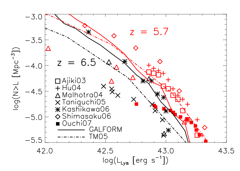

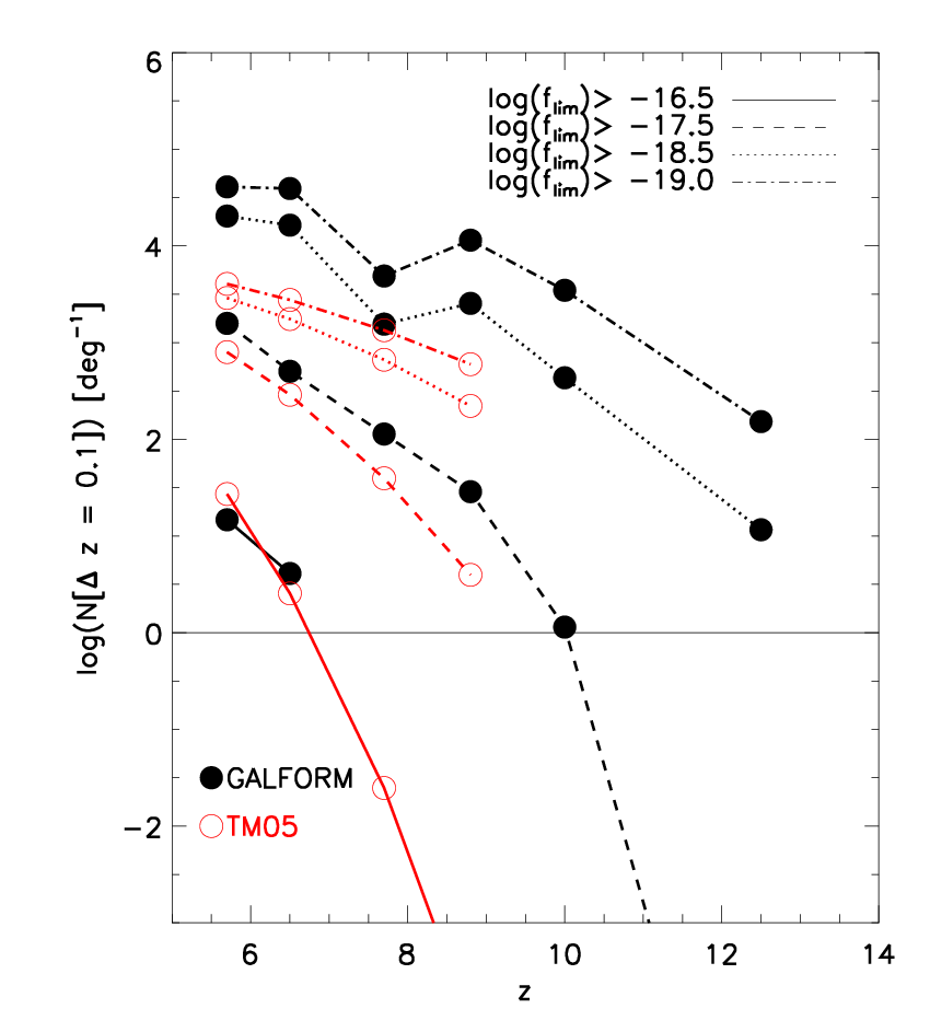
Several factors enter into the error bars of our predictions. One problem is the uncertainties in, and disagreement between, the observed lower redshift luminosity functions which are used to calibrate the theoretical models. There are many caveats in producing Ly luminosity functions, of which the selection function is the most difficult to correct for. The problem arises from that the filter transmission curve is not box-shaped, but rather gaussian. Thus, only brighter objects will be observed at the wings of the filter, and these will be observed to have smaller than intrinsic luminosities. Secondly, the equivalent width (EW) limit that the survey is complete to depends on the depth of the broad-band images used for the selection. Thirdly, if the sample is a photometric sample, it is possible that there are lower redshift interlopers, where the emission line is e.g. [OII], in the sample. Finally, the samples are still so small that we have to deal with small number statistics. All of these problems cause the observed luminosity function at lower redshifts to be uncertain.
Both theoretical models (semi-analytical and phenomenological) have uncertainties resulting from how they model the galaxy formation process, and also from the assumption that the fraction of Ly photons escaping from galaxies is constant and does not change with redshift. In addition, neither model includes attenuation of the Ly flux due to neutral hydrogen in the IGM. This attenuation would be expected to be strong at , when the IGM is neutral, and weaker at , when most of the IGM is ionised. The degree of attenuation depends on a number of different effects, as analysed in Santos (2004), and discussed in Le Delliou et al. (2006), and is currently very uncertain. Nonetheless, this attenuation is expected to produce observable effects on the evolution of the Ly luminosity function, if reionisation occurs within the redshift range covered by future observations, and so estimating the reionisation redshift and the neutral fraction after reionisation are included in the science goals of these surveys.
It is apparent that the key to acquiring a large sample of Ly-emitting galaxies at redshifts greater than 7 is both depth and area. In a recent paper, Stark, Loeb & Ellis (2007) suggest that one of the most efficient means of finding very high redshift Ly emitters is through spectroscopic surveys focused on gravitational lensing clusters. Lensing surveys could easily reach down to a luminosity limit of erg s-1 in a few tens of hours. However, the surveyed volumes are very small, of the order of a hundred Mpc3. For a lensed survey, the area in the source plane is reduced by the same factor that the flux is amplified, so in principle one gains in the total number of objects detected relative to an unlensed survey if the luminosity function is steeper than . In the GALFORM and TM05 models, the asymptotic faint-end slope is shallower than this, but at higher luminosities, the slope can be steeper. For example, GALFORM predicts that at , the average slope in the luminosity range – erg s-1 is close to (see Fig. 8 in Le Delliou et al. 2006), so that a lensing amplification of 10 results in 10 times more objects being detected, with intrinsic luminosities 10 times lower, compared to an unlensed survey with the same area and flux limit. Therefore lensing and narrow-band surveys are complementary to each other as they probe different parts of the luminosity function. With either type of survey, reaching a significant sample of redshift should be possible in the next few years with telescopes/instruments in use or soon available.
An interesting type of object found recently in narrow-band surveys are the Ly blobs, large nebulae with diameters up to 150 kpc and Ly luminosities up to erg s-1 with or without counterpart galaxies (e.g. Steidel et al. 2000; Matsuda et al. 2004; Nilsson et al. 2006a). Several mechanisms have been proposed to explain this phenomenon, including starburst galaxies and superwinds, AGN activity or cold accretion. It is interesting to consider if such objects would be detected in any of these surveys, assuming they exist at these redshifts. A typical Ly blob will have a luminosity of erg s-1 and a radius of, say, 25 kpc. This will result in a surface brightness of erg s-1 kpc-2. Thus, a narrow-band survey will have to reach a flux limit, as measured in a radius aperture of erg s-1 at redshift , corresponding to . (An aperture radius of around is expected to be roughly optimal for signal-to-noise.) For lower or higher redshifts, this limit is higher or lower respectively. Thus, ELVIS will not be able to detect Ly blobs unless they are brighter and/or more compact at higher redshift than a typical blob at lower redshift. DaZle and JWST could in principle detect this type of object, but only if they are very abundant in the very high redshift Universe, due to the small survey volumes of these instruments. It is of course highly uncertain what properties such Ly blobs would have at , or their space density, but it appears unlikely that the future surveys presented here would detect any such objects.
To find compact Ly emitters at redshifts in significant numbers we will probably have to await instruments even further in the future. If a future 40-m ELT (Extremely Large Telescope) was equipped with a wide-field NIR imager and a narrow-band filter of similar width to ELVIS, it could reach a luminosity limit of erg s-1 at redshift (where a suitably large atmospheric window exists) in approximately 20 hours. Using the GALFORM model for , the number density should be N(L) Mpc-3 at this luminosity limit. Thus, to get a sample of ten Ly emitters would require imaging an area on the sky of approximately 16 square arcminutes, assuming a narrow-band filter with redshift range . This could be achieved with one pointing if the detector has a field-of-view of 6 arcmin on a side, as suggested by the ESO ELT Working Group44 4 http://www.eso.org/projects/e-elt/Publications/ELT_INSWG_FINAL_REPORT.pdf. It should of course be noted that these are very tentative numbers, but they display the possibilities of far future instruments.
Chapter 6 Selection methods for Ly emitters
This paper is in preparation. The authors will be Nilsson, K.K., Möller, O., Hayes, M., Møller, P., & Fynbo, J.P.U.
6.1 Abstract
Context Narrow-band surveys for Ly emitters is an increasingly popular method to find high redshift galaxies. However, different groups have presented different methods to find Ly galaxy candidates. We here present a method to determine the best selection criteria, combining narrow- and broad-band observations.
Aims To find the optimal selection sub-space in colour-colour space for Ly emitters, i.e. to determine the best colour selection criteria for this type of object.
Methods We simulate a galaxy population by constructing a large number of galaxy spectra and convolve with filter profiles to get the “observed” fluxes. Some spectra have Ly emission superposed, which is then observed through a narrow-band filter profile. We study the distribution in dimensional colour space and attempt to find the angle in which the scatter in the normal galaxy population is the least and the emission-line candidates are most easily and most accurately selected.
Results We present the three most favourable combinations of galaxy colours to be used to select i) Ly emitters from field galaxies and ii) Ly emitters from [OII] emitters. We also present the optimal selection criteria to use with these colours.
Conclusions All of the best combinations of colours for selecting Ly emitters from field galaxies include sampling the UV slope of the galaxy with two broad-band filters, one on either side of the Ly line. It is concluded that selection with two narrow-band/broad-band colours is superior to selection with only one narrow-band/broad-band colour.
6.2 Introduction
Narrow-band imaging surveys have become increasingly successful in discovering high and very high redshift galaxies. There are now in total several hundreds of spectroscopically confirmed Ly emitters at redshifts (e.g. Steidel et al. 2000; Fynbo et al. 2003; Matsuda et al. 2005; Venemans et al. 2007; Nilsson et al. 2007), (Finkelstein et al. 2007), (Malhotra et al. 2005; Shimasaku et al. 2006; Tapken et al. 2006) and (Taniguchi et al. 2005; Kashikawa et al. 2006). Most candidates are selected using one narrow-band filter and one broad-band filter, where objects that are bright in the narrow-band filter but comparatively faint or non-detected in the broad-band filter are selected. In some cases, the selection is based on determining the equivalent width (EW) of the potential emission line. However, the calculation of the EW of an emission-line observed through a narrow-band/broad-band filter set-up has been shown to be uncertain (Hayes & Östlin 2006). In 1993, Møller & Warren (1993) suggested for the first time that two colours should be used for detecting emission-line galaxies, i.e. that any object should be observed with a narrow-band filter and two broad-band filters. This method was subsequently explored in Fynbo et al. (2003) and Nilsson et al. (2007). However, present day and future multi-wavelength surveys such as e.g. the GOODS (Giavalisco et al. 2004) and COSMOS (Scoville et al. 2006) surveys warrant a review on the selection criteria for narrow-band surveys in fields where public, multi-wavelength data exists.
This Letter is organised as follows; in section 6.3 we present the models we use to create colour plots for “normal” galaxies and Ly emitters as well as the method by which we find the most efficient selection colours. In section 6.4 we present our results and in sections 6.5 we discuss the results and draw conclusions.
Throughout this paper, we assume a cosmology with km s-1 Mpc-1 (Freedman et al. 2001), and . Magnitudes are given in the AB system.
6.3 Method
6.3.1 Creating a mock sample
To study which selection criteria are most successful in determining Ly emitter candidates, we create model spectra using the Starburst99 models (Leitherer et al. 1999; Vázquez & Leitherer 2005). For the “normal” galaxy population, we create spectra, evenly covering the parameter space given in Table 6.1.
| Min. value | Max. value | Number of steps | ||
|---|---|---|---|---|
| Redshift (z) | 0 | 3 | 50 | |
| Dust (E(B-V)) | 0 | 1 | 20 | |
| Age (Gyr) | 0.001 | 10 | 50 (log) | |
The age of each model galaxy is constrained to be less than the age of the Universe at the redshift it is at. The mass of a galaxy is a simple multiplication factor and as we here only work with colours, i.e. flux ratios, the mass is irrelevant except in the cases when the mass is so small that the flux in a certain waveband is lower than the flux detection limit. We discuss this further in sec. 6.5. All spectra are calculated using single stellar populations (SSP), i.e. all the stars are created instantaneously. This will cause the spectrum to be blue to the extreme at a young age and red to the extreme when old, thus widening the distribution of the field galaxy population with respect to other more extended SFHs. Particularly at late times colours will be redder, with fewer hot stars present in the population.
For the Ly emitters, we create galaxy spectra with the same range of ages and dust amounts as for the field galaxies and redshift them to the redshift in question. We then add Ly by calculating the expected H EW from the age of the starburst, convert this to a Ly EW using case B recombination (Brocklehurst 1971) and add such a line to the model spectra. The Ly EWs range between Å (Charlot & Fall 1993). As we are also interested in distinguishing between Ly emitters and interloper galaxies such as [OII]-emitters, we also add an [OII]-emission line to a sample of galaxy spectra with EWs ranging between Å, as [OII] is the most common interloper in Ly emission surveys. We create Ly emitters and [OII] emitters respectively. We wish to decide the optimal selection criteria for a variety of Ly redshifts, see Table 6.2, that have been or will be surveyed.
| Redshift (zLyα) | Reference (e.g.) | |
|---|---|---|
| 2.4 | Francis et al. 2004 | |
| 3.1 | Nilsson et al. 2007 | |
| 4.5 | LALA; Finkelstein et al. 2007 | |
| 5.7 | Shimasaku et al. 2006 | |
| 6.5 | Kashikawa et al. 2006 | |
| 7.7 | DaZle; Horton et al. 2004 | |
| 8.8 | ELVIS; Nilsson et al. 2006b | |
For each galaxy spectrum, we convolve the spectrum with a set of standard filter transmission curves in order to calculate magnitudes and colours. The filters used correspond, for broad-bands, to the filter set used in the GOODS Surveys, see Table 6.3 and Fig. 6.1, and are very similar to standard Johnson-Cousins filters. The narrow-band filters are defined to be gaussian shaped, with central wavelength centred on the particular Ly redshift desired and with full-width half-maximum (FWHM) of 1% of the central wavelength.
| Filter name | Central Wavelength | FWHM | |
|---|---|---|---|
| (ESO 2.2-m) | 3630 Å | 760 Å | |
| (F435W, HST) | 4297 Å | 1038 Å | |
| (F606W, HST) | 5907 Å | 2342 Å | |
| i (F814W, HST) | 7764 Å | 1528 Å | |
| (F850LP, HST) | 9445 Å | 1230 Å | |
| (VLT) | 1.25 m | 0.6 m | |
| (VLT) | 1.65 m | 0.6 m | |
| (VLT) | 2.16 m | 0.6 m | |
| (Spitzer) | 3.58 m | 0.75 m | |
| (Spitzer) | 4.50 m | 1.02 m | |
| (Spitzer) | 5.80 m | 1.43 m | |
| (Spitzer) | 8.00 m | 2.91 m | |

6.3.2 Optimal distinction of Ly emitters
In past work (e.g. Fynbo et al. 2003; Nilsson et al. 2007) a distinction between Ly emitting candidates and non-emitters was performed by making a colour cut in two narrow- minus broad-band colours. The reasoning was that, due to the emission in the narrow-band (NB) filter, the difference between Ly emitters and non-emitters should be maximal. However, this was based on a purely qualitative argument, rather than a careful analysis. In this Letter we want to perform a more quantitative study using the evolutionary models developed. The data at hand are three populations of galaxies with, in total, 78 colour combinations created from mock magnitudes in the bands presented in Table 6.3 combined with a NB filter. Thus, we wish to discriminate between three populations of galaxies in a 78 dimensional space. The goal is to find two colours in which the populations can be plotted where the largest separation between the three populations occur. We choose two colours as this allows a significant number of combinations - more than one colour - but does not require a large amount of additional data for the selection.
For each combination of colour, the catalogues of galaxies is smoothed using a gaussian filter onto a grid with a step size of in magnitude difference. We then optimise the selection of Ly emitters by calculating a “merit” number which is the ratio of distance between the mean colour of each population over the area of the overlap between the populations, see Eq. 6.1.
| (6.1) |
In this equation, are the colours and is the area covered by the population in colour space. The best selection colours will have the highest merit number . To calculate the optimum, we need to know the distribution of samples of both populations. This can in principle be obtained observationally. However, in the case here, for our evolutionary models, we do not have that information. The sample of normal galaxies will for example outline a region in the parameter space where outliers are extreme types of galaxies. Within these boundaries, we do not know the actual number distribution of galaxies in the colour space. Rather we assume that within the region covered by the boundaries, the distribution is uniform.
6.4 Results
For each redshift, all combinations in two dimensions that include the narrow-band magnitude in both combinations (in order to minimise the number of observed bands needed) are ranked according to their merit number, , as described in the previous section. We also run the code with only [OII]-emitters and Ly emitters with the aim to find an optimal combination of colours for separating the two types of emitters photometrically. For the emitters, we make a number of cuts in the properties of the spectra. We set the maximum age of a Ly emitter to be 40 Myrs and the maximum age of an [OII] emitter to be 100 Myrs. The maximum E(B-V) allowed is for both Ly and [OII] emitters. Also, for both populations of emitters, the minimum EW of the emission line is taken to be 10 Å.
An illustration of the best combinations for redshift can be seen in Fig. 6.2.


The plot shows the top combinations of colours to select between Ly emitters and field galaxies or [OII] emitters. As can be seen, the overlap is very small with the field galaxy population. The overlap between the two emitter populations is larger. The best three selection combinations for our selected redshifts can be found in Table 6.4. In this table, the merit number has been normalised to the most favourable value for each redshift. The merit number for the distinction between Ly emitters and [OII]-emitters has been calculated the same way as for the distinction with field galaxies.
| Best solution | Second solution | Third solution | |
| Ly emitters vs. Field galaxies | |||
| 2.4 | NB-U vs. NB-B (1.00) | NB-B vs. NB-V (0.85) | NB-B vs. NB- (0.67) |
| 3.1 | NB-B vs. NB-V (1.00) | NB-V vs. NB- (0.86) | NB-B vs. NB- (0.83) |
| 4.5 | NB-B vs. NB-J (1.00) | NB-B vs. NB-Ks (1.00) | NB-B vs. NB-H (1.00) |
| 5.7 | NB-U vs. NB-H (1.00) | NB-B vs. NB-H (0.76) | NB-B vs. NB- (0.76) |
| 6.5 | NB-U vs. NB-H (1.00) | NB-V vs. NB-H (0.83) | NB-V vs. NB- (0.83) |
| 7.7 | NB-U vs. NB-Ks (1.00) | NB-B vs. NB-H (0.93) | NB-B vs. NB-Ks (0.93) |
| 8.8 | NB-B vs. NB-Ks (1.00) | NB-V vs. NB-Ks (0.55) | NB- vs. NB- (0.37) |
| Ly emitters vs. [OII]-emitters | |||
| 2.4 | NB-U vs. - (1.00) | NB-U vs. NB-B (0.98) | NB-B vs. -i (0.93) |
| 3.1 | NB- vs. U-B (1.00) | NB-Ks vs. U-B (0.57) | NB- vs. U-B (0.57) |
| 4.5 | NB-Ks vs. U-V (1.00) | NB-J vs. B-V (0.51) | NB-Ks vs. B-V (0.51) |
| 5.7 | NB-U vs. V- (1.00) | NB-U vs. V- (1.00) | NB-U vs. V- (1.00) |
| 6.5 | NB-U vs. V- (1.00) | NB-U vs. V- (1.00) | NB-U vs. - (1.00) |
| 7.7 | NB-U vs. U- (1.00) | NB-U vs. U- (1.00) | NB-U vs. B- (0.94) |
| 8.8 | NB-U vs. U- (1.00) | NB-B vs. U- (0.96) | NB-U vs. B- (0.96) |
For each best solution, we also want to find the actual selection criteria to apply. Again, as the actual distribution of galaxies within colour space is unknown, it is impossible to decide different confidence levels at which the criteria can be applied. Instead, the only possibility is to calculate the 100% confidence limit, i.e. where there is no contamination of the two populations. For the best solutions in Table 6.4, these criteria are given in Table 6.5.
| Redshift | Selection criteria (Ly/FG) | |
|---|---|---|
| 2.4 | NB-B (NB-B)(NB-U) | |
| 3.1 | NB-V (NB-V)(NB-B) | |
| 4.5 | NB-J (NB-J)(NB-B) | |
| 5.7 | NB-H (NB-H)(NB-U) | |
| 6.5 | NB-H (NB-H)(NB-U) | |
| 7.7 | NB-K (NB-Ks)(NB-U) | |
| 8.8 | NB-K (NB-Ks)(NB-B) | |
| Selection criteria (Ly/[OII]) | ||
| 2.4 | NB-U | |
| 3.1 | U-B (U-B)(NB-) | |
| 4.5 | U-V (U-V)(NB-Ks) | |
| 5.7 | NB-U (V-)(NB-U) | |
| 6.5 | NB-U (V-)(NB-U) | |
| 7.7 | NB-U (U-)(NB-U) | |
| 8.8 | NB-U (U-)(NB-U) | |
6.5 Discussion
The motivation of this Letter is to study how to best select Ly-emitter candidates photometrically. The necessity of such a review is two-fold; firstly, several surveys have or are being conducted that offer a large set of public, multi-wavelength data in fields or varying size on the sky. These data-sets can be used to make very accurate photometric redshifts and should hence provide excellent opportunities to select Ly emitting candidates from narrow-band surveys with great accuracy. Secondly, narrow-band surveys will try to reach fainter fluxes and larger area/samples at all redshifts, and also to much higher redshifts (). In both cases spectroscopic follow-up to confirm the candidates can be challenging or even beyond the capacity of spectrographs. Without spectroscopic confirmation, it is necessary to make very accurate photometric selections with as few interlopers as possible.
Hence, we have here reviewed the most efficient colour combinations that can be made with a large multi-wavelength data-set for selecting Ly emitters from field galaxies, as well as distinguishing between Ly emitters and [OII]-emitters. For the first part of the results, it is interesting to note that all of the best selection criteria for Ly emitters/field galaxies involve one combination with a broad-band filter on the blue side of the narrow-band filter and one combination with a broad-band filter on the red side of the narrow-band filter. For the best combination for all redshifts, the filter on the red side of the Ly line is also always located on the blue side of the Balmer break in the spectrum. This result can be understood intuitively, as two broad-band magnitudes on either side of the Ly line, but both blue-ward of the Balmer break, will constrain the UV slope of the galaxy and thus one easily gets a measure of the equivalent width of the emission line when this value is combined with the narrow-band flux.
For redshift the best selection colour is identical to what has been used in other publications (Fynbo et al. 2003; Nilsson et al. 2007). Fynbo et al. (1999; 2002) have also used a two-colour approach in trying to find Ly emitters at redshifts . They applied the colours NB-U and NB- with successful results. This criteria is similar to the third best solution that we find for redshift . At other redshifts, the method of selecting emitters using two filters has not previously been used. However, it is obvious from our results that a selection with two colours including narrow-band/broad-band combinations is better than a selection with only one narrow-band/broad-band colour as is most commonly used. This is obvious since our method finds selection criteria for all redshifts (in Table 6.5) where both colours are included. If one colour would be the best selection combination, the criteria would have been a cut parallel to either the or axis. This is not the case. This is also an intuitive result. More information will always yield a more accurate result. In future work it would be interesting to further quantify how much better results a two colour selection yields compared to a one colour selection.
As for the distinction between Ly emitters and [OII] emitters, for several redshifts the best selection requires the narrow-band minus U band colour. This is presumably because Ly emitters with redshifts above should at all times have extremely faint emission in U, as this filter will sample the far-UV, whereas [OII]-emitters are at lower redshift and will thus have continuum emission in the observed U filter.
The method used here of maximising the merit number has the advantage that it is very simple to calculate and to understand. It also involves very few bands, in our case only three for the selection between Ly emitters and field galaxies, and so it can be applied to almost any survey. The disadvantage is that for large multi-wavelength surveys such as GOODS or COSMOS, it does not make use of all the data available. Better solutions may be found if more bands are allowed. The method is not very rigorous mathematically, nor is it a simple task to define the merit number. A more careful analysis would take a more complex approach, using a principal component analysis such as e.g. Fisher Linear Discriminants (Fisher 1936).
A caveat with the input to the method is the unknown mass distribution. In order to facilitate the calculations made here, all galaxies were assumed to have a mass of . The catalogues were also cut at a magnitude of mag which introduces another arbitrary cut in mass properties. Thus, we do not know the actual distribution of galaxies in colour space, and we will miss extreme cases of colours in low or high mass galaxies. The next step would thus also be to try to incorporate a mass function of galaxies into the model. Yet another caveat is the lack of understanding of the properties of Ly emitters and [OII] emitters. The true age and dust content distribution of these galaxies are not known. Previous SED fitting of Ly emitters have shown them to be in general young, low mass and dust free (Gawiser et al. 2006; Lai et al. 2007; Finkelstein et al. 2007; Nilsson et al. 2007). However, this may be a selection bias arising from the selection criteria which often include high EW and blue colours. Finally, in future work it would be desirable to try to incorporate the effects of IGM opacity in the spectra. This effect will be most important at very high redshifts, but also very uncertain as we have no conclusive information about how and when re-ionisation happened.
Chapter 7 Conclusions
The technique of finding high redshift galaxies through their Ly emission and narrow-band imaging, and hence the class of high redshift galaxies called Ly emitters, is a relatively young branch of observational cosmology. Even though it was suggested already by Partridge & Peebles in 1967, the first successful observations did not occur until the beginning of the 1990’s. Since the year 2000, many Ly emitters have been published though, reaching in total more than 500 spectroscopically confirmed galaxies between redshift , including the highest redshift galaxy recorded to date at (Iye et al. 2006). The relative ease with which this type of galaxy can be found, i.e. with moderate exposure times on medium sized to large telescopes, promises to make this technique one of the best selection techniques for future high and very high redshift galaxy surveys. This in turn will enable a better understanding of the young Universe and galaxy formation and evolution through the study of these galaxies, and an insight into the so-called “Dark Ages”, before the Universe was re-ionised.
However, although the sample of Ly emitters is steadily growing, relatively little is known about the nature of these galaxies, or their relation to other classes of high redshift galaxies. In the first part of this thesis, we attempt to study a sample of redshift Ly emitters found through narrow-band imaging in GOODS-S, a field with a large amount of public, multi-wavelength data (Chapter 2 and 3). The main objective to get this narrow-band image was to use the multi-wavelength data to try to understand the nature (e.g. the masses, ages, star formation rates, redshift distribution and spatial distribution) of these galaxies, and to compare their properties to those of other classes of high redshift galaxies. In part, this goal has been achieved. The following main results have been presented in this thesis.
- •
SED fitting analysis: properties of Ly emitters at
In Chapter 3, the multi-wavelength data was used to perform an SED fitting of the spectra of the Ly emitters, thus allowing a study of their properties, including stellar mass, metallicity and dust content. We found that the stacked SED of these Ly-emitters, which covered the spectra of the galaxies from the restframe far-UV to restframe near-infrared, was best fitted by a very low metallicity (), had low dust extinction (), medium ages ( Gyrs) and medium stellar masses (M M⊙). These results are in reasonably good agreement compared to results from other studies (Gawiser et al. 2006; Lai et al. 2007; Finkelstein et al. 2007), see also Table 1.3. In one respect our results differ from the others; our age is higher. However, the age of an SED is the parameter which is the hardest to constrain, as can also be seen in Fig. 3.7. Thus, relatively little weight should be put on these differences, as well as the actual ages themselves.
To expand on the work presented in the paper in Chapter 3, we here evaluate the mass function of our Ly emitters. The properties cited above are for the stacked SED, hence a sort of average of all the properties of all candidates. It is interesting to consider what the distribution of masses for these objects look like. To do this, we take the mass derived from the SED fitting, multiply it with the number of objects in the stack (this number is 23) and calculate individual masses by assuming that the stellar mass of the galaxy is proportional to the band luminosity. The reason for choosing the band as a mass estimator is because it is in this band that we have the largest signal-to-noise detections of the candidates. This is not the best estimator, as the observed band corresponds to the restframe UV and the galaxy light in this regime can be heavily absorbed by dust, i.e. a more massive galaxy with a large amount of dust would appear smaller in this calculation. However, it is the only band in which we can do this analysis, as it is the only band with adequate signal-to-noise and most detections. The resulting distribution can be seen in the histogram plot in Fig. 7.1.

It appears that a large fraction, more than 20%, of the total mass of the sample is concentrated to one object (LEGO_GOODS-S#14), and more than half the sample has masses below M M⊙. With these results in mind, it will be of great interest in the future to try to improve the statistics on this kind of Ly emitter mass function, to see if this type of massive Ly emitters are very rare occurrences or if they are more abundant. Whatever the result, it can be said with certainty that the majority of Ly emitters have small masses.
We can compare the results of our SED fitting with similar results from LBG surveys. Three such surveys have been published in Papovich, Dickinson & Ferguson (2001), Shapley et al. (2001) and Verma et al. (2007). In all papers, the authors use samples of spectroscopically confirmed LBGs at redshift or respectively. They use Bruzual & Charlot (2003) models, with a Calzetti extinction law and metallicity fixed at solar levels. They fit for star formation history, dust, age and stellar mass. The median results for the sample of 74 LBGs presented in Shapley et al. (2001) are , age Myrs and M M⊙. Papovich, Dickinson & Ferguson (2001) find similar results, but with a larger dust content of up to . Verma et al. (2007) find their LBGs to be less massive (M M⊙) and younger, but with larger star formation rates. To compare the dust results, one has to take into account that the ratio between and is . Thus, the dust extinction in the LBGs of Shapley et al. (2001) is approximately , in good agreement with the results of Verma et al. (2007). This is similar, or a bit higher than the value found in Chapter 3. The ages of the LBGs are slightly lower than those of the Ly emitters, although this is a difficult quantity to constrain, as discussed above. Finally, a large difference also lies in the stellar masses. LBGs at are much more massive than Ly emitters at the same redshift. Another difference is the star formation rate. Papovich, Dickinson & Ferguson (2001), Shapley et al. (2001) and Verma et al. (2007) all find star formation rates in the range of a few ten to several hundred solar masses per year, whereas we find star formation rates less than ten solar masses per year. Thus, there is a clear difference in the properties of LBGs and Ly emitters at this redshift; LBGs are more massive, more star forming and possibly more dusty than Ly emitters although the two types of galaxies have similar ages.
- •
LEGO_GOODS-S#16: A Ly emitting dusty starburst galaxy?
During the analysis of the multi-wavelength data of the candidates in the GOODS-S field, we discovered one candidate with a very unusual SED profile, LEGO_GOODS-S#16. This candidate was undetected in the bluest band, the HST band, and marginally detected in the band with the greatest signal-to-noise. But as we followed the candidate in the redder bands, its flux increased dramatically, see also Fig. 3.9. Although with a small offset between Ly and counterpart centroid, it appears as if this is a very dusty starburst galaxy with Ly emission emerging from one side. We are hoping to follow this detection up with future mm/sub-mm observations, that could hopefully give more insight into the nature of this anomalous object.
- •
Discovery of filamentary structure: Two parallel filaments at
A further result from that paper was the discovery of a filamentary structure, consisting of two, seemingly parallel filaments stretching beyond the length of the image. Filaments have been observed before (Møller & Fynbo 2003; Matsuda et al. 2005), but never two parallel filaments. It would be of great interest to get spectroscopy of the candidates in order to confirm the structure, and plot it in three dimensions. Ultimately, further imaging at the ends of the filament would be interesting, to map out the structure completely.
- •
First detection of cold accretion: a Ly blob in GOODS-S
In Chapter 2 we present the discovery of a Ly blob. This blob has an angular diameter of up to kpc and a Ly line luminosity of almost erg s-1. After studying the complete set of deep multi-wavelength data available, we saw that this blob, unlike all other published blobs, had no obvious optical/infrared counter-part. It was realised, after taking all possible explanations into account, that this was the first observed Ly blob that could only be described by cold accretion in a satisfactory way.
- •
ELVIS: a promising future survey for very high redshift Ly emitters
A large part of the time during my PhD has been spent on the project which evolved into “ELVIS”. The initial phase of the project included writing numerous applications for funding of the filters and observing time. I was also involved in the designing of the filters and the initial contacts with the filter producing companies. At later stages, I was involved in writing a Public Survey proposal and in the testing of the filters. After comparing the survey parameters (i.e. area, flux limit expected, filter specifications) of different near-infrared surveys for very high redshift Ly emitters, including ISAAC surveys, DaZle, ELVIS, JWST etc., it is clear that ELVIS will be one of the best opportunities to observe the very high redshift Universe. The combination of large area (0.9 deg2) and relatively deep flux limit for a near-infrared narrow-band image ( erg s-1 cm-2) should enable ELVIS to detect a few times ten Ly emitters at . These detections can be used to study galaxy formation and will probably give one of the best constraints on re-ionisation at this redshift from observed high redshift galaxies. Moreover, the survey will produce a vast catalogue of H emitters, as well as other emission line objects at intermediate redshift. This catalogue will be a treasure for anyone interested in studying the star formation and metallicity history of the Universe and galaxy evolution in general. Again, this sample will be gathered in the COSMOS field, a field with a vast amount of public, multi-wavelength data, including the very deep near-infrared data collected by Ultra-VISTA. This will enable further multi-wavelength studies of, in particular, the lower redshift galaxy sample.
- •
Predictions for very high redshift Ly surveys
In Chapter 5 we studied very high redshift Ly luminosity functions. This was a follow-up work from the preparatory work done for ELVIS. In this chapter, we extrapolate two published theoretical models for Ly emitters at lower redshifts to higher redshifts. We also try to extrapolate the parameters of observed Ly luminosity function fits to Schechter functions. The result is a plot of luminosity functions which can be used for groups planning future surveys for high redshift Ly. Using these luminosity functions, we made specific number predictions for several present and future narrow-band surveys. The conclusion of the project was that detections of small samples of galaxies are to be expected in the next five years, but to get a good handle on the very high redshift Universe, yet more future observatories will be necessary.
- •
How to best select Ly emitters
In the final chapter of this thesis, Chapter 6, we explore the colour space spanned by a population of mock galaxies, including “normal” galaxies, Ly emitters and [OII]-emitters. The aim of this work in progress is to determine how to best select Ly emitters from a general population of observed galaxies and how to distinguish them from interloper emitters such as [OII]-emitters. The motivation was to see if it is possible to select Ly emitters in a confident way so that spectroscopy is unnecessary, using the strength of present and future public multi-wavelength surveys such as GOODS and COSMOS. In our method, we calculated a “merit number” which quantifies how good any combination of colours is in separating two populations of galaxies. This merit number is related to the projected distance between the two populations and to the area of the overlap between the two projections. As a result, we presented the three best selection combinations to distinguish Ly emitters from field galaxies or [OII] emitters. The conclusion of the project is a set of selection colours and selection criteria that may be used by the community both to find Ly emitters with observed data, as well as when preparing observing proposals. Two interesting results from the project were the conclusions that for selection, two colour combinations including the narrow-band magnitude offer better results than one colour combination and that these two combinations should include a broad-band filter on either side of the Ly line, but both blue-ward of the Balmer break. This is work that will be refined in the future.
Summary
To summarise, in the first part of the thesis, the emphasis was on using the available multi-wavelength data in GOODS-S to study the nature of Ly emitters at . This data turned out to be crucial in several aspects of my work. It was necessary, for instance, to determine that the Ly blob that was detected was indeed the first one to be best explained by cold accretion. This would have been impossible if the broad-band coverage had been smaller. The X-ray and mid-IR data ruled out an AGN nature of the blob and the optical/near-IR data excluded the possibility of a star-forming galaxy. Further, this data was also crucial in performing an accurate SED fitting for the candidates. It is true that many of the bands only included upper limits, but in many cases these limits constrained the SED. Especially the infrared data was useful in the SED fitting, in order to constrain the masses of the objects. It was also using the multi-wavelength data that the special SED of LEGO_GOODS-S#16 was identified as a potential Ly emitting dusty starburst galaxy. If this is confirmed, LEGO_GOODS-S#16 will be the first dusty starburst galaxy detected through its Ly emission. The increase in public multi-wavelength data also prompted the work presented in the final chapter, where we tried to find new selection criteria for Ly emitters at several different redshifts for surveys where a large complimentary data-set is available.
In the second part of this thesis, a project to detect very high redshift () Ly emitters was presented. This is a project which has not yielded any observational results yet, although it prompted the work presented in Chapter 5, where new Ly luminosity functions are derived and discussed in the context of future narrow-band surveys. ELVIS is a project which I am hoping to be part of for the coming years, and which will produce very interesting results within the next five years.
The topic of Ly emitters is a field of research which is growing intensively at the moment, with increasing interest from the science community. It is a very promising method to easily detect high redshift, low luminosity, low mass, dust- and AGN-free star forming galaxies. It is also one of the most, if not the most, promising methods in detecting the highest redshift galaxies in the Universe. In the next chapter I write about what future ideas, plans and hopes I have regarding this subject.
Chapter 8 Future ideas, plans and hopes
The subject of exploring the Universe using Ly as a tool has only begun, but it is increasing in popularity and it is quite imaginable that many new and interesting revelations about galaxy formation will come from this field in the future. A few aspects that I see as being crucial in understanding these galaxies, and which I hope to be able to work on are mentioned here.
Understanding the stellar population in Ly emitters and their role in the scheme of high redshift galaxies.
Today, the sample of confirmed or candidate Ly emitters is growing rapidly. The number of spectroscopically confirmed LEGOs at redshifts between approaches 600 and probably an equal amount of candidates have been presented in the literature. However, the exact nature of these galaxies is not yet known to any great detail. A few papers have attempted SED fitting of the continuum of LEGOs at redshifts (Gawiser et al. 2006; Nilsson et al. 2007), (Finkelstein et al. 2007) and (Lai et al. 2007). Unfortunately, the samples on which these analysis has been done are still very small and larger samples are needed before statistically robust results will come. However, the future is promising. Several large public multi-wavelength surveys are under way. A project that will make a significant improvement in the field is the COSMOS survey at redshift that we have started with the WFI imager in Chile. This study will greatly increase the number of LEGOs with sufficient multi-wavelength coverage for a large statistical study of the continuum SED.
Another burning issue is that of the scheme of high redshift galaxies. There are today many different methods of finding high redshift galaxies, and just as many “classes” of objects; LEGOs, LBGs, DLAs, sub-mm galaxies, GRB host galaxies, DRGs, EROs etc. etc. How are these classes of galaxies related? It has been suggested that LEGOs are the predecessors of LBGs (Stark, Loeb & Ellis 2007) or that they are part of the same population (Giavalisco 2002), but neither suggestion has been proved. And where does the population of Ly emitting and dusty sub-mm galaxies fit in? During which phases of galaxy formation/evolution do galaxies emit Ly? These are very important questions that I hope will be, if not explained, than at least better understood in the next decade.
Understanding how Ly emitters trace Large Scale Structure and using it to derive information about the geometry of the Universe.
LEGOs appear to be very good tracers of the Large Scale Structure (LSS) of the Universe. They have been observed in candidate proto-clusters (Venemans et al. 2007 and references therein) and in filamentary structures (Møller & Fynbo 2001; Matsuda et al. 2005; Nilsson et al. 2007). Are LEGOs more prone to follow LSS than other classes of galaxies? If so, why? If it is true that LEGOs are tracers of LSS, then they could be used as an independent test on cosmological models, as described by Weidinger et al. (2002). Further, large scale surveys such as the COSMOS survey and also specifically designed instruments such as the VIRUS instrument for the HETDEX11 1 www.as.utexas.edu/hetdex survey may be able to make use of this property of LEGOs to draw conclusions about the cosmological parameters that describe our Universe.
Understanding the evolution of Ly emitters with redshift. Are they the same population at different redshifts?
As mentioned earlier, the sample of Ly emitting galaxies now extend between redshifts from 1.8 to almost 9. This covers almost 3 billion years in time, or almost 25% of the age of the Universe. Are the galaxies that emit Ly the same across this period of time, or are they different types of objects? Are the mechanisms that create Ly the same? Yet another question is how LEGOs evolve with time, if they are only short-lived “flares”, or if it is one of many stages in galaxy formation. It would also be interesting to compare the properties of high redshift LEGOs with Ly emitting galaxies in the local Universe. Can we detect Ly emitters at redshift zero? Again, larger samples and better knowledge of the nature of these objects at different redshifts will hopefully add understanding within this subject.
Exploring the star formation history of the Universe.
Ly is a direct tracer of the star formation rate of a galaxy, albeit potentially affected by dust. Hence, using observations of Ly at different redshifts will put constraints on the star formation rate and star formation density history of the Universe. Together with observations from other emission-line galaxies, which are sometimes by-products of narrow-band surveys for Ly, and from other means of estimating star formation rates in galaxies, we can expect to get more and more accurate measurements of the star formation history of the Universe.
Detecting the first stars, understanding the very first stages of galaxy formation and how and when re-ionisation occurred.
LEGOs are truly one of the best tools in detecting the first stars and the first galaxies. As we move to higher and higher redshifts, the continuum of galaxies will become more and more faint and reach a level that is almost impossible to observe with the instruments of today and to some extent of tomorrow as well. However, it has been suggested that the equivalent width of very high redshift galaxy Ly emission can be very high (Schaerer 2003; Dijkstra & Wyithe 2007) due to the Population III stars at those redshifts. It will then be possible to observe Ly emission to very high redshifts, even with todays instruments. ELVIS is one such example. With ELVIS we will hopefully discover a large sample of redshift galaxies and observe the first stages of galaxy formation.
Re-ionisation is also a popular topic of study at the moment. When did it happen? How? Two sources of information about the re-ionisation are conceivable. One is mapping the HII-emission (e.g. Iliev et al. 2002; Furlanetto, Zaldarriaga & Hernquist 2004; McQuinn et al. 2006) in the radio regime and the other one is Ly observations. With ELVIS we will hopefully be able to constrain the level of ionised gas at redshift , providing key information to help improve models of re-ionisation.
In short, the future for Ly studies appears to be bright, with many interesting results to look forward to. I hope I can be part of them.
Bibliography
Adelberger, K.L., Steidel, C.C., Shapley, A.E., et al., 2004, ApJ, 607, 226
Ahn, S.-H., 2004, ApJ, 601, L25
Ajiki, M., Taniguchi, Y., Fujita, S.S., et al., 2003, AJ, 126, 2091
Alonso-Herrero, A., Pérez-González, P.G., Alexander, D.M., et al., 2006, ApJ, 640, 167
Arnaboldi, M., Neeser, M.J., Parker, L.C., et al., 2007, ESO Messenger, 127, 28
Barton, E.J., Davé, R.,; Smith, J.-D.T., et al., 2004, ApJ, 604, L1
Baugh, C.M., Lacey, C.G., Frenk, C.S., et al., 2005, MNRAS, 356, 1191
Bertin, E., Arnouts, S. 1996, A&AS, 117, 393
Bahcall, J.N., 1966, ApJ, 145, 684
Bahcall, N.A., & Soneira, R.M., 1983, ApJ, 270, 20
Birnboim, Y. & Dekel, A., 2003, MNRAS, 345, 349
Blain, A.W., Smail, I., Ivison, R.J., Kneib, J.P., & Frayer, D.T. 2002, Phys. Rep., 369, 111
Bloom, J.S., Djorgovski, S.G., Kulkarni, S.R., & Frail, D.A., 1998, ApJ, 507, L25
Bolzonella, M., Miralles, J.-M., Pelló, R., 2000, A&A 363, 476
Boroson, T., 2005, AJ, 130, 381
Bower, R.G., Morris, S.L., Bacon, R. et al., 2004, MNRAS, 351, 63
Brocklehurst, M., 1971, MNRAS, 153, 471
Bruzual, G.A., & Charlot S., 2003, MNRAS, 344, 1000
Bunker, A.J., Stanway, E.R., Ellis, R.S., & McMahon, R.G., 2004, MNRAS, 355, 374
Calzetti, D., Kinney, A.L., & Storchi-Bergmann, T. 1994, ApJ, 429, 582
Calzetti, D., Meurer, G.R., Bohlin, R.C., et al., 1997, AJ, 114, 1834
Calzetti, D., Armus, L., Bohlin, R.C., et al., 2000, ApJ, 533, 682
Cantalupo, S., Porciani, C., Lilly, S. J., & Miniati, F., 2005, ApJ, 628, 61
Carilli, C.L., & Yun, M.S., 1999, ApJ, 513, L13
Chandrasekhar, S., 1945, ApJ, 102, 402
Chapman S.C., Scott D., Windhorst R.A. et al., 2004, ApJ, 606, 85
Charlot, S., & Fall, S.M, 1993, ApJ, 415, 580
Charlot, S., & Fall, S.M, 2000, ApJ, 539, 718
Cole, S., Lacey, C.G., Baugh C.M., & Frenk, C.S., 2000, MNRAS, 319, 168
Collin, S., 2001, in the lectures given at “GH Advanced Lectures on the Starburst-AGN Connection”, INAOE, June 2000, eds. D. Kunth, I. Aretxaga, astro-ph/0101203
Condon, J.J., 1992, ARAA, 30, 575
Cowie, L.L., Songaila, A., Hu, E.M., & Cohen, J.G., 1996, AJ, 112, 839
Cowie, L.L., & Hu, E.M., 1998, AJ, 115, 1319
Cuby, J.-G., Hibon, P., Lidman, C., et al., 2007, A&A, 461, 911
Dalton, G.B., Caldwell, M., Ward, A.K., et al., 2006, SPIE, 6269, 34
Davis, M., & Wilkinson, D.T., 1974, ApJ, 192, 251
Dawson, S., Rhoads, J.E., Malhotra, S., et al., 2004, ApJ, 617, 707
Dawson, S., Rhoads, J.E., Malhotra, S., et al., 2007, submitted to ApJ, arXiv:0707.4182
Dickinson, M., Giavalisco, M. & the GOODS team, 2001, in “The Mass of Galaxies at Low and High Redshift,” Proceedings of the ESO Workshop held in Venice, Italy, 24-26 October 2001; eds. R. Bender & A. Renzini, p. 324, astro-ph/0204213
Dekel, A. & Birnboim, Y., 2006, MNRAS, 368, 2
Dey A., Bian C., Soifer B.T. et al., 2005, ApJ, 629, 654
Dijkstra, M., Haiman, Z., & Spaans, M., 2006a, ApJ, 649, 14
Dijkstra, M., Haiman, Z., & Spaans, M., 2006b, ApJ, 649, 37
Dijkstra, M., Lidz, A., & Wyithe, J.S.B., 2007a, MNRAS, 377, 1175
Dijkstra, M., Wyithe, S., & Haiman, Z., 2007b, MNRAS, 379, 253
Dijkstra, M., & Wyithe, S., 2007c, MNRAS, 379, 1589
Doherty, M., Bunker, A., Sharp, R., et al., 2004, MNRAS, 354, L7
Doherty, M., Bunker, A., Sharp, R., et al., 2006, MNRAS, 370, 331
Eisenstein, D.J., Zehavi, I., Hogg, D.W., et al., 2005, ApJ, 633, 560
Emerson, J.P., Sutherland, W.J., McPherson, A.M., et al., 2004, ESO Messenger, 117, 27
Fabian, A.C., 1994, ARA&A, 32, 277
Fan, X., Strauss, M.A., Becker, R.H., et al., 2006, AJ, 132, 117
Fardal, M.A., Katz, N., Gardner, J.P. et al., 2001, ApJ, 562, 605
Fernandez, E.R., & Komatsu, E., 2007, submitted to MNRAS, arXiv:0706.1801
Finkelstein, S.L., Rhoads, J.E., Malhotra, S., Prizkal, N., & Wang, J., 2007, ApJ, 660, 1023
Fisher, R. 1936, Annals of Eugenics, 7, 179-188
Francis, P.J., Woodgate, B.E., Warren, S.J. et al., 1996, ApJ, 457, 490
Francis, P.J., Williger, G.M., Collins N.R. et al., 2001, ApJ, 554, 1001
Francis, P.J., Palunas, P., Teplitz, H.I., Williger, G.M., & Woodgate, B.E., 2004, ApJ, 614, 75
Freedman, W.L., Madore, B.F., Gibson, B.K., et al., 2001, ApJ, 553, 47
Fruchter, A. S., Levan, A. J., Strolger, L. et al., 2006, Nature, 441, 463
Fujita, S.S., Ajiki, M., Shioya, Y., et al., 2003, AJ, 125, 13
Furlanetto, S.R., Schaye, J., Springel, V., & Hernquist, L., 2003, ApJ, 599, L1
Furlanetto, S.R., Zaldarriaga, M., & Hernquist, L., 2004, ApJ, 613, 1
Furlanetto, S.R., Schaye, J., Springel, V., & Hernquist, L., 2005, ApJ, 622, 7
Fynbo, J.P.U., Møller, P., & Warren, S.J. 1999, MNRAS, 305, 849
Fynbo, J.P.U., Møller, P., & Thomsen, B. 2001, A&A 374, 443
Fynbo, J.P.U., Møller, P., Thomsen, B, et al., 2002, A&A, 388, 425
Fynbo, J.P.U., Ledoux, C., Møller, P., Thomsen, B., & Burud, I., 2003, A&A, 407, 147
Fynbo, J.P.U., Gorosabel, J., Smette, A., et al., 2005, ApJ, 633, 317
Gallagher, J.S., Hunter, D.A., & Bushouse, H., 1989, AJ, 97, 700
Gardner, J.P., Mather, J.C., Clampin, M., et al., 2006, Space Science Reviews, 123, 485, astro-ph/0606175
Gawiser, E., Van Dokkum, P.G., Gronwall, C., et al., 2006, ApJL, 642, 13
Giavalisco, M., Steidel, C.C., Adelberger, K.L., et al., 1998, ApJ, 503, 543
Giavalisco, M., 2002, ARAA, 40, 579
Giavalisco, M., Ferguson, H.C., Koekemoer, A.M., et al., 2004, ApJ, 600, L93
Gilks, W.R., Richardson, S., & Spiegelhalter, D.J., 1995, Markov Chain Monte Carlo in Practice, Chapman & Hall, ISBN 0412055511
Gnedin, N.Y. & Prada, F., 2004, ApJ, 608, L77
Gorosabel, J., Pérez-Ramírez, D., Sollerman, J., et al., 2005, A&A, 444, 711
Gronwall, C., Ciardullo, R., Hickey, T., et al., 2007, accepted for publication in ApJ, arXiv:0705.3917
Gu, Q., Melnick, J., Fernandes, R.C., et al., 2006, MNRAS, 366, 480
Gunn, J.E., & Peterson, B.A., 1965, ApJ, 142, 1633
Haiman, Z., & Spaans, M., 1999, ApJ, 518, 138
Haiman, Z., & Loeb, A., 1999, ApJ, 519, 479
Haiman, Z., Spaans, M. & Quataert, E., 2000, ApJL 537, L5
Haiman, Z. & Rees, M.J., 2001, ApJ 556, 87
Haiman, Z., 2002, ApJ, 576, L1
Haiman, Z. & Cen, R., 2005, ApJ, 623, 627
Haislip, J.B., Nysewander, M.C., Reichart, D.E., et al., 2006, Nature, 440, 181
Hamilton, A.J.S., 1993, ApJ, 417, 19
Hashimoto, Y., Oemler, A., Lin, H., & Tucker, D.L., 1998, ApJ, 499, 589
Hawkins, E., Maddox, S., Cole, S., et al., 2003, MNRAS, 346, 78
Hayashino, T., Matsuda, Y., Tamura, H., et al., 2004, AJ, 128, 2073
Hayes, M., & Östlin, G., 2006, A&A, 460, 681
Heavens, A., Panter, B., Jimenez, R. & Dunlop, J., 2004, Nature, 428, 625
Heckman, T.M., Miley, G.K., van Breugel, W.J.M. & Butcher, H.R., 1981, ApJ, 247, 403
Hill, G.J., Gebhardt, K., Komatsu, E., & MacQueen, P.J., 2004, in the proceedings of the “THE NEW COSMOLOGY: Conference on Strings and Cosmology; The Mitchell Symposium on Observational Cosmology” conference held in Texas, US, March 2004, ed. R.E. Allen, D.V. Nanopoulos & C.N. Pope, AIPC, 743, 224
Hjorth, J., Sollerman, J., Møller, P., et al., 2003, Nature, 423, 847
Hjorth, J., Watson, D., Fynbo, J.P.U., et al., 2005, Nature, 437, 859
Hogan, C.J., & Rees, M.J., 1979, MNRAS, 188, 791
Holland, W.S., Robson, E.I., Gear, W.K., et al., 1999, MNRAS, 303, 659
Horton, A., Parry, I., Bland-Hawthorne, J., et al., 2004, astro-ph/0409080
Hopkins, A.M., Connolly, A.J., & Szalay, A.S., 2000, AJ, 120, 2843
Hopkins, A.M., 2004, ApJ, 615, 209
Hopkins, A.M., & Beacom, J.F., 2006, ApJ, 651, 142
Hu, E.M., & McMahon, R.G., 1996, Nature, 382, 231
Hu, E.M., Cowie, L.L., & McMahon, R.G., 1998, ApJ, 502, L99
Hu, E.M., Cowie, L.L., McMahon, R.G., et al., 2002, ApJ, 568, L75
Hu, E.M., Cowie, L.L., Capak, P., et al., 2004, ApJ, 127, 563
Iliev, I.T., Shapiro, P.R., Ferrara, A., & Martel, H., 2002, ApJ, 572, L123
Ivison, R.J., Smail, I., Barger, A.J., et al., 2000, MNRAS, 315, 209
Ivison, R.J., Greve, T.R., Serjeant, S. et al., 2004, ApJS, 154, 124
Ivison, R.J., Smail, I., Dunlop, J.S., et al., 2005, MNRAS, 364, 1025
Iye, M., Ota, K., Kashikawa, N. et al. 2006, Nature, 443, 186
Jaunsen, A.O., Andersen, M.I., Hjorth, J., et al., 2003, A&A, 402, 125
Johansson, P.H., Väisänen, P., & Vaccari, M., 2004, A&A, 427, 795
Juneau, S., Glazebrook, K., Crampton, D., et al., 2005, ApJ, 619, L135
Kashikawa, N., Shimasaku, K., Malkan, M.A., et al., 2006, ApJ, 648, 7
Keel W.C., Cohen S.H., Windhorst R.A., Waddington I., 1999, AJ, 118, 2547
Kennicutt, R.C., 1983, ApJ, 272, 54
Kennicutt, R.C., 1998a, ARAA, 36, 189
Kennicutt, R.C., 1998b, ApJ, 498, 541
Keres, D., Katz, N., Weinberg, D.H., & Dave, R., 2005, MNRAS, 363, 2
Klaas, U., Haas, M., Müller, S.A.H., et al., 2001, A&A, 379, 823
Kobayashi, M.A.R., Totani, T., & Nagashima, M., 2007, submitted to ApJ, arXiv:0705.4349
Kodaira, K., Taniguchi, Y., Kashikawa, N., et al., 2003, PASJ, 55, L17
Kova, K., Somerville, R.S., Rhoads, J.E., Malhotra, S., & Wang, J.X., 2007, accepted for publication in ApJ, arXiv:0706.0893
Kudritzki, R.-P., Méndez, R.H., Feldmeier, J.J., et al., 2000, ApJ, 536, 19
Kurk, J.D., Cimatti, A., Serego Alighieri, S.d., et al., 2004, A&A, 422, L13
Lai, K., Huang, J.-S., Fazio, G., et al., 2007, ApJ, 655, 704
Lacy, M., Storrie-Lombardi, L.J., Sajina, A., et al., 2004, ApJS, 154, 166
Landy, S.D., & Szalay, A.S., 1993, ApJ, 412, 64
Landy, S.D., Szalay, A.S., & Broadhurst, T.J., 1998, ApJ, 494, L133
Laursen, P., & Sommer-Larsen, J., 2007, ApJ, 657, L69
Lawrence, A., Warren, S.J., Almaini, O., et al., 2007, MNRAS, 379, 1599
Leitherer, C., Schaerer, D., Goldader, J.D., et al., 1999, ApJS, 123, 3
Le Delliou, M., Lacey, C.G., Baugh, C.M., et al., 2005, MNRAS, 357, L11
Le Delliou, M., Lacey, C.G., Baugh, C.M., & Morris, S.L., 2006, MNRAS, 365, 712
Loeb, A., & Rybicki, G.B., 1999, ApJ, 524, 527
Lowenthal, J.D., Hogan, C.J., Green, R.F., et al., 1991, ApJ, 377, L73
Macchetto, F., Lipari, S., Giavalisco, M., Turnshek, D.A., & Sparks, W.B., 1993, ApJ, 404, 511
Madau, P., 1995, ApJ, 441, 18
Madau, P., Ferguson, H.C., Dickinson, M.E., et al., 1996, MNRAS, 283, 1388
Maier, C., Meisenheimer, K., Thommes, E., et al., 2003, A&A, 402, 79
Malhotra, S., & Rhoads, J.E. 2002, ApJL, 565, L71
Malhotra, R. & Rhoads, J., 2004, ApJ, 617, L5
Malhotra, S., Rhoads, J.E., Pirzkal, N., et al., 2005, ApJ, 626, 666
Maller, A.H. & Bullock, J.S., 2004, MNRAS, 355, 694
Matsuda Y., Yamada T., Hayashino T. et al., 2004, AJ, 128, 569
Matsuda, Y., Yamada, T., Hayashino, T. et al., 2005, ApJ, 634, L125
McCarthy, P.J., 1993, ARAA, 31, 639
McQuinn, M., Zahn, O., Zaldarriaga, M., Hernquist, L., & Furlanetto, S.R., 2006, ApJ, 613, 815
McQuinn, M., Hernquist, L., Zaldarriaga, M., & Dutta, S., 2007, submitted to MNRAS, astro-ph/0704.2239
Meier, D.L., 1976, ApJ, 207, 343
Menzel, D.H, 1926, PASP, 38, 295
Miralda-Escudé, J., 1998, ApJ, 501, 15
Miralda-Escudé, J. & Rees, M.J., 1998, ApJ, 497, 21
Monaco, P., Møller, P., Fynbo, J.P.U., et al., 2005, A&A, 440, 799
Mori, M., Umemura, M., & Ferrara, A., 2004, ApJ, 613, L97
Murayama, T., Taniguchi, Y., Scoville, N.Z., et al., 2007, accepted for publication in ApJ, astroph/0702458
Møller, P., & Warren, S.J., 1993, A&A, 270, 43
Møller P., & Warren S.J. 1998, MNRAS 299, 661
Møller, P., & Fynbo, J.U. 2001, A&A, 372, L57
Møller, P., Warren, S.J., Fall, S. M., Fynbo, J.U.,& Jakobsen, P. 2002, ApJ, 574, 51
Neugebauer, G., & Leighton, R.B., 1969, Two Micron Sky Survey, a Preliminary Catalog (NASA SP-3047; Washington: GPO)
Nilsson, K.K., Fynbo, J.P.U., Møller, P., Sommer-Larsen, J. & Ledoux, C., 2006a, A&A, 452, L23
Nilsson, K.K., Fynbo, J.P.U., Møller, P., & Orsi, A., 2006b, to appear in the ASP Conference proceedings of ’At the Edge of the Universe’, eds. J. Afonso, H. Ferguson and R. Norris, astro-ph/0611239
Nilsson, K.K., Møller, P., Möller, O., et al., 2007, A&A, 471, 71
Ohyama, Y., Taniguchi, Y., Kawabata, K.S. et al., 2003, ApJ, 591, L9
Ouchi, M., Shimasaku, K., Furusawa, H. et al., 2003, ApJ, 582, 60
Ouchi, M., Shimasaku, K., Okamura, S., et al., 2004a, ApJ, 611, 660
Ouchi, M., Shimasaku, K., Okamura, S., et al., 2004b, ApJ, 611, 685
Ouchi, M., Shimasaku, K., Akyiama, M. et al., 2005, ApJ, 620, L1
Ouchi, M., Shimasaku, K., Akiyama, M., et al., 2007, submitted to ApJ, arXiv:0707.3161
Overzier, R.A., Miley, G.K., Bouwens, R.J., et al., 2006, ApJ, 637, 58
Palunas, P., Teplitz H.I., Francis P.J., Williger G.M., Woodgate B.E., 2004, ApJ, 602, 545
Papovich, C., Dickinson, M., & Ferguson, H.C., 2001, ApJ, 559, 620
Parkes, I.M., Collins, C.A., & Joseph, R.D., 1994, MNRAS, 266, 983
Partridge, R.B., & Peebles, P.J.E., 1967, ApJ, 147, 868
Partridge, R.B., 1974, ApJ, 192, 241
Pascarelle, S.M., Windhorst, R.A., Driver, S.P., Ostrander, E.J., & Keel, W.C., 1996, ApJ, 456, L21
Peacock, J.A., 1983, MNRAS, 202, 615
Peebles, P.J.E., 1974, ApJ, 189, L51
Petitjean, P., Pecontal, E., Valls-Gabaud, D., & Charlot, S., 1996, Nature, 380, 411
Pettini, M., Shapley, A.E., Steidel, C.C., et al., 2001, ApJ, 554, 981
Portinari, L., & Sommer-Larsen, J., 2007, MNRAS, 375, 913
Pritchet, C.J., & Hartwick, F.D.A., 1989, ApJ, 320, 464
Pritchet, C.J., & Hartwick, F.D.A., 1990, ApJ, 355, L11
Pritchet, C.J., 1994, PASP, 106, 1052
Pope, A., Borys, C., Scott, D., et al., 2005, MNRAS, 358, 149
Ranalli, P., Comastri, A., & Setti, G., 2003, A&A, 399, 39
Rhee, G.F.R.N., Webb, J.K., Katgert, P., 1989, A&A, 217, 1
Rhoads, J.E., Malhotra, S., Dey, A., et al., 2000, ApJ, 545, L85
Rhoads, J.E., Dey, A., Malhotra, S. et al., 2003, AJ, 125, 1006
Rousselot, P., Lidman, C., Cuby, J.-G., Moreels, G., & Monnet, G., 2000, A&A, 354, 1134
Santos, M.R., 2004, MNRAS, 349, 1137
Schaerer, D., 2003, A&A, 397, 527
Schaerer, D., & Pelló, R., 2005, MNRAS, 362, 1054
Schechter, P., 1976, ApJ, 203, 297
Schmidt, M., 1965, ApJ, 141, 1295
Schmidt, M., 1963, Nature, 192, 1040
Schmitt, H.R., Calzetti, D., Armus, L., et al., 2006, ApJ, 643, 173
Scoville, N., Aussel, H., Brusa, M., et al., 2006, astro-ph/0612305
Shapley, A.E., Steidel, C.C., Adelberger, K.L., et al., 2001, ApJ, 562, 95
Shimasaku, K., Ouchi, M., Okamura, S., et al., 2003, ApJ, 586, L111
Shimasaku, K., Kashikawa, N., Doi, M., et al., 2006, PASJ, 58, 313
Silva, L., Granato, G.L., Bressan, A., & Danese, L., 1998, ApJ, 509, 103
Silverman, J., Green, P., Barkhouse, W., et al., 2005, in the proceedings of the “The X-ray Universe 2005” conference held in San Lorenzo de El Escorial, Spain, September 2005, ed. A. Wilson, p. 795, astro-ph/0511552
Skrutskie, M.F., Cutri, R.M., Stiening, R., et al., 2006, AJ, 131, 1163
Smail, I., 2002, RSPTA, 360, 2697
Smail, I., Chapman, S.C., Blain, A.W., & Ivison, R.J., 2004, ApJ, 616, 71
Sokolov, V.V., Fatkhullin, T.A., Castro-Tirado, A.J., et al., 2001, A&A, 372, 438
Sommer-Larsen, J., 2005, in the proceedings of the “Island Universes: Structure and Evolution of Disk Galaxies” conference held in Terschelling, Netherlands, July 2005, ed. R de Jong (Springer Dordrecht), astro-ph/0512485
Spergel, D.N., Bean, R., Doré, O., et al., 2007, ApJS, 170, 377
Springel, V., White, S.D.M., Jenkins, A., et al., 2005, Nature, 435, 629
Stanway, E.R., Bunker, A.J., McMahon, R.G., et al., 2004, ApJ, 607, 704
Stark, D.P., Ellis, R.S., Richard, J., et al., 2007, ApJ, 663, 10
Stark, D.P., Loeb, A., & Ellis, R.S., 2007, submitted to ApJ, astro-ph/0701882
Steidel, C.C., Giavalisco, M., Pettini, M., Dickinson, M., & Adelberger, K.L., 1996, ApJ, 462, L17
Steidel, C.C., Adelberger, K.L., Dickinson, M., et al., 1998, ApJ, 492, 428
Steidel, C.C., Adelberger, K.L., Giavalisco, M., Dickinson, M., & Pettini, M., 1999, ApJ, 519, 1
Steidel, C.C., Adelberger, K.L., Shapley, A.E., et al., 2000, ApJ, 532, 170
Steidel, C.C., Adelberger, K.L., Shapley, A.E., et al., 2003, ApJ, 592, 728
Stern, D., Yost, S.A., Eckart, M.E., et al., 2005a, ApJ, 619, 12
Stern, D., Eisenhardt, P., Gorjian, V., et al., 2005b, ApJ, 631, 163
Taniguchi, Y., Shioya, Y. & Kakazu, Y., 2001, ApJL 562, L15
Taniguchi, Y., Ajiki, M., Nagao, T. et al., 2005, PASJ, 57, 165
Tapken, C., Appenzeller, I., Gabasch, A., et al., 2006, A&A, 455, 145
Tasitsiomi, A., 2006, ApJ, 645, 792
Thommes, E. & Meisenheimer, K., 2005, A&A, 430, 877
Totsuji, H., & Kihara, T., 1969, PASJ, 21, 221
Tresse, L., Maddox, S.J., Le Fèvre, O. & Cuby, J.-G., 2002, MNRAS, 337, 369
Tumlinson, J., Shull, J.M., & Venkatesan, A., 2003, ApJ, 584, 608
Urry, C.M., & Padovani, P., 1995, PASP, 107, 803
van Breukelen, C., Jarvis, M. J., & Venemans, B. P. 2005, MNRAS, 359, 895
Vázquez, G.A., & Leitherer, C., 2005, ApJ, 621, 695
Venemans, B.P., Kurk, J.D., Miley, G.K., et al., 2002, ApJ, 569, L11
Venemans, B.P., Röttgering, H J A,; Overzier, R A, et al., 2004, A&A, 424, L17
Venemans, B.P., Röttgering, H.J.A., Miley, G.K. et al., 2005, A&A, 431, 793
Venemans, B.P., Röttgering, H.J.A., Miley, G.K., et al., 2007, A&A, 461, 823
Verhamme, A., Schaerer, D., & Maselli, A., 2006, A&A, 460, 397
Verma, A., Lehnert, M.D., Förster Schreiber, N.M., Bremer, M.N., & Douglas, L., 2007, MNRAS, 377, 1024
Villar-Martín, Sanchez, S.F., De Breuck, C., 2005, MNRAS, 359, L5
Willis, J.P. & Courbin, F., 2005, MNRAS, 357, 1348
Wadadekar, Y., Casertano, S., & de Mello, D., 2006, AJ, 132, 1023
Wang, J.X., Rhoads, J.E., Malhotra, S., et al., 2004, ApJL, 608, 21
Warren, S.J., & Møller, P., 1996, A&A, 311, 25
Warren, S.J., Møller, P., Fall, S.M.,& Jakobsen, P., 2001, MNRAS, 326, 759
Weidinger, M.; Møller, P., Fynbo, J.P.U., Thomsen, B., & Egholm, M.P., 2002, A&A, 391, 13
Weidinger, M., Møller, P., Fynbo, J.P.U., 2004, Nature, 430, 999
Weidinger, M., Møller, P., Fynbo, J.P.U., Thomsen, B., 2005, A&A, 436, 825
Willis, J.P. & Courbin, F., 2005, MNRAS, 357, 1348
Willott, C.J., Delorme, P., Omont, A., et al., 2007, submitted to AJ, arXiv:0706.0914
Wilman, R.J., Gerssen, J., Bower, R.G. et al., 2005, Nature, 436, 14
Wolfe, A.M., Turnshek, D.A., Smith, H.E, & Cohen, R.D., 1986, ApJS, 61, 249
Wolfe, A.M., Lanzetta, K.M., Turnshek, D.A., & Oke, J.B., 1992, ApJ, 385, 151
Wolfe, A.M., Gawiser, E., & Prochaska, J.X., 2005, ARAA, 43, 861
Worsley, M.A., Fabian, A.C., Bauer, F.E., et al., 2005, MNRAS, 357, 1281
Yan, L., McCarthy, P. J., Freudling, W., et al., 1999, ApJ, 519, L47
Zanstra, H., 1927, ApJ, 65, 50
Zheng, Z., & Miralda-Escudé, J. 2002, ApJ 578,33
Chapter 9 Appendix: Co-author statements for papers presented in Chapter 2, 3, 5 and 6
Paper I — Chapter 2
A Lyman- blob in the GOODS South field: evidence for cold accretion onto a dark matter halo
by K.K. Nilsson, J.P.U Fynbo, P. Møller, J. Sommer-Larsen & C. Ledoux
Astronomy & Astrophysics, 452, L23-L26 (2006)
In this paper, the observations, image reduction and source extraction were done by J. Fynbo (JF) and P. Møller (PM). The spectroscopic observations were prepared by K. Nilsson (KN). The spectroscopic data was delivered bias subtracted, flat-fielded and wavelength calibrated. KN did the spectrum extraction and stacking, sky subtraction, extraction of 1-D spectrum and flux calibration. KN also did most of the analysis of the multi-wavelength data and the imaging/spectroscopic data available and the photometric redshifts. The calculations in the beginning of the Discussion were made by Jesper Sommer-Larsen (JSL), who also did the simulation of cold accretion described in the Discussion. The text in the paper was mainly written by KN with support from JF and PM, the plots were all made by KN.
![[Uncaptioned image]](0711.2199v1/kim2.png)
![[Uncaptioned image]](0711.2199v1/johan2.png)
| Kim Nilsson | Johan Fynbo |
Paper II — Chapter 3
A multi-wavelength study of Lyman- emitters in the GOODS South Field
by K.K. Nilsson, P. Møller, O. Möller, J.P.U. Fynbo, M.J Michałowski, D. Watson, C. Ledoux, P. Rosati, K. Pedersen & L.F. Grove
Astronomy & Astrophysics, 471, 71-82 (2007)
The results of this paper was based on the same narrow-band imaging as in Paper I, hence the original narrow-band image data reduction was performed by Johan Fynbo (JF) and Palle Møller (PM). The source extraction was performed by Kim Nilsson (KN), as well as counterpart galaxy identification. The spectra were the same as in Paper I, i.e. basic data reductions were supplied from the ESO pipeline but KN performed stacking, sky subtraction, 1-D spectra extraction and flux calibration. All photometry in all bands was made by KN. The discovery of the filamentary structure and the statistical test was performed by KN. For the SED fitting, KN stacked the candidates and extracted photometry of the SED, and also gave input to the SED fitting code. However, the code itself was written by Ole Möller (OM). KN did most of the analysis on LEGO_GOODS-S#16, except for the GRASIL fits which were made by Michal Michałowski (MM). The comparison to LBGs was performed by KN. KN wrote most of the text, excluding small parts of the introduction, counter-part selection (section 2.2 and 2.3) and SED fitting method section (section 5.1). KN made all plots, excluding Fig. 8 and 12.
| Kim Nilsson | Johan Fynbo |
Paper III — Chapter 5
Narrow-band surveys for very high redshift Lyman- emitters
by K.K. Nilsson, A. Orsi, C.G. Lacey, C.M. Baugh & E. Thommes
accepted in Astronomy & Astrophysics
The two models (the semi-analytical and the phenomenological model) used in this paper have been presented in earlier publications and are not new to this work. The calculations made from the semi-analytical model were made by Alvaro Orsi (AO), Cedric Lacey (CL) and Carlton Baugh (CB) and the calculations from the Thommes & Meisenheimer model were made by Eduard Thommes (ET). Kim Nilsson (KN) compared the models with lower redshift results and calculated the fit to the Schechter functions. The calculation for Cosmic Variance for ELVIS were made by AO. The text of the paper was written mainly by KN, except for section 2.1 which was written by AO. KN made all plots except Fig. 3 and 4.
![[Uncaptioned image]](0711.2199v1/alvaro.png)
| Kim Nilsson | Alvaro Orsi |
Paper IV — Chapter 6
Selection methods for Lyman- emitters
by K.K. Nilsson, O. Möller, M. Hayes, P. Møller & J.P.U. Fynbo
in prep.
In this paper, the mock sample of galaxies was created by Matthew Hayes (MH) and the code to calculate the merit number of each combination of selection colours was written by Ole Möller, all with input from Kim Nilsson (KN). KN wrote the text and made the plots. The selection criteria in Table 6.5 were also retrieved by KN.
![[Uncaptioned image]](0711.2199v1/ole.png)
| Kim Nilsson | Ole Möller |