DESY 07-195
Some numerical studies of the evolution
of generalized parton distributions

A characteristic property of generalized parton distributions (GPDs) is their renormalization scale dependence, described by evolution equations whose derivation led to the very discovery of these functions more than a decade ago [1]. On a practical level, the scale dependence of GPDs is of direct importance for the quantitative description of exclusive scattering processes. Moreover, understanding general features of the evolution behavior should be helpful for developing realistic models and parameterizations of GPDs. The question how a given input distribution changes when evolved to higher scales has been addressed in several studies, both numerically and analytically [2, 3, 4, 5, 6, 7, 8]. Further progress has been achieved recently [9, 10] by constructing explicit solutions of the evolution equations with methods that generalize the familiar Mellin moment inversion for parton density functions (PDFs).

The aim of the present contribution is to study a number of aspects in the evolution of GPDs at a numerical level. We will largely concentrate on the value of the GPDs at $x=\xi$, which at leading order in $\alpha_{s}$ determines the imaginary part of scattering amplitudes, and via dispersion relations also gives their real part up to a $\xi$ independent constant [11]. Furthermore we will focus on the region of small $\xi$, where the behavior of distributions can be conveniently approximated by a power-law behavior. We will pay special attention to the mixing between the gluon GPD $H^{g}(x,\xi,t)$ and

$$H^{S}(x,\xi,t)=\sum_{q}^{n_{f}}\,\bigl[H^{q}(x,\xi,t)-H^{q}(-x,\xi,t)\bigr]\,,$$

(1)

whose forward limit

$$H^{S}(x,0,0)=S(x)=\sum_{q}^{n_{f}}\,\bigl[q(x)+\bar{q}(x)\bigr]$$

(2)

is the familiar singlet combination of quark and antiquark PDFs. For comparison we will also consider $H^{u-d}(x,\xi,t)=H^{u}(x,\xi,t)-H^{d}(x,\xi,t)$ as a representative of the non-singlet sector.

After specifying in Sect. 2 the GPD model used as initial condition for the evolution, we devote most of Sect. 3 to a quantitative study of the old question how the ratio of GPDs and PDFs behaves when evolved to higher scales. We shall in addition take a look at the behavior of the GPDs around $x=\xi$. In Sects. 4 and 5 we turn to the dependence of GPDs on the squared momentum transfer $t$. Both theoretical considerations [12] and lattice QCD calculations [13] indicate that this dependence is correlated with the one on the longitudinal variables $x$ and $\xi$. Since evolution affects the $x$ dependence at given $\xi$ and $t$, it also affects the $t$ dependence at given $x$ and $\xi$ in a nontrivial fashion, which we will quantify in two model scenarios.

For our calculations we have used the numerical code of [14], which provides a numerically fast and stable implementation of GPD evolution at leading order (LO) in $\alpha_{s}$. The effects of next-to-leading (NLO) and next-to-next-to-leading order (NNLO) terms in the evolution kernels have been studied [8, 15] and are known to be important, especially at small $\xi$ in the gluon and singlet sector. This should be kept in mind as a caveat when interpreting our results, but we think that a study at LO is still of some relevance. On one hand, the arguments in [5, 7] about the pattern of evolution to higher scales are based on the LO kernels, so that this order is adequate to test the numerical validity of these arguments. On the other hand, evolution effects on the $t$ dependence are barely known at all, and LO results should at least provide a valid starting point for further investigation.

In the evolution kernels and the running coupling we take $n_{f}=4$ for $m_{c}\leq\mu<m_{b}$ and $n_{f}=5$ for $\mu\geq m_{b}$, with the charm and bottom quark masses $m_{c}=1.3\operatorname{GeV}$ and $m_{b}=4.5\operatorname{GeV}$ used in the CTEQ6 parton analysis [16], which we use for calculating the model GPDs at the starting scale of evolution. We furthermore follow the CTEQ6 analysis in taking the two-loop running coupling with $\Lambda^{\smash{(4)}}=326\operatorname{MeV}$ and $\Lambda^{\smash{(5)}}=226\operatorname{MeV}$, which corresponds to $\alpha_{s}^{\smash{(4)}}(m_{c})=0.40$ and $\alpha_{s}^{\smash{(5)}}(M_{Z})=0.118$. We shall not consider scales below $\mu=1.3\operatorname{GeV}$, which we regard as a compromise between starting evolution at a “low scale” and staying in a region where $\alpha_{s}$ is not so large that the LO approximation becomes more and more questionable.

At the starting scale of evolution, we use the Musatov-Radyushkin ansatz, which is based on double distributions [7]. With the conventional definitions of $H^{q}$ and $H^{g}$, given e.g. in [17], we can write this ansatz as

	$\displaystyle H^{q}(x,\xi,t)$	$\displaystyle=\int_{-1}^{1}d\beta\int_{-1+|\beta|}^{1-|\beta|}d\alpha\;\delta(x-\beta-\xi\alpha)\,$
		$\displaystyle\quad\times h_{b}(\beta,\alpha)\,H^{q}(\beta,0,t)\,,$
	$\displaystyle H^{g}(x,\xi,t)$	$\displaystyle=\int_{-1}^{1}d\beta\int_{-1+|\beta|}^{1-|\beta|}d\alpha\;\delta(x-\beta-\xi\alpha)\,$
		$\displaystyle\quad\times h_{b}(\beta,\alpha)\,H^{g}(\beta,0,t)$		(3)

with

$\displaystyle h_{b}(\beta,\alpha)$

$\displaystyle=\frac{\Gamma(2b+2)}{2^{2b+1}\Gamma^{2}(b+1)}\,\frac{[(1-|\beta|)^{2}-\alpha^{2}]^{b}}{(1-|\beta|)^{2b+1}}\,.$

(4)

In this work we will use different values of the profile parameter $b$, which for simplicity will always be taken equal for all quark and gluon distributions. The ansatz (2) has been extensively used in the literature so far. One should keep in mind that it does not exhaust the possibilities of modeling, and other approaches [18, 19, 20, 21] are being pursued in the literature. As we will see, this model does however provide enough flexibility to address a number of important questions.

The model also permits useful analytic approximations at small $\xi$. At $x=\xi$ the integrals in (2) are restricted to $\beta<2\xi$, so that for $\xi\ll 1$ one can neglect the $\beta$ dependence in $h_{b}(\beta,\alpha)$. Approximating $1+\xi$ by $1$ in the integration limits, one then has [7]

		$\displaystyle H^{i}(\xi,\xi,t)$
		$\displaystyle\quad\approx\frac{1}{\xi}\int_{0}^{2\xi}d\beta\;h_{b}\biggl(0,1-\frac{\beta}{\xi}\biggr)\,H^{i}(\beta,0,t)$
		$\displaystyle\quad=\frac{\Gamma(2b+2)}{\Gamma^{2}(b+1)}\,\int_{0}^{1}dz\,(1-z)^{b}\mskip 1.5muz^{b}\mskip 1.5muH^{i}(2\xi z,0,t)$		(5)

with $i=q,g$. We will use this approximation shortly.

In this section we study the evolution of GPDs at a fixed value of $t$. We take $t=0$ and do not display this variable for brevity. To quantify the difference between generalized and usual parton distributions we use the conventional skewness ratios

	$\displaystyle R^{g}(\xi,\mu)$	$\displaystyle=\frac{H^{g}(\xi,\xi;\mu)}{H^{g}(2\xi,0;\mu)}\,,$
	$\displaystyle R^{q}(\xi,\mu)$	$\displaystyle=\frac{H^{q}(\xi,\xi;\mu)}{H^{q}(2\xi,0;\mu)}\,,$		(6)

where we have explicitly displayed the dependence on the scale $\mu$ in the distributions.

As is well known, the PDFs obtained from fits to data follow an approximate power-law behavior at small $x$,

$\displaystyle xg(x)$

$\displaystyle\approx ax^{-\lambda}\,,$

$\displaystyle xq(x)$

$\displaystyle\approx ax^{-\lambda}$

(7)

at given $\mu$, where $a$ and $\lambda$ depend of course on the parton species. With the ansatz (2) for GPDs this leads to a power-law behavior

$\displaystyle H^{g}(\xi,\xi)$

$\displaystyle\sim\xi^{-\lambda}\,,$

$\displaystyle\xi H^{q}(\xi,\xi)$

$\displaystyle\sim\xi^{-\lambda}$

(8)

of the GPDs at small $\xi$ according to (2), with the same powers $\lambda$ as for the corresponding PDFs. The skewness ratios at small $\xi$ are readily obtained as

	$\displaystyle R_{b}^{g}(\lambda)$	$\displaystyle=\frac{\Gamma(2b+2)}{\Gamma(2b+2-\lambda)}\,\frac{\Gamma(b+1-\lambda)}{\Gamma(b+1)}\,,$
	$\displaystyle R_{b}^{q}(\lambda)$	$\displaystyle=\frac{\Gamma(2b+2)}{\Gamma(2b+1-\lambda)}\,\frac{\Gamma(b-\lambda)}{\Gamma(b+1)}$		(9)

at the scale $\mu$ where the ansatz (2) is made. Numerically, we find that the approximate power-laws (7) and (8) remain valid under evolution to higher scales, with powers $\lambda$ that depend on $\mu$ but remain the same for the forward distributions and the GPDs.

Based on the considerations using the Shuvaev transformation, it has been argued in [5] that at small $\xi$ and high enough scale, the skewness ratio should be given by [4, 22]

	$\displaystyle R^{g}_{\text{Sh}}(\lambda)$	$\displaystyle=\frac{2^{2\lambda+3}}{\sqrt{\pi}}\,\frac{\Gamma(\lambda+\frac{5}{2})}{\Gamma(\lambda+4)}\,,$
	$\displaystyle R^{q}_{\text{Sh}}(\lambda)$	$\displaystyle=\frac{2^{2\lambda+3}}{\sqrt{\pi}}\,\frac{\Gamma(\lambda+\frac{5}{2})}{\Gamma(\lambda+3)}$		(10)

for gluons and quarks, respectively. Here $\lambda$ is the power in (7) at the scale where $R^{g}(\xi,\mu)$ or $R^{q}(\xi,\mu)$ is evaluated. More precisely, the ratios in (3) are obtained if (7) holds and if all Gegenbauer moments of the GPD in question are independent of $\xi$. Musatov and Radyushkin [7] have shown that at small $x$ and $\xi$ this condition is tantamount to the GPD being given by (2) with $b=\lambda+1$, for both gluon and quark distributions. Indeed, one can easily check that

$$R^{i}_{\text{Sh}}(\lambda)=R^{i}_{\lambda+1}(\lambda).$$

(11)

for $i=g,q$. Using a different line of arguments, the authors of [10] also expect that (3) should become valid after LO evolution to high scales, provided that one takes a particular joint limit of large $\mu$ and $1/\xi$. The relations (3) are often used to calculate high-energy scattering amplitudes, so that it is important to test under which conditions they may be assumed to hold.

We have taken the double distribution model (2) with the CTEQ6L distributions [16] at $\mu_{0}=1.3\operatorname{GeV}$ as input. After LO evolution to a scale $\mu$, we have fitted effective power laws for $g(x)$ and $H^{g}(\xi,\xi)$, and we have evaluated the skewness ratio $R^{g}(\xi,\mu)$ from (3). In analogy we have determined power laws and ratios $R^{S}$ and $R^{u-d}$ for the combinations $H^{S}$ and $H^{u-d}$ introduced in Sect. 1.

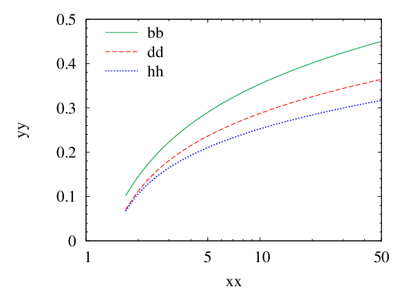
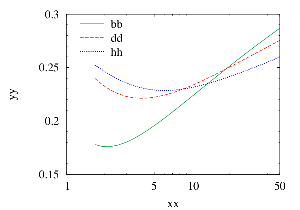
Let us first discuss the power-law behavior (7) of the PDFs, which is not exact and only valid in a certain range of $x$. We fitted power-laws to the CTEQ6L parameterization for $g(x)$, $S(x)$ and $u(x)-d(x)$ in the three intervals $[10^{-5},10^{-4}]$, $[10^{-4},10^{-3}]$ and $[10^{-3},10^{-2}]$. The resulting powers for the gluon and quark singlet distributions are shown in Fig. 1. We see a clear $x$ dependence of the effective power $\lambda$, especially at larger $x$. In Fig. 2 we show the powers obtained in the interval $10^{-4}<x<10^{-3}$ for a larger range of $\mu$. We note that under evolution the powers for the gluon and the quark singlet become similar but remain different up to very high $\mu$. This effect has already been pointed out in [23]. For the non-singlet distribution $u-d$ the effective power $\lambda$ is between $-0.41$ and $-0.42$ in all three $x$ intervals. It changes by less than $1\%$ under evolution in the $\mu$ range corresponding to Figs. 1 and 2.

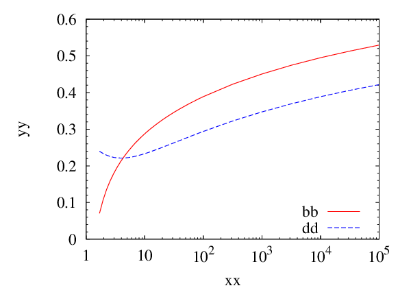
According to (2) there is no simple relation between the ranges of $x$ and $\xi$ in which the same power-law behavior should approximately hold for a PDF and the corresponding GPD. For simplicity we have fitted $H^{g}(\xi,\xi)$, $H^{S}(\xi,\xi)$ and $H^{u-d}(\xi,\xi)$ to power laws (8) in the same $\xi$ intervals that we took for the PDFs. An example of such a fit is shown in Fig. 3, where we see that $H^{g}(\xi,\xi)$ indeed follows an approximate power-law over about one order of magnitude in $\xi$ but not over the full range of the plot. We find that corresponding powers $\lambda$ for PDFs and GPDs differ by at most $3\%$ in the respective $x$ and $\mu$ ranges of Figs. 1 and 2. An exception is the quark singlet distribution in the interval $10^{-3}<x<10^{-2}$, where the power for the GPD is higher than that for the PDF by $5\%$ to $10\%$. This is not surprising, given that already in Fig. 1 we see a more rapid change of the effective power at higher $x$. For definiteness we will evaluate $R_{b}(\lambda)$ and $R_{\text{Sh}}(\lambda)$ with the powers fitted to the PDFs. We have checked that our conclusions do not change when taking the powers for the GPDs instead.

We note that in a specific joint limit of large $\mu$ and $1/\xi$, the solutions of the LO evolution equations for PDFs exhibit so-called double logarithmic scaling [24]. In this case one obtains $\partial\ln(xg)/\partial\ell\sim\ell^{-1/2}$ and $\partial\ln(xS)/\partial\ell-\partial\ln(xg)/\partial\ell\approx-(2\ell)^{-1}$, where $\ell=\ln(x_{0}/x)$ with some constant $x_{0}$. The effective powers in (7) are then larger for the gluon than for the quark singlet distribution and depend logarithmically on $x$. Double logarithmic scaling for GPDs in the region $x\geq\xi$ has been discussed in [10].

We have evaluated the skewness ratios $R(\xi,\mu)$ from the evolved GPDs and PDFs for $\xi=3.2\times 10^{-5}$, $3.2\times 10^{-4}$ and $3.2\times 10^{-3}$. This is compared with $R_{b}(\lambda)$ and $R_{\text{Sh}}(\lambda)$ calculated with $\lambda$ from our fits of the PDFs at the corresponding scale $\mu$ and in the corresponding $x$ interval $[10^{-5},10^{-4}]$, $[10^{-4},10^{-3}]$ and $[10^{-3},10^{-2}]$. The result for gluons is shown in Figs. 6 and 6, where in the initial condition we have taken $b=2$. At the starting scale $\mu_{0}=1.3\operatorname{GeV}$ the curves for $R^{g}(\xi,\mu)$ and $R_{2}^{g}(\lambda)$ coincide as they should, whereas for increasing $\mu$ they become different. This means that one obtains different results for $H^{g}(\xi,\xi;\mu)$ when making the ansatz (2) at scale $\mu$ or when making it at scale $\mu_{0}$ and then evolving the GPD. The difference is however fairly small.

The curves for $R^{g}(\xi,\mu)$ and those for $R^{g}_{\text{Sh}}(\lambda)=R^{g}_{\lambda+1}(\lambda)$ in Figs. 6 and 6 are rather close to each other. At the starting scale they hardly differ at all, which reflects a particularity of the model ansatz (2) for gluons. This is because the ratio $R^{g}_{b}(\lambda)$ in (3) has a very weak $b$ dependence for small $\lambda$: varying $b$ from $1$ to $\infty$ one obtains for instance $R^{g}_{b}(0.1)$ between $1.072$ and $1.088$. With increasing $\lambda$ the $b$ dependence grows only slowly, with $R^{g}_{b}(0.3)$ between $1.231$ and $1.307$ for $b$ between $1$ and $\infty$. This is also seen in the left panel of Fig. 6, where $R^{g}_{b}(\lambda)$ is given for several $b$ values. The solid curve in this figure is for $b=2$ in the initial condition, but the corresponding results for $b=1$ or $b=8$ differ by less than $0.5\%$ in the $\mu$ range of the figure.

Obviously it is hard to see whether $R^{g}(\xi,\mu)$ tends to $R^{g}_{\text{Sh}}(\lambda)$ under evolution if the two functions are already close at the starting scale. To investigate this further we take a variant of (2), namely

	$\displaystyle H^{g}(x,\xi,t)$	$\displaystyle=x\int_{-1}^{1}d\beta\int_{-1+|\beta|}^{1-|\beta|}d\alpha\;\delta(x-\beta-\xi\alpha)\,$
		$\displaystyle\quad\times h_{b}(\beta,\alpha)\,\beta^{-1}H^{g}(\beta,0,t)$		(12)

with $h_{b}(\beta,\alpha)$ as in (4). This corresponds to a double distribution representation for $x^{-1}H^{g}(x,\xi,t)$ instead of $H^{g}(x,\xi,t)$, and one readily verifies that it gives Mellin moments of $H^{g}(x,\xi,t)$ with a polynomial dependence on $\xi$ as required by Lorentz invariance. An analogous representation was first discussed for the quark GPD of the pion [25] and was recently found to be relevant for polarized gluon GPDs [26]. In the case of $H^{g}$ the ansatz (3) has the peculiar property of giving a zero at $x=0$ that is not required by symmetry and quickly disappears under evolution. One may therefore not take this model too seriously, but it serves the purpose of giving a skewness ratio sufficiently different from the one obtained with the more conventional ansatz (2). This is shown in the right panel of Fig. 6, where the dot-dashed curve corresponds to initial conditions (3) for $H^{g}$ and (2) for $H^{S}$, with $b=2$ in both cases. We see that the ratio $R^{g}$ in the two models indeed tends to a common value after evolution. This value it not exactly equal to $R^{g}_{\text{Sh}}(\lambda)$ but differs from it by less than $2\%$. Such a small difference should not be regarded as significant: the form (3) of $R^{g}_{\text{Sh}}(\lambda)$ is obtained in [4, 22] from an integral of $g(x)$ over $x$ from $\xi/2$ to $1$, assuming the power behavior (7) in the entire interval. This is clearly an approximation.

We now turn to the skewness ratio for the quark singlet distribution, which is shown in Fig. 6. In contrast to the gluon case, different values of $b$ in the ansatz (2) lead to significantly different skewness ratios at the starting scale. Evolution to higher $\mu$ brings the curves of $R^{S}(\xi,\mu)$ for different initial conditions closer to each other. As in the case of gluons, they do not exactly approach the curve we calculate for $R^{S}_{\text{Sh}}(\lambda)$, but again this should not be regarded as significant since the power-law (7) with a fixed value of $\lambda$ is only an approximation for a certain $x$ range.

In the left panel of Fig. 6 we also see a clear difference between the evolved ratios $R^{S}(\xi,\mu)$ and the curves for $R^{S}_{b}(\lambda)$ with $\lambda$ taken at the corresponding scale $\mu$. In general there is hence a notable dependence of $H^{S}$ on the scale where the ansatz (2) is made, especially for larger values of $b$. We find the dependence less pronounced for $b=1$, in agreement with what was found in [7] for $\xi=5.26\times 10^{-2}$.

Based on the inversion of Gegenbauer moments, it was argued in [10] that quark distributions $H^{q}(x,\xi)$ should develop a singular derivative $(\partial/\partial x)H^{q}(x,\xi)$ at $x=\xi$ after evolution. To investigate this, we have numerically calculated $(\partial/\partial x)H^{S}(x,\xi)$ from the difference quotient for successive points in $x$, which around $x=\xi$ were spaced in intervals of $9\times 10^{-7}$. In Fig. 7 we plot $H^{S}(x,\xi)$ together with its logarithmic derivative $(\partial/\partial x)\ln H^{S}(x,\xi)$. Taking the derivative of (2) and making the same approximations which lead to (2), one finds that $(\partial/\partial x)H^{S}(x,\xi)$ is singular at $x=\xi$ for $b\leq 1+\lambda$. Indeed, we see in the figure that at the starting scale the derivative has a singularity for $b=1$ but remains finite for $b=2$. Under evolution a singularity develops for $b=2$, whereas for $b=1$ the logarithmic derivative hardly changes. Notice that in the curves for $H^{S}(x,\xi)$ one can barely recognize that the tangent at $x=\xi$ should be vertical: this illustrates the limitations of rendering a weakly singular derivative in a plot. In contrast to the quark case, the ansatz (2) with $b=1$ or $b=2$ gives a finite value of $(\partial/\partial x)H^{g}(x,\xi)$ at $x=\xi$. We have checked numerically that for both initial conditions the derivative remains finite under evolution, in agreement with what one expects from the analytical representation in [10].

To conclude this section, we briefly investigate the quark non-singlet distribution $H^{u-d}$. In Fig. 8 we show the skewness ratio for different values of $b$ in the initial condition. The corresponding curves for $R^{u-d}_{b}(\lambda)$ are not shown: they coincide with those for $R^{u-d}(\xi,\mu)$ at the starting scale and then remain essentially flat since the effective power $\lambda$ hardly changes with $\mu$ in this case. Under evolution to high scales the curves for different $b$ approach each other and the one for $R^{u-d}_{\text{Sh}}(\lambda)$, although much more slowly than for $R^{g}$ or $R^{S}$.

To investigate the change of the $t$ dependence with evolution, we will use the model (2) with $b=2$ for quarks and gluons. We thus need an ansatz for the GPDs at zero skewness $\xi$ but finite $t$, which is described in this section. In all cases we assume an exponential $t$ dependence that is correlated with $x$. For the valence-type combination of GPDs we take the form proposed in Ref. [27]:

	$\displaystyle H_{v}^{q}(x,0,t)$	$\displaystyle=H^{q}(x,0,t)+H^{q}(-x,0,t)$
		$\displaystyle=q_{v}(x)\mskip 1.5mu\exp\bigl[tf_{q}(x)\bigr]$		(13)

with $x>0$, $q_{v}(x)=q(x)-\bar{q}(x)$ and

	$\displaystyle f_{q}(x)$	$\displaystyle=\alpha^{\prime}_{v}(1-x)^{3}\ln\frac{1}{x}$
		$\displaystyle\quad{}+B_{q}(1-x)^{3}+A_{q}\mskip 1.5mux(1-x)^{2}\,.$		(14)

The values $\alpha_{v}^{\prime}=0.9\operatorname{GeV}^{-2}$, $B_{u}=B_{d}=0.59\operatorname{GeV}^{-2}$, $A_{u}=1.22\operatorname{GeV}^{-2}$ and $A_{d}=2.59\operatorname{GeV}^{-2}$ together with the CTEQ6M parameterization for $q_{v}(x)$ at $\mu=2\operatorname{GeV}$ lead to a good description of the data for the Dirac form factors $F_{1}(t)$ of proton and neutron, which are obtained by combining $\int dx\,H_{v}^{q}(x,0,t)$ for $u$ and $d$ quarks with the appropriate charge factors.

For small $x$ we can approximate (4) as $f_{q}(x)\approx\alpha^{\prime}_{v}\ln(1/x)+B_{q}$ and thus have

	$\displaystyle H_{v}^{q}(x,0,t)$	$\displaystyle\approx q_{v}(x)\,x^{-t\alpha^{\prime}_{v}}\,e^{tB_{q}}$
		$\displaystyle\approx a\mskip 1.5mux^{-(1+\lambda+t\alpha^{\prime}_{v})}\,e^{tB_{q}}\,,$		(15)

where in the second step we have assumed a small-$x$ behavior of the valence quark distributions as in (7). Since the $x$ dependence of (4) is a power-law, the integral in (2) can be performed as in Sect. 3, and we can use (3) for the skewness ratio at small $\xi$ after replacing $\lambda$ with $\lambda+t\alpha^{\prime}_{v}$. For $b=2$ this gives

		$\displaystyle H_{v}^{q}(\xi,\xi,t)\approx q_{v}(2\xi)\mskip 1.5mu\exp\bigl[tf_{q}(2\xi)\bigr]\phantom{\frac{1}{1}}$
		$\displaystyle\quad\times\frac{60}{(2-\lambda-t\alpha^{\prime}_{v})(3-\lambda-t\alpha^{\prime}_{v})(4-\lambda-t\alpha^{\prime}_{v})}\,.$		(16)

For small $t$ we can write

	$\displaystyle\frac{1}{n-\lambda-t\alpha^{\prime}}$	$\displaystyle=\frac{1}{n-\lambda}\exp\biggl[-\ln\Bigl(1-\frac{t\alpha^{\prime}}{n-\lambda}\Bigr)\biggr]$
		$\displaystyle\approx\frac{1}{n-\lambda}\exp\biggl[\mskip 1.5mut\mskip 1.5mu\frac{\alpha^{\prime}}{n-\lambda}\mskip 1.5mu\biggr]$		(17)

and thus approximate (4) by

$$H_{v}^{q}(\xi,\xi,t)\approx H_{v}^{q}(\xi,\xi,0)\,\exp\bigl[t\bar{f}_{q}(\xi)\bigr]$$

(18)

with

$$\bar{f}_{q}(\xi)=\alpha^{\prime}_{v}\ln\frac{1}{\xi}+\bar{B}_{q}\,,$$

(19)

where

$$\bar{B}_{q}=B_{q}+\alpha^{\prime}_{v}\,\biggl(\mskip 1.5mu\sum_{n=2}^{4}\frac{1}{n-\lambda}-\ln 2\biggr)\,.$$

(20)

Turning to the gluon distribution, we take

$$H^{g}(x,0,t)=xg(x)\mskip 1.5mu\exp\bigl[tf_{g}(x)\bigr]$$

(21)

with the function

$$f_{g}(x)=\alpha^{\prime}_{g}(1-x)^{2}\ln\frac{1}{x}+B_{g}(1-x)^{2}\,,$$

(22)

which has one parameter less than its counterpart (4). Since most phenomenological information about gluons presently comes from small-$x$ data, it would be difficult to constrain a third parameter. The analog of (4) reads

		$\displaystyle H^{g}(\xi,\xi,t)\approx 2\xi\mskip 1.5mug(2\xi)\mskip 1.5mu\exp\bigl[tf_{g}(2\xi)\bigr]$
		$\displaystyle\quad\times\frac{60}{(3-\lambda-t\alpha^{\prime}_{g})(4-\lambda-t\alpha^{\prime}_{g})(5-\lambda-t\alpha^{\prime}_{g})}$		(23)

for $b=2$ and was already used in [28]. With the approximation in (4) we find

$$H^{g}(\xi,\xi,t)\approx H^{g}(\xi,\xi,0)\,\exp\bigl[t\bar{f}_{g}(\xi)\bigr]\,,$$

(24)

where

$$\bar{f}_{g}(\xi)=\alpha^{\prime}_{g}\ln\frac{1}{\xi}+\bar{B}_{g}$$

(25)

and

$$\bar{B}_{g}=B_{g}+\alpha^{\prime}_{g}\,\Biggl(\mskip 1.5mu\sum_{n=3}^{5}\frac{1}{n-\lambda}-\ln 2\Biggr)$$

(26)

in analogy to the quark case. For our numerical study we take the parameters $\alpha^{\prime}_{\smash[b]{g}}=0.164\operatorname{GeV}^{-2}$ and $B_{g}=1.2\operatorname{GeV}^{-2}$ in order to match recent H1 data on $J\mskip-2.0mu/\mskip-0.5mu\Psi$ photoproduction, whose $t$ dependence is well fitted by

$$\frac{d\sigma}{dt}\propto\exp\biggl[\left(b_{0}+4\alpha^{\prime}_{g}\ln\frac{W_{\gamma p}}{W_{0}}\right)t\,\biggr]$$

(27)

with values $b_{0}=4.63\operatorname{GeV}^{-2}$ and $\alpha^{\prime}_{g}=0.164\operatorname{GeV}^{-2}$ for $W_{0}=90\operatorname{GeV}$ [29]. To connect (27) with (24) we have used the approximate relation $d\sigma/dt\propto|H^{g}(\xi,\xi,t)|^{2}$, which is obtained at tree level when one keeps only the imaginary part of the scattering amplitude. The skewness variable is given by $2\xi=(M_{J\mskip-2.0mu/\mskip-0.5mu\Psi}/W_{\gamma p})^{2}$ in terms of the $\gamma p$ c.m. energy. For simplicity, we have omitted the terms with $1/(n-\lambda)$ in (26) when fixing $B_{g}$. For typical values of $\lambda$ they are quite small.

For antiquarks we set

$\displaystyle H^{q}(-x,0,t)$

$\displaystyle=-\bar{q}(x)\exp\bigl[tf_{\bar{q}}(x)\bigr]$

(28)

with $x>0$. Little is known to date about the $t$ dependence in the sea quark sector. Constraints can be provided by deeply virtual Compton scattering [30, 31], which at small $x$ is sensitive to both sea quark and gluon distributions. A comprehensive analysis of this data, as has recently been performed in [20], is beyond the scope of this work. We will instead explore the pattern of evolution for two extreme choices. In model 1 we set the $t$ slope $f_{\bar{q}}$ equal to the one for valence quarks:

$\displaystyle f_{\bar{u}}$

$\displaystyle=f_{u}\,,$

$\displaystyle f_{\smash{\bar{d}}}$

$\displaystyle=f_{d}\,,$

$\displaystyle f_{\bar{s}}$

$\displaystyle=f_{d}\,,$

(29)

where the choice $f_{\bar{s}}=f_{d}$ has no strong motivation, but does not strongly influence the results we will obtain. In model 2 we set instead

$\displaystyle f_{\bar{q}}$

$\displaystyle=f_{g}$

(30)

for all quark flavors. The initial conditions for evolution of the singlet and non-singlet combinations are then obtained from

	$\displaystyle H^{S}(x,0,t)$	$\displaystyle=\sum_{q=u,d,s}\bigl[H_{v}^{q}(x,0,t)-2H^{q}(-x,0,t)\bigr]\,,$
	$\displaystyle H^{u-d}(x,0,t)$	$\displaystyle=H_{v}^{u}(x,0,t)-H^{u}(-x,0,t)$
		$\displaystyle\quad-H_{v}^{d}(x,0,t)+H^{d}(-x,0,t)\,.$		(31)

For the evolution study in the next section, we make the ansatz (2) with the CTEQ6M parton distributions at $\mu_{0}=2\operatorname{GeV}$, so that we can use the fit of [27] for the $t$ dependence of $H_{v}^{q}(x,0,t)$ as specified at the beginning of this section. In (4) we have neglected the tiny charm quark distribution at $\mu_{0}$. To explore the region of lower scales, we will also consider backward evolution.

In accordance with the analytical considerations in the previous section, we find that at the initial scale the $t$ dependence of $H^{g}(\xi,\xi,t)$ is well described by an exponential form at small $t$ and $\xi$. Evolving to higher scales we still find an approximately exponential behavior in both model 1 and 2, as shown in Fig. 11 for $\xi=3.2\times 10^{-4}$. A slight departure from an exact exponential in the full region $0\leq-t\leq 1\operatorname{GeV}^{2}$ is however visible at $\mu^{2}=50\operatorname{GeV}^{2}$. Evolving to lower scales, we still find an approximate exponential $t$ dependence at $\mu^{2}=3\operatorname{GeV}^{2}$, but for yet lower scales the situation changes. At $\mu^{2}=2\operatorname{GeV}^{2}$ the distribution $H^{g}(\xi,\xi,t)$ turns negative for $-t$ around $0.5\operatorname{GeV}^{2}$ in model 1 and around $0.3\operatorname{GeV}^{2}$ in model 2, whereas at $\mu^{2}=1.69\operatorname{GeV}^{2}$ we have $H^{g}(\xi,\xi,t)<0$ already for $t=0$. This is due to the behavior of the CTEQ6M gluon density at low scales. Since the gluon distribution in this region varies considerably between different global parton fits, we shall not elaborate on this issue further here.

The singlet distribution $H^{S}(\xi,\xi,t)$ is again well approximated by an exponential in $t$ at the starting scale, and it stays exponential to high accuracy in model 2 up to $\mu^{2}=50\operatorname{GeV}^{2}$ and even down to $\mu^{2}=2\operatorname{GeV}^{2}$. As shown in Fig. 11, this is however not the case in model 1. Here we find a clear departure from an exponential behavior even when evolving from the starting scale to $\mu^{2}=6\operatorname{GeV}^{2}$, whereas under backward evolution $H^{S}(\xi,\xi,t)$ rapidly turns negative for some value of $t$. We notice that in model 1 the $x$ dependence of $H^{S}(x,0,t)$ at the starting scale rapidly changes with $t$ due to the large value of $\alpha^{\prime}_{v}$. This induces a corresponding change in the $x$ dependence of $H^{S}(x,\xi,t)$, which enters in the evolution equations.

To quantify the change of the $t$ dependence under evolution, we fit the GPDs at given $\xi$ and $\mu$ to

$$H^{i}(\xi,\xi,t;\mu)=H^{i}(\xi,\xi,0;\mu)\,\exp\bigl[t\bar{f}_{i}(\xi;\mu)\bigr]$$

(32)

for $-t$ between $0$ and $0.5\operatorname{GeV}^{2}$, where $i=g,S$. Given the behavior of the distributions under backward evolution, we restrict these fits to $\mu^{2}\geq 4\operatorname{GeV}^{2}$. Whereas for $H^{S}$ in model 2 and for $H^{g}$ in both models the form (32) gives an excellent description in the kinematical region of the fit, the corresponding fit for $H^{S}$ in model 1 can only be approximate, as is seen in Fig. 11. This must be kept in mind when interpreting the subsequent results, but despite this caveat the corresponding $t$ slope $\bar{f}_{S}$ gives a fair account of how $H^{S}(\xi,\xi,t)$ changes with $\mu$. The results of the fit are shown in Fig. 11 for the starting scale and for $\mu^{2}=50\operatorname{GeV}^{2}$. We see that over a wide region of small $\xi$ the dependence of $\bar{f}_{i}(\xi;\mu)$ on $\xi$ remains logarithmic after evolution to higher scales. For given $\mu$ we can hence perform a fit

$$\bar{f}_{i}(\xi;\mu)=\alpha^{\prime}_{i}(\mu)\ln\frac{1}{\xi}+\bar{B}_{i}(\mu)\,.$$

(33)

The results of such a fit in the range $3.2\times 10^{-5}<\xi<3.2\times 10^{-4}$ are shown in Fig. 11, where we plot $\bar{f}_{i}(\xi;\mu)$ at the midpoint $\xi=10^{-4}$ of the fit range, as well as the effective shrinkage parameter $\alpha^{\prime}_{i}(\mu)$. In model 2, $\bar{f}_{i}(\xi;\mu)$ and $\alpha^{\prime}_{i}(\mu)$ are equal for the gluon and the quark singlet to a good precision at the starting scale by construction. They change rather mildly under evolution to higher scales, but a visible difference between gluon and singlet appears, especially for $\alpha^{\prime}_{i}$. In model 1, we see that the slope and the shrinkage parameter for the singlet evolve quite strongly and tend to approach the corresponding values in the gluon distribution, which increasingly dominates evolution with increasing $\mu$. The respective values for the gluon and the quark singlet are however clearly different even at $\mu^{2}=50\operatorname{GeV}^{2}$.

We have also investigated the evolution behavior of the non-singlet quantity $H^{u-d}(\xi,\xi,t)$. Only the flavor difference enters for the sea quark distributions (28) in this case, and we restrict our investigation to model 1. The $t$ dependence changes in a similar way as for the quark singlet in model 1, as becomes evident from comparison of Fig. 11 and Fig. 12. In particular, evolution to higher scales modifies the exponential behavior of the initial condition. A fit of the $t$ slope for $-t$ between $0$ and $0.5\operatorname{GeV}^{2}$ must hence be taken with the same caveat as above. The $t$ slope $\bar{f}_{u-d}(\xi;\mu)$ fitted as in (32) shows an approximately logarithmic $\xi$ behavior in the full range $2\operatorname{GeV}^{2}\leq\mu^{2}\leq 50\operatorname{GeV}^{2}$, so that we can again perform a fit to the form (33) in the region $3.2\times 10^{-5}<\xi<3.2\times 10^{-4}$. Between $\mu^{2}=2\operatorname{GeV}^{2}$ and $50\operatorname{GeV}^{2}$, the resulting shrinkage parameter $\alpha^{\prime}_{u-d}$ increases only by about 2%, and the slope $\bar{f}_{u-d}(\xi;\mu)$ at $\xi=10^{-4}$ decreases by about 10%. Compared with the quark singlet sector in model 1, evolution effects in the non-singlet sector are hence considerably weaker.

We have studied several aspects of the evolution behavior of GPDs at small $\xi$. To do this, we assumed a particular form of the GPDs at a moderately low scale and numerically evolved this model ansatz to higher $\mu$. At $t=0$ we have taken initial conditions for which $H(\xi,\xi,0)$ and the corresponding parton density $H(\xi,0,0)$ approximately obey power-laws with the same power. Under evolution to higher scales this power changes but remains the same for a GPD and the associated PDF. As a consequence, the skewness ratio $R(\xi,\mu)$ is only weakly $\xi$ dependent, to the extent that the effective power changes with $\xi$. The values of $R(\xi,\mu)$ for different initial conditions approach each other with increasing $\mu$, and at high scales they are well approximated by the Shuvaev formula (3). This convergence is however not very fast: with rather different values of $R(\xi,\mu)$ at $\mu^{2}=m_{c}^{2}$ it only becomes visible at $\mu^{2}$ of a few $10\operatorname{GeV}^{2}$ for the gluon and quark singlet distributions, and at yet larger values in the non-singlet sector. We have not attempted to study how the situation would change for initial conditions at much lower scale, considering that in this case the leading-order approximation of the evolution equations would no longer be suitable for drawing quantitative conclusions. We confirm the finding of [10] that evolution to higher scales generates a singular derivative $(\partial/\partial x)H(x,\xi,t)$ at $x=\xi$ for quarks, but not for gluons.

To study the change of $t$ dependence under evolution, we have chosen initial conditions at $\mu_{0}=2\operatorname{GeV}$ such that $H(\xi,\xi,t)\sim\exp[t\bar{f}(\xi)]$ and $\bar{f}(\xi)=\alpha^{\prime}\ln(1/\xi)+\bar{B}$ at small $\xi$ and $t$. For distributions with a small shrinkage parameter $\alpha^{\prime}$, we find that to a good approximation the $t$ dependence remains exponential under evolution to higher (and to some extent also to lower) scales. In contrast, a deviation from an exponential $t$ behavior becomes visible after evolution rather quickly for distributions with large $\alpha^{\prime}$ at the starting scale, so that a fit to an exponential form is only approximate in these cases. The fitted slopes $\bar{f}(\xi)$ of the evolved GPDs retain a logarithmic $\xi$ dependence, so that one can also determine a shrinkage parameter $\alpha^{\prime}$ at different scales $\mu$. We find that the values of $\alpha^{\prime}$ for the gluon and quark singlet distributions remain close (but not equal) to each other under evolution in a model where they coincide at $\mu_{0}$. In an alternative model, where $\alpha^{\prime}$ for the quark singlet is much larger than for gluons at $\mu_{0}$, evolution brings their values closer to each other, but clear differences remain even at $\mu^{2}=50\operatorname{GeV}^{2}$. An analogous behavior is found for $\bar{f}(\xi)$ at given $\xi$ in both models. We therefore conclude that one may not take it for granted that the $t$ dependence of gluon and sea quark distributions is the same at moderate scales. In the flavor non-singlet sector, we find that $\bar{f}(\xi)$ and $\alpha^{\prime}$ remain quite stable under evolution of the scale.

We thank R. Thorne for drawing our attention to the findings in Ref. [23] and to their explanation within the double logarithmic approximation [24]. This work is supported by the Helmholtz Association, contract number VH-NG-004.

References

- [1] D. Müller, D. Robaschik, B. Geyer, F. M. Dittes and J. Hořejši, Fortschr. Phys. 42 (1994) 101 [hep-ph/9812448].
- [2]
L. Frankfurt, A. Freund, V. Guzey and M. Strikman,
Phys. Lett. B 418 (1998) 345,
Erratum ibid. B 429 (1998) 414
[hep-ph/9703449];
A. Freund and V. Guzey, Phys. Lett. B 462 (1999) 178 [hep-ph/9806267]. - [3] A. D. Martin and M. G. Ryskin, Phys. Rev. D 57 (1998) 6692 [hep-ph/9711371].
- [4] A. G. Shuvaev, K. J. Golec-Biernat, A. D. Martin and M. G. Ryskin, Phys. Rev. D 60 (1999) 014015 [hep-ph/9902410].
- [5] K. J. Golec-Biernat, A. D. Martin and M. G. Ryskin, Phys. Lett. B 456 (1999) 232 [hep-ph/9903327].
- [6] J. Blümlein, B. Geyer and D. Robaschik, Nucl. Phys. B 560 (1999) 283 [hep-ph/9903520].
- [7] I. V. Musatov and A. V. Radyushkin, Phys. Rev. D 61 (2000) 074027 [hep-ph/9905376].
- [8] A. Freund and M. F. McDermott, Phys. Rev. D 65 (2002) 056012, Erratum ibid. D 66 (2002) 079903 [hep-ph/0106115].
- [9] D. Müller and A. Schäfer Nucl. Phys. B 739 (2006) 1 [hep-ph/0509204].
- [10] M. Kirch, A. Manashov and A. Schäfer, Phys. Rev. D 72 (2005) 114006 [hep-ph/0509330].
- [11] I. V. Anikin and O. V. Teryaev, arXiv:0704. 2185 [hep-ph].
- [12] M. Burkardt, Phys. Lett. B 595 (2004) 245 [hep-ph/0401159].
- [13]
M. Göckeler et al. [QCDSF/UKQCD Collaboration],
Eur. Phys. J. A 32 (2007) 445
[hep-lat/0609001];
Ph. Hägler et al. [LHPC Collaboration], arXiv: 0705.4295 [hep-lat]. - [14] A. V. Vinnikov, hep-ph/0604248.
- [15]
D. Müller,
Phys. Lett. B 634 (2006) 227
[hep-ph/0510109];
K. Kumerički, D. Müller, K. Passek-Kumerički and A. Schäfer, Phys. Lett. B 648 (2007) 186 [hep-ph/0605237]. - [16] J. Pumplin, D. R. Stump, J. Huston, H. L. Lai, P. Nadolsky and W. K. Tung, JHEP 0207 (2002) 012 [hep-ph/0201195].
- [17]
M. Diehl,
Phys. Rept. 388 (2003) 41
[hep-ph/0307382];
A. V. Belitsky and A. V. Radyushkin, Phys. Rept. 418 (2005) 1 [hep-ph/0504030]. - [18]
V. Guzey and M. V. Polyakov,
Eur. Phys. J. C 46 (2006) 151
[hep-ph/0507183];
V. Guzey and T. Teckentrup, Phys. Rev. D 74 (2006) 054027 [hep-ph/0607099];
M. V. Polyakov, arXiv:0707.2509 [hep-ph]. - [19]
S. Ahmad, H. Honkanen, S. Liuti and S. K. Taneja,
arXiv:0708.0268 [hep-ph];
S. Ahmad, H. Honkanen, S. Liuti and S. K. Taneja, Phys. Rev. D 75 (2007) 094003 [hep-ph/0611046]. - [20] K. Kumerički, D. Müller and K. Passek-Kumerički, hep-ph/0703179.
- [21] D. S. Hwang and D. Müller, arXiv:0710.1567 [hep-ph].
- [22] J. D. Noritzsch, Phys. Rev. D 62 (2000) 054015 [hep-ph/0004012].
- [23]
A. D. Martin, R. G. Roberts and W. J. Stirling,
Phys. Lett. B 387 (1996) 419
[hep-ph/9606345];
A. D. Martin, R. G. Roberts, W. J. Stirling and R. S. Thorne, Eur. Phys. J. C 4 (1998) 463 [hep-ph/9803445]. - [24]
A. De Rujula, S. L. Glashow, H. D. Politzer, S. B. Treiman,
F. Wilczek and A. Zee,
Phys. Rev. D 10 (1974) 1649;
R. D. Ball and S. Forte, Phys. Lett. B 335 (1994) 77 [hep-ph/9405320]. - [25] A. V. Belitsky, D. Müller, A. Kirchner and A. Schäfer, Phys. Rev. D 64 (2001) 116002 [hep-ph/0011314].
- [26] M. Diehl and D. Yu. Ivanov, arXiv:0707.0351 [hep-ph].
- [27] M. Diehl, T. Feldmann, R. Jakob and P. Kroll, Eur. Phys. J. C 39 (2005) 1 [hep-ph/0408173].
- [28] S. V. Goloskokov and P. Kroll, Eur. Phys. J. C 50 (2007) 829 [hep-ph/0611290].
- [29] A. Aktas et al. [H1 Collaboration], Eur. Phys. J. C 46 (2006) 585 [hep-ex/0510016].
- [30]
F. D. Aaron et al. [H1 Collaboration],
arXiv: 0709.4114 [hep-ex];
A. Aktas et al. [H1 Collaboration], Eur. Phys. J. C 44 (2005) 1 [hep-ex/0505061]. - [31] ZEUS Collaboration, Abstract 68 submitted to EPS07, Manchester, England, 19–25 Jul 2007, ZEUS-prel-07-016.