Hadron interactions from lattice QCD

In Fig. 2, recent theoretical estimates of the $S$-wave $\pi\pi$ scattering lengths, $a_{0}^{0}$ and $a_{0}^{2}$ in units of $1/M_{\pi}$, are summarized [11], where $L$ and $I$ of the scattering length $a_{L}^{I}$ represent the total angular momentum and the total isospin, respectively. The band bounded by two black solid lines represents the theoretically allowed region (universal band)[11]. The three black dots are predictions from 2-flavor chiral perturbation theory (ChPT) at tree, 1-loop and 2-loop levels from left to right. Other results are obtained by using the formulae[12]

	$\displaystyle M_{\pi}(2a_{0}^{0}+7a_{0}^{2})$	$\displaystyle=$	$\displaystyle-6\pi\left(\frac{M_{\pi}}{4\pi F_{\pi}}\right)^{4}\left(\bar{l}_{3}-\frac{193}{210}\right)+M_{\pi}^{4}\alpha_{3}+O(M_{\pi}^{6}),$		(1)
	$\displaystyle M_{\pi}(2a_{0}^{0}-5a_{0}^{2})$	$\displaystyle=$	$\displaystyle\frac{3M_{\pi}^{2}}{4\pi F_{\pi}^{2}}+24\pi\left(\frac{M_{\pi}}{4\pi F_{\pi}}\right)^{4}\left(\bar{l}_{4}-\frac{887}{840}\right)+M_{\pi}^{4}\alpha_{4}+O(M_{\pi}^{6}),$		(2)

where $M_{\pi}^{4}\alpha_{3,4}$ are corrections to ChPT from dispersion integrals. They are approximated at the physical point as

	$\displaystyle M_{\pi}^{4}\alpha_{3}$	$\displaystyle=$	$\displaystyle 0.135+0.77(a_{0}^{0}-0.220)-1.50(a_{0}^{2}+0.0444),$		(3)
	$\displaystyle M_{\pi}^{4}\alpha_{4}$	$\displaystyle=$	$\displaystyle 0.061+0.48(a_{0}^{0}-0.220)-0.26(a_{0}^{2}+0.0444).$		(4)

$\bar{l}_{3,4}$ are the low energy constants in $N_{f}=2$ ChPT and defined by

$\displaystyle M_{\pi}^{2}$

$\displaystyle=$

$\displaystyle M^{2}\{1+\frac{x}{2}\bar{l}_{3}+O(x^{2})\},\quad F_{\pi}=F\{1+x\bar{l}_{4}+O(x^{2})\}$

(5)

with $M^{2}=2Bm$ and $x\equiv M^{2}/(16\pi^{2}F^{2})$. Here $m$ is the quark mass and $F$ is the pion decay constant in the chiral limit. Once $\bar{l}_{3}$ and $\bar{l}_{4}$ are known, the above expressions give $a_{0}^{0}$ and $a_{0}^{2}$.

The red ellipse in the figure corresponds to $\bar{l}_{3}=2.9(2.4)$ from the mass spectrum of the pseudoscalar octet and $\bar{l}_{4}=4.4(2)$ from the scalar form factor of the pion. The narrow azure strip indicates the region allowed if $\bar{l}_{3}$ is treated as free parameter while $\bar{l}_{4}$ is fixed to the above value. There exist several lattice determinations of $\bar{l}_{3}$ and $\bar{l}_{4}$. The MILC collaboration[13], using 2+1 flavors of staggered dynamical quarks, obtain the low energy constants $L_{4,5,6,8}$ of $N_{f}=3$ ChPT, which are translated to $\bar{l}_{3}=0.8(2.3)$ and $\bar{l}_{4}=4.0(6)$ by standard one loop formulae. The results for $a_{0}^{0}$ and $a_{0}^{2}$ are given by a green ellipse in the figure, which is consistent with the previous estimate (the red ellipse). The result of $N_{f}=2$ dynamical Wilson quarks, $\bar{l}_{3}=3.0(5)(1)$[14], with free $\bar{l}_{4}$ leads to the narrow purple strip in the figure, which intersects the red ellipse.

Recent results of the ETM collaboration[15], $\bar{l}_{3}=3.65(12)$ and $\bar{l}_{4}=4.52(6)$, give $M_{\pi}a_{0}^{0}=0.221(1)$ and $M_{\pi}a_{0}^{2}=-0.0427(1)$ (with $M_{\pi}=140$ MeV and $F_{\pi}=93$ MeV), which nicely agree with the red ellipse with smaller errors.

These lattice results for $a_{0}^{0}$ and $a_{0}^{2}$ are indirectly obtained by using $\bar{l}_{3}$ and $\bar{l}_{4}$, which have been determined from the quark mass dependences of $M_{\pi}$ and $F_{\pi}$. There exist several direct estimates on $a_{0}^{2}$ using the finite volume method[1]. The horizontal orange band in Fig. 2 indicates the direct result for $a_{0}^{2}$ by the NPLQCD collaboration[16] with domain-wall valence quarks on a 2+1 staggered sea. Recently they have reported a more accurate result, $M_{\pi}a_{0}^{2}=-0.0443(4)$[17], which is consistent with the red ellipse. So far ChPT predictions and all indirect /direct lattice results agree with each other. However a direct evaluation of $a_{0}^{0}$ is missing. Thus it is a great challenge for lattice QCD to extract $a_{0}^{0}$ directly by the finite volume method.

A less difficult than $a_{0}^{0}$ but still challenging problem is the determination of the $P$-wave scattering phase shift for the $I=1$ two-pion system, from which the $\rho$ meson decay width is extracted. Applying the finite volume method in the laboratory system to this problem, the CP-PACS collaboration has calculated the decay width[18] in lattice QCD with a renormalization group improved gauge action and $N_{f}=2$ dynamical clover quarks on a $12^{3}\times 24$ lattice at $m_{\pi}/m_{\rho}\simeq 0.41$ and the lattice spacing $1/a\simeq 0.92$ GeV. In order to realize the kinematics such that the energy of the two pions is close to $m_{\rho}$, one pion has a non-zero momentum ${\bf p}=(2\pi/L){\bf e}_{3}$ and the other is at rest, while the $\rho$ meson has the same non-zero momentum. Energies of these states for non-interacting hadrons are $W_{1}^{0}=\sqrt{m_{\pi}^{2}+p^{2}}+m_{\pi}$ for the two pions and $W_{2}^{0}=\sqrt{m_{\rho}^{2}+p^{2}}$ for the $\rho$. At $m_{\pi}/m_{\rho}\simeq 0.41$ on a $12^{3}\times 24$ lattice, the invariant mass of two free pions takes the value $\sqrt{s}\simeq 0.97\times m_{\rho}$, which is much closer to $m_{\rho}$ than that in the center of mass system, $E=2\sqrt{m_{\pi}^{2}+p^{2}}\simeq 1.47m_{\rho}$. The hadron interaction shifts the energies from $W_{n}^{0}$ to $W_{n}$, which are related to the two-pion scattering phase shift $\delta$ in the infinite volume through the Rummukainen-Gottlieb formula[19].

To extract two energy levels $W_{n}$ close to each other, a $2\times 2$ matrix of the time correlation function

$$G(t)=\left(\begin{array}[]{cc}\langle 0|(\pi\pi)^{\dagger}(t)(\pi\pi)(t_{s})|0\rangle&\langle 0|(\pi\pi)^{\dagger}(t)\rho_{3}(t_{s})|0\rangle\\ \langle 0|\rho_{3}^{\dagger}(t)(\pi\pi)(t_{s})|0\rangle&\langle 0|\rho_{3}^{\dagger}(t)\rho_{3}(t_{s})|0\rangle\end{array}\right)$$

(6)

has been constructed, where $\rho_{3}(t)$ is an interpolating operator for the neutral $\rho$ meson with the momentum ${\bf p}$ and the polarization vector parallel to ${\bf p}$, and $(\pi\pi)(t)$ is an interpolating operator for two pions, $(\pi\pi)(t)=(\pi^{-}({\bf p},t)\pi^{+}({\bf 0},t)-\pi^{+}({\bf p},t)\pi^{-}({\bf 0},t))/\sqrt{2}$. Two energy levels are obtained from two eigenvalues $\lambda_{n}(t,t_{R})$ of the matrix $M(t,t_{R})=G(t)G^{-1}(t_{R})$ as

$$\lambda_{n}(t,t_{R})=e^{-W_{n}(t-t_{R})}$$

(7)

for large $t$. To keep symmetry between source and sink in $G(t)$ U(1) noises are introduced. The total number of quark propagators per configuration becomes 520, including 10 noises times 2 source points[18].

From the energy levels $W_{n}$ extracted, the invariant mass and the momentum $k$ are given by $\sqrt{s}=\sqrt{W_{n}^{2}-p^{2}}$ and $k^{2}=s/4-m_{\pi}^{2}$, assuming the continuum dispersion relation, while they become $\cosh(\sqrt{s})=\cosh(W_{n})-2\sin^{2}(p/2)$ and $2\sin^{2}(k/2)=\cosh(\sqrt{s}/2)-\cosh(m_{\pi})$, using a lattice dispersion relation. Then $W_{1}$ leads to $\tan\delta=0.0791(9)$ at $\sqrt{s}=0.776(8)$ (continuum dispersion) or $\tan\delta=0.074(7)$ at $\sqrt{s}=0.800(8)$ (lattice dispersion), and $W_{2}$ gives $\tan\delta=-0.38(11)$ at $\sqrt{s}=0.95(3)$ (continuum) or $\tan\delta=-0.52(14)$ at $\sqrt{s}=0.98(3)$ (lattice). In both cases it is observed that $\delta>0$ (attractive) at $\sqrt{s}<m_{\rho}=0.86(1)$ while $\delta<0$ (repulsive) at $\sqrt{s}>m_{\rho}$. This property confirms the existence of a resonance at a mass around $m_{\rho}$[20].

In Fig. 3, $\sin^{2}\delta$, which is proportional to the scattering cross section of the two-pion system, is plotted against the invariant mass $\sqrt{s}$. The two lines in the figure represent fits of the data by

$$\tan\delta=\frac{g_{\rho\pi\pi}}{6\pi}\frac{k^{3}}{\sqrt{s}(M_{R}^{2}-s)},$$

(8)

where $M_{R}$ is the resonance mass, plotted also in the upper panel of Fig. 3, and $g_{\rho\pi\pi}$ is the effective coupling of $\rho\pi\pi$. If $g_{\rho\pi\pi}$ were obtained at several quark masses, it could be extrapolated to the physical quark mass. Since this calculation is performed only at one quark mass, however, it is assumed that $g_{\rho\pi\pi}$ is independent of the quark mass, so that the $\rho$ meson decay width at the physical quark mass is estimated by

$$\Gamma^{\rm ph}=\frac{g_{\rho\pi\pi}^{2}}{6\pi}\frac{(k^{\rm ph})^{3}}{(m_{\rho}^{\rm ph})^{2}}=g_{\rho\pi\pi}^{2}\times 4.128{\rm MeV},$$

(9)

where $(k^{\rm ph})^{2}=(m_{\rho}^{\rm ph})^{2}/4-(m_{\pi}^{\rm ph})^{2}$. The fit result of $g_{\rho\pi\pi}$ gives $\Gamma^{\rm ph}=162(35)$ MeV (continuum) and $\Gamma^{\rm ph}=140(27)$MeV (lattice), which are consistent with the experiment value, $\Gamma=150$ MeV.

Since the first attempt is successful, the next step is the chiral extrapolation. The $\rho$ meson decay width is a good bench mark quantity which shows the dynamical nature of QCD vividly. Therefore collaboration groups which have full QCD configurations at small quark masses are encouraged to calculate this quantity.

In Ref. [21], the energy of two heavy baryons has been measured as a function of the distance $r$ between two heavy quarks $Q$, using quenched QCD with the plaquette gauge action and the Wilson quark action at $a\simeq 0.19$ fm on a $20^{3}\times 24$ lattice. The binding energy of two baryons, $V_{\rm BB}-2V_{\rm B}$, is plotted as a function of $r$ in Fig. 4 at $m_{\pi}\simeq 500$ MeV for the light quark, where $V_{\rm BB}$ is an energy for two baryons while $V_{\rm B}$ is an energy for one baryon. The differences of the three figures are explained in the caption. Surprisingly, the binding energy is very small and shows almost no dependence on $r$ for all three cases. Thus, a repulsive core is not seen for the heavy baryon potential in this calculation.

In Ref. [22], the binding energy of two heavy-light mesons has been computed, each of which is made of one static quark and one light quark, using quenched QCD with the DBW2 gauge action at $a\simeq 0.1$ fm and the Wilson quark action at $m_{\pi}\simeq 400$ MeV. The central potential for total spin $S$ and isospin $I$ of two light quarks in a meson-meson system is decomposed as

$$V_{I,S}(r)=V_{1}(r)+(\sigma_{1}\cdot\sigma_{2})V_{\sigma}(r)+(\tau_{1}\cdot\tau_{2})V_{\tau}(r)+(\sigma_{1}\cdot\sigma_{2})(\tau_{1}\cdot\tau_{2})V_{\sigma\tau}(r)$$

(10)

where $\sigma_{i}$ ($\tau_{i}$) acts on the spin (isospin) of the light quark $q_{i}$, and $r$ is the distance between the two static quarks. Results for $V_{X}(r)$ ($X=1,\sigma,\tau,\sigma\tau$) are plotted in Fig. 5. All potentials show attraction at short distance ($r\leq 0.2$ fm ).

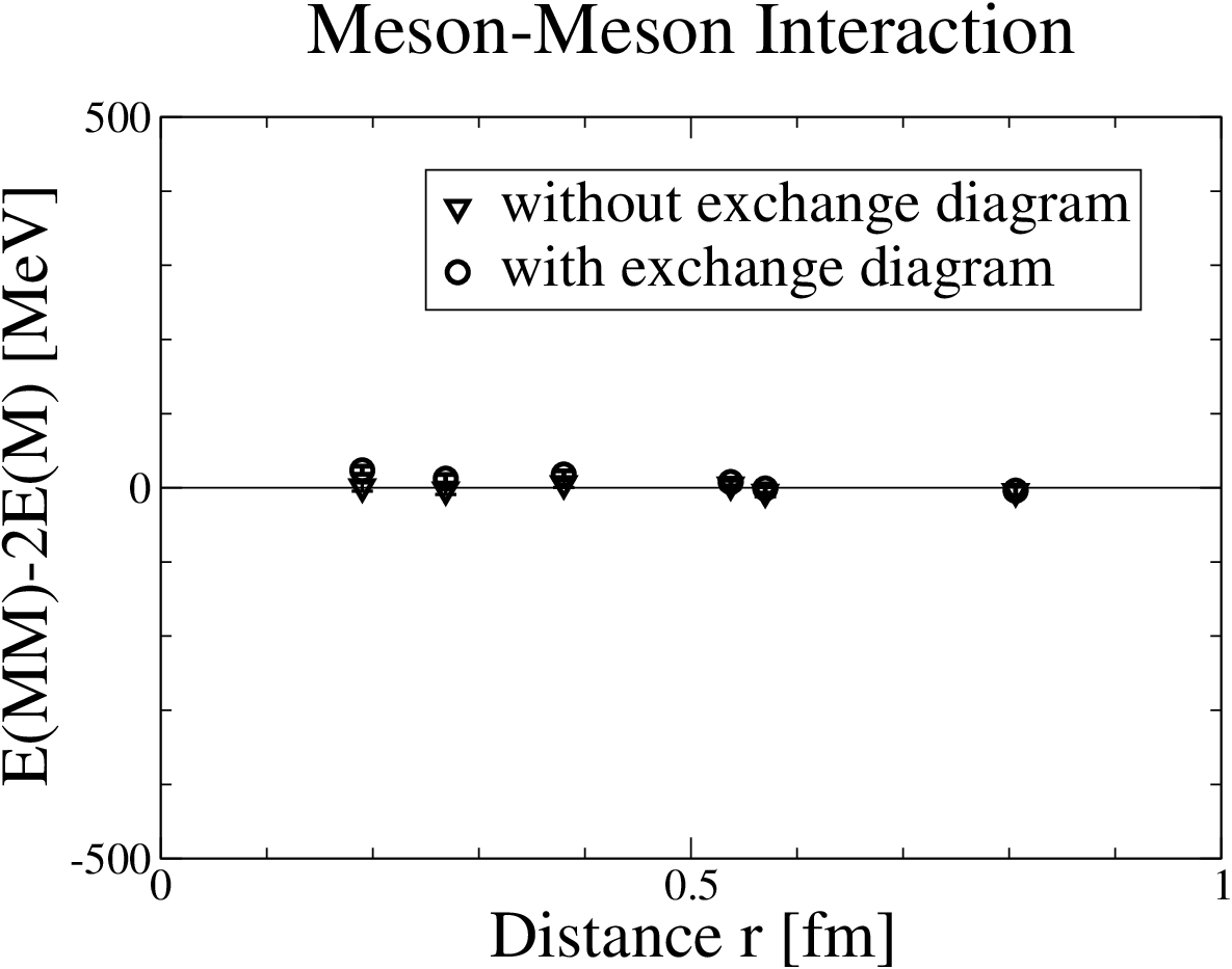
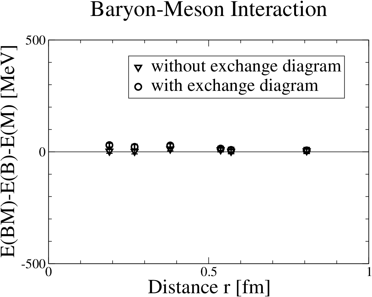
In Ref. [23], a meson-meson potential and a meson-baryon potential has been calculated with the same setup of the baryon-baryon case in the previous subsection. As shown in Fig. 6, however, the dependence on $r$ is very small in both cases. In particular, no short-distance attraction is observed for the two heavy-light mesons, contrary to the results in Fig. 5. There are several candidates which might cause the difference: the light quark mass, the lattice spacing, the lattice volume, the statistics or the way to extract the binding energy. Further investigations are necessary for definite conclusions about the static quark approach to potentials between hadrons.

The starting point of the new method for the $NN$ potential is a wave function defined by

$\displaystyle\varphi({\bf r},E)$

$\displaystyle=$

$\displaystyle\langle 0|N({\bf x},0)N({\bf y},0)|2N;E\rangle,\qquad{\bf r}={\bf x}-{\bf y},$

(11)

where $N({\bf x},t)$ is an interpolating field of the nucleon, $|2N;E\rangle$ is a 2$N$ state with energy $E<E_{\rm inelastic}$ with the inelastic threshold energy $E_{\rm inelastic}$ of the 2$N$ system. This wave function was first analyzed for a spin model in Ref. [25], and has been employed in lattice QCD to calculate the $\pi\pi$ scattering length[26].

This wave function has the following properties. For large enough $r=|{\bf r}|$, $(H_{0}-E)\varphi({\bf r},E)=0$, where $H_{0}=\displaystyle\frac{-\nabla^{2}}{2\mu}$ is a free non-relativistic Hamiltonian with the reduced mass $\mu=m_{N}/2$. This means that the interaction between two nucleons vanishes for a large separation. Moreover, for example in the case of the ${}^{1}S_{0}$ channel, it can be shown that

$\displaystyle\varphi^{S}({\bf r},E)$

$\displaystyle\sim$

$\displaystyle e^{i\delta_{0}(k)}\frac{\sin(kr+\delta_{0}(k))}{kr}+\cdots,$

(12)

where $\delta_{0}(k)$ is the $S$ wave scattering phase shift and $k$ is determined by $E=k^{2}/(2\mu)$. In Ref. [26, 27], it is shown for a two-pion system that

$\displaystyle\varphi^{S}({\bf r},E)$

$\displaystyle=$

$\displaystyle e^{i{\bf kr}}+\frac{ik}{4\pi r}H(k;k)j_{0}(kr)+{\bf P}\int\frac{d^{3}p}{(2\pi)^{3}}\frac{H(p;k)j_{0}(pr)}{p^{2}-k^{2}}+I_{\rm others}({\bf r}),$

(13)

where $H(p,k)=(E_{k}+E_{p})M(p,k)/(8E_{k}E_{p})$ with $E_{p}=\sqrt{m_{\pi}^{2}+p^{2}}$ and $M(p,k)$ is the (off-shell) scattering amplitude. A similar but a little more complicated expression can be shown also for the $NN$ system[28]. For large $r$, if $E<E_{\rm inelastic}$, the contribution from $I_{\rm others}$ vanishes exponentially and eq.(13) approaches eq.(12).

The potential is defined from the wave function through the Schrödinger equation

$\displaystyle[H_{0}+V({\bf r})]\varphi({\bf r},E)$

$\displaystyle=$

$\displaystyle E\varphi({\bf r},E),$

(14)

which symbolically gives

$\displaystyle V({\bf r})$

$\displaystyle=$

$\displaystyle\frac{(E-H_{0})\varphi({\bf r},E)}{\varphi({\bf r},E)}.$

(15)

A corresponding lattice wave function in a finite box at $E\simeq 0$ is given explicitly by

$\displaystyle\varphi({\bf r},E)$

$\displaystyle\equiv$

$\displaystyle\frac{1}{24}\sum_{{\cal R}\in{\cal O}}\frac{1}{L^{3}}\sum_{\bf x}P_{ij}^{I}P_{\alpha\beta}^{S}\langle 0|N_{\alpha}^{i}({\cal R}[{\bf r}]+{\bf x},0)N({\bf x},0)|2N;E\rangle,$

(16)

where $N_{\alpha}^{i}=\varepsilon_{abc}(^{t}q^{a}C\gamma_{5}\tau_{2}q^{b})q_{\alpha}^{i,c}$, $P^{1}=1$ and $P^{0}=\tau_{2}$ are isospin projections, $P^{1}=1$ and $P^{0}=\sigma_{2}$ are spin projections, and the summation over ${\bf x}$ gives zero total momentum. The summation over the discrete rotations ${\cal R}$ of the cubic group ${\cal O}$ implies that the state belongs to the $A_{1}^{+}$ representation of the cubic group, which is expected to couple to an $L=0$ ground state as well as $L\geq 4$ excited states of the rotation group in the continuum theory.

The wave function without projections has been extracted from the 4-point nucleon correlator as

$\displaystyle F_{\rm NN}({\bf x},{\bf y},t;t_{0})$

$\displaystyle\equiv$

$\displaystyle\langle 0|N_{\alpha}^{i}({\bf x},t)N_{\beta}^{j}({\bf y},t){\cal J}_{\rm NN}|0\rangle=\sum_{n}A_{n}\langle 0|N_{\alpha}^{i}({\bf x},t)N_{\beta}^{j}({\bf y},t)|2N;E_{n}\rangle e^{iE_{n}(t-t_{0})}$

(17)

where $A_{n}=\langle 2N;E_{n}|{\cal J}_{\rm NN}(t_{0})|0\rangle$ and ${\cal J}_{\rm NN}(t_{0})=P_{ij}^{I}P_{\alpha\beta}^{S}{\cal N}_{\alpha}^{i}{\cal N}_{\beta}^{j}$. In ${\cal N}$, a wall source is employed by replacing $q({\bf x},t_{0})$ with $Q(t_{0})=\sum_{\bf x}q({\bf x},t_{0})$ after Coulomb gauge fixing. For large enough $t$ the wave function for $E=E_{0}$ is obtained.

In a finite volume, energy levels are shifted from those in the infinite volume as $\Delta E_{n}(L)=E_{n}(L)-E_{n}(L=\infty)=O(L^{-3})$ due to interactions. From these shifts, the scattering phase shift can be extracted[1].

In the actual calculation, the NN scattering for $L=0$ is considered. There are two channels, the spin singlet ($S=0$) channel ${}^{1}S_{0}$ and the spint triplet ($S=1$) channel ${}^{3}S_{1}$, where the standard notation ${}^{2S+1}L_{J}$ is used. Since only a central potential appears for ${}^{1}S_{0}$, the definition (15) directly gives $V_{\rm NN}({\bf r})=V_{\rm C}(r)$. On the other hand, in the case of ${}^{3}S_{1}$, the potential becomes $V_{\rm NN}({\bf r})=V_{\rm C}(r)+V_{\rm T}(r)S_{12}({\bf r})$, where $S_{12}({\bf r})=3({\bf\sigma}_{1}\cdot{\bf r})({\bf\sigma}_{2}\cdot{\bf r})-({\bf\sigma}_{1}\cdot{\bf\sigma}_{2})$ is the tensor operator. The tensor potential induces mixing between ${}^{3}S_{1}$ and ${}^{3}D_{1}$ states, so that the definition (15) gives the so-called effective central potential, which includes the mixing effect from the ${}^{3}D_{1}$ state as a second order perturbation.

Numerical simulations have been made in quenched QCD on a $32^{4}$ lattice with the plaquette gauge action and the Wilson quark action, at $a\simeq 0.137$ fm from the $\rho$ meson mass. The number of configurations is 2000 for $m_{\pi}\simeq 370$ MeV and 527 MeV, and 1000 for $m_{\pi}\simeq$ 732 MeV. A Dirichlet boundary condition (DBC) in time and a periodic B.C. in space are employed, and the wall source with Coulomb gauge fixing is placed at $t_{0}=5$, to avoid an influence of the DBC. Calculations have been performed on a Blue Gene/L at KEK, which has 57.3 TFlops peak performance. It took about 4000 hours of 512 Nodes (a half-rack, 2.87TFlops peak) with 34–48% sustained speed to complete them.

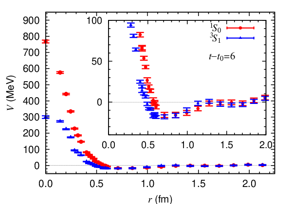
In the left panel of Fig. 7, the $NN$ wave function normalized to 1 at $r\simeq 2.2$ fm is plotted as a function of $r$ for ${}^{1}S_{0}$ and ${}^{3}S_{1}$ at $m_{\pi}\simeq$ 527 MeV. In both cases the wave function shows an increase at 0.5 fm $<r<$ 1.5 fm, suggesting attraction, while it decreases at $r<0.5$ fm, indicating the existence of the repulsive core. In the right panel of Fig. 7 the central (effective central) $NN$ potential extracted from the wave function by eq.(15) at $m_{\pi}\simeq 527$ MeV is plotted as a function of $r$ for ${}^{1}S_{0}$ (${}^{3}S_{1}$). Interestingly the potential obtained qualitatively agrees with the $NN$ potential determined from scattering experiments: weak attraction at long distance, a little stronger attraction at intermediate distance and strong repulsion at short distance (the repulsive core). The solid line is the Yukawa potential (One Pion Exchange Potential) given by

$$V_{\rm C}^{\rm Yukawa}(r)=\frac{g_{\pi N}^{2}}{4\pi}\frac{({\bf\tau}_{1}\cdot{\bf\tau}_{2})({\bf\sigma}_{1}\cdot{\bf\sigma}_{2})}{3}\left(\frac{m_{\pi}}{2m_{N}}\right)^{2}\frac{e^{-m_{\pi}r}}{r},$$

(18)

which agrees well with the data at long distance, with $g^{2}_{\pi N}/(4\pi)\simeq 14.0$ from experiments, $m_{\pi}\simeq 0.527$ GeV and $m_{N}\simeq 1.34$ GeV from lattice data. Thus, in some sense, the Yukawa theory for the nuclear force at $r>1$ fm is confirmed by lattice QCD.

The quark mass dependence of the $NN$ potential for ${}^{1}S_{0}$ is shown in Fig. 8. As the quark mass decreases, the repulsive core at short distance gets stronger, and at the same time, attraction at intermediate distances also becomes a little stronger[29]. In the future it will be interesting to see if this quark mass dependence remains in full QCD.

Since the wave function depends on the energy $E={\bf p}^{2}/(2\mu)$, the potential defined by eq.(15) is also energy dependent in general:

$$V^{J}(r,E)=\frac{(E-H_{0})\varphi^{J}(r,E)}{\varphi^{J}(r,E)},$$

(19)

where $J$, the total angular momentum, is fixed, and $r=|{\bf r}|$. To make our argument simpler, the spin degrees of freedom are not considered here. Since $V^{J}(r,E)$ carries more information than the scattering phase shift $\delta(E)$ does, $V^{J}(r,E)$ is redundant and therefore not physical. For the potential defined from the wave function to be physically meaningful, its energy dependence must be weak for some range of small $E$.

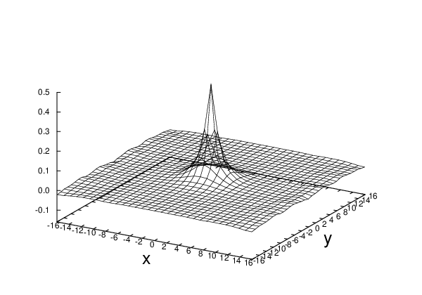
In Fig. 9, the $\pi\pi$ wave function and the corresponding potential in the $S$ channel are shown at ${\bf r}=(x,y,0)$ in quenched QCD at $m_{\pi}/m_{\rho}\simeq 0.51$ for ${\bf p}={\bf 0}$ (left) and ${\bf p}=(2\pi/L,0,0)$ (right) on an $L^{3}$ box[30] . Although the wave functions at the two different energies are very different, the potentials look similar. For the $\pi\pi$ system, the energy dependence of the potential is not so strong at low energy. Note, however, that the wave function (and therefore the potential) at ${\bf p}=(2\pi/L,0,0)$ is calculated at equal time in the laboratory system and is transformed back to the center of mass system, so that the relative time between the two pions is $x$ dependent: $t=v\gamma x$.

In this subsection a method to extract a unique potential from wave functions is proposed[28]. As mentioned in the previous subsection, the potential seems $E$ dependent in general. In addition, it may also depend on the choice of the interpolating operator $N({\bf x},t)$ in (11): one can use a different $\tilde{N}({\bf x},t)$ unless it changes the asymptotic behavior (the phase shift).

To begin with, it is argued that, by introducing a non-local potential, the energy dependence of the potential can be removed. The non-local potential is defined by the following equation,

$\displaystyle K(r,E)$

$\displaystyle\equiv$

$\displaystyle(E-H_{0})\varphi(r,E)=\sum_{r^{\prime}}U(r,r^{\prime})\varphi(r^{\prime},E),$

(20)

where all quantities are taken to be real. For notational simplicity, $\sum$ is used even for the case that a variable is continuous and the superscript $J$ for the angular momentum is omitted here. Since $\{\varphi(r,E)\}_{E}$ form a complete set, there exists an inverse such that

$\displaystyle\sum_{E}\varphi(r,E)\varphi^{-1}(E,r^{\prime})$

$\displaystyle=$

$\displaystyle\delta(r-r^{\prime}),\qquad\varphi^{-1}(E,r)=\sum_{E^{\prime}}\eta^{-1}_{E,E^{\prime}}\varphi(r,E^{\prime})$

(21)

where $\eta^{-1}_{E,E^{\prime}}$ is the inverse of $\eta_{E,E^{\prime}}=\sum_{r}\varphi(r,E)\varphi(r,E^{\prime})$. Using this we obtain

$$U(r,r^{\prime})=\sum_{E}K(r,E)\varphi^{-1}(E,r^{\prime}).$$

(22)

In the actual simulations, it is impossible to obtain $\varphi(r,E)$ for all $E$. If $\varphi(r,E)$’s are obtained for $E=E_{0},E_{1},\cdots,E_{n}$, we expand $U$ in terms of a derivative $d$ such that

$\displaystyle U(r,r^{\prime})$

$\displaystyle=$

$\displaystyle\left[U_{0}(r)+U_{1}(r)d+U_{2}(r)d^{2}+\cdots\right]\delta(r-r^{\prime})=\sum_{k=0}^{n}U_{k}(r)d^{k}\delta(r-r^{\prime}).$

(23)

The coefficient $U_{k}$ can be obtained as

$\displaystyle U_{k}(r)$

$\displaystyle=$

$\displaystyle\sum_{j=0}^{n}K(r,E_{j})\phi_{j,k}^{-1}(r)$

(24)

where $\phi_{j,k}^{-1}$ is the inverse of $\phi_{j,k}=d^{k}\phi(r,E_{j})$. Note that $d$ becomes a difference on a lattice.

It is now argued that the non-local potential $U$ obtained above can be transformed to a local $E$ independent potential $V$. The Schrödinger equations for them become

	$\displaystyle(H_{0}+U)|\varphi,E\rangle$	$\displaystyle=$	$\displaystyle E|\varphi,E\rangle,\quad\langle{r}|U|{r^{\prime}}\rangle=U({r},{r^{\prime}}),\quad\langle{r}|\varphi,E\rangle=\varphi({r},E)$		(25)
	$\displaystyle(H_{0}+V)|\psi,E\rangle$	$\displaystyle=$	$\displaystyle E|\psi,E\rangle,\quad\langle{r}|V|{r^{\prime}}\rangle=V({r})\delta({r}-{r^{\prime}}),\quad\langle{r}|\psi,E\rangle=\psi({r},E),$		(26)

where $H_{0}+U$ is not hermitian unless $U(r,r^{\prime})=U(r^{\prime},r)$, while $H_{0}+V$ is hermitian. Note here that the eigenvalues $E$ in both equations must be equal to ensure that both wave functions give the same scattering phase shift (and the bound state spectrum if any). Existence and uniqueness of $V$ are suggested by the inverse scattering theory, which tells us that a local potential for a fixed $J$ is uniquely reconstructed from the scattering phase shift for all $E$ and informations of possible bound states. Since the eigenfunctions $|\psi,E\rangle$ of the hermitian operator $H_{0}+V$ satisfy $\langle\psi,E|\psi,E^{\prime}\rangle=C_{E}^{2}\delta_{E,E^{\prime}}$, in contrast to $\langle\varphi,E|\varphi,E^{\prime}\rangle=\eta_{E,E^{\prime}}$, the transformation function $\langle{r}|\Lambda|{r^{\prime}}\rangle=\Lambda({r},{r^{\prime}})$ defined by

$\displaystyle|\psi,E\rangle$

$\displaystyle=$

$\displaystyle\Lambda|\varphi,E\rangle,\quad|\varphi,E\rangle=\Lambda^{-1}|\psi,E\rangle,$

(27)

can be constructed as

$\displaystyle\Lambda$

$\displaystyle=$

$\displaystyle\sum_{E,E^{\prime}}|\psi,E\rangle\eta^{-1}_{E,E^{\prime}}\langle\varphi,E^{\prime}|,\qquad\Lambda^{-1}=\sum_{E}|\varphi,E\rangle\frac{1}{C_{E}^{2}}\langle\psi,E|.$

(28)

The compatibility of non-local and local potentials leads to

$\displaystyle\Lambda(H_{0}+U)|\varphi,E\rangle=E\Lambda|\varphi,E\rangle=(H_{0}+V)\Lambda|\varphi,E\rangle,$

(29)

which, together with the completeness of $|\varphi,E\rangle$, implies

$\displaystyle[\Lambda,H_{0}]+\Lambda U$

$\displaystyle=$

$\displaystyle V\Lambda.$

(30)

If the number of degrees of freedom for $E$ and $r$ is denoted as $\#E=\#r=N$ on a finite lattice, eq.(30) gives $N\times N$ constraints, while the unkown $\Lambda$ and $V$ have $N\times N$ and $N$ components, respectively. Therefore the determination of both $\Lambda$ and $V$ from eq.(30) seems an ill-posed problem. However, $N(=\#E)$ components of $\Lambda$ can be taken freely, since the eigenvalue equation (26) does not depend on $C_{E}$, the norm of the eigenfunction, for all $E$’s. Using this freedom, eq.(30) is enough to determine $\Lambda$ and $V$. Eq.(30) is the master equation, which determines the unique local energy independent potential $V$, once a non-local potential $U$ is obtained from a wave function defined through a particular choice of operators. This conceptually solves the uniqueness (or $E$ dependence) problem of ”the potential from a wave function”. The results in the previous section correspond to the 0th order solution of this equation: $V=U_{0}$ and $\Lambda=1$.

To understand interaction properties of hyperons, baryons which include at least one strange quark, is an important subjects in the nuclear physics. Hyperon-nucleon ($YN$) and hyperon-hyperon ($YY$) interactions are relevant to structures of the neutron-star core and the existence/absence of H-dibaryon states. Properties of hypernuclei, nuclei which contain hyperons, will be also studied, as a project at J-PARC (Japan Proton Accelerator Research Complex). However, $YN$ and $YY$ interactions are poorly known both theoretically and experimentally so far. Lattice QCD calculations of the $NN$ potential in the previous section can be extended to $YN$ and $YY$ potentials.

In Fig. 10, the wave function and the corresponding potential for $p\Xi^{0}$ are plotted as a function of $r$ in quenched QCD[31]. The lattice parameters are the same as in the case of the $NN$ potential in the previous section. The light quark mass corresponds to $m_{\pi}\simeq 370$ MeV while the strange quark mass is tuned to reproduce the physical K meson mass, $m_{K}\simeq 550$ MeV. Qualitative features of the $YN$ potential are similar to those of the $NN$ potential. Weak attraction appears at long and intermediate distances while a strong repulsive core shows up at short distance. However the spin dependence of the potential is stronger than in the $NN$ case. In particular, the repulsive core in the ${}^{1}S_{0}$ channel is much stronger than that in the ${}^{3}S_{1}$ channel. Although these results are still preliminary, they are interesting and encouraging as a first step.

Lattice QCD calculations of potentials between hadrons from wave functions have just begun and the first result of the $NN$ potential surprisingly reproduces all the known features of the $NN$ potential such as weak attraction at long distance, a little stronger attraction at intermediate distance and a strong repulsive core at short distance. For a quantitative comparison between lattice results and experimental ones, however, chiral and continuum extrapolations are necessary to remove systematic errors. The inclusion of dynamical quark effects in the $NN$ potential will be the most exciting improvement in future calculations. Now a door is open for us to vast fields in nuclear physics with lattice QCD.

References

- [1] M. Lüscher, Nucl. Phys. B354 (1991) 531.
- [2] H. Yukawa, Proc. Math. Phys. Soc. Japan 17 (1935) 48.
- [3] M. Taketani et al., Prog. Theor. Phys. Suppl. 39 (1967) 1; 42 (1968) 1.
- [4] R. Machleidt and I. Slaus, J. Phys. G27 (2001) R69.
- [5] R. Jastrow, Phys. Rev. 81 (1951) 165.
- [6] H. Heiselberg and V. Pandharipande, Annu. Rev. Nucl. Part. Sci. 50 (2000) 481.
- [7] M. Oka, K. Shimizu and K. Yazaki, Prog. Theor. Phys. Suppl. 137 (2000) 1.
- [8] R. Machleidt, Adv. Nucl. Phys. 19 (1989) 189.
- [9] V.G.J. Stoks, R.A.M. Klomp, C.P.F. Terheggen and J.J. de Swart, Phys. Rev. C49 (1994) 2950.
- [10] R.B. Wiringa, V.G.J. Stoks and R. Schiavilla, Phys. Rev. C51 (1995) 38.
- [11] H. Leutwyler, Contribution to the proceedings of the workshop ”Chiral Dynamics & Experiment”, Durham/Chapel Hill, NC, USA, September 2006 (hep-ph/0612112).
- [12] G. Colangelo, J. Gasser and H. Leutwyler, Nucl. Phys. B603 (2001) 125.
- [13] C. Aubin et al., (MILC Collaboration), Phys. Rev. D70 (2004) 114501.
- [14] L. Del Debio, L. Giusti, M. Lüscher, R. Petronzio and N. Tantalo, JHEP 0702 (2007) 056.
- [15] Ph. Boucaud et al., (ETM Collaboration), hep-lat/0701012.
- [16] S.R. Beane, P.F. Bedaque, K. Orginos and M.J. Savage (NPLQCD Collaboration), Phys. Rev. D73 (2006) 054503.
- [17] S.R. Beane et al., (NPLQCD Collaboration), hep-lat/0706.3026.
- [18] S. Aoki et al., (CP-PACS Collaboration), hep-lat/0708.3705.
- [19] K. Rummukainen and S. Gottlieb, Nucl. Phys. B450 (1995) 397.
- [20] S. Sasaki and T. Yamazaki, Phys. Rev. D74 (2006) 114507.
- [21] T. Takahashi, T. Doi, and H. Suganuma, hep-lat/0601006.
- [22] W. Detmold, K. Orginos and M.J. Savage, hep-lat/0703009.
- [23] T. Takahashi, T. Doi and H. Suganuma, hep-lat/0601008.
- [24] N. Ishii, S. Aoki and T. Hatsuda, Phys. Rev. Lett. 90 (2007) 022001.
- [25] J. Balog et al., Phys. Rev. D60(1999)094508; Nucl. Phys. B618 (2001)315.
- [26] S. Aoki et al., (CP-PACS collaboration), Nucl. Pnys. Suppl. B140 (2005) 479; Phys. Rev. D71 (2005) 094504.
- [27] D. Lin, G. Maryinelli, C.T. Sachrajda and M. Testa, Nucl. Phys. B619 (2001) 467; Nucl. Phys. Suppl. 109A (2002) 218.
- [28] S. Aoki, T. Hatsuda and N. Ishii, in preparation.
- [29] N. Ishii, S. Aoki and T. Hatsuda, PoS (LATTICE 2007) 146.
- [30] K. Sasaki and N. Ishizuka, PoS (LATTICE 2007) 130.
- [31] H. Nemura, N. Ishii, S. Aoki and T. Hatsuda, PoS (LATTICE 2007) 156.